Download Apogee drivers - Linux User Guide V2.1

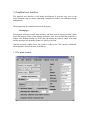
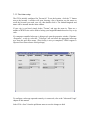
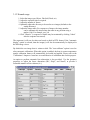
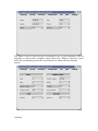
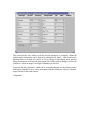
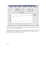
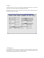
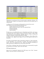
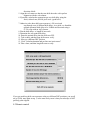
Apogee drivers - Linux User Guide V2.1
Dave Mills ([email protected]) – May 2012
Contents
1. Introduction
2. Installation
3. Graphical User Interface
The Main window
First time setup
Normal usage
Region mode
Focus frame acquisition
Properties window
4. Advanced use
Drift-scan operation
Remote control
5. External packages
Appendix 1 - Processing CCD images
1. Introduction
The Linux Apogee camera drivers have been developed by The Random Factory
(Tucson, AZ) in collaboration with Apogee Inc. The drivers provide both low and high
level interfaces for controlling AP, KX, LISAA and SPH Series cameras. Parallel port,
PCI, and ISA interfaces are supported. This release also includes support for the new
ALTA network and USB models, and Ascent cameras and filter wheels.
2. Installation
The driver and accompanying packages are packaged using the gzipped tar archives. To
install either the runtime, or developer version, log in as the superuser (root), and
• mkdir /opt/apogee
• cd /
• tar xvzf /mnt/cdrom/apogee-driver-x.y.z.tgz
(runtime)
OR
• tar xvzf /mnt/cdrom/apogee-driver-devel-x.y.z.tgz (developer)
where x.y.z is the appropriate version number.
If your cdrom is mounted at a different location (use the "df" command to view the list of
mounted devices), then substitute that path in the command.
This installation will place the files in the directory /opt/apogee. Although it is possible
to install the software to a different location, this is not recommended as it will be
necessary to manually change the location in some of the scripts included with the
drivers.
Run the module installation script
/opt/apogee/modinstall
A couple of pop-up dialogs enquire for the camera type and interface address
(ISA/parallel/PCI/USB interfaces). The installer will check if there is already a precompiled driver module appropriate for your system. If no compatible module is
available the installer will rebuild one from source. If rebuilding is necessary you will
need to install the GCC compiler if it is not already installed.
The appropriate module is loaded and the installer will offer to make the module load
automatically on reboot (the commands to do this are added to the /etc/rc.d/rc.local file).
Once the software is installed, it needs to be configured for each camera user.
Log in as the user, and type
/opt/apogee/install
Once this setup step has been completed, the interface can be started with the command
~/startapogee
3. Graphical user interface.
The graphical user interface is still under development. It provides easy acces to the
major functions such as image acquisition, temperature control, and calibration image
management.
The program may be started from an xterm by typing
~/startapogee
The program will open a small main window, and then create a message window which
shows the progress of the system startup operations. On a slow machine this make take a
minute, on a modern machine (eg 2Ghz cpu), the startup only takes a couple of seconds
and the messages will probably update too quickly to be read.
Once the message window closes, the system is ready for use. The camera is initialized,
and temperature control has been switched on.
3.1 The main window
3.1.1 First time setup
The GUI is initially configured for Tucson,AZ. To set the location, click the "?" button
next to the location. A window will open, showing a list of locations, use the mouse to
scroll the list until you reach your city, then double-click it. The latitude/longitude and
name will be inserted into the main window.
If your city is not listed, simply delete "Tucson" and type the name in. There are a
number of WWW sites can be used to lookup your longitude/latitude based on City or zip
code.
If a computer controlled telescope is being used, open the properties window ("Options>Properties", or Alt-p), select the "Telescope" tab, and select the appropriate telescope
type from the pull down menu. (This facility is not yet completed, LX200 support is
expected for a future release of this package).
To configure a telescope operated remotely via a network, refer to the "Advanced Usage"
chapter of this manual.
Select "File->Save" from the pull-down menu to save the changes to disk.
3.1.2 Normal usage
1. Select the image type (Object, Flat-field, Dark, etc)
2. Adjust the exposure time as required
3. Adjust the number of frames
4. Optionally adjust the directory to be used to save images (defaults to the
startup directory)
5. Adjust the image name. For sequences of images, the image number
can be automatically inserted into the name at any position using a
marker (%d). For example test_%d
6. Click "Observe" (a sequence of frames may be terminated by clicking "Abort"
after the sequence has started).
The exposure(s) will now be taken and saved on disk in FITS format. If the "automatic
display" option is selected, then the image(s) will also be automatically be displayed in
the DS9 image viewer.
By default the raw image data is written to disk. The "auto-calibrate" option is used to
select automatic calibrations. When this option is enabled, the best (ie nearest temperature
match) calibration frames will automatically be loaded and applied. Please refer to the
"Calibrations" chapter to learn how to create libraries of calibration data for this purpose.
An option to perform automatic bias subtraction is also provided. Use the geometry
properties to adjust the frame dimension (BIC, SkipC, and NumY) to provide a
reasonable number of bias columns (6+),
then enter the column numbers in the entry fields provided. Selecting "Automatic bias
subtraction" will then automatically average the data in the bias columns and them from
the image before writing it out. In this case the bias columns will not be included in the
written image.
For the most flexible post-processing, the images are written including IRAF compatible
header information. This allows the images to be easily processed using the IRAF ccdred
package (available as part of the "Linux for Astronomy" cdrom distribution available
from http://www.randomfactory.com/).
In addition to the main window, there are a number of auxillary windows to control less
frequently used facilities. These windows can be accessed via the pull-down menu's, or
via hot-keys.
Alt-p - will open/close the "Properties" window
Alt-c - will open/close the "Calibrations" window
Alt-d - will open/close the "Drift-scan" window
3.1.3 Region mode
To select a sub-region for readout
1. Ensure a full-frame image is displayed in DS9
2. Select "Observe->Region" from the pull-down menu
3. Reply to the pop-up dialog (use current region or define a new one)
4. For new regions, use the mouse to define the region in DS9 using a click-anddrag motion
5. Click the pop-up OK when ready
6. Click "Observe"
Region mode may also be accessed via the "Observe->Continuous" pull-down menu
entry. In this mode, the sub-region will be continuously exposed, readout, and displayed,
until "Abort" is used to stop the sequence. This mode of operation should be useful for
manual focusing. The subregions are not saved to disk when in continuous exposure
mode.
3.1.4 Focus frame acquisition
Focus frames consist of multiple exposures, taken without reading out the image.
Between each exposure, the image is shifted slightly on the detector (either by reading
out a few lines, or by offsetting the telescope slightly), and the focus is also adjusted.
We use the detector shift method, as it also works on manual telescopes.
After each exposure, a pop-up dialog will appear. At this point, manually adjust the focus
by a (hopefully) small known amount, then click OK. After all the exposures are
completed, the frame is read out and written to disk. Special keywords are inserted into
the header to allow the IRAF imfocus task to automatically determine "best" focus (this
feature is still under development).
Support for electronic focus position adjustment will be made available in future releases
of the package.
For systems where no electronic readback of focus position is available it can be
simulated by attatching a calibrated disk to the focusser.
3.2 Properties window
The properties window can be accessed either by selecting "Options->Properties" from
the pull-down menu, or by typing Alt-p whilst the pointer is in the main window. In each
case repeating the operation will close the window again.
The window consists of a set of tabbed panels, click the tab name to view the panel.
Telescope panel
This panel is used to select the type of telescope in use. If your telescope is not yet
supported, or does not have computer control, then select "Manual". Enter the correct
focal ratio, remembering to take into account any focal reducers that are installed.
System
Geometry
This panel provides easy editing of all the relevant parameters to competely define the
readout region. Subregions can be defined by editing StartX, StartY, NumX and NumY.
Binning can be set in each axis, and so on. Every change is immediately tested, and any
illegal combinations will cause the background color of the panel to change. It will not be
possible to obtain an image if an illegal combination is selected.
In general the only parameters which will be manually adjusted are the binning factors.
Sub-region definition is more easily performed using the pull-down "Observe->Region"
menu selection in the main window.
Temperature
This panel provides control and feedback. Select the required target temperature using the
arrows, or type in a new target temperature.
The graph illustrates the last minute or so of temperature readings from the camera. It
often takes about 20 seconds after a new target temperature is requested before the
temperature changes significantly, so be patient.
CCD
This panel shows the ccd sensor details. These are read-only.
Filter
This panel shows available filters and the current selection. (NOT YET
IMPLEMENTED)
Catalogs
This panel is used to define the locations (disk, network) of the most commonly used
catalog resources. The GSC, USNO, RNGC catalogs, and the Digital Sky Survey can be
configured.
Available catalogs can be used to overlay object information (name, mag, etc) on either
your images, or reference images from the Digital Sky Survey.
Catalog data can also be used to automatically calculate the World-Coordinate-System (ie
RA, DEC) parameters for images.
3.3Calibrations
The calibrations window can be accessed either by selecting "Calibrations->[type]" from
the pull-down menu, or by typing Alt-c whilst the pointer is in the main window. In each
case repeating the operation will close the window again.
Obtaining the best performance from ccd cameras requires considerable calibration. This
window provides a simple way to automate the collection of the most common types of
calibration data.
A calibration run will often require careful preparation to ensure the best results.
Each calibration run is specified using the following items
- location of directory used to store the data
- number of frames to average to create each calibration frame
- minimum temperature
- maximum temperature
- exposure duration
The directory to store calibration data may be independently specified for each category
of calibration frame. Each category also has an associated "automatic" option, which,
when selected will activate automatic calibration using that category (assuming that
"automatic calibration" is enabled in the main GUI window.
Clicking one of the "Start [type] calibration" buttons will pop-up a dialog which provides
an estimate of the length of time required to run the full sequence (which can be
substantial).
The software steps through the range of temperatures selected (in 1 degree increments).
At each temperature, a set of [n] frames is acquired. These frames are buffered in
memory. Once all [n] exposures have been acquired, the appropriate calculations are
made to generate the calibration frame, which is then written to disk.
Once a library of calibration frames has been obtained, they can automatically be applied
by selecting the "auto-calibrate" option in the main window.
DS9 Image display tool
Images may be automatically displayed in the DS9 image viewer. Select "automatic
display" in the main window to activate this option.
The DS9 image viewer is a powerful tool. There is extensive online documentation
available at
file:/opt/apogee/html/ds9/index.html
Most aspects are fairly intuitive, configuration is done using the pull-down menus;
contrast/brightness is adjusted by holding down the left-mouse-button, and moving the
mouse around. The middle mouse button centers the image at the current location.
4. Advanced use.
4.1 Drift-scan operation
The driver is equipped with preliminary support for drift-scan operation. In this mode, the
telescope is set at a fixed position, and the sky allowed to drift through the field at the
sidereal rate. The driver automatically reads out the ccd at the appropriate rate to correct
for the sidereal motion.
It is of course crucial that the rate be very accurately specified, and that the readout
software does not get pre-empted by other processes in the system. It is recommended
that during a drift-scan readout, no other major activity is taking place on the computer.
In drift-scan mode, the length of the exposure is limited only by available memory. For
example if sufficient memory where available you could make a single drift-scan from
dusk until dawn. Of course, all the image data will be sitting in the memory of your
computer until the exposure completes, when the data is written to disk. Given the
possibility of a power failure or other computer problem, you should limit your drift-scan
exposures to an hour or so, thus minimising data loss should the unthinkable occur.
Using drift-scan mode will require some setup effort on the part of the user.
Here is a checklist of steps we used to test this mode
1. Ensure that the telescope is VERY well polar aligned
2. Switch off the telescope drive
3. Point the telescope at the celestial equator (DEC=00:00:00)
4. Use short normal mode exposures (~1 minute) to observe the
direction of drift
5. Align the ccd camera so that the stars drift down the ccd in perfect
alignment with the ccd columns
6. If possible, calculate the appropriate per-row drift delay using the
fratio, sidereal rate, and ccd pixel scale (good luck!)
7. Otherwise, take short drift-scan exposures (~500 rows) and
step through a set of different drift delays. As a guide, we found the
optimal equatorial drift delay to be 344000 microseconds using a
8" F/6 scope with an Ap7p camera.
8. Plot the drift-delays vs length-of-star-trails
9. Determine the zero point drift-delay
10. Enter the optimal delay into the drift-scan GUI.
11. Take a short, and then long drift-scan to verify.
12. Move to a different DEC position
13. Click "Calculate duration and per-line rate in microsecs"
14.Take a short, and then long drift-scan to verify.
If you get good long drift scan exposures at the two different DEC positions, you are all
set up. If not, start again at step 1, as the most likely cause is that your telescope is NOT
perfectly polar aligned.
4.2 Remote control
There are three methods for using the software via a remote computer.
1. Standard X-windows
Use the standard X-windows display redirection facility to point
the display to another computer (named "other" for example).
eg. setenv DISPLAY other:0
The "xhost +ccd-name" command must also be issued on the "other"
computer, to allow remote displays to take place (where ccd-name is the
name of the camera control computer).
Finally , start the GUI as usual, the windows should appear on the
"other" machine.
This method only works if both computer are running a *nix type operating
system. X-windows is available for MS Windows, but it is usually expensive.
2. VNC
Use the VNC (Virtual network computing) software (which is free, and open-source).
This package supports the remote viewing on the ccd GUI desktop on *nix, windows,
and Mac platforms. Even better, multiple remote users can simultaneously view the same
dekstop, and even share interaction rights with the applications. Given fast network
connections (fast ethernet) this is a near optimal solution. The VNC package is just one of
the items in the bundle of extras included in the cdrom version of the Linux Apogee
Drivers cd, available from The Random Factory.
Future releases of the driver will also include support for true client/server use of
cameras. In this situation, the GUI will actually run on the remote machine, and only the
low level camera access code will run on the camera controller computer.
3. Client/Server
An experimental client/server mode of operation is also available.
The script /opt/apogee/scripts/startserver will lauch a camera server process which listens
on port 2001 for connections. Commands can be sent from any other computer by
copying the script /opt/apogee/scripts/apogeeclient to the remote machine and editing it to
reflect
the location of the machine hosting the camera. The client machine must have tcl
installed (in /usr/bin/tclsh).
The socket interface is very simple and could easily be driven by user programs written in
any standard programming language.
5. External packages
The Linux Apogee camera driver is free, open source software. However, we do offer an
enhanced distribution on cdrom, which adds a wealth of extra tools for both user and
developer. We can also undertake custom programming projects to enhance the driver
and interface for special requirements. Contact us for a quote.
The following list describes the current contents of the cd distribution
SWIGManual.pdf
- User manual for the Simple Wrapper and Interface Generator package
apogee_devel.tar.gz
- Developers version of the drivers
apogee_runtime.tar.gz
- Standard runtime, user distribution
astrotcl-1.4.4.src.tar.gz - A set of astronomical tools for tcl
ccdlinux-modaudine.tar.gz - The drivers for for the Audine/Gemini open-hardware cameras
cfitsio-2.0.3-4.i386.rpm - C language FITS utilities
ds9.2.0.tar.gz
- The DS9 sources
ds9.linux.2.0.tar.gz
- DS9 for Linux
fiasco-1.0.tar.gz
- Image compression package
fitsTcl-2-0.i386.rpm
- FITS tools for tcl
ftools-2-4.i386.rpm
- Massive astronomical data reduction suite in C/tcl
gimp-1.2.0.tar.gz
- Image manipulation package with extensive capabilities
gimp-data-extras-1.2.0.tar.gz - Add-ons for GIMP
gsl-0.4-1.i386.rpm
- GNU scientific subroutines
imlib-1.9.7-3.i386.rpm
- Image management/conversion library
imlib-cfgeditor-1.9.7-3.i386.rpm - extras for imlib
imlib-devel-1.9.7-3.i386.rpm - devlopers version of imlib
libjpeg-6b-10.i386.rpm - jpeg library
libjpeg-devel-6b-10.i386.rpm - developers version of jpeg library
libpng-1.0.5-3.i386.rpm - PNG library
libpng-devel-1.0.5-3.i386.rpm - developers version of PNG library
libtiff-3.5.4-5.i386.rpm - TIFF library
libtiff-devel-3.5.4-5.i386.rpm - developers version of TIFF library
netpbm.tar.gz
- large set of image conversion utilities
novas-c-2-0.i386.rpm
- Astrometry routines from the US Naval Observatory
opt
- Full unpacked developers version of drivers for easy browsing
python-1.5.2-13.i386.rpm - The python scripting language
python-devel-1.5.2-13.i386.rpm - developers version of python
python-docs-1.5.2-13.i386.rpm - extensive documentation for python
python-tools-1.5.2-13.i386.rpm - extra tools for python
pythonlib-1.23-1.noarch.rpm - python libraries
sexarticle.ps.gz
- description of sextractor
sextractor-2.1-0.i386.rpm - automatic star/galaxy location
skycat-2.5-3.i386.rpm
- feature rich image viewer/catalog access
swig1.3a5.tar.gz
- Simple wrapper and interface generator
vnc-3.3.2r3_unixsrc.tgz
- virtual network computing unix source
vnc-3.3.3beta2_ppc_mac.sit - virtual network computing for mac
vnc-3.3.3r2_x86_linux_2.0.tgz - virtual network computing for linux
vnc-3.3.3r7_x86_win32.zip - virtual network computing for windows
xite-3-4.i386.rpm
- Image processing tools
The Random Factory also produces a very extensive collection of Astronomical software
all pre-compiled for Linux. The current release (Volumes 10) includes over 5GB of
software on a 5-cdrom set.
Appendix 1 - Processing CCD images
This advice is paraphrased from the advice provided to professional Astronomers
observing at the US National Observatory. It is based on a document included with the
IRAF system, and was written by Dr. Phil Massey (currently at Lowell Observatory).
What Calibration Frames Do You Need?
The answer to this depends to some extent on what it is that you are doing. The goal is to
not let the quality of the calibration data degrade your signal-to-noise in any way. If you
are in the regime where the read-noise of the chip is the dominant source of noise on your
program objects, then subtracting a single "bias frame" from your data would increase
the noise prohibitively.
However, if you instead use the average of 25 bias frames, the noise will be increased by
only 10%. Of course, if you are into high signal-to-noise spectroscopy, so you have lots
and lots of signal compared to read-noise, or if you have high sky background on direct
images, so that read-noise is again immaterial, then the signal-to-noise will be little
affected by whether you have only a few bias frames. However, in this regime the quality
of your flat fielding is all important if you want to get the most out of your data.
The following list contains the type of calibration images you may need, and provides
some guide to the consideration of how many you may want to have.
bias frames.
These are zero second integration exposures obtained with the same pre-flash (if any) you
are using on your objects. If read-noise will sometimes dominate your source of error on
the objects, take 25 bias frames per night. Take them over dinner and you'll never notice
it. You will want to have a new sequence of these each day.
dark frames.
These are long exposures taken with the shutter closed. If your longest exposure time is
over 15 minutes you may want to take an equal length dark frame, subtract a bias frame
from it, and decide if you are worried about how much dark current is left. Applications
where dark current will matter are long-slit spectroscopy and surface brightness studies -cases where the background is not removed locally. If you do find that you need to take
care of dark current, then you should take at least 3 and preferably 5 to 10 dark frames
during your run, each with an integration time equal to your longest exposure. You
should ensure that your system is sufficiently light-tight to permit these to be done
during the day.
flat field exposures.
At a minimum, flat field exposures are used to remove pixel-to-pixel variations across
the chip. Usually dome flats (exposures of an illuminated white board) will suffice to
remove the pixel-to-pixel stuff. You will want to expose the dome or projector flats so
that you get sufficient counts to not degrade the signal-to-noise of the final images. If
you are after 1% photometry per pixel then you will need to have several times more
than 10,000 electrons accumulated in your flats, but you need to be careful not to exceed
the good linearity limit in any single flat exposure. Generally if you have 5 or more flats
each with 10,000 electrons per pixel you are probably fine. You will need a set like this
for every filter, and you probably will want to do a new sequence every day.
twilight flats.
If you are interested in good photometry of objects across your field, you need to know if
the sky looks different to your CCD than the dome flat. It is not unusual to find 5-10%
gradients in the illumination response between a flat and a sky exposure, and this
difference will translate directly into a 5-10% error in your photometry. For most
applications, exposures of bright twilight sky (either for direct imaging or spectroscopy)
will cure this problem. With direct imaging this requires you to be very quick on your
feet to obtain a good level of sky exposure in each of your filters while the sky is getting
darker and darker. (Only the truly desperate would take twilight flats in the morning!)
For direct imaging I would recommend 3 to 5 exposures in each filter, stepping the
telescope slightly in between the exposures so that any faint stars can be effectively
cleaned out. You will find that you need to keep increasing the exposure time to maintain
an illumination level of 10,000 electrons.
blank dark sky exposures.
Some observers doing sky-limited direct imaging may wish to
try
exposures of blank sky fields rather than twilight sky, as the color of twilight and the
color the dark sky do differ considerably. Obtain at least three, and preferably four, long
exposures through each filter of some region relatively free from stars , stepping the
telescope 10-15 arcseconds between each exposure. The trick here, of course, is to get
enough counts in the sky exposures to make this worth your while. Unless you are willing
to devote a great deal of telescope time to this, you will have to smooth these blank dark
sky exposures to reduce noise, but the assumption in such a smoothing process is that the
color response of the chip does not vary over the area you are smoothing. You might try
dividing a U dome flat by a V dome flat and seeing how reasonable an assumption this
might be. Also, if the cosmetics are very bad the smoothing process will wreak havoc
with your data if you are not successful in cleaning out bad columns and pixels.
This section will briefly outline what we will do with the calibration images.
Most of the calibration data is intended to remove "additive" effects: the electronic
pedestal level (measured from the overscan region on each of your frames), the pre-flash
level (measured from your bias frames), and, if necessary, the dark current. The flat field
data (dome and twilight sky exposures) will remove the multiplicative gain and
illumination variations across the chip.
When you obtained your frames at the telescope, the output signal was "biased" by
adding a pedestal level of several hundred ADU's. We need to determine this bias level
for each frame individually, as it is not stabilized, and will vary slightly (ss 5-30 ADU's)
with telescope position, temperature, and who knows what else. Furthermore, the bias
level is usually a slight function of position on the chip, varying primarily along
columns. We can remove this bias level to first-order by using the data in the overscan
region, the (typically) 32 columns at the right edge of your frames.
data
We will average the data over all the columns in the overscan region, and fit these values
as a function of line-number (i.e., average in the "x" direction within the overscan region,
and fit these as a function of "y"). This fit will be subtracted from each column in your
frame; this "fit" may be a simple constant. At this point we will chop off the overscan
region, and keep only the part of the image containing useful data. This latter step usually
trims off not only the overscan region but the first and last few rows and columns of your
data.
If you pre-flashed the chip with light before each exposure, there will still be a non-zero
amount of counts that have been superimposed on each image. This extra signal is also
an additive amount, and needs to be subtracted from your data. In addition, there may be
column-to-column variation in the structure of the bias level, and this would not have
been removed by the above procedure. To remove both the pre-flash (if any) and the
residual variation in the bias level (if any) we will make use of frames that you have
obtained with a zero integration time. These are referred to in IRAF as "zero frames"
may also be called "bias frames". We need to average many of these (taken with preflash if you were using pre-flash on your object frames), process the average as described
above, and subtract this frame from all the other frames.
"Dark current" is also additive. On some CCD's there is a non-negligible amount of
background added during long exposures. If necessary, you can remove the dark current
to first-order by taking " dark" exposures (long integrations with the shutter closed),
process- ing these frames as above, and then scaling to the exposure time of your
program frames. However, it's been my experience that the dark current seldom scales
linearly, so you need to be careful. Furthermore, you will need at least 3 dark frames in
order to remove radiation events ("cosmic rays"), and unless you have a vast number of
dark exposures to average you may decrease your signal-to-noise;
The bottom line of all this is that unless you really need to remove the dark current, don't
bother.
The next step in removing the instrumental signature is to flat-field your data. This will
remove the pixel-to-pixel gain variations, and (in the case direct imaging) the largerscale spatial variations. If you are doing direct imaging, then you are probably happy by
normalizing the flat-field exposures to some average value.
The final step in the flat-fielding process is to see if your twilight sky exposures have
been well flattened by this procedure--if not, we may have to correct for this.
Apogee drivers - Programmers Guide V2.1
Dave Mills([email protected]) – May 2012
Contents
1. CameraIO object (ISA/PCI/Parallel port)
2. Alta and Ascent object (USB/NET)
3. Tcl Scripting interface
4. Code generation
5. Tcl/Tk and loadable libraries
6. Ccd library
7. LX library
8. Remote control
1. CameraIO object (ISA/PCI/Parallel port)
In the unlikely event that you should find it necessary to use the C++ interface directly,
there is a small sample of code in the file
/opt/apogee/src/apogee/test_apogee.cpp.
This code should be easily comprehensible to anyone familiar with C++. For example to
create a new camera object
cam = new CCameraIO;
To call a method, for example InitDriver
result = cam->InitDriver(cameraNumber);
To set the value of an instance variable
cam->BaseAddress = 0x378;
2. Alta and Ascent objects (USB/NET)
In the unlikely event that you should find it necessary to use the C++ interface directly,
there is a small sample of code in the directories
/opt/apogee/apps/CPP
/opt/apogee/libapogee/examples
This code should be easily comprehensible to anyone familiar with C++. For example to
create a new camera object
Alta cam;
To call a method, for example InitDriver
result = cam.StartExposure(exptime,shutter);
The full libapogee API is documented in /opt/apogee/doc/libapogee-API
3. Tcl Scripting interface
The simplest way to program using the driver is via the provided scripting interface
libraries. An interface is provided for the Tcl/Tk language. This language is easy to learn
due to its interpretive nature. That is, you type commands directly to a command line, and
they are executed immediately.
Interfaces to other languages (python, perl, and more) can also be automatically generated
using the SWIG package (included in the "devel" release of the package).
To begin a Tcl/Tk session, open an X-terminal, start a csh shell and prepare the
environment by typing
source /opt/apogee/scripts/setup.env
(prepares the environment)
This will initalize your shell to use the included version of "wish" , the Tcl/Tk windowing
shell. Another version of "wish" may already be installed on the system, but it is
recommended that the included version be used to avoid and potential library version
conflicts.
/opt/bin/wish
(starts the tcl/tk shell)
A small gray window will open. Re-select your xterm window and type
source /opt/apogee/scripts/camera_init.tcl
(command line only)
or
source /opt/apogee/scripts/gui.tcl
(gui interface plus command line)
The appropriate driver library will be dynamically loaded, and new commands will be
added to the Tcl shell. Type a "?" at the prompt to get a list of all the commands Tcl is
currently aware of.
The camera_init script also creates a CAMERA variable which acts as a software pointer
to the C++ structure used to control the camera.
Tcl commands typically protect the user against incorrect usage. For example the
CAMERA object may be commanded using the syntax
$CAMERA command [arg1] [arg2] ...
Typing
$CAMERA xyzzy
will result in an error report (because "xyzzy" is not a valid camera command!). This
error report helpfully includes a list of all the commands that the $CAMERA referenced
object does understand.
The most useful commands are listed below.
$CAMERA InitDriver cameraNumber
or
$CAMERA InitDriver cameraNumber 0 0
(ALTA models)
This command needs no additional arguments, it performs camera initialization. It will
not normally be necessary to use this call, as it will have been done as part of the
camera_init.tcl script.
$CAMERA read_Status
This command returns an integer representing the readout status of the camera. Typically
this will be stored in a tcl variable, and then printed out in user friendly format. E.g.
(this example is for ISA/PCI/PPort cameras, the ALTA status codes are slightly different)
set s [$CAMERA read_Status]
switch $s {
0 {set t "Idle"}
1 {set t "waiting for trigger"}
2 {set t "exposing"}
3 {set t "downloading"}
4 {set t "line ready"}
5 {set t "image ready"}
6 {set t "flushing BIR"}
default {set t "ERROR code $s"}
}
puts stdout "Camera status is $s"
$CAMERA Expose duration shutter
or
$CAMERA StartExposure duration shutter (Alta/Ascent)
Take an exposure of the requested duration (expressed in seconds). The value of the
shutter argument is either 0 - leave shutter closed, or 1 - open shutter during exposure.
$CAMERA BufferImage testname
This command retrieves the image from the camera, and saves it in the PC's
memory/swap-space. Any number of images can be buffered in this way, subject to
available memory.
Once the image is in memory it can be manipulated using the commands from the Ccd
library. For example
list_buffers
shows current buffers, their dimensions, bit-depths etc.
write_buffer testname mytest.fits
stores the contents of the buffer "testname" on disk as a FITS format file.
In addition to the "methods" associated with a CAMERA object, there is also a
mechanism for access to the "instance" variables of the CAMERA object. Each instance
variable corresponds to a camera configuration parameter. The syntax for examining the
current value of a parameter is
$CAMERA configure -m_[parameter-name]
and to set the parameter to a new value
$CAMERA configure -m_[parameter-name] new-value
The following instance variables are supported
For ISA/PCI/PPort cameras
BIC BIR BaseAddress BinX BinY Columns CoolerMode CoolerSetPoint CoolerStatus FilterPosition FilterStepPos GuiderRelays HFlush -
Before image columns
Before image rows
Base address of interface
Binning factor for columns
Binning factor for rows
Number of columns on detector
Cooling mode
Target temperature
Status of cooler
Filter position index
Guider relay on/off
Binning factor for column flush
ImgColumns ImgRows Interface LongCable Mode NumX NumY RegisterOffset Rows Shutter SkipC SkipR StartX StartY Status TDI TempScale Temperature Test2Bits TestBits Timeout UseTrigger VFlush -
Imaging columns on detector
Imaging rows on detector
Type of interface
Long cable indicator
Mode
Number of columns to read out
Number of rows to read out
Register offset for multiple cameras
Number of rows
Status of shutter
Number of skip columns
Number of skip rows
First column to read out
First row to read out
Camera readout status
Drift mode
Scale multiplier for raw temperature
Current ccd temperature
Second set of test bits
Primary set of test bits
Image readout timeout
Trigger status
Binning factor for vertical flush
For ALTA cameras
CameraId Camera number
CameraInterface 0=NET, 1=USB
CameraModel Model code
ClampColumns Clamp columns
Color 1 if color ccd
DataBits 0=16 bits, 1=12 bits
DefaultGainTwelveBit – gain 0 to 1024
DefaultOffsetTwelveBit - offset
DefaultRVoltage Voltage
DigitizeOverscan - 1 = digitize overscan region
HFlushDisable 1 = Disable horizontal flushing
ImagingColumns - Number of imaging columns
ImagingRows Number of imaging rows
InterlineCCD 1 = interline ccd
MinSuggestedExpTime – minimum recommended exposure
OverscanColumns - Number of overscan columns
OverscanRows Number of overscan rows
PixelSizeX Pixel x size in microns
PixelSizeY Pixel y size in microns
PostRoiSkipColumns – Post ROI skip
PreRoiSkipColumns – Pre ROI skip
ReportedGainSixteenBit ResetVerticalArrays – 1 = Reset vertical arrays
RoiBinningH Horizontal binning
RoiBinningV Vertical binning
RoiPixelsH Exposure column count
RoiPixelsV Exposure row count
RoiStartX First exposure column
RoiStartY First exposure row
ShutterCloseDelay - shutter close delay
SupportsSerialA 1 = serial port A suppor
SupportsSerialB 1 = serial port B support
TempRampRateOne TempRampRateTwo TotalColumns Total columns on sensor
TotalRows Total rows on sensor
UnderscanRows Number of underscan rows
VFlushBinning 1 = Vertical flush binning
For example, the following commands would prepare the readout region
(legacy models – ISA/PPI/PCI)
$CAMERA configure -m_StartX 100
$CAMERA configure -m_StartY 100
$CAMERA configure -m_NumX 64
$CAMERA configure -m_NumY 64
(ALTA models)
$CAMERA configure -m_RoiStartX 100
$CAMERA configure -m_RoiStartY 100
$CAMERA configure -m_RoiPixelsH 64
$CAMERA configure -m_RoiPixelsV 64
would specify a 64x64 pixel region starting at column 100, and row 100.
The camera_init.tcl script includes code to interrogate the C++ level API and construct a
generic interface to all the available methods and instance variables which can read/write
camera parameters. The names of parameters which may be read can be found as
members of the global array CCAPIR, and those which can be written can be found as
members of the global array CCAPIW.
The element of arrays can be examined using the syntax, e.g. for CCAPIW
array names CCAPIW
3. Code generation
The scripting interfaces are created using a mixture of custom code (the Ccd library), and
an automatically generated interface. The automatically generated portion is created using
SWIG (Simple Wrapper and Interface Generator).
Note that older versions of SWIG may not be capable of generating functioning wrapper
code for C++/Tcl. Please use the included version (1.3a5 or later).
SWIG is very easy to use. All that is required is a .i file which defines the methods and
instance variables for the object. In many cases this file can be copied directly from the .h
header file for the object.
Once the .i file has been prepared, the wrapper code can be generated using a command
such as
/usr/bin/swig -tcl8 -c++ apogeePPI.i
Note that there is a slightly different file for each interface type. This allows us to
generate shared libraries which are named according to the interface type.
Legacy models (ISA/PCI/PPort)
To add a new method to the CCameraIO object, the following steps are required
- add C++ code for the method to CameraIO_Linux[interface].cpp
- add definitions to CameraIO_Linux.h
- add the same definitions to apogee[interface].i
Once the revised CameraIO_Linux[interface].cpp and apogee[interface].i code has been
generated , then you are ready to build the shared library using a command such as
make apogee_ISA.so
The Camera interface is now ready to load into a wish shell using
wish8.3
load /opt/apogee/lib/libfitsTcl.so
load /opt/apogee/lib/libccd.so
load ./apogee_ISA.so
Once your new commands are working properly you can install the library with
make install
ALTA/Ascent models
To add a new method to the CApnCamera object, the following steps are required
- add C++ code for the method to Alta.cpp or Ascent/cpp
- add definitions to Alta.h or Ascent.h
Once the revised code has been generated, then you are ready to build the shared library
using a command such as
cd /opt/apogee/apps/tcl
make tcllibapogee.so
The Camera interface is now ready to load into a wish shell using
wish
load /apogee/lib/libfitsTcl.so
load /opt/apogee/lib/libccd.so
load /opt/apogee/lib/tcllibapogee.so
Once your new commands are working properly you can install the library with
make install
SWIG is also capable of generating code for other scripting languages (for example,
python). Refer to the SWIG manual for details.
4. Tcl/tk and dynamic libraries
The most recent versions of Tcl/Tk have extensive support for dynamically loading
libraries of code. The Apogee Linux GUI makes extensive use of this capability to tune
the behaviour of the interface depending upon the facilities available.
Dynamically loadable libraries are provided for the following
- Apogee parallel port interface cameras
- Apogee ISA interface cameras
- Ccd frame in-memory buffering/processing
- FitsTcl FITS file access
- LX200 serial interface
- Compressed GSC catalog access
- Digital sky survey access
- Astrometry library (NOT YET IMPLEMENTED)
- BLT graphics library
In all cases libraries are loaded into a running wish by typing a command
(or including the command in a source'd script) such as
load [path-to-library]lib[name].so
To create a new loadable library, the following files will normally be required (assuming
a package name of "newpack")
newpackPackage.c - stub code to define the namespace, test, and call
initialization code
newpackVersion.c - stub code to specify version info
newpack.c
- the implementation
The implementation will typically consist of a routine named "newpackAppInit" which
defines the available commands, plus code for the commands themselves.
The interface from Tcl to C is easy to use. The code in /opt/apogee/src/ccd can serve as a
template for the most common functionality.
5. CCD library
The Ccd library can be interactively loaded into a wish shell using the command
load /opt/apogee/lib/libccd.so
The Ccd loadable library is a Tcl extension which provides simple commands for
manipulating the raw data generated by the readout of a CCD camera.
The following commands are available
read_image - load a FITS file into an in-memory buffer
write_image - write raw image data to a FITS file
write_cimage - write bias subtracted image data to a FITS file
write_dimage - calculate "dark" frame and write to FITS file
write_zimage - calculate "zero" frame and write to FITS file
write_fimage - calculate "flat" image and write to FITS file
write_simage - calculate "sky-flat" image and write to FITS file
shmem_image - copy image data to a shared memory segment
show_image - transfer image data to DS9 via shared memory
store_calib
- calibrate the current in-memory frame
write_calibrated - calibrate and save to disk
list_buffers - print a list of in-memory buffered images
set_biascols - specify the bias columns
set_biasrows - specify the bias rows
The Ccd library commands interact swith Apogee drivers in the following manner
- a driver library "BufferImage" call will store an imaqe in a named memory
buffer
- Ccd library calls then reference the image by that name
For example
$CAMERA StartExposure 10 1
exec sleep 10
($CAMERA BufferImage tempobs)
-only needed for pre 2012 releases
write_image tempobs myfile.fits
would take a 10 second exposure (with the shutter open), wait for 10 seconds, read-out
the image, and store it in a buffer named "testimage", and finally write the raw image data
to a disk FITS file named "myfile.fits" The syntax required for each call can be
determined interactively by simply calling the function without any arguments. The
required syntax will then be printed out.
Future versions of this library will include image arithmetic and conversion functions.
6. LX library
The LX library can be interactively loaded into a wish shell using the command
load /opt/apogee/lib/liblx200.so
The LX200 loadable library is a Tcl extension which provides simple commands for
interacting with a telescope which support the protocol used by LX200 series telescopes.
The following commands are available
open_scope
close_scope
lx200_mode
lx200_clockfmt
lx200_goto
lx200_object
lx200_ext
write_scope
lx200_set_date
lx200_set_filter
lx200_set_site
lx200_set
lx200_pos
read_scope
lx200_obj_sync
- open a link (serial) to the telescope
- close the link to the telescope
- query the telescope mode
- query the clock format in effect
- slew to target
- define target from catalog
- define target from extended catalog
- send low level command to scope
- set the date
- set filter
- set site details
- generic parameter set
- set position (ra,dec)
- low level read from scope
- sync on current position
The syntax required for each call can be determined interactively by simply calling the
function without any arguments. The required syntax will then be printed out.
Future versions of this library will include support for automated observation scripting
with multiple objects, filters, etc.
7. Remote use
The software bundle includes a simple solution for remote control of camera and
telescope functions. Every function in each loadable libary can also be enabled for
remote access by using the provided /opt/apogee/scripts/startserver script.
In this case the local interface will not display any of the elements of the graphical
interface, but will open a socket (port 2001) and accept future commands via that
channel.
A very simple sample client is provided in /opt/apogee/scripts/apogeeclient. This client
only supports a limited set of commands. In order to add new functionality you can add
the required functions to /opt/apogee/scripts/apogeeserver.tcl in the “doService”
routine.
This remote control capability can be used from any platform which supports tcl8.0 or
later (windows,mac,unix,solaris etc.).
Quick start client setup
–
–
–
–
–
load tcl8.0 or later in client computer
make sure /usr/bin/tclsh exists
copy /opt/apogee/scripts/apogeeclient to client computer
edit apogeeclient to replace “localhost” with server machine name
run apogeeclient to see list of supported commands.