1
3 Tutorial
How to setup a model in triwaco
.....
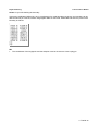
Chapter 3: Tutorial
3.1 Introduction..........................................................................................................................................3-3
3.2 Setting up a Triwaco project ...............................................................................................................3-4
3.2.1 Definition and preparation............................................................................................................3-4
3.2.2 Definition of a Triwaco Project.....................................................................................................3-4
3.3 Setting up a calculation grid ...............................................................................................................3-6
3.3.1 Step 1: Opening a Grid data set..................................................................................................3-6
3.3.2 Step 2: Defining the model boundary ..........................................................................................3-7
3.3.3 Step 3: Defining the position of watercourses (line elements) ....................................................3-8
3.3.4 Step 4: Defining the position of sources (fixed nodes)................................................................3-9
3.3.5 Step 5: Defining the position of node density areas ................................................................. 3-10
3.3.6 Step 6: Generating the grid........................................................................................................3-11
3.4 Setting up an Initial data set, the conceptual model setup ................................................................3-13
3.4.1 Opening an Initial data set.........................................................................................................3-13
3.4.2 Input of parameters covering the whole model area (type ‘node’) ............................................3-15
3.4.3 Input of parameters for watercources (type ‘river’) ...................................................................3-17
3.4.4 Input of source data (type ‘source’)...........................................................................................3-18
3.4.5 Input of boundary conditions (type ‘boundary’)..........................................................................3-19
3.5 Setting up a calibration data set (first calculation).............................................................................3-20
3.5.1 Opening a calibration data set...................................................................................................3-20
3.5.2 Allocation of data to the grid......................................................................................................3-21
3.5.3 Viewing and checking allocated data with TriPlot......................................................................3-21
3.5.4 First simulation...........................................................................................................................3-24
3.5.5 Viewing and presenting results..................................................................................................3-25
3.5.6 Comparing simulation results with measurements (calibration)................................................3-26
3.6 Setting up a Final data set.................................................................................................................3-27
3.7 Setting up a Scenario data set...........................................................................................................3-28
3.7.1 Opening a scenario data set and run a scenario simulation......................................................3-28
3.7.2 Combining and processing of model results and parameters...................................................3-29
3.8 Setting up a Pathline data set............................................................................................................3-31
3.8.1 Opening a Pathline data set.......................................................................................................3-31
3.8.2 Calculate pathlines from (abstraction) wells..............................................................................3-32
3.8.3 Calculate pathlines from user defined starting points................................................................3-33
3.8.4 An influence area calculation.....................................................................................................3-34
3.8.5 Interactive pathline calculation in TriPlot....................................................................................3-35
3.9 Setting up a Transient data set..........................................................................................................3-37
3.9.1 Opening a Transient data set....................................................................................................3-37
3.9.2 Defining user defined stress input (abstraction well).................................................................3-38
3.9.3 Defining input by time series allocation (precipitation excess).................................................. 3-39
3.9.4 Defining a time series ouput file.................................................................................................3-40
3.9.5 Running the Transient simulation..............................................................................................3-41
3.9.6 Viewing results...........................................................................................................................3-41
Annex 1: Lay out file defining the boundary
Annex 2: Lay out files defining the sources
Annex 3a: Application of the parameter allocators
Annex 3b: Proposed default parameter values for demo-model
Annex 4: Lay out calibration file (measured heads)
Annex 5: Lay out time series files
Annex 6: Exercises
Royal Haskoning
Triwaco User's Manual
3.1 Introduction
There are several possibilities to get to know Triwaco. The most extensive information on the software
package can be found next chapters of the manual, that includes not only an explanation of how to run the
software, but also contains extensive background information of the different modules. This information can
also be accessed by the Help function in the TriShell.
This tutorial gives an introduction to Triwaco, meant for those who are familiar with groundwater modelling
and wish to get a quick view of the normal method to set up and to run a groundwater model, and the
standard possibilities of Triwaco. A complete view is obtained by using the manual.
The model set up in this tutorial will be located in the directory C:\My Models\Demo. All data referred to in the
text is available in the directory C:\ My Models\Demo\Topo.geg. A resulting version of the model is located in
the directory C:\My Models\Tutorial. So when things go wrong or you don't know what to do one can always
refer to this working model. Below an overview of the succesive steps of building a model in Triwaco is
given. This is in fact the standard method by which a model is set up.
1 Setting up a Triwaco project
2 Setting up a calculation Grid
3 Setting up an Initial data set, the conceptual model setup
4 Setting up a Calibration data set (first simulation)
5 Setting up a Final data set
6 Setting up a Scenario data set
Additional steps may include solute transport, transient or other calculations. In this tutorial two often occuring
additional calculations will be explained.
- Setting up a Pathline data set
- Setting up a Transient data set
3 Tutorial-3
Royal Haskoning
Triwaco User's Manual
3.2 Setting up a Triwaco project
Now we show you the steps to take for making a groundwater model using Triwaco. We keep to the ‘main
route’; extra options are mentioned with the letter E and shown in italic. Important notices are indicated with NB.
3.2.1 Definition and preparation
Model building starts with the choice of boundaries and collection of data. This is done without the use of the
software, and will not be discussed here. We advise you to make a topographical background map that will help
you orientate while using the digitising and presentation modules of Triwaco. A background map can have
different formats (such as bitmap (*.bmp), ArcInfo-ungenerated (*.ung) and DXF). A simple alternative is to
make a rectangular grid of (e.g.) kilometers (see Annex 1).
An example of a background map is available after installing TRIWACO on your hard drive.
The file is located in the directory c:\My Models\Demo\Topo.geg\. The bitmapfile can be used in either the
digitising module or the presentation module.
Triwaco works with a clear hierarchical data storage structure. The entry always is a project that can contain
several models. Every model consists of different connected data sets that contain different parameters.
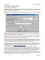
3.2.2 Definition of a Triwaco Project
Modelling with Triwaco always starts by defining a project.
'Project' 'New' if you set up a new model, otherwise 'Open' - and look for the name of your project), type a name
of the project.
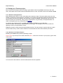
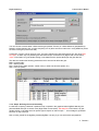
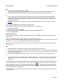
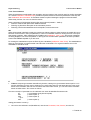
You now see the start window in which the different data sets are registered.
3 Tutorial-4
Royal Haskoning
Triwaco User's Manual
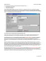
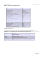
The data sets shown above will be created during this course and so this window will be filled with data sets
during the model building. The project window displays the following information.
Type
Grid
Based on
Transient
Phreatic
Var. dens.
Description
Subdirectory
Description of type of data set.
Finite Element or Finite Difference grid to be used for calculations
Data set with (hydrogeological) parameters to which this set refers
Indicates whether or not transient calculations are carried out
Indicates whether or not the uppermost aquifer is phreatic
Indicates whether the variable density module is used
Descriptive commentary of the data set and its use
Name of the subdirectory for this data set
In the top left corner is a button to start the note editor. Anything you wish to comment on your model can and
should be attached to the model by using this option. This button is available for each data set. Each data set
has its own comment-file.
E
It is possible to use your favourite text editor, instead of the standard Windows notepad. To do this Lm
Tools in the taskbar at the top. Lm TriShell programs. Fill in the path of your favourite text-editor or browse
by using the browse button. Lm ok, or if you have second thoughts Lm cancel.
3 Tutorial-5
Royal Haskoning
Triwaco User's Manual
3.3 Setting up a calculation grid
The calculation grid is set up in 6 steps. The following items need to be defined:
1.
2.
3.
4.
5.
general data
boundary
linear surface water or other line elements (faults for instance)
position of sources
position of density areas
When these items are defined the grid can be generated (step 6).
3.3.1 Step 1: Opening a Grid data set
The data for the generation of a calculation grid are treated as a data set. You’ll need: the positions of the
boundary, the linear surface water that you want to include in the model and the sources (the grid is taking
these elements into account) and specified sub-areas with a certain density of the calculation grid. These data
are entered successively.
Add the data set: 'Data set','Add','Grid', as shown below.
E
In this tutorial a finite element grid is used. It is also possible to make use of a finite difference grid
(ModFlow). Setting up a finite difference grid is carried out in the same 6 steps described in this tutorial.
NB
The names of the data sets are used to make directories. Spaces and points are allowed in the names of
files and directories in the 32 bits windows versions (from Windows 95).
3 Tutorial-6
Royal Haskoning
Triwaco User's Manual
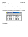
You can choose to create either a finite-element grid (default, Triwaco) or a finite-difference grid (ModFlow).
Default is a finite-element grid, so leave everything as it is (there are some restricions in using ModFlow). Enter
the name of the grid (in this case Grid).
A data set in Triwaco can be opend in ways. The first is selecting the data set and then from the menu 'Data
set','Open'. A faster way is by selecting the data set and open a context menu (Right hand mouse button),
'Open'. Even faster is by just double clicking on the data set to be opened. Now open the grid data set.
The data set contains the following parameters which are used to define the grid:
BND = grid boundary
POL = density areas
RIV = linear surface water (brooks, canals, rivers) or other line elements (faults, etc.)
SRC = sources (wells)
3.3.2 Step 2: Defining the model boundary
Lm Simular to opening a data set a paramter map is opened in the graphical editor DigEdit. Selecting the
paramter BND and open a context menu (Right hand mouse button), 'Edit Map File'. Even faster is by just
double clicking on the data set to be opened. Ignore reports as 'Cannot open ..' , this message is generated
because no map exists yet.
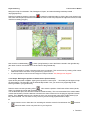
Now you find yourself in the digitising module (DigEdit). It is easy if you can work with a topographical
3 Tutorial-7
Royal Haskoning
Triwaco User's Manual
background map for orientation: 'File','Background','Open', and select de backgroundmap located ..
\topo.geg\topo.bmp.
Draw the boundary by drawing a polygon (
) Create the model boundary by clicking the corner points in the
area; enter the last point (that doesn’t need to be the same as the first point!) with the right hand mouse; this will
close the boundary (polygon).
Now save the modelboundary (
). Check (using Browse) to see if the files are stored in the right directory
(the name of which must be the same as the name of the grid data set).
E
It is also possible to create a boundary with exact coordinates. This can be done by creating a file named
‘BND.UNG’ with a text-editor in the grid-directory (see Annex 1).
It is also possible to load a second background map as follows: 'File','Background','Append'.
3.3.3 Step 3: Defining the position of watercourses (line elements)
Open de RIV parameter in DigEdit. Again ignore reports as 'Cannot open ..' . Now load your background map
as shown before. The boundary map is automatically loaded. If not, you can do so by appending the file
bnd.ung located in your grid directory.
Draw the water courses by drawing a line (
) . Now enter the position of the linear surface water (canals,
rivers), by clicking the corner and connection points.
You are allowed to place line element outside the model boundary. This is recommended if the surface water
crosses the boundary. Each line element is closed in the same manner as for the polygon (right hand mouse
button). Then Triwaco presents you a window in which you can enter the name of the surface water (if you
like). Save the data. You can enter as many rivers as you like. Simply repeat the above steps.
E
Delete a water course: Select the river activating the selection mode for line-elements: first
and then
,select the water course and press Del on your keyboard.
3 Tutorial-8
Royal Haskoning
Triwaco User's Manual
Select the river activating the selection mode for line-elements: first
watercourse.
Move a point of a water course:
,
. Undo: Ctrl-Z or
lines are visible select 'Options,'Show Vertices'.
Print the map using File/Print or the well-known icon
and then
, drag the
or 'Edit', 'Undo'. When no points on the
.
3.3.4 Step 4: Defining the position of sources (fixed nodes)
Open de RIV parameter in DigEdit. Again ignore reports as 'Cannot open ..' . Now load your background map
as shown before.
Now enter the position of the sources (
). Everywhere you click in the area a source is placed. DigEdit will
open a window in which you can enter the name (or code) of the source. After which you can carry on an enter
a new source. Make sure that the sources are not placed outside the model boundary. You can change the
name of sources by: Select the river activating the selection mode for line-elements: first
and opening the the context menu for that particular source.
E
and then
,
If you have the geographical co-ordinates of the sources beforehand, you can create the source data files
with an editor; see Annex 2. Save these files in the grid directory.
For grid generation and better description of groundwaterflow near sources is possible by appending
support circles. These circles are created in the Grid data set as follows: G
' rid','Define support circles'.
3 Tutorial-9
Royal Haskoning
Triwaco User's Manual
3.3.5 Step 5: Defining the position of node density areas
Open de RIV parameter in DigEdit. Again ignore reports as 'Cannot open ..' . Now load your background map
as shown before.
If you wish, append the maps of the linear surface water and the sources that are stored in the grid directory
with the file names ‘RIV.UNG’ and ‘SRC.UNG’ (see Step 3).
Now we will enter the zones with which the node densities are defined for the calculation grid; these are called
‘density areas’. The boundaries of these density areas are entered in the same way as the model boundary by
definition of polygons (see Step 2). After closing each boundary, a window pops up with the request to 'Enter ID
and value'. Enter the required node distance of the (selected) density area in the field ‘Value’ (usually in
meters).
For changing, deleting or moving a density polygon click the icon
polygon) or
first, and then
(to start editing the
(if you want to move a vertex). To change node distances: select the polygon by clicking the
icon
first, and then
, and change the value. Deleting polygons can be done by: select the polygon
and press Del on the keyboard.
You can change the entered node distances quickly by using an editor: Lm POL, Rm POL, Lm Edit par file. A
list will appear of the density area ID numbers and the entered node distances. Save the file and return to the
data set.
NB
The polygon of the last area must be placed completely outside the model boundary.
If you move the corner point of a density polygon where the boundary was closed (i.e. the first corner point
entered), you may risk to open the boundary. In that case, delete the line and enter a new polygon.
3 Tutorial-10
Royal Haskoning
E
Triwaco User's Manual
Adding a vertex to a line/vertex can be accomplished by selecting a line or polygon and then 'Edit', 'Add
Vertex' or just by using the Insert key. Then you can indicate the location of the vertex to be added.
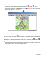
3.3.6 Step 6: Generating the grid
Now all data is entered, the grid can be generated.
If the model is going to be used for pathline calculations, adding support circles to the source nodes is
recommended though not necessary. Add support circels by: 'Grid', 'Define support circles'.
To generate the grid: 'Grid', 'Generate input file' and then 'Grid', 'Start grid generation'. An error message may
appear due to incorrect input. In this case repeat the above steps.
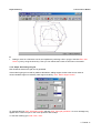
To view the resulting grid: 'Grid','View', 'Grid'.
3 Tutorial-11
Royal Haskoning
Triwaco User's Manual
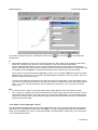
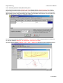
Now you have entered the presentation module Triplot. You can zoom in and out to check the grid with the
well-known icons:
E
. Leave the presentation module and close the grid data set.
Visibility of parameters (like elements, nodes, rivers) as well as the appearance of parameters can be
changed in the properties window (Lm or View',' Properties form the pull down menu will open the
properties window).
3 Tutorial-12
Royal Haskoning
Triwaco User's Manual
3.4 Setting up an Initial data set, the conceptual model setup
The conceptual model is defined in the Initial data set. This data set contains the inputparameters needed to
run the model. The data in this data set is independent from the grid and can be compared to shape files
used in a GIS. The characteristics of each parameter are entered using maps which may contain point
values, polygons, lines or constants or a combination. The parameters may also depend on each other using
expressions. The default length and time units are meters and days.
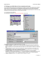
3.4.1 Opening an Initial data set
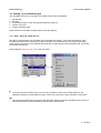
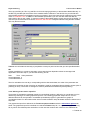
The initial data set is opened by: 'Data set','Add','Initial data', shown below.
In the definition screen you must define initial data for the model:
name for this data set: usually Initial. The names of the data sets are also used to make directories.
phreatic conditions: if chosen, the model will calculate with a variable transmissivity of the first (top)
aquifer, depending on the groundwater head in this aquifer. We will use phreatic conditions so check this
one.
variable density: this option is used when calculations are carried out whereby the groundwater has a
variable density (this option will only work with the Variable Density module which is not available in the
standard package). In this model no variable density is used.
top system number: type of topsystem (see manual for an explanation of the various Triwaco
topsystems). In this case select topsystem no. 11. This type of topsystem is releatively simple and is often
used, it contains precipitation excess, drainage and infiltration resistance and a controlled waterlevel.
number of aquifers (obvious). The model will contain 2 aquifers so select 2.
3 Tutorial-13
Royal Haskoning
Triwaco User's Manual
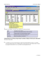
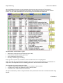
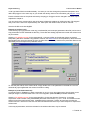
After this Triwaco will present a list of parameters whose values need to be entered. The amount of
parameters and the type of the parameters are based on the initial settings chosen in the former definition
screen. You can sort the parameters in the list by clicking one of the titles in the table head.
The parameters can be divided in 4 types:
parameters covering the whole model area (type 'node')
linear surface water parameters (type 'river')
source parameters (type 'source')
boundary conditions (type 'boundary').
Every type has a specific way of definition, which is made clear in the next paragraphs.
Within this initial data set all parameter information is stored. In other words this data set is your databank for
maps which are independent from the modelling grid and can later be used for other models.
The information is stored in three types of files:
.ung files, (ungenerated file) which contain the co-ordinates of the map items.
.par files, which contain the parameter values of the map items.
.nam files, which contain the names of the items .
All maps are defined by at least an ungenerated file and a parameter file which can be viewed and edited using
Digedit.
3 Tutorial-14
Royal Haskoning
Triwaco User's Manual
NB (initial settings)
The names of the data sets are used to make directories.
The next time you open the definition screen you can change the data set description.
If you want to change one of the initial settings, delete the data set in the list of data sets and start again:
Select the data set, 'Data set' , 'Delete'.
3.4.2 Input of parameters covering the whole model area (type ‘node’)
The following parameters are node type parameters:
Parameters that define:
The topsystem (parameter code RPn.),
The resistance of the aquicludes (CLn.)
The transmissivity of the aquifers (TXn.) or the permeability (PXn.),
The top level of the first aquifer (RL1)
And optionally the base level of the first aquifer (TH1).
The data to be entered for the different parameters are listed in annex 3b. To help you enter the data three
examples are explained in more detail below. In this case two topsystem parameters, but the way the data is
entered applies to all data covering the whole model:
1. The precipitation excess (RP1) is, in this case, entered with ‘polygons’ (areas with a constant parameter
value) and a default value for areas where no value is defined.
2. Surface level (RL1) is defined by point values which may be entered using DigEdit.
3. The average water level in the small surface water (ditches etc.) (RP5) that is related to the ground level.
Example 1 (precipitation excess):
In the Initial Data set open the Info definition screen of the paramter RP1. Open the conctext menu (Right hand
mouse button) and select 'Info'.
Enter a default value (in meter/day, e.g. 0,001 m/day = 1 mm/day). You can choose different allocators
depending on the type of input (see Annex 3a). In this case, for polygons, select Arpadi. The parameter is of the
3 Tutorial-15
Royal Haskoning
Triwaco User's Manual
‘node’ type that is filled in as default already. You want you can also change the parameter description. Now
define the polygons in the same way as you did with the density areas of the calculation grid (see par. 3.3.5).
Enter the desired value of the points enclosed by the polygon. Polygons can be changed in the same way as
explained in chapter 3.
You can check at any moment which part of the area is filled with isoplanes by clicking the item ‘Fill polygons’
that you find in the sub-menu Options/Setup; the ‘white spots’ will remain white, the rest is coloured.
Save the file RP1 and close DigEdit.
Example 2 (surface level):
In the directory topo.geg two files mv25.ung (coordinate-file) and mv25.par (paramater value file) can be found.
Copy these files into the initial data set directory. These files are already prepared and contain the surface level
as point values.
Open the 'info definition screen' for the parameter RL1. Choose InvDist as the allocator (there are several
interpolating allocators available using different methods, see annex 3a for a short explanation). Next select the
appropriate mv25.ung and mv25.par file from the initial data set directory. Note that the parameter filename not
necessarily has to be equal to the parameter name.
To view the point values of the surface level, simply double click on the parameter in the data set. This will
automaticaly open DigEdit with the surface level file for editing.
Example 3 (controlled waterlevel):
A powerful option in Triwaco is to base a parameter on one or more other parameters. We will show you an
example using the controlled water level. This is the topsystem parameter RP5 (controlled waterlevel).
Open the 'info definition screen' for the parameter RP5. Choose the allocator ‘Expression’. In the field
‘Expression’ enter a relation using the Triwaco parameter code names, e.g.: RL1 – 0.80. This relation means
that the level of the small surface water, modelled with the topsystem, is taken at a level 80 cm below the
surface level RL1. Note that in this case it is assumed that the level of the top of the first aquifer is equal to the
surface level.
In this way all parameters, which are relevant for the whole model area, may be entered.
3 Tutorial-16
Royal Haskoning
Triwaco User's Manual
NB
The code names are always typed in capitals.
The polygons may overlap. A grid node that is situated in two planes will be given the parameter value
belonging to the polygon with the smallest area (the polygons are sorted by the allocator Arpadi).
E
If corner points of the isoplanes are placed close to each other, it is possible that the graphical editor will
merge (‘snap’) the points. All points within a standard ‘snap distance’ will be merged. You can change the
snap distance in the submenu Options/Setup/Snap options or you can turn off snapping completely (see
check box 'Snap nodes').
Expressions can get as complicated as you desire, an example: IF(RL1>TH1,RL1,TH1+0.01) (See also
annex 3a).
3.4.3 Input of parameters for watercources (type ‘river’)
The parameters of the linear surface watercources (brooks, rivers, canals) are:
1.
2.
3.
4.
The water levels HRn.
The width of the water course RWn.
The resistance for exchange of groundwater and surface water CDn. and Cin.
The river activity RAn.
Example (water level):
As an example we take the parameter defining the width of the rivers (HR1). We enter the parameter values
using a map.
Open the info definition screen for the parameter. Choose the allocator parriv.
Now open the HR1 mapfile in DigEdit. Next step is adding the surface water map that previously made for grid
generation: 'File','Append'. Look for the file 'RIV.UNG' in the grid directory.
Mind the fact that you did not open this map as a background map this time! Instead you opened it to perform
operations on it.
NB
E
Each watercourse must be given at least one value (entered by one linked point).
The linked points do not need to be placed exactly on the watercourse; a short distance from it will work too.
If the value changes within a short distance (e.g. over a weir), then you place the linked points at the start
and end of this short section.
The River Activity (RA..) is a special parameter, that is a value (0 (inactive) or 1(active)) (see below).
Linked points are stored in a different way as stated in chapter 3.1. In this case the river number to which
the point is linked, the coordinates as well as the parameter value are stored in the ungenerated file (e.g.
HR1.ung)
The values of the river parameters are defined by so-called 'linked points'. These linked points are placed on, or
within a short distance of, each watercourse. The allocator interpolates between these points, or extrapolates
outside these points. Now enter the position of the linked points (
). For each point you will be asked for a
line to be linked to and a value. Choose as link the ID of the watercourse, and enter the parameter value. The
ID of the linked point is not important.
If the watercourse numbers are not shown on the screen, change it in the menu Options/Setup/Label: Ids (and
not: Hide labels).
3 Tutorial-17
Royal Haskoning
If you wish to change the value of a linked point: click the icon
linked points)
E
Triwaco User's Manual
first, and then
(to start editing the
By default the watercourses are active in the first aquifer only; the number in the parameter codes (HR1)
marks this. If a watercourse works in a second aquifer too, you must add some parameters:
Choose Parameter/Add/Internal, and look in the parameter list for the parameter type: 'River activity in
aquifer', select this type. The parameter is added to the data set with the code name RA. Change this in the
info definition screen to RA2 (the ‘2’ indicates that the parameter is related to the second aquifer).
Do the same for the other parameters: HR ('Water levels in rivers in aquifer'); RW ('River widths in aquifer'),
CD ('Drainage resistance of rivers in aquifer') and CI ('Infiltration resistance of rivers in aquifer'); add a ‘2’ in
all cases. Then you enter the values.
The water level (HR2) may be taken equal to the level in the first aquifer (HR1). In the info definition screen
you choose as an allocator ‘Expression’, and enter the relation in the field ‘Expression’: HR1 (which means:
HR2 = 1.0 * HR1). The other parameters can be treated in the same way, or you can enter new values
using a map.
NB
If you do not enter a value in a map, the default value is taken (defined in the info definition screen).
On a confluence or division point of two watercourses you need to enter values for each of the two. As you
cannot stack the input points, you put the points on (or next to) the watercourse, at a short distance of the
confluence or division point. If the points are merged, change the Snap distance (see par. 3.2), delete the
points and enter them again.
3.4.4 Input of source data (type ‘source’)
The source data are entered with the help of the graphical editor too. You can choose between sources with a
fixed abstraction rate (parameters with code name SQn.) or a fixed head (parameters with code name SHn.).
Either one is activated by the value of the parameter ISn.; the default value is 0 (fixed rate); if you enter value
of 1 a fixed head is expected.
3 Tutorial-18
Royal Haskoning
Triwaco User's Manual
Example (abstraction in aquifer 2):
As an example we take the sources in the first aquifer defined by the parameter SQ2 (sources in aquifer 1 are
entered by parameter SQ1 etc.).
Open the info definition screen for the parameter. Choose the allocator srcparado.
Now open the SQ2 mapfile in DigEdit. Now open the source position map that you created for the calculation
grid by appending the file SRC.UNG located in the grid directory.
Assign the abstraction rate for each source in the Value field (in m3/d, negative number in case of an
abstraction, positive in case of an injection) and enter a description if you want.
E
Input is also possible using an editor, see Annex 2.
3.4.5 Input of boundary conditions (type ‘boundary’)
The parameters for boundary conditions are:
Type of boundary condition (0 = fixed head, 1 = flux), IBn.
Boundary head, if boundary condition is a fixed head), BHn.
Parameters to determine a flux over the boundary; both 0 in case of a flux=0; see the manual for other
possibilities, BAn. and BBn.
The boundary conditions are entered with linked points, similar to the parameters for the linear surface water. In
DigEdit append the boundary map (File/Append) that is stored in the grid directory with name BND.UNG. The
linked points by definition always are linked to 1, since there is only one boundary.
In this demonstrationmodel the boundary condition is a fixed head, which means that IBn=0.
Consequently you only need to enter values for the head (parameter BHn). The other parameters remain zero.
The values are entered similar to those for linear surface water. Inbetween linked points the values are
interpolated. To keep the model simple enter a constant value for the boundary head of 0.5m.
NB
If the type of boundary condition (fixed head / flux) should be different at a certain location or stretch of
boundary, put two points with different values for IB at both sides of this location (=grid node).
3 Tutorial-19
Royal Haskoning
Triwaco User's Manual
3.5 Setting up a calibration data set (first calculation)
Up to now the parameter values are stored independently of the calculation grid in tables and maps. The
advantage is that the grid can be changed without a change of the original input. The original input is linked
(allocated) to the grid in a separate data set, the calibration set. This is done only for the conceptual model and
the calibration; for scenario calculations the changed basic data (maps and tables) and with their allocated
values are stored in the corresponding scenario data set.
3.5.1 Opening a calibration data set
The calibration data set is opened by: 'Data set','Add','Calibration Set'.
Enter a description (preferably without spaces or points).
3 Tutorial-20
Royal Haskoning
Triwaco User's Manual
The Calibration data set is based on the Initial data set; this is shown in the next input screen (see the name
in the field ‘Based on’). If you have more than one calculation grid you can choose one in the field ‘Grid’.
Triwaco will show the list of parameters of the initial set. Currently all parameters have a red cross which
means they either need to be updated or allocation is not carried out yet. We will now allocate them to the grid.
3.5.2 Allocation of data to the grid
Allocation is done as follows:
per parameter: select the parameter, open context menu (right hand mouse) and select Allocate (shown in
the picture below).
for a group of parameters: select the group of parameters and Allocate.
The parameter information, defined by polygons, lines or points, is translated to so called adore files. An adore
file has a fixed format in which the information for each grid node is stored. These files have the extension .ado.
NB
If parameters are related to other parameters by means of an Expression, the independent parameters
must be allocated first and the dependent parameters after that.
There is always a change of error in the input files. It is therefore recommended to check all the allocated data
(adore files) before running a simulation! The easiest way is to use the presentation module Triplot. However,
you can get a quick view of an allocated input file if you select the parameter, and 'View Ado file as text', but you
will only see columns of numbers. The use of TriPlot to view data input that is allocated to the grid will now be
explained.
3.5.3 Viewing and checking allocated data with TriPlot
To view a parameter in Triplot, select a parameter and 'view Ado file'. The presentation module Triplot is
opened. After the first parameter is loaded into TriPlot you may select multiple files from the data set and load
them at once into TriPlot.
NB
If you want to see another file, choose (in TriPlot) 'Parameter','Load'. Select the paramter file and the
parameter set. Choose 'Info' for some statistical information.
E
Visibility of parameters as well as the appearance of parameters can be changed in the properties window
(via the context menu or by selecting 'Properties form the pull down menu)
3 Tutorial-21
Royal Haskoning
Triwaco User's Manual
You can present the parameter values in several ways:
- Isolines
- Classes
- Node values.
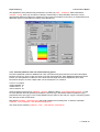
Isolines
Choose 'Param','Contour', select the parameter. An input screen will appear. The commands in the corner left
below (Level) are the most important. A default set of isoline values (levels) has been filled in already, from the
minimum to the maximum parameter value.
Change the total set using Level. You’ll get equal differences between the isoline values.
Change an individual level using Modify; the value and the colour can be changed, and the colour too (click
the coloured field to change the colour).
Change the default series of colours using Colour (command right of Level).
Insert a level by clicking Insert; Delete will delete a level.
If you want to save a set of levels, choose Save and enter a file name with the extension 'lvl'.
Load the saved set of levels using Load.
Default restores the original set of levels.
See the manual for the other possibilities of TriPlot.
If absent add a legend choosing 'View','Legend' and the parameter shown. If you want to change the isolines,
you can do so by 'Param','Contour' or 'View','Properties'.
Classes:
The definition of classes is nearly the same as the isoline definition. Choose 'Param','Classify', and do the same
as described here before for isolines. If you want to change the classes, you can choose 'Param','Classify' or
'View','Properties'.
NB
The numbers in the input table are always the upper limits of the classes. A number equal to a limit is
classified into the class with higher values. So, if you enter class limits -1 0 1 2, the classes will be:
1. [x < -1] ; 2.[-1 <= x < 0] ; 3. [0 <= x < 1] ; 4. [1 <= x < 2].
3 Tutorial-22
Royal Haskoning
Triwaco User's Manual
Node values:
You will frequently use the properties window 'View','Properties' (or click righthandmouse button somewhere in
the map). The left part of the window is a list of items shown on the screen; the right part gives a list of all
other items that are hidden. You will find - among others - the node values of the chosen parameters ('Node
labels').You can also select an item in the list of Visible items, and change the appearance.
Some other options:
Enter a background map in the menu 'View', 'Background map', similar to loading a backgroundmap in DigEdit.
One may for instance also load a parameter input map to check the allocated parameter. The parameter maps
can be found in the Initial data set directory; it’s a file consisting of the code name of the parameter and the
extension .ung.
E
An extra dimension to the presentation of parameters can be given by the option 'Parameters','Shading'.
Measure lengths and areas by selecting
, and pointing the corner points by clicking in the map. The
lines will remain on the screen until you zoom in or out or rewrite the screen in another way.
Cross-sections can be made by selecting
, and pointing the corner points of the section by clicking in
the map. To end a section click the righthand mouse button. Experiment with the options in the section
window. Best results are obtained when layer parameters RLn and THn are loaded in TriPlot as well.
Try the inspector
. Pointing and pressing the left-hand mouse button at various locations causes the
program to display coordinates, element and node numbers and values of all loaded parameters for the
selected location.
When contouring parameters, try the option of transparency
NB
If you have loaded more parameters after each other with the same name, a serial number is added to the
code name.
When more than one paramter is contoured/classified you can change the order of appearance similar to a
GIS system in the properties window.
If the parameter must be modified do so in the Initial data set. Select the parameter, and modify it like you did
before entering the parameter values. After that, go back to the Calibration data set, and allocate the parameter
again!
3 Tutorial-23
Royal Haskoning
Triwaco User's Manual
3.5.4 First simulation
When all parameters are allocated to the calculation grid and checked, the model is ready for the first simulation
run. Choose 'Calibration','Generate input' (creates an inputfile, based on the actual parameters in the set) and
then 'Calibration','Run Simulation'. A simulation window is opened showing the progress of the simulation.
When ready it closes. You can now view the results.
When a simulation is finished the following files are produced (located in ..\Calib1):
Flairs.flo: result file with piezometric heads and fluxes
Flairs.flg: log file with a description of the calculation process
Flairs.flp: print file with waterbalances for all aquifers, rivers and sources
NB
When all input data is defined correctly the model runs without problems. Often however the model will not run
because of some errors in the input parameters. There is no standard method for finding the error in the input
that causes a problem. Often reading the file FLAIRS.LOG ('Calibration', 'View', 'Log'), where error messages
are being displayed, can solve the problem. In the log file it is recorded which parameter causes the problem.
Contact the Triwaco Helpdesk if you are stuck.
For viewing the waterbalances open the Flairs.flg into a texteditor ('Calibration','View','Print'). The waterbalances
show you how well the conceptual model is and thus the model itself is. For a good model the error in the
waterbalance should be small.
E
Triwaco computes groundwater heads/flow by iteration, starting from groundwater heads equal to 0.0. A
quicker calculation process may be obtained if you enter initial values for the heads that are closer to the
heads to be calculated. After the first calculation with reasonable results, you can enter these calculated
heads as initial values. This is done as follows:
First add a number of parameters to the calibration set under the Modified Parameters-tab:
HT
(= groundwater head phreatic aquifer)
HH1
(= head aquifer 1)
HH2
(= head aquifer 2)
... up to:
HHn
(= head aquifer n).
Adding parameters is done by:
1. Go back to the Calibration set','Modified tab, and choose 'Parameter','Add','Internal', and look for
3 Tutorial-24
Royal Haskoning
Triwaco User's Manual
‘Groundwater head in topsystem’. Select this parameter type.
2. In the parameter list of the data set, select the new parameter with code name HH, open the context menu
'Info',:
change the code name HH to HH1 (parameter refers to aquifer 1)
change the description to ‘.. aquifer 1’
choose as an allocator: Expression
type in the field ‘Expression’: 1.0 * PHI1. (PHIn for the other aquifers).
Close
3. Repeat action 1 and 2 one or more times (depending on the number of aquifers that are included in the
model). Always select the parameter ‘Groundwater head in aquifer’.
4. For the groundwater head in the topsystem, select the new parameter with code name HT, open the
context menu 'Info',:
choose as an allocator: Expression
type in the field ‘Expression’: 1.0 * PHIT
Close
5. Allocate the new parameters.
6. Note that this will speed up the iteration process.
3.5.5 Viewing and presenting results
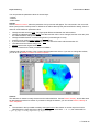
When the simulation is finished, you can view the results. Choose 'Calibration',View','Results'; again Triplot is
opened. The simulation results are automatically loaded, so you can directly select one of the output variables.
(If the output file appears not to be selected, Choose 'Param','Load', and select the file ‘flairs.flo’ in the directory
of the calibration data set. Then you can continue with the presentation of the results). Presentation and viewing
of the results is carried out in the same way as for viewing allocated data explained earlier.
The results consist of the following variables:
PHIT = head phreatic aquifer (in meter+ reference level)
PHIx = head aquifer x (m+reference level)
QRCH = recharge first (top) aquifer (m/day; positive = downward flux)
QKWx = recharge of aquifer x from aquifer below (m/d; positive = upward flux)
QRIx = exchange flux between groundwater and the linear surface water, in aquifer x (in m3/day; positive = from
surface water to groundwater).
3 Tutorial-25
Royal Haskoning
Triwaco User's Manual
3.5.6 Comparing simulation results with measurements (calibration)
For the calibration of the model you compare the results with measurements. In most cases a model is
calibrated using measured groundwater heads, but calibrating using fluxes is also possible. In Triwaco
comparison between measured and simulated results is automated. The only thing you have to do is to create
an calibration-input file which has a fixed format. The measured head should be entered in an ASCII-file named
calib.chi. In annex 4 it is explained how to make calibration input file. In the directory topo.geg a predefined
calib.chi can be found. Simply copy this file into the calibration data set directory. Go back to the TriShell and
view the file by 'Calibration','Calibration','Input'.
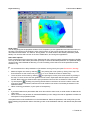
After a calculation the calculated and measured heads are compared automatically. The results (stored in the
file calib.cho) can be viewed choosing 'Calibration','Calibration','ViewOutput', or
'Calibration','Calibration','ViewMap' which opens TriPlot. You will be prompted to load the checkpoint output
from TriPlot. This is done by 'View',' Checkpoint Output'. Browse and locate and load the file calib.cho from the
calibration data set directory. Next the properties window is opened. If you like change the settings. The values
represent the difference of the calculated value with respect to the measured value. A negative value means
that the measured head is higher than the calculated head.
The result should then look something like this.
3 Tutorial-26
Royal Haskoning
Triwaco User's Manual
3.6 Setting up a Final data set
When you are satisfied with the results of the calibration, save the allocated input files and results in a separate
data set: the Final data set. You use this data set for scenario calculations to be based on.
The Final datset is created similar as any other data set. Choose ' Data set','Add','Final set'. In the field ‘Based
on’ you choose the Calibration data set. The input files (maps as well as allocated files) and results are copied
automatically to the Final data set. Close the data set.
NB
If you change a parameter in the Initial and/or Calibration data set the Final set is no longer up to date. In
that case update the Final set by opening it and choose 'Final',' Update'. The new input and output from the
data sets on which the Final data set is based on will then be copied to the Final data set.
3 Tutorial-27
Royal Haskoning
Triwaco User's Manual
3.7 Setting up a Scenario data set
In most cases a groundwater model is used to predict concequences of changes made to the water system.
These changes usually concern only a few model parameters. Therefor Triwaco has introduced the so called
Scenario data set. For a particular scenario data set the model parameters are enherited from the Final data set
(on which it is based) and only the parameters that need to be changed for that scenario have to be defined.
3.7.1 Opening a scenario data set and run a scenario simulation
When you want to add scenarios always remember to create a Final data set first (see previous chapter). For
each scenario simulation, open a new data set of the ‘Scenario’ type. Enter a name as done before. In the field
‘Based on’ you choose the reference data set 'Final'. Note that this can only be a Final data set.
You will notice that the dataset contains all parameters from the Final data set (and consequently from the
calibration dataset). These parameters are not physically present in the Scenario data set but are referenced to
the actual parameter files in the Final data set.
In the Scenario data set there are the tabs ‘Inherited’ and ‘Modified’. In the inherited-tab the parameters of the
reference data set are stored. In the modified-tab only the parameters that are modified with respect to the
reference data set are stored.
E.g.: if you want to calculate the effect of a different abstraction rate in a source, you only have to move this
parameter from the enherited tab to the modified-tab; the rest will be the same as in the reference data set. This
is done as follows:
Open the Scenario data set. Select the parameter(s) that are modified with respect to the Final set by choosing
'Modify Parameter' from the context menu.
Now the parameter is moved to the Modified-tab and the input parameters are copied from the initial set of the
reference data set. Notice that only the modified parameters will be physically present in the Scenario data set
directory.
Next modify the paramter by loading it in DigEdit. As explained for the initial abstraction rate in par. 3.5.4
change the abstraction rate for one of the sources. Save the paramter file and close DigEdit. Now allocate
this new data to the grid. You've now created an Scenario.
To run the simulation choose 'Scenario','Generate input' (creates an inputfile, based on the modified
parameters in the set and the parameters referenced to the Final data set) and then 'Scenario','Run
Simulation'. A simulation window is opened showing the progress of the simulation. When ready it closes. You
can now view the results with 'Scenario','View','Results'.
3 Tutorial-28
Royal Haskoning
Triwaco User's Manual
For practising the things you have learned in the former chapters, execute exercise 1 and 2 in annex 6. For a
little help on how to modify parameters, presenting the results and in an efficient way combining and
processing of data read the next paragraph.
3.7.2 Combining and processing of model results and parameters
You can combine and process data files in Triwaco; subtract, add, multiply or divide input data with input,
output with output and input with output. The result is a new parameter (user defined) that is stored in one of the
data sets (or a specially opened data set).
The parameters defined for processing have to be defined in one of the data sets (except grid and initial data
set since no adore files are present). For processing, add a parameter in one of the data sets under the tab
Modified. Choose 'Parameter','Add','User defined'.
Triwaco presents an input screen. Enter:
name: a codename (It is better not to make the code name longer than 4 characters, for Triwaco only
reads the first four. Do not make the name equal to existing code names, such as PHIT, RL1, RP1 etc.)
description: (obvious)
expression: insert the expression. If the parameters in this process are part of other data sets than the one
to which this parameter is added, you should specify the names of the other data sets. Always type the
name of the data set, a dollar sign and then the parameter code name (all without spaces), e.g.:
CALIB1$RL1 for the top of aquifer 1 in the data set CALIB1.
Example:
After calculating a scenario usually you want to determine the change in waterlevel with regard to the original
water level (stored in the Final data set).
Go to the modified tab of the scenario data set. Add a new parameter (Parameter','Add','User defined) called
dPHI2, (which is a possible abbreviation of difference between original and newly calculated groundwater
head).
Select the allocator to be ‘Expression’. In the field ‘Expression’ type: PHI2- FINAL$PHI2.
The parameter PHI2 is part of the data set to which the new parameter is added; that is why you do not have
3 Tutorial-29
Royal Haskoning
Triwaco User's Manual
to specify the name of this data set in the expression (it is the default set). Lm OK, and allocate the
parameter (Parameter','Allocate).
NB
The next time you do a simulation run with this scenario the difference is simply obtained by re-allocating
the parameter dPHI2.
A full explanation of the application of expressions can be found in the manual. A selection of often used
expressions can be found in annex 3a.
The resulting dPHI2 may look something like this. For other scenario simulations repeat the above described
steps, start by creating a new scenario data set.
3 Tutorial-30
Royal Haskoning
Triwaco User's Manual
3.8 Setting up a Pathline data set
3.8.1 Opening a Pathline data set
To calculate pathlines create a data set of the type ‘Path lines’ just like any other data set you have added until
now. In ‘Based on’ select the reference data set, for which you want to calculate pathlines. This can be a
Calibration set, a Final set or a Scenario set. In this case we will base it on the final data set.
The basic data of parameters from the reference set are given in the list with ‘Inherited parameters’.
Parameters that are specifically used in pathline calculations (which are not yet defined) are locateed in the
list with ‘Modified parameters’.
These parameters are the top and base of each aquifer as well as their porosity. These parameters must be
defined and allocated in the same manner as shown before. Two other parameters are TT, Top of topsystem
which is often chosen equal to the surface level (RL1) or the groundwater level (PHIT).
Through 'Pathlines ',' Options' a window is opened in which the type of pathline calculations can be selected.
The following types of calculations are discerned:
Tracing from wells
User defined starting points
Influence area calculation
It is also possible to carry out pathline calculations interactively in TriPlot.
Since it is often found difficult we will carry out all four possible ways of pathline calculations.
3 Tutorial-31
Royal Haskoning
Triwaco User's Manual
3.8.2 Calculate pathlines from (abstraction) wells
Open the options menu through 'Pathlines ',' Options'. Select the tab for 'Start tracing from wells'. For this
purpose copy the values from the picture below. In this window the well number is specified, the number of
pathlines used for the calculation, the depth from which the pathlines are started from and the starting angle
(almost always 0 which means horizontal). The length of the calculation is taken just as a very long period (in
days). The direction of the pathline is by definition upstream.
Next step is to generate the input file by 'Pathlines ',' Generate Input'. Which will generate the necessary files.
To start the calculation 'Pathlines ',' Run predefined',' Start tracing from wells'.
The result can be viewed by 'Pathlines ',' View ',' Wells ',' Streamlines'. De result may look something like this.
3 Tutorial-32
Royal Haskoning
Triwaco User's Manual
The appearance of the pathlines may be altered to your liking by 'View ',' Properties'. Select streamlines: ...
'\well.bin ',' Config'. Here you can select to classify in several ways. In the presentation above the colours
represent the different model layers. Instead one may choose for traveltime, fixed colour (no classification) and
destination (which is used often for influence area calculations).
3.8.3 Calculate pathlines from user defined starting points
First add a parameter under the 'Modified' tab. Give it the name XYZ (Only enter the name and a description
leave the rest as it is, since we are only going to use the ung and par file). Open DigEdit and add points at the
location you want pathlines to start from. As a value enter the depth from which the pathline has to start.
Remember always to choose a depth within one of the aquifers. For instance:
X-coor Y-coor depth
149042 409829 -40
148885 409717 -5
148134 409212 -40
Open the options menu through 'Pathlines ',' Options'. Select the tab for ' User defined starting points'. For the
XY value definition file enter (browse) and select the file XYZ.ung in the Pathline data set (otherwise copy a
prepared file from topo.geg). For the Z value definition do the same for the XYZ.par. Copy the remaining options
from the input screen shown below.
Next step is 'Pathlines ',' Generate Input'. Which will generate the necessary files. To start the calculation
'Pathlines ',' Run predefined ',' User defined starting points'.
The result can be viewed by 'Pathlines ',' View ',' User defined ',' Streamlines'.
3 Tutorial-33
Royal Haskoning
Triwaco User's Manual
3.8.4 An influence area calculation
An influence area calculation gives the area from which a well (in fact all wells), rivers (if draining) receive their
water from. For this calculation from every grid node from the surface level the pathway of the water is traced
downward to the well(s), rivers, seepage area or modelboundary. In other words until this water leaves the
model.
Open the options menu through 'Pathlines ',' Options'. Select the tab for 'Influence area calculation'.
To calculate influence areas (‘Influence area calculation’) a grid-file has to be defined (usually the model
network grid.teo in the grid directory) and the type of calculation (upstream/downstream/both) in this case select
downstream. The calculation starts by definition at the top of the system (defined through the parameter TT).
Next step is 'Pathlines ',' Generate Input'. Which will generate the necessary files. To start the calculation
'Pathlines ',' Run predefined ',' Influence area calculation'.
The result can be viewed by 'Pathlines ',' View ',' Influence area ',' Streamlines and MAPS'. This will load the
maps as well as all streamlines. Since we only want to view the influence area move the streamlines to the right
(invisible) in the properties window. Then load the file with the influence areas by 'Parameter ',' Load' then
3 Tutorial-34
Royal Haskoning
Triwaco User's Manual
browse (change the file type to *.tro) for infl.tro. Then select DESTINATION from the list. Then 'Parameter ','
Classify ',' DESTINATION'. The result may look something like this. You may also classify according to aquifer
or time.
The green colour (DESTINATION=0.5) shows infiltrations areas from which the water leaves the model at the
model boundary. The blue colour (DESTINATION=negative number of the river number) shows the influence
areas of the rivers. In yellow (well 2) and yellow/green (well1) the influence areas of the abstraction wells. No
influence area is calculated for well three since it is an injection well.
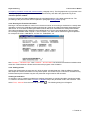
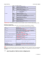
The destination code in the influence area output file (infl.tro) defines the character of the location of the end
point of the flow line. A negative integer indicates that the flow line ends in a river, with the absolute value of
the number being the river number or river ID assigned to that river. A positive integer indicates that the flow
line ends in a well, with the number being the source number or source ID assigned to that well. Other
destinations are indicated by a destination code with values between -1 and +1.
The next table summarizes the destination codes generated by the particle-tracking program Trace:
Destination
code
-1
-0.5
-0.4
-0.3
0.1 - 0.3
0.5
0.7
1
Description of destination
negative integer: number of river reached (c.f. grid.teo)
flow line leaving the system vertically (top-system reached)
flow line immediately leaving the system vertically:
upstream tracing in area with downward seepage (infiltration)
flow line immediately leaving the system vertically:
downstream tracing in area with upward seepage (e.g. a polder)
stagnant points reached
flow line leaving the system horizontally (crossing the model boundary)
maximum tracing time reached (time specified in the input file)
positive integer: number of source reached (c.f. grid.teo)
3.8.5 Interactive pathline calculation in TriPlot
Through 'Path lines ',' Interactive calculation' the presentation module Triplot is activated in which you can
interactively calculate pathlines. All the previous calculations can be carried out and, depending on the type of
calculation, more options are available.
To practise on pathlines execute exercises 3 and 4 of annex 6.
3 Tutorial-35
Royal Haskoning
Triwaco User's Manual
NB
- Through 'Path lines ',' Generate input' the input files for the (4) different types of calculations are generated:
Well.tri for pathlines starting from wells,
Trace.tri for ‘user defined’ starting points,
Infl.tri for calculations of influence areas and
Inter.tri for interactive pathline calculations in Triplot.
- Through 'Path lines ',' Run predefined' the defined pathline calculations (Well.tri, Trace.tri, Infl.tri) can be
executed. With 'Pathlines ',' View' the results are shown.
- After finishing the pathline calculations the following result files are produced:
.tro file, containing output of a trace calculation
.bin file, containing streamlines of a trace calculation
.lst file, containing the end points of a streamlines
.log file, containing the description of the calculation process and for every streamline the travelled time
and travelled distance is given.
Within Triplot select the option 'Trace','Streamline','Properties' to view the results for every individual streamline.
3 Tutorial-36
Royal Haskoning
Triwaco User's Manual
3.9 Setting up a Transient data set
3.9.1 Opening a Transient data set
For a transient simulation create a data set of the ‘Transient’ just like any other data set you have added until
now. In ‘Based on’ select the reference data set. This can be a Calibration set or a Scenario set. In this case we
will base it on the calibration data set 'Calib1'.
Next, transient options can be stated. Open the options menu by 'Transient ',' Options'. The follwing window will
appear.
The tab ‘Transient options’ concerns the definition of the calculation period. A start and an end-date can be
given as well as a stress input period. The stress input file consists of moments in time at which the system is
evaluated. These points need not to be equidistant in time.
Enter the start and end of calculation as given in the figure above. Select the Automatic stress input and enter a
timestep size of 10 days. (It is recommended to define integer values for the timesteps. This is because for
example the fluzo module does not handle real value timesteps well, yet.)
The tab ‘Calculation options’ concerns iteration options for the flairs-calculations and print options. For every
aquifer, including the top system, the user has to indicate which parameters he wants to be saved on every time
step. This is done under the pull-down menu ‘print option’. You can specify if you want the head in the aquifer,
the flux over the top and bottom of the aquifer, and the two-way fluxes to rivers and sources.
At the ‘Points for time lines’ the user can indicate for which locations the change in groundwater head will be
followed during the transient calculation. This will result in an ASCII-file, which can easily be imported into Excel
for example. This way you can create graphs of groundwater head against time. The use of this option is
explained in paragraph 3.9.4 Definition of a time series output file.
The basic parameters of the reference set are given in the list with ‘Inherited parameters’. Parameters
especially needed for transient calculations (which are not yet defined) are in the list with ‘Modified parameters’.
It concerns the elastic storage coefficients of the aquifers as well as the effective porosity of the top aquifer.
These parameters can be defined and allocated in the same manner as before. Enter a value of 0.001 for the
SC1 and SC2 (elastic storage coefficient) and a value of 0.3 for PE (porosity of the phreatic aquifer 1).
A transient calculation is executed because one or more parameters will change during a defined period of time.
The parameters are defined in the same way as in the former data sets. Parameters that will change during the
defined calculation period have to be moved to the tab ‘Modified parameters’.
3 Tutorial-37
Royal Haskoning
Triwaco User's Manual
A time-dependent parameter can be allocated in two different ways:
User defined stress input
Time series allocation
A user defined stress input is used when a parameter is changed only a few times during the simulated
period. For example controlled water level or stopping the abstraction from a well. Time series allocation is
used for parameters that change with (almost) every timestep. For example waterlevels in a river or precipitation
excess. In the following sections we will define both.
3.9.2 Defining user defined stress input (abstraction well)
In this case we will shut down the abstraction well number 1. This is in fact the same calculation as in the
formerly described scenario. This time however we will look at the change in water level through time.
By defining the input on the user defined stress input periods (‘Transient’ , ’Options’, see above), a parameter
can be switched on and off. In this way the abstraction rate before and after shutting down the well can be
defined. This can be done by the use of a tilde (~) within a parameter name. Triwaco will not read the
information, which is behind this tilde, but it will enable you to maintain different values for different periods of
time.
Define two different abstraction rates by adding two new parameters: SQ2~ON and SQ2~OFF. In this case
SQ2~ON is identical to SQ2 used in the steady state calculation. SQ2~OFF contains an abstractionr ate of 0 for
well number 1 since it will be shut down. By indicating the valid stress period for both parameters, Flairs will
read SQ2~ON for the internal parameter SQ2 for the situation whereby the well is still in use and SQ2~OFF will
be read for SQ2 when the well is not active. The two files can also be found in the topo.geg directory. Copy
them to the transient directory and reopen TriShell.
Next select SQ2~ON and open the 'Time Ruler' from the context window of by 'Parameter','Time Ruler'. Select
user defined stress inputs. Then mark the timesteps for which the SQ2~ON will be active. You only have to
mark the first timestep from a period in which the paramter is active. SQ2~ON is active untill it is deactivated by
the activation of SQ2~OFF. So only select 01/01/1997 as shown in the picture below.
3 Tutorial-38
Royal Haskoning
Triwaco User's Manual
Now select SQ2~OFF and again open the 'Time Ruler'. Select user defined stress inputs. Then mark the
timestep for which the SQ2~OFF will become active (that is when the abstraction is stopped). In this case on
the 12th of March 1997. So put a mark on this date. From this time on the SQ2~ON is deactivated andTriwaco
will use SQ2~OFF as the parameter SQ2.
Next allocate both parameters. Before that check the info is correct: Paramter type=source and
allocator=SrcParAdo. Before we start the simulation we will first define the precipitation excess.
NB
The SQ2 in the inherited tab will be ignored during the simulation since SQ2~ON and SQ2~OFF are defined in
the modified tab.
3.9.3 Defining input by time series allocation (precipitation excess)
By defining that the input is based on time series allocation, a measured time series is used (i.e. precipitation
excess). This time series has to be placed in a specified .tim file. An example of a .tim file is given in annex 5
and is included in the topo.geg directory.
The timesteps in the .tim file make up the stress periods. The standard way is that the parameter on each
timestep within a stress period is assigned the value specified in the .tim file. It is imported to note that dates
and times defined in the .tim file not necessarily have to correspond to time steps defined in the transient
simulation.
You can choose to either convert the values of the time series to intensities or to values to be converted to
averages. In this case we will use precipitation excess RP1 by converting time series to intesities. First move
the RP1 from the inherited tab to the modified tab as shown before. The 'Time Ruler' will appear. Select 'TIM
with parameter values to be converted to intensities', as shown in the picture below.
3 Tutorial-39
Royal Haskoning
Triwaco User's Manual
Then copy the RP1.par, RP1.ung and RP1.tim from the topo.geg directory to the transient dataset directory. In
the RP1.ung and RP1.par the location of the weather-station is defined. In the file RP1.tim you will find time
series relating amounts of precipitation excess to moments in time. Next open the Info windwo from the context
menu or 'Parameter','Info'. In addition to the standard specifications you can now also define the .tim- file.
Select the tim-file you just copied. To view the location of the weather-station simply open the file in DigEdit. To
view the input in text format of the tim-file 'Paramter','Edit TIM file'. Finally allocate RP1 using allocator InvDist!.
This may take some time.
Triwaco now calculates the intensity of precipitation excess per period of time that you have specified before.
NB
Another possibility is to convert to averages. In that case the time dependent values are averaged and
appointed to each time step. If you have the following .tim-file
Date
Time Value parameter
01/01/2002 00:00 5
11/01/2002 00:00 10
Then for calculation time t=2 days, corresponding with the date 03/01/2002, the value of the parameter is 6.
Important to remember is that conversion to intensities is used for parameters like precipitation excess (units X
(meters) per time). Conversion to averages is used for paramters like waterlevel (units X(meters)).
3.9.4 Defining a time series ouput file
Time series of simulated groundwater heads for user defined locations, defined by its coordinates, may be
obtained by defining a so-called graphnode input file. The resulting graphnode output file is a comma
delimited file and can be imported in a standard spreadsheet program to generate time graphs of
groundwater heads. For all locations after each successive iteration step calculated results are written to the
output file.
The graphnode input file is defined in the Transient options window under the Calculation options tabsheet. The graphnode input file is defined as a standard Triwaco map file, i.e. ungenerated graphnode.ung
file, by which user defined points are defined. In this case the locations are used from the calibration file
3 Tutorial-40
Royal Haskoning
Triwaco User's Manual
(Comparing simulation results with measurements, paragraph 3.5.6). The file graphnode.ung is present in the
directory topo.geg. Just copy this file into the Transient directory and define the graphnode.ung in the
Transient options window.
During the transient simulation Triwaco writes the calculated heads to a file called graphnode.out. The
processing of the point for time lines is explained in paragraph Viewing results (3.9.6).
3.9.5 Running the Transient simulation
Running a Transient simulation is carried out in the same manner as for running a simulation for a steady-state
calculation carried in the Calibration and Scenario data set. However the initial groundwater head needs to be
defined first. In most cases the initial groundwater head is defined as calculated in the steady-state situation.
The initial groundwater head is defined in the modified tab as HT for the groundwaterlevel in the topsystem,
HH1 as the groundwater head in aquifer 1, HH2 in aquifer 2, etc. Each can be defined through an expression.
For example HT will be : Calib1$PHIT, for HH1 it is : Calib1$PHI1, etc.
Next 'Transient ',' Generate input'. Then 'Transient ',' Run simulation. Be aware that a transient simulation takes
some time. Flairs will show a window which shows the progress of the simulation.
3.9.6 Viewing results
Viewing the results works the same way is it did in the other calcultion data sets. With the difference that the
flairs output file contains information for every stress period. The results may be contoured or classified for any
individual stress period. Results may also me presented using timeseries and animation.
Creating an animation
An animation can be created provided that a transient parameters or transient simulation results are loaded.
To create an animation first create a contour or classified map of the parameter used in the animation. Then
select 'Time', 'Animate' from the menu bar (or simply
). The following dialog box will appear.
3 Tutorial-41
Royal Haskoning
Triwaco User's Manual
Specify the start time, stop time, time step or number of steps. Delay is used to set the delay time for the
frames. Close the dialog box by OK. To start the animation push the play button in the following box. One
may also use the time bar to show individual frames.
To create a title and to insert dates in each frame first define the start time by 'Time', 'Starting date' . One is
prompted to define date and starting time. Next step is to open the properties window which can be accessed
selecting 'Properties' from the 'View' pull-down menu, or right-mouse-button. Select
. The following
dialog box will appear. Check 'Show title'. By adding title to the view the date progress is also added to the
view. The title will appear at the bottom left and the time progress at the bottom right (often behind the frame
dialog box).
An animation may also be saved to disk by selecting output to disk. Various file compression formats are
available.
3 Tutorial-42
Royal Haskoning
Triwaco User's Manual
Creating time series
A time series graph can be created provided that a transient parameters or transient simulation results are
loaded. To create a time series graph 'Time', 'Time series' from the menu bar. Select parameters for time
series. The time series for each selected parameter is loaded from the transient file. Then point and select
the location to create the time series graph. To create another graph for another location simply point and
select that location. The current time series graph will be refreshed.
Note that, more than one time series graphs can be opened with different parameters.
Often however you also want to compare the results for interpretation purposes or processing. In paragraph
3.9.4 it is explained how to define a time series output file. If so then a the resulting output file graphnode.out is
present in the Transient directory.
The output file contains a short descriptive heading of four records, the title for each output parameter and a
series of records with the values for the output parameters. The results are comma seperated and can be
loaded into a spreadsheet (for instance Excel). The first column gives the time since the start of the simulation
the follwing columns the calculated groundwater heads for each location and every aquifer. The example shown
below gives the output for one user defined location for a model with one aquifer (A01). The values for the
(phreatic) head in the top-system is found in the column for A00.
Below groundwater head through time is plot for two observation wells. Well number 1 is close to abstraction
well 1 and well 3 is some distance away. Take a few minutes to interpret these results.
3 Tutorial-43
Royal Haskoning
Triwaco User's Manual
NB
If you have difficulties in making these graphs, an Excel file with the name transient_result.xls is present in the
topo.geg directory. It also shows the results from the program mikado. This program can be used to extract
time series from the result file flairs.flo. A batch file is provided in the topo.geg directory.
Note that viewing observations together with time series of calculated results will be available soon.
3 Tutorial-44
Royal Haskoning
Triwaco User's Manual
Annex 1 Lay out file defining the boundary
If the exact coordinates (defined by x and y coordinates) of a model-boundary are known, the boundary can be
defined manually in a text-file, without using Digedit. Make an ASCII-file : BND.UNG and enter the points of the
boundary as follows:
NB
The coordinates of the beginpoint and the endpoint must be the same to close a polygon.
3 Tutorial-45
Royal Haskoning
Triwaco User's Manual
Annex 2 Lay out files defining the sources
If you have the geographical co-ordinates of the sources already beforehand, you can create the source data
files with an editor. You need to make 3 files in ASCII format:
Name
Src.ung
SQn.par
SQn.nam (optional)
contains
position (co-ordinates)
abstraction rates
names
store in directory
Grid
initial data set
initial data set
Lay out SQn.ung (number and co-ordinates):
Lay out SQn.nam (number and names):
Lay out SQ1.par (number and abstraction rate):
Lay out SQ2.par (number and abstraction rate):
3 Tutorial-46
Royal Haskoning
Triwaco User's Manual
Annex 3a Application of the parameter allocators
Type of data
Use Allocator
Parmeters covering the whole model ('node values')
- Input as a constant value
Constant
- Input by polygons
Arpadi, Kriging
- Input by point values
InvDist, Arpadi, Kriging, etc.
- Input by (a large amount of) point values
TinInterpol, Kriging
Parameters for linear surface water (type 'river')
- Input as a constant value
Constant
- Input by linked points
ParRiv
- Input by polygons
Arpadi
Parameters for sources (type 'source')
- Input as a constant value
Constant
- Input by point values
SrcParado
- Input by polygons
Arpadi
Parameters for boundary conditions (type 'boundary')
- Input as a constant value
Const
- Input by linked points
ParBou
- Input by polygons
Arpadi
Input based on one or more other parameters
Expression
Application of expressions
The Expression allocator evaluates an expression and calculates (creates) a new Adore-block. An
expression may contain set-names, numbers, functions, factors and operators. Three types of operators may
be distinguished: mathematical operators, relational operators and logical operators.
Definition
Set-names
Numbers
Factors
Mathematical operators
Relational operators
Logical operators
Description
Parameter names as defined in Triwaco , consisting of a combination of
alphanumeric characters.
The parameter may be preceded by the name of one of the project’s data sets and a
$-sign: e.g., cal$TX1
integer and real numbers: e.g., 15, -0.456
Consist of numbers, expressions, functions or identifiers.
+, -, * and /
>,
(>=), = (==),
(<=) and <
‘AND’ ('&&'), ‘OR’ ('||') and ‘NOT’ ('=!') and 'IF' 'THEN' ('?') and 'ELSE' (':')
3 Tutorial-47
Royal Haskoning
Functions
Triwaco User's Manual
(simple) mathematical functions:
abs(x)
Returns the absolute value of 'x'
atan(y,x)
Returns the arc tangent of ('y/x')
BND(x)
Returns the value of 'x' at boundary nodes
cos(x)
Returns the cosine of 'x'
deg(x)
Converts radians ('x') to degrees
exp(x)
Returns the value of e raised to the power 'x'
Evaluates the logical expression:
IF ('x') THEN ('y') ELSE ('z')
IF(x,y,z)
Equivalent to the expression:
('x')?('y'):('z')
ln(x)
Returns the natural logarithm of 'x'
log(x)
Returns the 10 log of 'x'
max(x,y)
Returns the largest value of 'x' and 'y'
min(x,y)
Returns the smallest value of 'x' and 'y'
Returns the value of 'x' at all Nodes; if the value of 'x' does not
NODE(x)
exist at a Node a zero value (0) is assumed
rad(x)
Converts degrees ('x') to radians
RIV(x)
Returns the value of 'x' at river nodes
sign(x)
Returns the sign of 'x' (-1, 0 or +1)
sin(x)
Returns the sine of 'x'
sqr(x)
Returns the square of 'x'
sqrt(x)
Returns the square root of 'x'
SRC(x)
Returns the value of 'x' at source nodes
tan(x)
Returns the tangent of 'x'
Important note: The setname or data set name should NOT contain an underscore (data_set$set_name).
Examples of expressions
In the following table examples of the more or less frequently used expressions are listed.
PHIT
Result$PHI1
12
PHI1-PHIT
QRCH>0
(PHI1-PHIT) * (QRCH>0 && QKW1>0)
(RL1>TH1)?RL1:(TH1 + 0.01)
IF(RL1>TH1,RL1,TH1+0.01)
adore block with values equal to those of the set with the matching
set name: 'PHIT'
adore block with values equal to those of set 'PHI1' belonging to the
data set with the name: ‘result’
adore block with the constant value 12
adore block with values equal to (PHI1 - PHIT), being the difference
of the adore blocks with set names ‘PHI1’ and ‘PHIT’ respectively
Boolean adore block containing integer values:
equal to 1 where QRCH > 0 and
equal to 0 where QRCH <= 0
Real adore block containing values equal
to 0 where QRCH <= 0 or QKW1 <= 0 and
to (PHI1-PHIT) where both QRCH > 0 and QKW1 > 0
Real adore block containing values equal
to RL1 where RL1 > TH1 and
to (TH1+0.01) where RL1 <= TH1
Real adore block containing values equal
to RL1 where RL1 > TH1 and
to (TH1+0.01) where RL1 <= TH1
adore block that contains values equal to the results after evaluating
the expression:
sqrt(log(cos(TX1*TH1)+1)
QRI1/AREA
MIN(PHIT,RP13)
PHIT > RP13 ? RP13 : PHIT
IF(PHIT>RP13, RP13, PHIT)
Specific river flux in m/d (river flux divided by node influence area)
Minimum value of PHIT and RP13: cut off PHIT at surface level
Same as above
Same as above
Note:
Using Boolean expressions the result set will contain integer values if the expression starts with the Boolean
expression and will contain real values if the Boolean expression is preceded with a (real) value or another
expression.
Thus:
(PHI1-PHIT) * (QRCH>0 && QKW1>0) results in a real Adore set and
(QRCH>0 && QKW1>0) * (PHI1-PHIT) results in an integer Adore set.
3 Tutorial-48
Royal Haskoning
Triwaco User's Manual
Annex 3b Proposed default parameter values for demo-model
IR
RP1
RP2
RP3
RP4
RP5
RL1
TH1
PX1
TX2
CL1
IB1, IB2, etc.
BH1, BH2, etc.
BA1, BA2, etc.
BB1, BB2, etc.
IS1, IS2, etc.
SQ1, SQ2, etc.
SH1, SH2, etc.
RA1
HR1
RW1
CD1
CI1
Type of top system
Precipitation excess
Resistance semi-pervious layer
Drainage resistance
Infiltration resistance
Drainage level
Top aquifer 1
Base aquifer 1
Permeability aquifer 1
Transmissivity aquifer 2
Resistance aquitard 1
Type of Boundary condition
Boundary Head
Boundary condition for flux
Boundary condition for flux
Type of Abstraction
Discharge amount
Fixed head in discharge well
River activity
Water level
River width
Drainage resistance river
Infiltration resistance river
11
0.001 m/day (See description in text)
20 days
250 days
900 days
See description in text
(see MV25.ung en MV25.par)
-10.0 m
25 m/day
3500 m2/day
250 day
0 (fixed head)
0.50 m
0 (only when IB1=1)
0 (only when IB1=1)
0 (fixed discharge)
(see text, - values means abstraction )
0 (only when IS1=1)
1 (all rivers active)
0 (define with linked points, see text)
15 m
5 days
25 days
3 Tutorial-49
Royal Haskoning
Triwaco User's Manual
Annex 4 Lay out calibration file (measured heads)
The file with the measured heads (see par. 3.5.6) should have the following lay out:
For phreatic heads you fill in a 0 for the number of the aquifer. With the cluster number one can assign certain
wells to a specific group for statistical analyses.
The well data has to be entered in a fixed format:
[A10] [F10.*] [F10.*] [I5] [I5] [F10.*]
where
[A10]
[F10.*]
[I5]
a text with a maximum of 10 characters (incl. Spaces)
a number with a decimal point, 10 characters long
an integer number (without a point), 5 characters long
The name of the file with calibration values is by definition calib.chi
An Example (spaces are designated as '~'):
3 Tutorial-50
Royal Haskoning
Triwaco User's Manual
Annex 5 Lay out time series files
Below an example of a RP1.tim file is given. In the first column the date is stated. In the second one the time. In
the final column the parameter value is given for the period before the stated moment of time stated on that
paticular row.
3 Tutorial-51
Royal Haskoning
Triwaco User's Manual
Annex 6 Exercises
Exercise 1:
- It is decided that pumping from well number 1 will have to stop in the future. What influence will that have on
the groundwater level.
- Indicate in which area the influence will have more than 5 cm increase of the groundwater level.
- Make an estimation of the size of the influence area (m2). Are there any areas where the groundwaterlevel
will rise above the level of 70 cm below surface level?
Extra
- Can the water level increase be compensated by locally adjusting the controlled water-level?
Exercise 2:
- In the urban area the water level has to be lowered by 40cm. What effect will that have on the area
surrounding it.
- Indicate in which area the influence will have more than 5 cm increase or decrease of the groundwater level.
- Make an estimation of the size of the influence area (m2).
Exercise 3:
- For drinking water production by the wells it is important to know the traveltime towards the wells. How long
does it take for a water particle to travel from the surface level to reach well number 1.
- What is the minimum travel length (m) of a water particle which has a traveltime of 10 years
Exercise 4:
On a location (coordinates given below) there was once a gas-producing company. During years of operation
pollution sank into the underground. At present pollutants are still seeping into the groundwater.
- Where does the polluted water travel to.
- If the abstracion of well number 1 stopped, what effect will that have for the pollution in the groundwater and
where will it go.
- What is the minimum traveltime for each destination
Location: 148203 409236
3 Tutorial-52