Download k-Wave User Manual

k-Wave
A MATLAB toolbox for the time domain
simulation of acoustic wave fields
User Manual
Manual Version 1.0.1 (November 15, 2012), Toolbox Release 1.0
Authored by Bradley Treeby, Ben Cox, and Jiri Jaros
Contents
1 Introduction
1.1 Overview . . . . . . . . .
1.2 History and Contributors
1.3 What’s in this Manual . .
1.4 Installation . . . . . . . .
1.5 License . . . . . . . . . . .
1.6 Alternative Software . . .
.
.
.
.
.
.
.
.
.
.
.
.
.
.
.
.
.
.
.
.
.
.
.
.
.
.
.
.
.
.
.
.
.
.
.
.
.
.
.
.
.
.
.
.
.
.
.
.
.
.
.
.
.
.
.
.
.
.
.
.
.
.
.
.
.
.
.
.
.
.
.
.
.
.
.
.
.
.
.
.
.
.
.
.
.
.
.
.
.
.
.
.
.
.
.
.
.
.
.
.
.
.
1
1
1
2
2
3
4
2 Numerical Model
2.1 Governing Equations . . . . . . . . . . . . . . .
2.2 Acoustic Source Terms . . . . . . . . . . . . . .
2.3 Overview of the k-space pseudospectral method
2.4 Discrete k-space Equations . . . . . . . . . . .
2.5 Modelling Power Law Acoustic Absorption . .
2.6 Perfectly Matched Layer . . . . . . . . . . . . .
2.7 Accuracy, Stability and the CFL Number . . .
2.8 Smoothing and the Band-Limited Interpolant .
.
.
.
.
.
.
.
.
.
.
.
.
.
.
.
.
.
.
.
.
.
.
.
.
.
.
.
.
.
.
.
.
.
.
.
.
.
.
.
.
.
.
.
.
.
.
.
.
.
.
.
.
.
.
.
.
.
.
.
.
.
.
.
.
.
.
.
.
.
.
.
.
.
.
.
.
.
.
.
.
.
.
.
.
.
.
.
.
.
.
.
.
.
.
.
.
.
.
.
.
.
.
.
.
.
.
.
.
.
.
.
.
.
.
.
.
.
.
.
.
.
.
.
.
.
.
.
.
5
5
7
8
12
15
16
19
22
3 First-Order Simulation Functions
3.1 Overview . . . . . . . . . . . . . . . . . . . . . . . . . . . . . . .
3.2 Defining the Computational Grid . . . . . . . . . . . . . . . . . .
3.3 Defining the Acoustic Medium . . . . . . . . . . . . . . . . . . .
3.4 Defining the Acoustic Source Terms . . . . . . . . . . . . . . . .
3.5 Defining the Sensor . . . . . . . . . . . . . . . . . . . . . . . . . .
3.6 Optional Input Parameters . . . . . . . . . . . . . . . . . . . . .
3.7 Using a Diagnostic Ultrasound Transducer as a Source or Sensor
3.8 Running Simulations on a Graphics Processing Unit (GPU) . . .
.
.
.
.
.
.
.
.
.
.
.
.
.
.
.
.
.
.
.
.
.
.
.
.
.
.
.
.
.
.
.
.
.
.
.
.
.
.
.
.
.
.
.
.
.
.
.
.
25
25
26
30
32
35
38
39
46
.
.
.
.
.
.
.
49
49
50
53
53
54
54
56
.
.
.
.
.
.
.
.
.
.
.
.
.
.
.
.
.
.
.
.
.
.
.
.
.
.
.
.
.
.
.
.
.
.
.
.
.
.
.
.
.
.
.
.
.
.
.
.
.
.
.
.
.
.
.
.
.
.
.
.
4 Using the C++ Code
4.1 Overview . . . . . . . . . . . . . . . . . . .
4.2 Running Simulations using the C++ Code .
4.3 Reloading the Output Data into MATLAB
4.4 Running the Code using a Bash Script . . .
4.5 Running the Code from MATLAB . . . . .
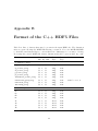
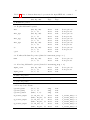
4.6 Format of the HDF5 Input and Output files
4.7 Compiling the C++ Source Code in Linux .
ii
.
.
.
.
.
.
.
.
.
.
.
.
.
.
.
.
.
.
.
.
.
.
.
.
.
.
.
.
.
.
.
.
.
.
.
.
.
.
.
.
.
.
.
.
.
.
.
.
.
.
.
.
.
.
.
.
.
.
.
.
.
.
.
.
.
.
.
.
.
.
.
.
.
.
.
.
.
.
.
.
.
.
.
.
.
.
.
.
.
.
.
.
.
.
.
.
.
.
.
.
.
.
.
.
.
.
.
.
.
.
.
.
.
.
.
.
.
.
.
.
.
.
.
.
.
CONTENTS
4.8
4.9
iii
Compiling the C++ Source Code in Windows . . . . . . . . . . . . . . . . . 59
Performance and Memory Usage . . . . . . . . . . . . . . . . . . . . . . . . 59
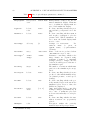
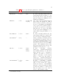
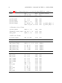
Appendix A List of Optional Input Parameters
61
Appendix B Format of the C++ HDF5 Files
64
Chapter 1
Introduction
1.1
Overview
k-Wave is an open source, third party, MATLAB toolbox designed for the time-domain
simulation of propagating acoustic waves in 1D, 2D, or 3D. The toolbox has a wide range
of functionality, but at its heart is an advanced numerical model that can account for both
linear and nonlinear wave propagation, an arbitrary distribution of heterogeneous material
parameters, and power law acoustic absorption [1, 2]. The interface to the simulation functions has been designed to be both flexible and user friendly, while the computational engine has been optimised for speed and accuracy. The functions are called using MATLAB
scripts with user-defined input parameters, so some familiarity with the MATLAB environment is necessary to get started. However, the toolbox now includes around 50 worked
examples and is also supported by an online forum (http://www.k-wave.org/forum).
k-Wave is still under active development, and its functionality is still evolving. This process is helped immensely by feedback from you, the user community. So if something is
missing, doesn’t work the way it should, or fails to do what you’d hoped, please get in
touch.
1.2
History and Contributors
The k-Wave toolbox was originally developed within the Photoacoustic Imaging Group at
University College London. The first beta version, released in July 2009, focussed primarily
on forward and inverse initial value problems for the simulation and reconstruction of
photoacoustic1 wave fields in lossless media [1]. Subsequent releases of the toolbox have
extended this functionality to include time varying pressure and velocity sources, acoustic
absorption, nonlinearity, and models for ultrasound transducers. The overall development
of the toolbox has been driven by Bradley Treeby and Ben Cox, while the C++ version of
kspaceFirstOrder3D was developed by Jiri Jaros. The work has been done at Australian
National University and University College London. A considerable number of other users,
1
Photoacoustic tomography is a biomedical imaging modality based on the thermoelastic generation of
ultrasound waves using pulsed laser light [3].
1
2
CHAPTER 1. INTRODUCTION
collaborators, and students have also contributed to this project, both directly (through
code development) and indirectly (through suggestions, usage feedback, and bug reports).
A sincere thanks goes to the user community for continuing to support the toolbox.
1.3
What’s in this Manual
This manual includes a general introduction to the governing equations and numerical
methods used in the main simulation functions in k-Wave. It also provides a basic overview
of the software architecture and a number of canonical examples. The content is divided
into three main sections, which can be read largely independently. Section 2 describes the
underlying governing equations and numerical methods, Sec. 3 describes how to use the
main simulation functions in MATLAB, and Sec. 4 describes how to install and use the
C++ code.
The manual is intended to accompany the extensive html documentation that is also
provided with the toolbox. After installation, the html documentation can be accessed
from the MATLAB help browser by selecting “k-Wave Toolbox” from the contents page.
In versions of MATLAB prior to 2012b, the help browser is opened by clicking on the
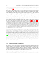
blue question mark icon
on the menu bar. In MATLAB 2012b (and later), the documentation is accessed by selecting “Help” from the ribbon bar, and then clicking on
“Supplemental Software”. This additional documentation provides detailed information
on how to use individual functions as well as around 50 worked examples.
1.4
Installation
The k-Wave toolbox is installed by adding the root k-Wave folder to the MATLAB path.
This can be done using the “Set Path” dialog box which is accessed by typing >> pathtool
at the MATLAB command line.2 This dialog box can also be accessed using the dropdown
menus “File → Set Path” if using MATLAB 2012a and earlier, or the the “Set Path”
button on the ribbon bar if using MATLAB 2012b and later. Once the dialog box is open,
the toolbox is installed by clicking “Add Folder”, selecting the k-Wave toolbox folder, and
clicking “save”. The toolbox can be uninstalled in the same fashion.
For Linux users, using the “Set Path” dialog box requires write access to pathdef.m. This
file can be found under <...matlabroot...>/toolbox/local. To find where MATLAB
is installed, type >> matlabroot at the MATLAB command line.
Alternatively, the toolbox can be installed by adding the line
addpath(‘<...pathname...>/k-Wave Toolbox’);
to the startup.m file, where <...pathname...> is replaced with the location of the toolbox, and the slashes should be in the direction native to your operating system. If no
startup.m file exists, create one, and save it in the MATLAB startup directory.
2
The >> symbol is the default MATLAB command prompt and is used here to denote commands that
are entered in the MATLAB command window. The symbol itself is not actually entered.
1.5. LICENSE
3
After installation, restart MATLAB. You should then be able to see the k-Wave help files
in the MATLAB help browser. Try selecting one of the examples and then clicking “run
the file”. If you can’t see “k-Wave Toolbox” in the contents list of the MATLAB help
browser, try typing >> help k-Wave at the command prompt to see if the toolbox has
been installed correctly. If it has and you still can’t see the help files, open “Preferences”
and select “Help” and make sure “k-Wave Toolbox” or “All Products” is checked.
After installation, to make the k-Wave documentation searchable from within the MATLAB help browser, run
>> builddocsearchdb(‘<...pathname...>/k-Wave Toolbox/helpfiles’);
again using the slash direction native to your operating system. Note, the created database
file will only work with the version of MATLAB used to create it.
If using the C++ version of kspaceFirstOrder3D (see discussion in Chapter 4), the appropriate binaries (and library files if using Windows) should also be downloaded from
http://www.k-wave.org/download.php and placed in the root “binaries” folder of the
toolbox.
1.5
License
c 2009-2012 Bradley Treeby, Ben Cox, and Jiri Jaros.
k-Wave The k-Wave toolbox is distributed by the copyright owners under the terms of the GNU
Lesser General Public License (LGPL). This is a set of additional permissions added
to the GNU General Public License (GPL). The full text of both licenses is included
with the toolbox in the folder “license” or is available online from http://www.gnu.org/
licenses/.
The LGPL license places copyleft restrictions on the k-Wave toolbox. Essentially, anyone
can use the software for any purpose (commercial or non-commercial), the source code
for the toolbox is freely available, and anyone can redistribute the software (in its original
form or modified) as long as the distributed product comes with the full source code and
is also licensed under the LGPL. You can make private modified versions of the toolbox
without any obligation to divulge the modifications so long as the modified software is not
distributed to anyone else. The copyleft restrictions only apply directly to the toolbox,
but not to other (non-derivative) software that simply links to or uses the toolbox.
k-Wave is distributed in the hope that it will be useful, but WITHOUT ANY WARRANTY; without even the implied warranty of MERCHANTABILITY or FITNESS FOR
A PARTICULAR PURPOSE. See the GNU Lesser General Public License for more details.
If you find the toolbox useful for your academic work, please consider citing:
B. E. Treeby and B. T. Cox, “k-Wave: MATLAB toolbox for the simulation
and reconstruction of photoacoustic wave-fields,” Journal of Biomedical Optics,
vol. 15, no. 2, p. 021314, 2010.
4
CHAPTER 1. INTRODUCTION
and/or:
B. E. Treeby, J. Jaros, A. P. Rendell, and B. T. Cox, “Modeling nonlinear
ultrasound propagation in heterogeneous media with power law absorption
using a k-space pseudospectral method,” Journal of the Acoustical Society of
America, vol. 131, no. 6, pp. 4324-4336, 2012.
The first paper gives an overview of the toolbox with applications in photoacoustics, and
the second describes the nonlinear ultrasound model and the C++ code.
1.6
Alternative Software
The k-Wave toolbox is a powerful tool for general acoustic modelling. However, this
doesn’t mean it’s the best tool for every purpose! There is a diverse range of other software
packages available that might be more appropriate in particular circumstances. We try to
maintain a list of useful acoustic packages at http://www.k-wave.org/acousticsoftware.
php. If you think we’ve made any errors or omissions, please get in touch.
Chapter 2
Numerical Model
2.1
Governing Equations
When an acoustic wave passes through a compressible medium, there are dynamic fluctuations in the pressure, density, temperature, particle velocity, etc. These changes can be
described by a series of coupled first-order partial differential equations based on the conservation of mass, momentum, and energy within the medium. Often in acoustics, these
equations are combined together into a single “wave equation” which is a second-order
partial differential equation in a single acoustic variable (most often the acoustic pressure). For example, in the classical case of a small amplitude acoustic wave propagating
through a homogeneous and lossless fluid medium, the first-order equations are given by
[4]
∂u
1
= − ∇p ,
∂t
ρ0
∂ρ
= −ρ0 ∇ · u ,
∂t
(momentum conservation)
(mass conservation)
p = c20 ρ .
(pressure-density relation)
(2.1)
Here u is the acoustic particle velocity, p is the acoustic pressure, ρ is the acoustic density, ρ0 is ambient (or equilibrium) density, and c0 is the isentropic sound speed. These
equations assume the background medium is quiescent (meaning there is no net flow and
the other ambient parameters don’t change with time) and isotropic (meaning the material parameters do not depend on the direction the wave is travelling). When they are
combined together, they give the familiar second-order wave equation
∇2 p −
1 ∂2p
=0 .
c20 ∂t2
(2.2)
The main simulation functions in k-Wave (kspaceFirstOrder1D, kspaceFirstOrder2D,
kspaceFirstOrder3D) solve the coupled first-order system of equations rather than the
equivalent second-order equation. This is done for several reasons. First, it allows both
mass and force sources to be easily included into the discrete equations. Second, it allows
5
6
CHAPTER 2. NUMERICAL MODEL
the values for the pressure and particle velocity to be computed on staggered grids which
improves numerical accuracy. Third, it allows the use of a special anisotropic layer (known
as a perfectly matched layer or PML) for absorbing the acoustic waves when they reach the
edges of the computational domain. Finally, the calculation of the particle velocity allows
quantities such as the acoustic intensity to be calculated. This is useful, for example, when
modelling how ultrasound heats biological tissue due to acoustic absorption.
The complexity of the governing equations used in k-Wave depends on the properties of the
simulation set by the user. Often, the acoustic medium is heterogeneous, with a spatially
varying sound speed and ambient density. In this case, the governing equations must
include some additional terms. Similarly, as an acoustic wave propagates, it generally loses
some acoustic energy to random thermal motion resulting in acoustic absorption. When
the absorption parameters are defined (medium.alpha_coeff and medium.alpha_power),
k-Wave treats the medium as a sound-absorbing fluid in which the absorption follows a
frequency power law of the form
α = α0 ω y ,
(2.3)
where α is the absorption coefficient in units of Np m−1 , α0 is the power law prefactor in
Np (rad/s)−y m−1 , and y is the power law exponent. Absorption of this form is observed
in a number of different materials including marine sediments and biological tissue [5, 6].
This type of absorption model is accurate for situations in which the shear modulus is
negligible, such as is often the case in soft biological tissue.
When acoustic absorption and heterogeneities in the material parameters are included,
the system of coupled first-order partial differential equations becomes [7, 8]
∂u
1
= − ∇p ,
∂t
ρ0
∂ρ
= −ρ0 ∇ · u − u · ∇ρ0 ,
∂t
p = c20 (ρ + d · ∇ρ0 − Lρ) ,
(momentum conservation)
(mass conservation)
(pressure-density relation)
(2.4)
where d is the acoustic particle displacement. If the mass conservation equation and
the pressure-density relation are solved together, the additional ∇ρ0 terms cancel each
other, so they are not included in the discrete equations solved in k-Wave to improve
computational efficiency.
The operator L in the pressure-density relation is a linear integro-differential operator
that accounts for acoustic absorption and dispersion that follows a frequency power law.
The presence of acoustic absorption must physically be accompanied by dispersion (a
dependence of the sound speed on frequency) to obey causality [9]. The operator used in kWave has two terms both dependent on a fractional Laplacian and is given by [10, 11]
L=τ
y −1
y+1 −1
∂
−∇2 2 + η −∇2 2
.
∂t
(2.5)
Here τ and η are absorption and dispersion proportionality coefficients
τ = −2α0 cy−1
0 ,
η = 2α0 cy0 tan (πy/2) ,
(2.6)
2.2. ACOUSTIC SOURCE TERMS
7
where α0 is the power law prefactor in Np (rad/s)−y m−1 , and y is the power law exponent.
The two terms in L separately account for power law absorption and dispersion for 0 <
y < 3 and y 6= 1 under particular smallness conditions [11]. These conditions are generally
satisfied for the range of attenuation parameters observed in soft biological tissue (for very
high values of absorption and frequency the behaviour of the loss operator deviates from
a power law due to second-order effects [12]).
In many situations in biomedical ultrasonics, the magnitude of the acoustic waves is high
enough that the wave propagation is no longer linear. In this case, additional nonlinear
terms also need to be included in the governing equations [13]. k-Wave doesn’t model all
the possible nonlinear effects that might occur in a fluid; it is not a computational fluid
dynamics (CFD) solver. Instead, it currently includes two additional nonlinear terms that
account for cumulative nonlinear effects to second-order in the acoustic variables. This is
an accurate model for many situations in biomedical ultrasound. When the nonlinearity
parameter medium.BonA is defined by the user, the system of coupled first-order equations
solved by k-Wave becomes [2, 14]
∂u
1
= − ∇p ,
∂t
ρ0
∂ρ
= − (2ρ + ρ0 ) ∇ · u − u · ∇ρ0 ,
∂t
B ρ2
2
p = c0 ρ + d · ∇ρ0 +
− Lρ .
2A ρ0
(momentum conservation)
(mass conservation)
(pressure-density relation)
(2.7)
Here B/A is the nonlinearity parameter which characterises the relative contribution of
finite-amplitude effects to the sound speed [15]. Compared to the linear case, the mass
conservation equation includes an additional term which accounts for a convective nonlinearity in which the particle velocity contributes to the wave velocity [16]. The additional
term is written as a spatial (rather than temporal) gradient to make it efficient to numerically encode [2]. The four terms within the bracket in the pressure-density relation
separately account for linear wave propagation, heterogeneities in the ambient density,
material nonlinearity, and power law absorption and dispersion (the sound speed c0 and
the nonlinearity parameter B/A can also be heterogeneous). Again, the additional ∇ρ0
terms cancel each other when these equations are solved together, so they are not included
in the discrete equations solved in k-Wave. If the three coupled equations are combined,
they give a generalised form of the Westervelt equation [14, 17, 18].
2.2
Acoustic Source Terms
The equations given in the previous section describe how acoustic waves propagate under
various conditions, but they don’t describe how these waves are generated or added to the
medium. Theoretically, linear sources could be realised by adding a source term to any of
the equations of mass, momentum, or energy conservation [19]. (There are also nonlinear
acoustics sources, such as the emission of sound by turbulence, but these aren’t considered here). For example, adding a source term to the momentum and mass conservation
8
CHAPTER 2. NUMERICAL MODEL
equations describing linear wave propagation in a homogeneous medium gives
1
∂u
= − ∇p + SF ,
∂t
ρ0
∂ρ
= −ρ0 ∇ · u + SM ,
∂t
p = c20 ρ .
(momentum conservation)
(mass conservation)
(pressure-density relation)
(2.8)
Here SF is a force source term and represents the input of body forces per unit mass in
units of N kg−1 or m s−2 . SM is a mass source term and represents the time rate of the
input of mass per unit volume in units of kg m−3 s−1 (the term SM /ρ0 in units of s−1 is
sometimes called the volume velocity). In the corresponding second-order wave equation,
the source terms appear as
∇2 p −
1 ∂2p
∂
= ρ0 ∇ · SF − SM .
2
2
∂t
c0 ∂t
(2.9)
This illustrates that it is actually the spatial gradient of the applied force, and the time
rate of change of the rate of mass injection (volumetric acceleration) that give rise to sound
[20].
Classical examples of mass or volume velocity sources are vibrating pistons and radially
oscillating spheres (in general, bodies whose volume is oscillating). An example of a force
source is a sideways oscillating rigid object, such as a wire or rigid sphere. The primary
difference between mass and force sources is the directivity of the generated sound fields.
As force is a vector, a force source has an inherent direction associated with it. A point
force source acting in one-direction will thus produce a dipole field. In contrast, a pressure
source will radiate in all directions (although it’s possible for the shape of a pressure
transducer to focus the field more strongly in one direction than another). A point mass
source will thus produce a monopole field. Within k-Wave, force and mass sources are
applied as velocity and pressure (or density) sources, respectively.
It’s also possible to define a source term SH associated with the energy conservation
equation [19]. This corresponds to the injection of heat per unit volume per unit time,
for example, due to the absorption of energy from a modulated laser beam. If the rate of
heat input is sufficiently rapid that thermal diffusion can be neglected, heat sources can
be treated as mass sources, where
SM = SH β/Cp .
(2.10)
Here, β is the volume thermal expansivity in units of K−1 , and Cp is the constant pressure
specific heat capacity in J kg−1 K−1 . In the case of photoacoustic tomography, the heating
pulse typically occurs on a timescale much shorter than the characteristic acoustic travel
time (a condition called stress confinement), and so the source can also be modelled as an
initial value problem for the acoustic pressure [21].
2.3
Overview of the k-space pseudospectral method
There are a wide variety of different numerical methods available for the solution of partial differential equations. There are an even greater variety if you consider the different
2.3. OVERVIEW OF THE K-SPACE PSEUDOSPECTRAL METHOD
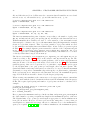
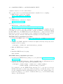
9
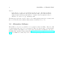
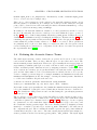
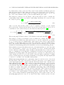
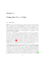
(a)
(b)
(c)
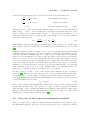
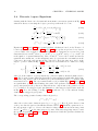
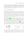
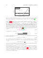
Figure 2.1: Calculation of spatial gradients using local and global methods. (a) Firstorder accurate forward difference. (b) Fourth-order accurate central difference. (c) Fourier
collocation spectral method.
possible permutations for each method. The “best” approach for discretising a particular
problem depends on many factors. For example, the size of the computational domain,
the number of frequencies of interest, the properties of the medium, the types of boundary
conditions, and so on. Here, we are interested in the time domain solution of the wave
equation for broadband acoustic waves in heterogeneous media. The drawback with classical finite difference and finite element approaches for solving this type of problem is that
at least 10 grid points per acoustic wavelength are generally required to achieve a useful
level of accuracy (a level of accuracy on a par with the uncertainty in the user-defined
inputs). This often results in computational grids that are simply to big to solve using
normal computers. To take an example, a diagnostic ultrasound image formed using a 3
MHz curvilinear transducer has a depth penetration around 15 cm. This distance is on
the order of 300 acoustic wavelengths at the fundamental frequency, and 600 wavelengths
at the second harmonic. If the acoustic parameters need to be discretised using 10 grid
points per wavelength, this translates into a 3D computational domain with more than
1011 grid elements. Even storing one matrix of this size in single-precision requires more
than 400 GB of computer memory! This problem is confounded further by the requirement
for small time steps to keep the simulation stable and to minimise unwanted numerical
errors.
To reduce the memory and number of time steps required for accurate simulations, k-Wave
solves the system of coupled acoustic equations described in the previous sections using
the k-space pseudospectral method (or k-space method) [22, 23, 24, 25]. This combines
10
CHAPTER 2. NUMERICAL MODEL
the spectral calculation of spatial derivatives (in this case using the Fourier collocation
method) with a temporal propagator expressed in the spatial frequency domain or k-space.
In a standard finite difference scheme, spatial gradients are computed locally based on the
function values at neighbouring grid points. In the simplest case, the gradient of the field
can be estimated using linear interpolation (see Fig. 2.1). A better estimate of the gradient
can be obtained by fitting a higher-order polynomial to a greater number of grid points
and calculating the derivative of the polynomial [26]. The more points used, the higher
the degree of polynomial required, and the more accurate the estimate of the derivative.
The Fourier collocation spectral method takes this idea further and fits a Fourier series
to all of the data [27]. It is therefore sometimes referred to as a global, rather than
local, method. There are two significant advantages to using Fourier series. First, the
amplitudes of the Fourier components can be calculated efficiently using the fast Fourier
transform (FFT). Second, the basis functions are sinusoidal, so only two grid points (or
nodes) per wavelength are theoretically required, rather than the six to ten required in
other methods.
While the Fourier collocation spectral method improves efficiency in the spatial domain,
conventional finite difference schemes are still needed to calculate the gradients in the time
domain. For example, using the second-order wave equation for homogeneous and lossless
media
1 ∂2
∇2 p (x, t) − 2 2 p (x, t) = 0 ,
(2.11)
c0 ∂t
a simple pseudospectral solution can be derived by taking the spatial Fourier transform and
then discretising the time derivative using a second-order accurate central difference1
p (k, t + ∆t) − 2p (k, t) + p (k, t − ∆t)
= − (c0 k)2 p (k, t) .
(2.12)
∆t2
Here k 2 = k · k = kx2 + ky2 + kz2 , where k is the wavevector, ∆t is the spacing between time
points, and we have used the relationship for the Fourier transform of the derivative of a
bounded function
Z
∂
1
F
f (x) = −
f (x)(−ikx )e−ikx x dx = ikx F {f (x)} ,
(2.13)
∂x
2π
where F is the spatial Fourier transform. Unfortunately, the finite difference approximation
of the temporal derivative introduces errors into the numerical solution that can only be
controlled by limiting the size of the time-step. The techniques broadly classed as k-space
methods attempt to relax this limitation in order to allow larger time-steps to be used
without compromising accuracy. Using an exact solution to the homogeneous and lossless
wave equation valid for an initial pressure distribution [25, 21, 12]
p (k, t) = cos (c0 kt) p (k, 0) ,
(2.14)
an exact pseudospectral scheme for Eq. (2.11) can be derived by substituting Eq. (2.14)
into the leapfrog finite difference p (k, t + ∆t) − 2p (k, t) + p (k, t − ∆t). After some rearrangement, this yields the relationship [25]
p (k, t + ∆t) − 2p (k, t) + p (k, t − ∆t)
= − (c0 k)2 p (k, t) .
2
2
∆t sinc (c0 k∆t/2)
1
(2.15)
This is the general approach for Fourier pseudospectral and k-space methods; by taking the spatial
Fourier transform of the equations, time dependent partial differential equations are reduced to ordinary
differential equations that can be integrated forward in time using implicit or explicit methods.
2.3. OVERVIEW OF THE K-SPACE PSEUDOSPECTRAL METHOD
11
By comparing the two pseudospectral schemes, we can see that the ∆t2 term in Eq. (2.12)
has been replaced with ∆t2 sinc2 (c0 k∆t/2) in Eq. (2.15). For small ∆t, these are approximately the same. However, for larger time steps, the additional sinc term provides
an exact solution, free from numerical dispersion. By extension, an exact pseudospectral
scheme for solving the acoustic equations expressed as coupled first-order partial differential equations can be obtained by replacing ∆t in a first-order accurate forward difference
with ∆t sinc (c0 k∆t/2) [25, 28]. The operator
κ = sinc (cref k∆t/2) ,
(2.16)
is known as the k-space operator, where cref is a scalar reference sound speed.
For large-scale acoustic simulations where the waves propagate over distances of hundreds
or thousands of wavelengths, this seemingly small correction becomes critically important.
Without this term, the finite difference approximation of the temporal derivative introduces phase errors which accumulate as the simulation runs. For small simulations, this
accumulation is generally not a problem. However, to retain the same level of accuracy
as the size of the simulation is increased, the size of the time steps must be continually
reduced. This can significantly increase compute times, particularly in comparison to the
k-space method which remains dispersion free, regardless of the simulation size. When
nonlinearity, heterogeneous material parameters, or acoustic absorption are included in the
governing equations, the temporal discretisation using the k-space operator is no longer
exact. However, if these perturbations are small, the inclusion of this operator can still
significantly reduce the unwanted numerical dispersion [24, 25, 2].
As well as the use of the k-space operator, additional accuracy and stability can also be obtained when computing odd-order derivatives by using staggered spatial and temporal grids
[29]. For the Fourier collocation spectral method, spatial shifts can be easily obtained using
the shift property of the Fourier transform, where Fx {f (x + ∆x)} = eikx ∆x Fx {f (x)}. Details of the staggered grid scheme used in k-Wave are given in the following section.
Rather than using a Fourier basis to calculate the spatial gradients, it is also possible to use
an alternative form of the pseudospectral method that uses Chebyshev polynomials [30].
There are several reasons why the Fourier method, rather than the Chebyshev method,
is used in k-Wave. First, it is straightforward to calculate the k-space operator when the
gradients are computed using a Fourier basis, giving improved accuracy for large time
steps as mentioned above. Second, when using Chebyshev polynomials, the grid points
must be clustered closer together near the boundaries to avoid the Runge phenomenon
[30, 31]. This means for the same maximum frequency, more grid points are needed.
For example, a common choice is cosine-spaced points [31]. Compared to the Fourier
method, this would require (π/2)N more grid points for an N -dimensional simulation.
For 3D simulations, this increases the memory consumption by almost four times. Third
(although perhaps less importantly), using a Fourier basis is more intuitive to acousticians
who often think in the wavenumber-frequency domain. The main argument in favour of
using Chebyshev polynomials is that they do not make the assumption of periodicity, and
are therefore compatible with a range of boundary conditions. However, for simulations in
infinite domains, it is straightforward to counteract the periodicity assumed by the Fourier
method using a perfectly matched layer (see discussion in Sec. 2.6).
12
2.4
CHAPTER 2. NUMERICAL MODEL
Discrete k-space Equations
Starting with the linear case, the mass and momentum conservation equations in Eq. (2.4)
written in discrete form using the k-space pseudospectral method become
n
n oo
∂ n
p = F−1 ikξ κ eikξ ∆ξ/2 F pn
,
∂ξ
1
1
n+
n−
∆t ∂ n
uξ 2 = uξ 2 −
p + ∆t SnFξ ,
ρ0 ∂ξ
1 n+ 2
∂ n+ 12
−ikξ ∆ξ/2
−1
ikξ κ e
F uξ
u
=F
,
∂ξ ξ
ρn+1
= ρnξ − ∆tρ0
ξ
∂ n+ 12
n+ 1
+ ∆t SMξ 2 .
uξ
∂ξ
(2.17a)
(2.17b)
(2.17c)
(2.17d)
Equations (2.17a) and (2.17c) are spatial gradient calculations based on the Fourier collocation spectral method, while (2.17b) and (2.17d) are update steps based on a k-space
corrected first-order accurate forward difference. These equations are repeated for each
Cartesian direction in RN where ξ = x in R1 , ξ = x, y in R2 , and ξ = x, y, z in R3 (N
is the number of spatial dimensions). Here, F and F−1 denote the forward and inverse
spatial Fourier transform, i is the imaginary unit, kξ represents the wavenumbers in the
ξ direction, ∆ξ is the grid spacing in the ξ direction, ∆t is the time step, and κ is the
k-space operator defined in Eq. (2.16). The discrete wavenumbers are defined according
to

h
i
Nξ
Nξ
Nξ
2π

−
,
−
+
1,
.
.
.
,
−
1

2
2
2
∆ξ Nξ if Nξ is even

kξ =
(2.17e)
h
i


(N
−1)
(N
−1)
(N
−1)
ξ
ξ
ξ
2π
 −
,−
+ 1, . . . ,
if Nξ is odd
2
2
2
∆ξ Nξ
where Nξ is the number of grid points in the ξ direction (this is discussed further in Sec.
3.2). The acoustic density (which is physically a scalar quantity) is artificially divided into
Cartesian components to allow an anisotropic perfectly matched layer to be applied (this
is discussed in Sec. 2.6). The exponential terms e±ikξ ∆ξ/2 within Eqs. (2.17a) and (2.17c)
are spatial shift operators that translate the result of the gradient calculations by half the
grid point spacing in the ξ-direction. This allows the components of the particle velocity
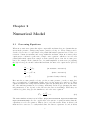
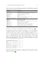
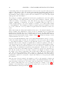
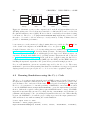
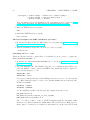
to be evaluated on a staggered grid. An illustration of the staggered grid scheme is shown
in Fig. 2.2. Note, the density ρ0 in Eq. (2.17b) is understood to be the ambient density
defined at the staggered grid points.
The corresponding pressure-density relation is given by
pn+1 = c20 ρn+1 − Ld
,
(2.17f)
P
where the total acoustic density is given by ρn+1 = ξ ρn+1
. Here Ld is the discrete form
ξ
of the power law absorption term which is discussed in Sec. 2.5. In all the equations above,
the superscripts n and n + 1 denote the function values at current and next time points
and n − 12 and n + 12 at the time staggered points. This time-staggering arises because
the update steps, Eqs. (2.17b) and (2.17d), are interleaved with the gradient calculations,
Eqs. (2.17a) and (2.17c).
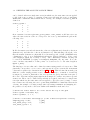
2.4. DISCRETE K-SPACE EQUATIONS
13
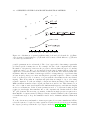
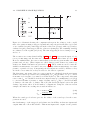
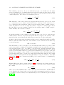
Figure 2.2: Schematic showing the computational steps in the solution of the coupled
first-order equations using a staggered spatial and temporal grid in 2D. Here ∂p/∂x and
ux are evaluated at grid points staggered in the x-direction (crosses), while ∂p/∂y and uy
evaluated at grid points staggered in the y-direction (triangles). The remaining variables
are evaluated on the regular grid (dots). The time staggering is denoted using n, n + 12 ,
and n + 1.
The acoustic source terms defined in Eqs. (2.17b) and (2.17d) represent the input of body
forces per unit mass, and the time rate of input of mass per unit volume (see Sec. 2.2).
However, within k-Wave, the source terms defined by the user are given in units of acoustic
pressure and velocity. (These inputs are called source.p and source.ux, source.uy,
source.uz. Further discussion is given in Sec. 3.4). These terms are used because the
available measurements of acoustic sources are typically either measurements of acoustic
pressure or particle velocity. Consequently, the user inputs are scaled by k-Wave so they
are in the correct units before they are added to the discrete equations.
The Cartesian components of the force source term SFξ are calculated from the user inputs
source.ux, source.uy, source.uz by multiplying by c0 /∆ξ (in units of s−1 ) to convert
from units of velocity (m s−1 ) to units of acceleration (m s−2 ). The components of the mass
source term SMξ are calculated from the user input source.p by multiplying by 1/(N c20 )
to convert from units of pressure to units of density, and by c0 /∆ξ to convert from units
of density to the time rate of density. The 1/N term divides the input between the split
density components, where N is the number of dimensions. Using the x-direction as an
example, the final source scaling factors used in k-Wave are
2c0
,
∆x
source.p 2c0
=
.
∆x
c20 N
SFx = source.ux
(2.18)
SMx
(2.19)
When the sound speed is heterogeneous, the values of the sound speed at the source
positions are used.
One disadvantage of the staggered grid scheme used in k-Wave is that user inputs and
outputs must also follow this scheme. This means inputs and outputs for the particle
14
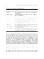
CHAPTER 2. NUMERICAL MODEL
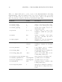
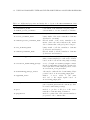
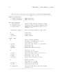
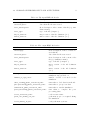
Table 2.1: Effect of the staggered grid scheme on the input and output pressure and
particle velocity values in 3D.
Parameter
Position
Time
x-direction velocity input
x-direction velocity output
y-direction velocity input
y-direction velocity output
z-direction velocity input
z-direction velocity output
x + ∆x/2, y, z
x + ∆x/2, y, z
x, y + ∆y/2, z
x, y + ∆y/2, z
x, y, z + ∆z/2
x, y, z + ∆z/2
t
t + ∆t/2
t
t + ∆t/2
t
t + ∆t/2
pressure input
pressure output
x, y, z
x, y, z
t + ∆t/2
t + ∆t
velocity are defined on staggered grid points, while inputs and outputs for the pressure
are defined on regular grid points. This is further complicated by the staggered time
scheme, as the outputs for both pressure and velocity are offset by ∆t/2 relative to the
inputs. However, with a little care, it is possible to compensate for these offsets. The effect
of the staggered grid scheme on the inputs and outputs is summarised in Table 2.1.
The time staggering also affects how the initial conditions are defined for an initial value
problem (IVP). For example, when modelling an IVP for the pressure for which the particle
velocity is zero at time t = 0 (this is the case in photoacoustic imaging), it is not possible
to directly impose u0ξ = 0. Instead, it is necessary to impose odd symmetry by setting
−1/2
1/2
uξ
= −uξ . This is done automatically within the simulation functions when the user
sets a value for source.p0 (a discussion of the source terms is given in Sec. 3.4).
Returning to the discrete equations, in the nonlinear case, the mass conservation equation
also includes a convective nonlinearity term, and thus Eq. (2.17d) becomes
1
n+ 2
=
ρn+1
ξ
∂
ρnξ − ∆tρ0 ∂ξ
uξ
1+
1
∂ n+ 2
2∆t ∂ξ
uξ
n+ 1
∆t SMξ 2
+
1+
1
∂ n+ 2
2∆t ∂ξ
uξ
.
(2.20)
The nonlinear correction to the mass source term arises because the temporal gradient in
the mass conversation equation from Eq. (2.7) is solved using an implicit finite difference
scheme (the acoustic density term on the right hand side is taken to be ρn+1 rather than
ρn ). Because the effect of the nonlinear term on the source is small, it is neglected in the
discrete equations implemented in k-Wave. The corresponding pressure-density relation
includes a material nonlinearity term and is given by
B 1 n+1 2
n+1
2
n+1
p
= c0 ρ
+
ρ
− Ld ,
(2.21)
2A ρ0
P
where the total acoustic density is again given by ρn+1 = ξ ρn+1
.
ξ
The calculation of first-order gradients using the Fourier collocation spectral method normally requires a Fourier transform over only one dimension. For example, to compute the
gradient in the x-direction, the Fourier transform is performed over the x-dimension, the
2.5. MODELLING POWER LAW ACOUSTIC ABSORPTION
15
result is multiplied by ikx (the wavenumbers in the x-direction), and the inverse Fourier
transform is then performed. A penalty of including the k-space operator κ in the discrete
equations is that the Fourier transform must be performed over RN rather than R1 . In
other words, for a 3D simulation, the Fourier transforms must be three dimensional. This
is because the k-space operator depends on the scalar wavenumber k, given by
q
√
k = k · k = kx2 + ky2 + kz2 ,
(2.22)
which varies in all three dimensions. The major advantage is that for homogeneous media, the inclusion of the k-space operator makes the temporal discretisation exact. This
means the time steps can be made arbitrarily large to compensate for this penalty. In
the heterogeneous case, for small simulations a rough rule of thumb is that the operator
allows the time steps to be three times larger for a similar level of accuracy (although this
is very problem dependent [25, 32, 2]). For most simulations, the calculation of Fourier
transforms accounts for about 60% of the total compute time [33]. Thus, even after accounting for the increase in time to calculate the Fourier transforms, the k-space approach
still reduces the overall compute time on the order of 50% in 2D, and 25% in 3D. The
advantage of the k-space method becomes more marked as the size of the simulation is
increased because of the accumulation of phase error (see discussion in Sec. 2.3).
2.5
Modelling Power Law Acoustic Absorption
The acoustic absorption in most biological tissues over the MHz frequency range has
been experimentally observed to follow a frequency power law [34]. As mentioned in Sec.
2.1, k-Wave uses an absorption term based on the fractional Laplacian to account for
this behaviour [10, 11]. Compared to absorption operators based on temporal fractional
derivatives [35, 36, 37, 38, 39, 40], the advantage of this form of the absorption term is
that it can be computed efficiently using Fourier spectral methods [11, 2]. The principal
alternative is to include a sum of relaxation absorption terms [41, 25]. However, this is more
memory intensive and requires the relaxation parameters to be obtained using a fitting
procedure for each value of absorption and range of frequencies under consideration.
Returning to the discretised equations, the spatial Fourier transform of the negative fractional Laplacian has the simple form [42, 10]
a F −∇2 ρ = k 2a F {ρ} ,
which allows the discrete form of the power law absorption term to be written as [11]
n ∂ρ
−1
y−2
−1
y−1
n+1
Ld = τ F
k
F
+ηF
k
F ρ
.
(2.23)
∂t
To avoid needing to explicitly calculate the time derivative of the acoustic density (which
would require storing a copy of at least ρn and ρn−1 in memory), the temporal derivative
of the acoustic density is replaced using the linearized mass conservation equation dρ/dt =
−ρ0 ∇ · u, which gives
X
∂ n+ 12
−1
y−1
n+1
−1
y−2
uξ
+ηF
k
F ρ
.
(2.24)
Ld = −τ F
k
F ρ0
ξ ∂ξ
16
CHAPTER 2. NUMERICAL MODEL
It is clear from the notation used here that the numerical values for the acoustic density and
particle velocity are temporally offset by dt/2. This introduces an additional phase offset
between the acoustic density and the pressure, which causes a small error in the modelled
values of absorption and dispersion (using a simple finite difference approximation to ∂ρ/∂t
also results in a similar phase error). For most simulations, the accuracy of the modelled
acoustic absorption and dispersion should be sufficient. If increased numerical precision is
required, the size of the time step can be reduced.
2.6
Perfectly Matched Layer
In Fourier pseudospectral and k-space numerical models, the use of the FFT to calculate
spatial gradients implies that the wave field is periodic. This causes waves leaving one
side of the domain to reappear at the opposite side. (In the 1D case, imagine a wave on
a closed loop of string; in 2D think of a wave propagating on the surface of a torus; in
3D it is harder to imagine!) Often we want to model the propagation of acoustic waves
in free space. This could be achieved by increasing the size of the computational grid so
that the waves never reach the boundaries. However, this approach carries a significant
computational penalty. Instead, we want the waves reaching the edge of the domain to
disappear, as if they were continuing off to infinity, rather than “wrapping round” and
re-appearing on the opposite side of the domain.
The wave wrapping caused by the FFT can be largely eliminated by the use a perfectly
matched layer (PML) [43, 44]. This is a thin absorbing layer that encloses the computational domain and is governed by a nonphysical set of equations that cause anisotropic absorption. In pseudospectral models there are two requirements that such a layer must meet:
(1) the layer must provide sufficient absorption so the outgoing waves are significantly attenuated, and (2) the layer must not reflect any waves back into the medium.
k-Wave uses Berenger’s original split-field formulation of the PML [43, 45]. This requires
the acoustic density or pressure to be artificially divided into Cartesian components, where
ρ = ρx + ρy + ρz . The absorption is then defined such that only components of the wave
field travelling within the PML and normal to the boundary are absorbed. Using the
homogeneous linear case to illustrate, the first-order coupled equations including the PML
become
∂uξ
1 ∂p
=−
− αξ uξ ,
∂t
ρ0 ∂ξ
∂ρξ
∂uξ
= −ρ0
− αξ ρ ξ ,
∂t
∂ξ
X
p = c20
ρξ .
(momentum conservation)
(2.25a)
(mass conservation)
(2.25b)
(pressure-density relation)
(2.25c)
ξ
Here α = {αx , αy , αz } is the anisotropic absorption in Nepers per second. All three
components are zero outside the PML, and inside the PML they are zero everywhere
except within a PML layer perpendicular to their associated direction. In other words,
for a PML perpendicular to the x-axis, α = {αx , 0, 0}. The fact that the absorption
coefficient is anisotropic in this way, and that the same absorption coefficient acts on both
2.6. PERFECTLY MATCHED LAYER
17
the density and particle velocity, is sufficient for there to be no reflections from the edge
of the PML (in the continuous homogeneous case).
Following [46, 25], Eqs. (2.25a) and (2.25b) are transformed using the relationship
∂
∂ αt +α f +Q=
e f + eαt Q ,
(2.26)
∂t
∂t
into the form
∂ αξ t
1 ∂p
(e uξ ) = −eαξ t
,
∂t
ρ0 ∂ξ
∂uξ
∂ αξ t
(e ρξ ) = −ρ0 eαξ t
.
∂t
∂ξ
Using first-order accurate forward differences to discretise the time derivatives, the discrete
equations given in Eq. (2.17b) and (2.17d) including a PML can then be written as
∆t ∂ n
n− 1
n+ 1
,
p
uξ 2 = e−αξ ∆t/2 e−αξ ∆t/2 uξ 2 −
ρ0 ∂ξ
∂ n+ 12
n+1
−αξ ∆t/2
−αξ ∆t/2 n
e
ρξ − ∆tρ0 uξ
ρξ = e
.
(2.27)
∂ξ
This is the form of the PML equations implemented in k-Wave.
So far, nothing has been said about the actual values of αξ . It would seem from the
equations above that large values should be used, as the waves will then be attenuated
quickly, and the required thickness of the PML minimised. However, the spatial discretisation must also be taken into account. Consider the case of a wave propagating in the
x direction. If αx is constant, between the edge of the PML and one grid point inside,
the wave will be forced to decrease by a factor of exp(−αx ∆x/c0 ). If αx is large then the
PML will impose a large gradient across the PML boundary, which will cause a reflection
of the incoming wave. One way to reduce this reflection is to set αx c0 /∆x. However,
then the decay within the PML will be slow, and a very thick PML will be required to
avoid significant wave wrapping. A better way is to make αξ a function of position within
the PML, where αξ = αξ (ξ), so that the shape of the decay can be changed to make it
smoother at the boundary edge. k-Wave uses the following function [25]
m
ξ − ξ0
αξ = αmax
,
(2.28)
ξmax − ξ0
where ξ0 is the coordinate at the start of the PML and ξmax is the coordinate at the
end. Following Tabei et al., [25] m = 4 is used to give a balance between minimising
the amplitude of the wrapped wave and minimising the amplitude of the reflected wave.
Using a staggered spatial grid makes a significant improvement to the performance of the
PML.
The PML absorption coefficient αξ used in the equations above is defined in units of Nepers
s−1 . Within k-Wave, the absorption parameter PML_alpha is instead defined in normalised
units of Nepers per grid point, where PML_alpha = (∆ξ/c0 )αξ . The corresponding PML
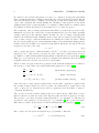
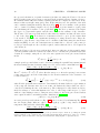
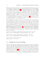
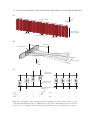
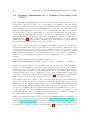
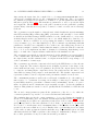
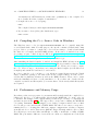
thickness PML_size is also defined in units of grid points. Figure 2.3 illustrates how the
PML transmission and reflection coefficients change with variations in PML_alpha and
PML_size. By default, k-Wave uses PML_alpha = 2 and PML_size = 20 for 1D and 2D
18
CHAPTER 2. NUMERICAL MODEL
0
Reflection [dB]
−20
−40
−60
−80
−100
0
10
PML Thickness
[grid points]
20
5
4
3
2
1
0
PML Absorption [Np/grid point]
0
Transmission [dB]
−20
−40
−60
−80
−100
0
10
PML Thickness
[grid points]
20
5
4
3
2
1
0
PML Absorption [Np/grid point]
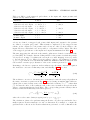
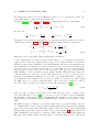
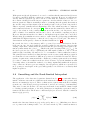
Figure 2.3: Performance of the split-field perfectly matched layer (PML) with variations
in the layer thickness and absorption coefficient.
simulations, and PML_alpha = 2 and PML_size = 10 for 3D simulations (the smaller size is
used to save grid real-estate). For PML_size = 10, the amplitude of the transmitted wave
is reduced by 84 dB, while the reflected coefficient is −65 dB. For PML_size = 20, the
transmission and reflection coefficients are improved to −100 dB and −80 dB, respectively.
This corresponds to around 4 or 5 decimal places of accuracy, which should be sufficient
for most simulations (see discussion in Sec. 3.8). It is possible to change the values for
PML_alpha and PML_size using the optional input parameters ‘PMLAlpha’ and ‘PMLSize’
(see discussion in Sec. 3.6). Note, the formulation of the PML and the default PML values
are based on the assumption of a homogeneous and lossless medium. For media with very
strong acoustic absorption, the efficacy of the PML is reduced.
2.7. ACCURACY, STABILITY AND THE CFL NUMBER
2.7
19
Accuracy, Stability and the CFL Number
In the previous sections, the continuous equations describing the propagation of linear and
nonlinear waves in heterogeneous and absorbing media, along with the discretisation of
these equations using the k-space pseudospectral method have been discussed. Here we
consider the question: when will the numerical model derived in Sec. 2.4 give the correct
solution to the continuous governing equations discussed in Sec. 2.1? There are three
aspects to this:
1. Are the discrete model equations equivalent to the continuous governing equations?
2. Is the numerical model stable?
3. Are the results it generates accurate?
The first question is asking whether the discrete equations are consistent or compatible
with the continuous equations. In other words, whether they become the continuous
equations in the limit as the spacing between the discrete spatial and temporal points
approaches zero, in the same way that the simple finite difference scheme (p(t + ∆t) −
p(t))/∆t → ∂p/∂t as ∆t → 0. In this case, the discrete equations given in Eq. (2.17)
are derived rigorously from the governing equations given in Eq. (2.4), and thus they are
consistent with them.
The second question is whether the numerical model based on these discrete equations is
stable or not. In other words, whether or not the numerical errors grow exponentially as
the model steps through time. It is important to note that some consistent schemes are
not stable. In other words, there are some numerical schemes derived directly from the
continuous equations, and equal to them in the limit, whose output will never be a good
approximation to the underlying system of partial differential equations.
Often, the stability or otherwise of a scheme depends on the size of the timestep, ∆t. The
stability condition for the discrete equations used in k-Wave can be derived straightforwardly in the case of a homogeneous, non-absorbing medium. In this case the discrete
equations given in Eq. (2.17) can be written in the simpler form
1
n+ 2
Ukξ
1
n− 2
= Ukξ
−
ikξ κ ∆t n
P ,
ρ0
1
n+ 2
P n+1 = P n − ikξ κ ∆tρ0 c20 Ukξ
(2.29a)
,
(2.29b)
where P n (k) = F {pn (x)} and Uknξ (k) = F{unξ (x)} are the pressure and particle velocity
variables in the spatial frequency or wavenumber domain. Writing the pressure at the
previous time step as
1
n− 2
P n = P n−1 − ikξ κ ∆tρ0 c20 Ukξ
,
(2.30)
subtracting Eq. (2.30) from Eq. (2.29b) and substituting in Eq. (2.29a) then gives
P n+1 − 2P n + P n−1 = −b2 P n ,
where b = kκ∆tc0 .
(2.31)
20
CHAPTER 2. NUMERICAL MODEL
3
Leapfrog PS
k−space
Phase Error [%]
2.5
2
1.5
1
0.5
0
sound speed range for
soft biological tissue
0
500
1000
1500
2000
Reference Sound Speed [m/s]
2500
3000
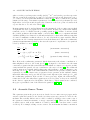
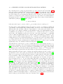
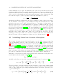
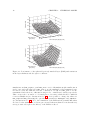
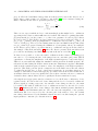
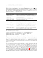
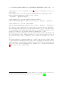
Figure 2.4: Phase error in the propagation of a plane wave after 50 wavelengths against
the reference sound speed cref used in the k-space operator κ for c0 = 1500 m/s [2].
Equation (2.31) is in the form of a simple difference equation, and the range of values of b
for which it generates a stable sequence . . . , P n−1 , P n , P n+1 , . . . can be found by assuming
the solution at timestep n has the form P n = (A)n B, where the n on A indicates a power
rather than a timestep index. A denotes the factor that is effectively multiplied to the old
P to obtain the new one at every timestep, hence the system is stable so long as |A| ≤ 1.
(This is consistent with our physical understanding of waves in homogeneous media; for
plane waves the amplitude will stay constant, while for all other waves the amplitude will
decay.) Substituting this equality into Eq. (2.31) leads to the characteristic quadratic
equation
A2 + (b2 − 2)A + 1 = 0 ,
(2.32)
for which the two solutions are
A1,2 =
−(b2 − 2) ±
p
(b2 − 2)2 − 4
.
2
(2.33)
It can be shown that |A| ≤ 1 when |b| ≤ 2. In other words, the numerical model used in
k-Wave is stable when
|kκ∆tc0 | ≤ 2 for all k .
(2.34)
For a pseudospectral time domain model κ = 1, so the stability criterion is simply
kmax ∆tc0 ≤ 2. For the k-space method κ = sinc (cref k∆t/2) and so the stability criterion
becomes
cref
.
(2.35)
|sin (cref k∆t/2)| ≤
c0
In a homogeneous medium the k-space method can be made unconditionally stable (and
exact) by choosing cref = c0 , as sine is never greater than 1.
It is interesting to note that if cref is chosen so that (cref /c0 ) > 1 then the model will also
be unconditionally stable, but the k-space operator κ will now no longer correct the phase
exactly, so phase errors will accumulate. As shown in Fig. 2.4, the larger cref /c0 is than
1, the greater the phase error will be, and it will grow until the solution is completely
corrupted. So with this choice of cref , the model is stable (the solution doesn’t “blow up”)
but it is not necessarily accurate.
2.7. ACCURACY, STABILITY AND THE CFL NUMBER
21
The remaining option is to choose cref such that (cref /c0 ) < 1. In this case, the phase
errors are guaranteed to be smaller than in the pseudospectral case (the k-space model
becomes the pseudospectral model as cref → 0 because κ → 1), but the model is now only
conditionally stable. The criterion for stability is given by
cref
2
∆t ≤
sin−1
.
(2.36)
cref kmax
c0
This discussion of the homogeneous case suggests that in the heterogeneous case, when
c0 = c0 (x), there are two options: (1) if the reference sound speed in κ is chosen to be
cref = max(c0 (x)) then stability is ensured but the timestep must be small enough to
ensure the phase error does not corrupt the solution, or (2) if cref = min(c0 (x)) is chosen
then the phase error is necessarily bounded but the timestep must be small enough to
ensure stability. The criterion for this is:
2
cref
−1
∆t ≤
.
(2.37)
sin
cref kmax
max(c0 )
A stability analysis for the nonlinear, absorbing model does not lead to such succinct
results as these. However, in general, absorption will act to improve the accuracy of the
numerical solution as it dampens the high frequencies introduced by the nonlinearity.
A number that is useful when discussing stability is the Courant-Friedrichs-Lewy (CFL)
number, which is defined as the ratio of the distance a wave can travel in one time step
to the grid spacing:
CFL ≡ c0 ∆t/∆x .
(2.38)
The CFL number could be thought of as a non-dimensionalised time step, and for that
reason it is useful for defining the maximum permissible time step without reference to
a specific grid spacing. Note, care must be exercised when comparing particular values
for the CFL stability condition between different types of numerical models (e.g., between
pseudospectral and finite difference models) as the CFL number is dependent on the grid
spacing. As an example, a value of CFL = 0.3 in a pseudospectral model with 2 grid points
per wavelength will equate to a time step 5 times larger than a finite difference model with
10 grid points per wavelength and the same CFL number. Using the definition of the CFL
number, Eq. (2.34) can be rewritten as |κ|CFL ≤ 2/π because kmax ∆x = π. Similarly Eq.
(2.36) then becomes
2 c0
−1 cref
CFL ≤
sin
.
(2.39)
π cref
c0
Within k-Wave, the discrete equations in Sec. 2.4 are iteratively solved using a time step
based on the CFL number given by the user. The size of the time step is calculated using
the formula
CFL∆x
∆t =
,
(2.40)
cmax
where cmax is the maximum value of the sound speed in the medium. A CFL number
of 0.3 (which is the default value used in the function makeTime) typically provides a
good balance between accuracy and computational speed for weakly heterogeneous media
[25, 32, 2].
22
CHAPTER 2. NUMERICAL MODEL
With questions (1) and (2) answered, we can be confident that the numerical model is stable and is compatible with the continuous governing equations. However, we still haven’t
directly answered question (3). How can we be sure that the results are accurate, i.e.,
the solution calculated from the discrete equations coincides with the solution to the continuous equations? This is essentially a matter of ensuring that the spatial discretisation
∆x and the temporal discretisation ∆t are small enough for the problem being studied.
This is expressed formally in Lax’s Equivalence Theorem, which says that a consistent,
stable numerical scheme is convergent [47]. This means the numerical solution will converge to the solution of the continuous equations as ∆t and ∆x → 0. In practice, there
will be a limit to how small ∆x and ∆t can be due to the available computing resources.
However, this just means there is a limit to the highest frequency that can be modelled.
When setting up a simulation it is necessary to ensure that the grid spacing is sufficiently
small that the highest frequency of interest can be supported by the grid. The issues of
discretisation and frequency content are discussed further in Sec. 3.4.
In general, the choice of the timestep will be governed by several considerations. In the
homogeneous case, the model will give accurate results for any timestep, but if a time
varying output that contains all the frequencies that the grid can support is required, the
timestep must satisfy ∆t ≤ ∆x/cmax , which is the same as saying CFL ≤ (c0 /cmax ). In
the heterogeneous case, ∆t (or equivalently the CFL number) must not only be chosen
small enough for stability, but may need to be even smaller to achieve sufficient accuracy.
The principal reason is that decreasing ∆t improves the accuracy with which propagation
across interfaces between media of different properties are dealt with. Because the discrete
system of equations is consistent with the continuous governing equations, there is a simple
procedure to ensure the results from the model are accurate: repeat the simulations with
decreasing values of ∆t until the results do not change significantly within the frequency
range of interest. In heterogeneous examples, lower frequencies, which are represented by
more points per wavelength on the grid, will typically be modelled more accurately than
higher frequencies.
2.8
Smoothing and the Band-Limited Interpolant
The application of the discretised equations discussed in Sec. 2.4 for particular discrete
initial conditions can result in oscillations in the numerical solution for the pressure field
that are not intuitively expected. These oscillations are a purely numerical effect resulting
from the use of the Fourier pseudospectral method, and are not evidence of an instability.
They arise because the Fourier collocation spectral method uses an FFT of finite length
to calculate spatial gradients, so the field parameters are implicitly represented using a
truncated Fourier series. The Fourier coefficients P (km ) are chosen so that the continuous
function p̂(x) given by
1
p̂(x) =
Nx
Nx /2−1
X
2πi mx
∆x
P (km )e− Nx
,
(2.41)
m=−Nx /2
matches the discretised function p(xj ) at the grid points x = xj . (Matching at a discrete
set of points is the defining feature of a collocation method.) The continuous function,
2.8. SMOOTHING AND THE BAND-LIMITED INTERPOLANT
23
p̂(x), is called the band-limited interpolant as it interpolates between the discrete set of
grid points xj using a finite set of Fourier components [48]. It is constructed using the
FFT coefficients at the discrete spatial frequencies km , where
Nx /2−1
P (km ) =
X
2πi
p(xj )e Nx mj .
(2.42)
j=−Nx /2
There are two aspects which are key to understanding how this might lead to oscillations
appearing in the solution, unless sufficient care is taken. The first is recognising that while
p̂(x) may match p(xj ) at the points x = xj , there is no guarantee about how p̂(x) behaves
in between these points. If there are large jumps in p(xj ) between adjacent points, i.e., if
p(xj ) − p(xj−1 ) is large, then p̂(x) might have to oscillate in between points xj−1 and xj in
order to reach p(xj ). The second is realising that it is the band-limited interpolant p̂ and
not p(xj ) that is propagated during the simulation. Consequently, when p̂ is resampled
at the discrete grid points xj at a later timestep, oscillations can appear in the solution.
An example of this is shown in Fig. 2.5, where the discrete pressure is shown with a stem
plot, and the underlying band limited interpolant is shown as a solid line [12].
If desired, it is possible to reduce the visible oscillations in the solution by making p(xj )
smoother, i.e., by reducing the size of the jumps between consecutive grid points. This is
equivalent to reducing the amplitudes of the higher spatial frequency components P (km ).
This is done automatically within the simulation functions when an initial pressure distribution is defined using the k-Wave function smooth. This function applies a Blackman
window in the spatial frequency domain to reduce the amplitude of the higher spatial frequencies. (The analogy in the purely continuous case is the link between the smoothness
of a function and the rate of decay of its Fourier transform. A very sharp function, for
example a delta function, has a flat frequency spectrum, whereas the Fourier transform of
an analytic function decays very quickly. In between these extremes, the more continuous
derivatives that a function has, the more quickly its Fourier transform decays.)
Selecting the most appropriate window or function to force the Fourier coefficients to decay
requires a trade off between the level of smoothing and the level of observable oscillations.
From a signal processing perspective, the amount of smoothing is related to the main
lobe width of the window, while the level of oscillations is related to the side lobe levels.
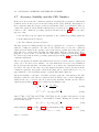
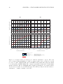
Figure 2.6 illustrates the effect of smoothing a delta function initial pressure distribution
using Hanning and Blackman windows. In both cases, the magnitude of the pressure
distribution has been corrected by the coherent gain of the window. Note, the default
smoothing behaviour used by the simulation functions can be modified using the optional
input parameter ‘smooth’ (see discussion in Sec. 3.6).
24
CHAPTER 2. NUMERICAL MODEL
p(x)
1
t=0
0.5
0
−10
p(x)
0.5
−5
0
x/ Δ x
5
10
−5
0
x/ Δ x
5
10
t = n Δt
0.25
0
−10
Figure 2.5: Propagation of an initial pressure distribution set to a discrete spatial delta
function. Oscillations appear in the solution at t = n∆t. The discrete pressure distribution
is shown with a stem plot, while the band-limited interpolant is shown with a solid line.
1
0.4
0.8
0.6
0.4
0.2
0.2
0.1
Hanning
Window
Relative Amplitude Spectrum
−0.1
1
0.5
0.4
0.8
Amplitude [au]
0.6
0.4
0.2
0.3
0.2
0.1
0
0
−0.1
Blackman
Window
1
Relative Amplitude Spectrum
Amplitude [au]
0.3
0
0
0.5
0.4
0.8
Amplitude [au]
Amplitude [au]
Frequency Response
0.5
Amplitude [au]
Amplitude [au]
Recorded Time Pulse
Relative Amplitude Spectrum
Spatial Source Shape
No Window
0.6
0.4
0.2
0.3
0.2
0.1
0
0
−0.1
0
5
10
x/ Δx
15
20
1
1.5
2
Time [μs]
2.5
3
1
0.8
0.6
0.4
0.2
1
0.8
0.6
0.4
0.2
1
0.8
0.6
0.4
0.2
0
0
5
10
15
Frequency [MHz]
20
Figure 2.6: Propagation of an initial pressure distribution set to a discrete delta function.
If no window is used, oscillations appear in the recorded pressure signal because of the
properties of the underlying band-limited interpolant. These oscillations can be reduced
by windowing the initial pressure distribution in the spatial frequency domain before the
simulation begins [12].
Chapter 3
First-Order Simulation
Functions
3.1
Overview
There are three simulation functions in the k-Wave Toolbox that implement the first-order
k-space model described in the previous chapter. These are named kspaceFirstOrder1D,
kspaceFirstOrder2D, and kspaceFirstOrder3D and correspond to simulating wave propagation in one, two, and three dimensions as their names imply. In this case, “first-order”
refers to the fact we are solving a system of coupled first-order partial differential equations. It’s not related to the order of numerical accuracy of the solution, or to the order
of the acoustic variables retained in the governing equations.
The simulation functions are called with four input structures; kgrid, medium, source,
and sensor. The properties of the simulation are then set as fields for these structures in
the form structure.field. The four structures respectively define the properties of the
computational grid, the material properties of the medium, the properties and locations of
any acoustic sources, and the properties and locations of the sensor points used to record
the evolution of the pressure and particle velocity fields over time. When the simulation
functions are called, the propagation of the wave-field in the medium is then computed
step by step, with the acoustic field at the sensor elements stored after each iteration.
These values are returned when the time loop has completed.
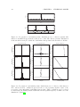
To illustrate the general structure of the MATLAB code required, a simple example of
using k-Wave to model an initial value problem in 2D is shown below. In this example,
the domain is divided into 128 by 256 grid points with a grid point spacing of 50 µm. The
sound speed is set to be heterogeneous, with a layer of higher speed near the top of the
domain. The source is set to be an initial pressure distribution in the shape of a disc, and
the sensor is set to be a circular array with 50 sensor points. The four input structures are
passed to kspaceFirstOrder2D which then calculates and returns the acoustic pressure
recorded at each sensor point for each time step.
During the simulation, a visualisation of the propagating wave-field and a status bar are
displayed, with frame updates every ten time steps. A snapshot of a 2D simulation of a
25
26
CHAPTER 3. FIRST-ORDER SIMULATION FUNCTIONS
focused ultrasound pulse is shown in Fig. 3.1(b). The k-Wave color map displays positive
pressures as yellows to reds to black, and negative pressures as light to dark blue-greys.
The default plot scale is set to display values from -1 to 1, with zero displayed as white.
Most of the default plot settings can be modified using optional input parameters as
described in Sec. 3.6.
% create the computational grid
Nx = 128;
% number of grid points
Ny = 256;
% number of grid points
dx = 50e-6;
% grid point spacing in
dy = 50e-6;
% grid point spacing in
kgrid = makeGrid(Nx, dx, Ny, dy);
in the x (row) direction
in the y (column) direction
the x direction [m]
the y direction [m]
% define the medium properties
medium.sound_speed = 1500*ones(Nx, Ny); % [m/s]
medium.sound_speed(1:50, :) = 1800;
% [m/s]
medium.density = 1040;
% [kg/m^3]
% define an initial pressure using makeDisc
disc_x_pos = 75;
% [grid points]
disc_y_pos = 120;
% [grid points]
disc_radius = 8;
% [grid points]
disc_mag = 3;
% [Pa]
source.p0 = disc_mag*makeDisc(Nx, Ny, disc_x_pos, disc_y_pos, disc_radius);
% define a Cartesian sensor mask of a centered circle with 50 sensor elements
sensor_radius = 2.5e-3;
% [m]
num_sensor_points = 50;
sensor.mask = makeCartCircle(sensor_radius, num_sensor_points);
% run the simulation
sensor_data = kspaceFirstOrder2D(kgrid, medium, source, sensor);
A detailed discussion of each of the four input structures is given in the following sections,
with a graphical view given in Fig. 3.1(a) for reference. There are also a large number of
worked examples included with the toolbox. These can be accessed through the MATLAB
documentation as described in Sec. 1.4.
3.2
Defining the Computational Grid
The first input kgrid defines the properties of the computational grid. This determines
how the continuous medium is divided up into a evenly distributed mesh of grid points
(the terms grid points and grid nodes are used here interchangeably). The grid points
represent the discrete positions in space at which the governing equations are solved. This
particular input must be created using the function makeGrid, which automatically creates
and populates the required fields. The syntax for creating a computational grid in 1D,
3.2. DEFINING THE COMPUTATIONAL GRID
27
(a)
kgrid
source
medium
sensor
c/ρ
.Nx
.dx
.t_array
.Nt
.dt
.k
.sound_speed
.density
.BonA
.alpha_power
.alpha_coeff
.p0
.p_mask
.p
.u_mask
.ux
.uy
.uz
.mask
.record
kspaceFirstOrder1D(kgrid, medium, source, sensor)
kspaceFirstOrder2D(kgrid, medium, source, sensor)
kspaceFirstOrder3D(kgrid, medium, source, sensor)
sensor_data
(b)
Figure 3.1: (a) Overview of the four inputs structures and the main input fields used
for the first-order simulation functions in k-Wave. (b) Snapshot of a 2D simulation of a
focused pulse using k-Wave. The source mask is shown as black line, and the progress
of the simulation is illustrated by the status bar. The anisotropic absorption within the
perfectly matched layer (PML) around the outside of the domain is also visible.
28
CHAPTER 3. FIRST-ORDER SIMULATION FUNCTIONS
2D, and 3D is shown below. k-Wave uses the convention that 1D variables are stored and
indexed as (x, 1), 2D variables as (x, y), and 3D variables as (x, y, z).
% create computational grid for a 1D simulation
kgrid = makeGrid(Nx, dx);
% create computational grid for a 2D simulation
kgrid = makeGrid(Nx, dx, Ny, dy);
% create computational grid for a 3D simulation
kgrid = makeGrid(Nx, dx, Ny, dy, Nz, dz);
The function makeGrid takes pairs of inputs corresponding to the number of grid points
(Nx, Ny, and Nz) and the grid point spacing (dx, dy, and dz) in each Cartesian direction.
Within makeGrid, these variables are used to create matrices of the wavenumbers and
Cartesian grid coordinates. An object of the kWaveGrid class (called kgrid in the examples
shown above) is then returned. This object has a number of properties which are used
by the simulation and utility functions within k-Wave. A list of these properties is given
in Table 3.1. For example, kgrid.x_size returns the total size of the computational grid
in the x-direction in metres, where kgrid.x_size = kgrid.Nx * kgrid.dx. An object
orientated approach for defining kgrid is used to enable many of the matrices to be created
on the fly, rather than being stored in memory.
The discrete wavenumber vectors kgrid.kx_vec, kgrid.ky_vec, and kgrid.kz_vec are
defined according to Eq. (2.17e) based on the values for Nx, Ny, Nz and dx, dy, dz. The
wavenumbers are used to calculate the spatial gradients of the acoustic field parameters
using the Fourier collocation spectral method as described in Sec. 2.4. The maximum
spatial frequency that can be represented by a particular computational grid is given
by the Nyquist limit of two grid points per wavelength, where kx_max = pi/dx. The
spatial wavenumber and temporal frequency are related by k = 2πf /c0 , thus the maximum
wavenumber corresponds to a maximum temporal frequency of f_max = min(c_0)/(2*dx).
If the grid spacing is not uniform in each Cartesian direction, the maximum frequency
supported in all directions will be dictated by the largest grid spacing.
When creating a new simulation, the easiest way to select appropriate values for Nx and dx
(etc) is to start with the desired domain size in metres and the maximum desired frequency
in Hz. The required grid spacing and number of grid points can then be calculated. For
example:
% compute dx and Nx based on a desired x_size and f_max
points_per_wavelength = 2;
dx = c0_min/(points_per_wavelength*f_max);
Nx = round(x_size/dx);
Here c0_min is the minimum sound speed in the medium, and points_per_wavelength is
the desired number of points per spatial wavelength at the maximum frequency of interest.
The Nyquist limit of two points per wavelength is appropriate for linear simulations in
homogeneous media. However, for heterogeneous media, using three or four points per
wavelength is recommended if accurate reflection coefficients close to the maximum frequency are required [24, 25, 32, 2]. For nonlinear simulations, the maximum frequency
3.2. DEFINING THE COMPUTATIONAL GRID
29
Table 3.1: Properties of the kWaveGrid object returned by makeGrid. The second group
of properties are repeated for each spatial dimension x, y, z. For 1D and 2D grids, the
unused properties for y and z are set to zero.
Fieldname
Description
kgrid.k
kgrid.k_max
kgrid.t_array
kgrid.Nt
kgrid.dt
kgrid.dim
kgrid.total_grid_points
plaid ND grid of the scalar wavenumber
maximum spatial frequency supported by the grid
evenly spaced array of time values
number of time steps
time step
number of spatial dimensions (1, 2, or 3)
total number of grid points
kgrid.Nx
kgrid.dx
kgrid.x
kgrid.x_vec
kgrid.x_size
kgrid.kx
kgrid.kx_vec
kgrid.kx_max
number of grid points
grid point spacing [m]
plaid ND grid of the x coordinate centred about 0 [m]
1D vector of the x coordinate [m]
length of grid dimension [m]
plaid ND grid of the x-direction wavenumbers
1D vector of the x-direction wavenumbers
maximum spatial frequency in the x-direction
should be set to the frequency of the highest harmonic that has significant energy [2].
The spatial gradient calculations used in k-Wave make heavy use of the fast Fourier transform (FFT). Depending on the complexity of the simulation, up to fourteen FFTs are
calculated for each time step. The time to compute each FFT can be minimised by choosing the total number of grid points in each direction (including the PML) to be a power
of two, or to have small prime factors. In many cases, the performance of k-Wave can be
improved by slightly modifying the values of kgrid.Nx, kgrid.Ny (etc) so that the largest
prime factor is small. Appropriate values to choose for any given range can be obtained
using the function checkFactors. This returns the numbers within the specified range
that have maximum prime factors of seven or less. An example of finding good grid sizes
to choose between 100 and 150 is shown below.
>> checkFactors(100, 150)
Numbers with a maximum prime
128
Numbers with a maximum prime
108 144
Numbers with a maximum prime
100 120 125 135 150
Numbers with a maximum prime
105 112 126 140 147
factor of 2
factor of 3
factor of 5
factor of 7
Using grid sizes of large prime numbers (for example 149) should be avoided if possible.
For more information on the performance and implementation of the FFT library used by
MATLAB, see FFTW [49].
30
CHAPTER 3. FIRST-ORDER SIMULATION FUNCTIONS
When the acoustic waves reach the edge of the computational domain, they are absorbed
by a special type of anisotropic absorbing boundary layer known as a perfectly matched
layer or PML (see discussion in Sec. 2.6). The effects of the layer can be seen by running
one of the examples included in the toolbox and watching what happens to the propagating
waves as they get close to the edge of the computational domain. By default, the PML
occupies a strip of 20 grid points (10 grid points in 3D) around the edge of the domain. It
is important to note that the PML is placed inside the grid size specified using makeGrid.
This means users must be careful not to place the source or sensor points inside this layer.
Alternatively, the PML can be set to be outside the grid size defined by the user by setting
the optional input parameter ‘PMLInside’ to false (see Sec. 3.6 for an overview of how
optional input parameters are used). In this case, the grid size and medium inputs are
automatically enlarged before the simulation begins.
After the kWaveGrid object has been created, the only parameter that can be modified by
the user is kgrid.t_array. This describes the array of time values over which the simulation is run, and is set to ‘auto’ by default. In this case, the time array is automatically
calculated within the simulation functions using makeTime. This function sets the total
time to the time it would take for an acoustic wave to travel across the longest grid diagonal at the minimum sound speed. The time step is based on a Courant-Friedrichs-Lewy
(CFL) number of 0.3 and the maximum sound speed in the medium, where kgrid.dt =
CFL*dx_min/c0_max (see discussion in Sec. 2.7). The time array can also be set manually,
either by calling makeTime, or by setting the time array explicitly. Several examples are
given below. The time array must be evenly spaced and monotonically increasing. After
creation, the number of time points and the size of the time step can be queried using
kgrid.Nt and kgrid.dt.
% create the time array using makeTime setting the CFL and end time
kgrid.t_array = makeTime(kgrid, medium.sound_speed, CFL, t_end);
% create the time array using makeTime setting the end time
kgrid.t_array = makeTime(kgrid, medium.sound_speed, [], t_end);
% create the time array explicitly
kgrid.t_array = 0:1e-9:1e-6;
3.3
Defining the Acoustic Medium
The second input structure medium defines the material properties of the medium at
each grid point. There are five material properties that can be defined; the isentropic
sound speed (medium.sound_speed), the ambient mass density (medium.density), the
nonlinearity parameter (medium.BonA), the power law absorption coefficient or prefactor
(medium.alpha_coeff), and the power law absorption exponent (medium.alpha_power).
A summary is given in Table 3.2. Except for the power law absorption exponent (which
must be a scalar), each of the material properties can be defined as either a scalar (if
the medium property is homogeneous), or a matrix (if the medium property is heterogeneous). If the parameters are heterogeneous, the input matrix must be the same size as
3.3. DEFINING THE ACOUSTIC MEDIUM
31
Table 3.2: Properties of the medium input structure. The parameter medium.sound speed
must be defined for all simulations. The parameter medium.density can be omitted for
linear simulations in homogeneous and lossless media, otherwise it must also be defined.
All other fields are optional. If the nonlinearity or absorption parameters are not set, the
simulation is assumed to be linear and lossless.
Fieldname
Description
medium.sound_speed
sound speed distribution within the medium [m/s]
medium.density
ambient density distribution within the medium [kg/m3 ]
medium.BonA
nonlinearity parameter
medium.alpha_coeff
power law absorption prefactor [dB/(MHzy cm)]
medium.alpha_power
power law absorption exponent
medium.sound_speed_ref
reference sound speed used in the k-space operator [m/s]
medium.alpha_mode
optional input to force either the absorption or dispersion
terms in the equation of state to be excluded; valid inputs
are ‘no_absorption’ or ‘no_dispersion’
medium.alpha_sign
two element array used to control the sign of absorption
and dispersion terms in the pressure-density relation
medium.alpha_filter
frequency domain filter applied to the absorption and dispersion terms in the pressure-density relation
the computational grid, for example:
% create a heterogeneous sound speed for a layered medium in 3D
medium.sound_speed = 1500*ones(kgrid.Nx, kgrid.Ny, kgrid.Nz);
medium.sound_speed(1:layer_size, :, :) = 1600;
The parameter medium.sound_speed must be defined by the user for all simulations.
The parameter medium.density can be omitted for linear simulations in homogeneous
and lossless media, otherwise it must also be defined. The remaining medium fields are
all optional. If the nonlinearity parameter medium.BonA is not set, the simulation is
assumed to be linear, and linear governing equations are solved. Similarly, if the absorption
parameters medium.alpha_coeff and medium.alpha_power are not set, the simulation is
assumed to be lossless.
The absorption parameters correspond to modelling power law absorption of the form
α = α0 f y , where α0 ≡ medium.alpha_coeff and y ≡ medium.alpha_power. The parameter for medium.alpha_coeff must be given in units of dB MHz−y cm−1 . It is possible to convert to and from units of Np (rad/s)−y m−1 using the functions neper2db and
db2neper. The input for the power law absorption exponent medium.alpha_power must
be between 0 and 3 and not equal to 1. This restriction is due to the way the dispersion term is derived via the Kramers-Kronig relations (η in Eq. 2.6 has a singularity for
y = 1). If modelling power law absorption with medium.alpha_power = 1 is required and
modelling dispersion is not important, the dispersion term can be switched off by setting
32
CHAPTER 3. FIRST-ORDER SIMULATION FUNCTIONS
medium.alpha_mode = ‘no_dispersion’. Alternatively, a value of medium.alpha_power
close to 1 can be used (for example 1.05).
There are no other restrictions on the values for the material parameter inputs, except
that they must be real numbers. For example, the sound speed and density at each grid
point could be derived from a CT scan using the function hounsfield2density, or they
could be loaded from an image using loadImage.
In addition to the material definitions, a number of control parameters can also be set by
the user. In particular, the reference sound speed cref used within the k-space operator κ
in Eq. (2.16) can be defined using medium.reference_sound_speed. If this is not set, it
defaults to the maximum sound speed within the medium (see discussion in Sec. 2.7). The
remaining absorption parameters shown in Table 3.2 allow the absorption and dispersion
terms within the pressure-density relation to be filtered or reversed. These parameters
are primarily used for photoacoustic image reconstruction where the absorption term is
reversed during the reconstruction to compensate for the effects of acoustic absorption in
the experimental data [50, 51].
3.4
Defining the Acoustic Source Terms
The third input structure source defines the properties and location of any acoustic
sources in the medium. There are three different types of source that can be used. The
first is an initial pressure distribution. This source type is usually the most appropriate for
users wanting to simulate pulsed photoacoustic or thermoacoustic tomography [3]. Within
k-Wave, an initial pressure distribution is set by assigning a matrix to source.p0. There
are no restrictions on source.p0, except that it must be the same size as the computational
grid, and the values must be real. Several functions are included in the toolbox for the
creation of simple geometric shapes, for example, makeDisc and makeCircle in 2D, and
makeBall and makeSphere in 3D. An example of setting the initial pressure distribution
to a ball centred within a 3D grid is shown below.
% define an initial pressure distribution using makeBall
source.p0 = makeBall(Nx, Ny, Nz, Nx/2, Ny/2, Nz/2, radius);
By default, source.p0 is spatially smoothed within the simulation functions using smooth
before the simulation begins (the reason behind this is discussed in more detail in Sec.
2.8). The default smoothing behaviour can be modified using the optional input parameter
‘smooth’ (see Sec. 3.6).
The second type of source that can be defined in k-Wave is a time varying pressure source.
This physically corresponds to a mass source, and appears as a source term in the mass
conservation equation (see discussion in Secs. 2.2 and 2.4). This type of source requires
two parameters; a source mask that defines which grid points belong to the source, and
the actual time varying pressure input. The source mask is defined by assigning a binary
matrix (i.e., a matrix of 1’s and 0’s) to source.p_mask. This must be the same size as
the computational grid. The 1’s within the matrix represent the grid points within the
domain that form part of the source. The time varying input signal is then assigned to
source.p which is indexed as (source_point_index, time_index). The input signal
3.4. DEFINING THE ACOUSTIC SOURCE TERMS
33
can be defined either as a single time series (in which case the same time series is applied
to all of the source points), or a matrix of time series following the source points using
MATLAB’s column-wise linear matrix index ordering. For example, if source.p_mask is
defined as
source.p_mask =
0
1
1
0
1
0
0
1
0
1
1
0
then a matrix for source.p(source_point_index, time_index) would have six rows,
where the time series in each row correspond to the source points within the grid in the
following order
0
1
2
0
3
0
0
4
0
5
6
0
In 3D, the matrices are indexed first in the x-direction (dimension 1), then the y-direction
(dimension 2), and then the z-direction (dimension 3). This indexing follows the order
that the matrix elements are physically stored in memory and on disk. (MATLAB uses
column-major order to store multidimensional arrays. This is different to C/C++ and
other languages which use row-major order.) The column-major matrix ordering can
be viewed in MATLAB by typing >> reshape(1:Nx*Ny*Nz, Nx, Ny, Nz). Note, the
source can have any number of time points—it doesn’t need to be the same length as
kgrid.t_array.
The third type of source that can be defined is a time varying particle velocity source. This
physically corresponds to a force source, and appears as a source term in the momentum
conservation equation (see discussion in Secs. 2.2 and 2.4). This is defined in an analogous
fashion to a time varying pressure source. A binary matrix (i.e., a matrix of 1’s and 0’s)
is assigned to source.u_mask where the 1’s represent the grid points that form part of
the source. The time varying input signal is then assigned to source.ux, source.uy, and
source.uz. These can be defined independently as required, and may be a single time
series (in which case the same time series is applied to all of the source points), or a matrix of time series following the source points using MATLAB’s column-wise linear index
ordering. An example of creating a single time series using toneBurst and assigning it to
the particle velocity in the x-direction within a 2D simulation is shown below.
% define the source mask to be a line across the top of the grid
source.u_mask = zeros(Nx, Ny);
source.u_mask(1, :) = 1;
% define a tone burst and assign it to the x-direction particle velocity
sampling_freq = 1/dt;
% [Hz]
tone_burst_freq = 2e5;
% [Hz]
tone_burst_cycles = 3;
34
CHAPTER 3. FIRST-ORDER SIMULATION FUNCTIONS
Table 3.3: Properties of the source input structure. Pressure inputs are given in units of
Pa, while velocity inputs are given in units of m s−1 .
Fieldname
Description
source.p0
initial pressure distribution
source.p
time varying pressure at each of the source positions given by
source.p_mask
source.p_mask
binary matrix specifying the positions of the time varying pressure source distribution
source.p_mode
optional input to control whether the input pressure is injected
as a mass source or enforced as a dirichlet boundary condition;
valid inputs are ‘additive’ (the default) or ‘dirichlet’
source.ux
time varying particle velocity in the x-direction at each of the
source positions given by source.u_mask
source.uy
time varying particle velocity in the y-direction at each of the
source positions given by source.u_mask
source.uz
time varying particle velocity in the z-direction at each of the
source positions given by source.u_mask
source.u_mask
binary matrix specifying the positions of the time varying particle velocity distribution
source.u_mode
optional input to control whether the input velocity is applied
as a force source or enforced as a dirichlet boundary condition;
valid inputs are ‘additive’ (the default) or ‘dirichlet’
source.ux = toneBurst(sampling_freq, tone_burst_freq, tone_burst_cycles);
The temporal sampling frequency of the input and output signals is dictated by the size of
the time step, kgrid.dt. This means the highest frequency that can be represented in a
time varying pressure or velocity input is the Nyquist limit of 1/(2*kgrid.dt). However,
the highest temporal frequency that can be represented on the spatial grid is given by
the Nyquist limit of c0/(2*dx) or CFL/(2*kgrid.dt). For most simulations, the CFL
number will be less than 1 (makeTime uses a CFL of 0.3 by default). This means it is
possible to define time varying pressure or velocity input signals that contain frequencies
that cannot be represented on the grid. In this case, the high frequency components that
are not supported by the grid are immediately aliased to lower frequencies. This can cause
large unwanted errors in the simulation, so care must be taken that maximum frequency
supported by the grid is not exceeded! This frequency is reported on the command line at
the beginning of each simulation and can be easily calculated using the expressions given
above. Input signals can also be automatically restricted to the range of supported frequencies by using the function filterTimeSeries. This applies a finite impulse response
(FIR) filter designed using the Kaiser windowing method. The filter can be set to either
zero or linear phase as required.
By default, the time varying pressure and velocity sources are added to the medium as
the injection of mass or force. It is also possible to enforce these values using a Dirichlet-
3.5. DEFINING THE SENSOR
35
type boundary condition (although they can be enforced anywhere within the domain, not
just at the boundary). This is achieved by setting source.p_mode and source.u_mode
to ‘dirichlet’. In this case, at each time step, the input pressure and velocity values
are used to replace the existing values at the grid points specified by source.p_mask
and source.u_mask, rather than adding to them. This is useful for enforcing known
or measured values within a simulation. For example, the time varying pressure-field
measured in a 2D plane by a hydrophone, or the surface pressure values measured in
a photoacoustic experiment. A summary of the source input fields is given in Table
3.3.
3.5
Defining the Sensor
The final input structure sensor defines the properties and location of the sensor points
used to record the acoustic field at each time step during the simulation. The position of
the sensor points within the computational domain is set using sensor.mask. This can
be given either as a binary matrix which specifies the grid points that record the data, or
as a set of Cartesian coordinates. A binary sensor mask is defined by assigning a binary
matrix the same size as the computational grid to sensor.mask, where the 1’s represent
the grid points within the domain that form part of the sensor. Two examples of creating
a binary sensor mask in 2D are given below.
% define a 2D binary sensor mask in the shape of a line
x_offset = 25;
% [grid points]
width = 50;
% [grid points]
sensor.mask = zeros(Nx, Ny);
sensor.mask(x_offset, Ny/2 - width/2 + 1:Ny/2 + width/2) = 1;
% define a 2D binary sensor mask
x_pos = Nx/2;
%
y_pos = Ny/2;
%
radius = 20;
%
arc_angle = pi/2;
%
sensor.mask = makeCircle(Nx, Ny,
in the shape of an arc using makeCircle
[grid points]
[grid points]
[grid points]
[radians]
x_pos, y_pos, radius, arc_angle);
A Cartesian sensor mask is defined by assigning an N ×M matrix of Cartesian coordinates
to sensor.mask, where N is the number of dimensions (1, 2, or 3) and M is the number
of sensor points. An example of creating a Cartesian sensor mask in 2D with 11 sensor
points in a diagonal line is given below.
% define a 2D Cartesian sensor mask
x = -10:2:10;
% [m]
y = -10:2:10;
% [m]
sensor.mask = [x; y];
The Cartesian sensor points must always lie within the dimensions of the computational
domain. The grid origin is in the centre, offset towards the end of the rows and columns
if the number of grid points is even. The Cartesian coordinates of the grid points can be
36
CHAPTER 3. FIRST-ORDER SIMULATION FUNCTIONS
returned using kgrid.x and kgrid.x_vec (etc). An example of displaying the Cartesian
distance of each grid point from the origin is shown below.
>> kgrid = makegrid(6, 1, 6, 1); sqrt(kgrid.x.^2 + kgrid.y.^2)
ans =
4.2426
3.6056
3.1623
3.0000
3.1623
3.6056
3.6056
2.8284
2.2361
2.0000
2.2361
2.8284
3.1623
2.2361
1.4142
1.0000
1.4142
2.2361
3.0000
2.0000
1.0000
0
1.0000
2.0000
3.1623
2.2361
1.4142
1.0000
1.4142
2.2361
3.6056
2.8284
2.2361
2.0000
2.2361
2.8284
If a Cartesian sensor mask is used, the values of the acoustic field at the sensor points are
obtained at each time step using interpolation. By default, linear interpolation is used
(this can be changed using the optional input parameter ‘CartInterp’; see discussion
in Sec. 3.6). During the simulation, there is only a small performance difference between
using Cartesian and binary sensor masks. However, the calculation of the triangulation
points needed for interpolation when using a Cartesian mask can significantly lengthen
the precomputation time, particularly for 3D simulations. A Cartesian sensor mask can
be converted to a binary sensor mask (and vice versa) using the functions cart2grid
and grid2cart. These functions are also useful for plotting Cartesian sensor masks using
imagesc. For example:
% plot a 2D source mask and Cartesian sensor mask using imagesc
imagesc(double(source.mask | cart2grid(kgrid, sensor.mask)));
After the four input structures have been defined, the simulation functions can be called.
The syntax is identical for one, two, and three dimensional simulations. For example:
% run 3D simulation
sensor_data = kspaceFirstOrder3D(kgrid, medium, source, sensor);
At each time step during the simulation, the values of the acoustic pressure at the sensor
points given in sensor.mask are stored. These values are returned after the simulation
has completed, and are indexed as sensor_data(sensor_point_index, time_index). If
the sensor mask is given as a binary matrix, the sensor data is ordered using MATLAB’s
column-wise linear index ordering. This was described in Sec. 3.4 in relation to the ordering of points within a binary source mask. If the sensor mask is given as a set of
Cartesian coordinates, the computed sensor_data is returned in the same order in which
the coordinates were defined.
It is possible to control the acoustic variables that are recorded by the sensor mask by
setting the value of sensor.record. The desired field parameters are listed as strings
within a cell array. For example, to record both the acoustic pressure and the particle
velocity, sensor.record should be set to {‘p’, ‘u’}. If a value for sensor.record is set,
the output sensor_data returned from the simulation is defined as a structure, with the
recorded acoustic variables appended as structure fields. For example, if sensor.record =
{‘p’, ‘p_max’, ‘u’}, then the individual output variables are accessed as sensor_data.p,
3.5. DEFINING THE SENSOR
37
Table 3.4: Properties of the sensor input structure.
Fieldname
Description
sensor.mask
binary grid or a set of Cartesian points specifying the positions where the pressure is
recorded at each time-step
sensor.record
cell array of the acoustic parameters to
record; valid inputs are:
‘p’ (acoustic pressure)
‘p_max’ (maximum pressure)
‘p_rms’ (RMS pressure)
‘p_final’ (final pressure field)
‘u’ (particle velocity)
‘u_max’ (maximum particle velocity)
‘u_rms’ (RMS particle velocity)
‘u_final’ (final particle velocity field)
‘I’ (time varying acoustic intensity)
‘I_avg’ (average acoustic intensity)
sensor.record_start_index
time index at which the sensor should start
recording (default = 1)
sensor.time_reversal_boundary_data time varying pressure enforced in timereversed order as a Dirichlet boundary condition over sensor.mask
sensor.frequency_response
two element array specifying the center frequency and percentage bandwidth of a frequency domain Gaussian filter applied to the
sensor_data
sensor.directivity_angle1
matrix of directivity angles (direction of
maximum response) for each sensor element
defined in sensor.mask. The angles are
specified in radians where 0 corresponds
to maximum sensitivity in x direction and
pi/2 or -pi/2 to maximum sensitivity in y
direction
sensor.directivity_size1
equivalent element size [m] (the larger the element size the more directional the response)
1
Only supported in 2D
38
CHAPTER 3. FIRST-ORDER SIMULATION FUNCTIONS
sensor_data.p_max, sensor_data.ux, sensor_data.uy (etc). A full list of sensor options
is given in Table 3.4.
Most of the acoustic parameters are recorded at each time step at the sensor points defined
by sensor.mask. The outputs for these parameters are indexed as (sensor_point_index,
time_index) in the same way as the acoustic pressure described above. The exceptions
are the averaged quantities (‘p_max’, ‘p_rms’, ‘u_max, ‘p_rms, ‘I_avg’) and the final
quantities (‘p_final’, ‘u_final’). The averaged quantities return the maximum, average, or root-mean-squared values at each sensor point for the complete simulation and
are indexed as (sensor_point_index). The final quantities return the final pressure and
particle velocity fields over the complete computational grid and are indexed as (nx, 1)
in 1D, (nx, ny) in 2D, and (nx, ny, nz) in 3D.
When defining and using the simulation inputs and outputs, it’s important to remember
the effect of the staggered grid scheme used by k-Wave (see Sec. 2.4 and Table 2.1 for
reference). In particular, the outputs for the particle velocity are both spatially and temporally staggered compared to the output for the pressure. For example, sensor_data.ux
is obtained at grid points staggered in the x-direction by +kgrid.dx/2 and in the temporal
direction by -kgrid.dt/2. If sensor.record includes either of the intensity parameters
‘I’ or ‘I_avg’, approximate values for the particle velocity at the unstaggered grid points
are automatically calculated within the simulation functions using linear interpolation before multiplication by the acoustic pressure.
The sensor points defined by sensor.mask do not modify the wave field in any way.
Rather, they act as transparent observers recording the numerical values of the pressure and particle velocity within the domain. The response of any given sensor point is
also omni-directional, meaning it is equally sensitive to waves from any direction. For
simulations in 2D using a binary sensor mask, it is possible to set the directivity of the individual sensor points using sensor.directivity_angle and sensor.directivity_size
[52]. The directivity angle corresponds to the direction of maximum response. It is given
as a 2D matrix the same size as the computational grid, with a value for each sensor point
specified in sensor.mask. The angles are specified in radians where 0 corresponds to maximum sensitivity in x-direction and pi/2 or -pi/2 to maximum sensitivity in y-direction.
The directivity size sets the equivalent element size in metres. The larger the element size
the more directional the response.
3.6
Optional Input Parameters
In addition to the properties defined by the input structures kgrid, medium, source, and
sensor, a number of other parameters controlling the default behaviour of k-Wave can be
set using optional input parameters. These are defined as ‘string’ / value pairs. The
‘string’ identifies the optional input parameter that is being modified, and the value is
the user setting for this parameter. Several examples are given below.
% optional input to change the default plot scale
kspaceFirstOrder2D(kgrid, medium, source, sensor, ‘PlotScale’, [-10, 10]);
3.7. USING A DIAGNOSTIC ULTRASOUND TRANSDUCER AS A SOURCE OR SENSOR39
% optional input to change the PML thickness for a 2D simulation
kspaceFirstOrder2D(kgrid, medium, source, sensor, ‘PMLSize’, [15, 10]);
% optional inputs to hide the PML from display and save a movie
input_args = {‘PlotPML’, false, ‘RecordMovie’, true}
kspaceFirstOrder2D(kgrid, medium, source, sensor, input_args{:});
There are a large number of parameters that can be tweaked if desired. A complete list is
given in Table A.1 in Appendix A.
3.7
Using a Diagnostic Ultrasound Transducer as a Source
or Sensor
In principle, simulations using diagnostic ultrasound transducers can be performed by
creating the appropriate source and sensor inputs as described in the previous sections.
However, assigning the grid points that belong to each physical transducer element, and
then assigning the correctly delayed input signals to each point of each element can soon
become an indexing nightmare. For this purpose, k-Wave provides a special transducer
class which takes care of creating the masks and assigning the input and output signals. Objects of this class can be used to replace the source and/or sensor inputs of
kspaceFirstOrder3D.
The transducer is created by calling makeTransducer which returns an object of the
kWaveTransducer class. This function is called with two inputs:
% create an object of the kWaveTransducer class using makeTransducer
transducer = makeTransducer(kgrid, input_settings);
The first input kgrid is an object of the kWaveGrid class and describes the properties
of the computational grid as discussed in Sec. 3.2. The second input is a structure with
user defined input properties appended as fields in the form structure.field. The input
properties can be broken into two groups and are listed in Table 3.5. Properties belonging
to the first group are fixed when the transducer is created (for example the position of the
transducer and the number of transducer elements). These properties can be queried, but
not modified after the object is returned. Properties belonging to the second group can
be modified at any time (for example the steering angle or focus distance). Fields that
are not defined by the user are given their default values.
An example of defining a linear diagnostic ultrasound transducer using makeTransducer
is given on page 40. First, the physical properties of the transducer are defined, including the number of elements and their size. The element sizes are given in units of grid
points. This means the physical size of the transducer is dependent on the values of
kgrid.dx, kgrid.dy, and kgrid.dz. When the transducer is created, the set of grid
points that belong to each each physical transducer element is stored, and is recalled by
kspaceFirstOrder3D as necessary.
A schematic illustrating the physical properties of the transducer is shown in Fig. 3.2(a).
The transducer is always orientated within the computational grid such that the front face
40
CHAPTER 3. FIRST-ORDER SIMULATION FUNCTIONS
% define the physical properties of the transducer
tr.number_elements = 128;
% total number of transducer elements
tr.element_width = 1;
% width of each element [grid points]
tr.element_length = 12;
% length of each element [grid points]
tr.element_spacing = 0;
% spacing between the elements [grid points]
tr.radius = Inf;
% radius of curvature of the transducer [m]
% define the position of the transducer [grid points]
tr.position = [1, 20, 20];
% define the properties used to derive the beamforming delays
tr.sound_speed = 1540;
% sound speed [m/s]
tr.focus_distance = 20e-3;
% focus distance [m]
tr.steering_angle = 10;
% steering angle [degrees]
% define the apodization
tr.transmit_apodization = ‘Rectangular’;
tr.receive_apodization = ‘Hanning’;
% define the transducer elements that are currently active
tr.active_elements = zeros(tr.number_elements, 1);
tr.active_elements(1:32) = 1;
% define the input signal used to drive the transducer
tr.input_signal = input_signal;
% create the transducer using the defined settings
transducer = makeTransducer(kgrid, tr);
% display the transducer using a 3D voxel plot
transducer.plot;
% print a list of transducer properties to the command line
transducer.properties;
.
.
.
% run a simulation using the same transducer as both source and sensor
sensor_data = kspaceFirstOrder3D(kgrid, medium, transducer, transducer);
% form the recorded sensor data in a single scan line based on the current
% beamforming and apodization settings
scan_line = transducer.scan_line(sensor_data);
3.7. USING A DIAGNOSTIC ULTRASOUND TRANSDUCER AS A SOURCE OR SENSOR41
is pointing in the positive x-direction. The position of the transducer within the grid is set
using the position field. This defines the position of the nearest grid point belonging to
the transducer relative to the grid origin. For example, if position is set to [1, 1, 1],
the corner of the transducer will be positioned flush with the grid origin.
The settings for sound speed, focus distance, and steering angle are used to calculate the
beamforming delays based on geometric beamforming expressions. For a steered beam,
the delays are given by [53]
in × pitch × sin(πθ/180)
dn = round
,
(3.1)
c0 × dt
where dn is the delay in time points for the nth transducer element, in is the element
index, pitch is the element pitch in metres, and θ is the steering angle in degrees. For a
beam that is both focussed and steered, the delays are instead given by [53]



s
2
F
in × pitch 
1 − 1 + in × pitch
dn = round 
− 2 sin(πθ/180)
.
c0 × dt
F
F
(3.2)
The steering angle is defined relative to the transducer axis as shown in Fig. 3.2(b).
The setting for elevation focus distance is used to mimic the focussing behaviour of physical transducers in which an acoustic lens is used to focus the beam in the out-of-plane
(x-z) or elevation direction. Within k-Wave, this behaviour is modelled by using an additional set of beamforming delays across the grid points in the z-direction within each element. The current beamforming delays can be queried after the transducer is created using
transducer.beamforming_delays and transducer.elevation_beamforming_delays.
If the transducer is used as an ultrasound source, the input signal used to drive the transducer elements must be defined before the transducer is created. A single input signal
is used, with the beamforming delays calculated automatically based on the user settings for transducer.focus_distance, transducer.elevation_focus_distance, and
transducer.steering_angle. The input signal can be any 1D vector and is injected as
a time varying velocity (or force) source in the x-direction (this is equivalent to defining
source.ux if the input was being assigned manually). Consequently, the input signal must
be scaled to be in units of velocity rather than pressure.
Within kspaceFirstOrder3D, the beamforming delays are used in reverse order as an
indexing variable. The value of the index at each grid point is used to select which element
of the input signal should be applied, with the index incremented after each time step.
This is illustrated in Fig. 3.2(c). The calculated beamforming delays are reversed and then
offset such that the indices are equal to or greater than zero. If steering_angle_max is not
set by the user, this offset is calculated automatically. If a value for steering_angle_max
is defined, a constant offset equal to the minimum beamforming delay at the maximum
steering angle is used, regardless of the current steering angle. This behaviour is useful if
forming an ultrasound image by steering the beam through a range of angles, as the index
of t0 relative to the central transducer element will stay constant. The value of the offset
can be queried using transducer.beamforming_delays_offset (this returns ‘auto’ if
steering_angle_max is not set). To account for the range of indices produced by the
42
CHAPTER 3. FIRST-ORDER SIMULATION FUNCTIONS
beamforming delays, the input signal defined by the user is also appended and prepended
with zeros. The number of zeros is calculated automatically if steering_angle_max is not
defined, otherwise, the number of zeros required at the maximum steering angle is used.
If transducer.input_signal is queried after the transducer is created, the input signal
with appended zeros is returned.
The settings for transmit_apodization and receive_apodization control the relative
weights assigned to the signal driving each of the active transducer elements. This is
defined as a string corresponding to any valid window type supported by getWin, for
example, ‘Hanning’ or ‘Gaussian’. It can also be manually defined as a 1D vector of
relative weights applied to the active transducer elements, or not defined (this defaults
to ‘Rectangular’). The transmit apodization is applied when the transducer is used
as a source, while the receive apodization is applied when the transducer is used as a
sensor.
While many diagnostic ultrasound transducers have 128 or 256 physical transducer elements, normally only a small subset of these are used to transmit and receive ultrasound
signals at any particular time (sector transducers are an exception). The transducer elements that are currently active can be defined using the active_elements field, which is
assigned as a 1D binary matrix. In the example on page 40, the first 32 elements of a 128
element transducer are set to be active.
Objects of the kWaveTransducer class created using makeTransducer can also be used to
replace the sensor input. In this case, the signals recorded at the grid points belonging
to each physical transducer element are automatically averaged. For example, if the
transducer has 32 active elements, 32 signals will be returned, regardless of the size of
each element in grid points. These signals are indexed as sensor_data(element_index,
time_index). The way in which the signals across each element are calculated depends
on the setting for transducer.elevation_focus_distance. If this is set to Inf, the
signals across the grid points within each sensor element are averaged at each time step,
and only the average is stored. If a finite elevation focus distance is defined, a buffer
the length of the longest beamforming delay is filled using a FIFO queue (first-in, firstout). The elevation beamforming is then computed on the fly once the buffer is filled.
In both cases, computing the average at each time step significantly reduces the memory
requirements compared to storing the complete time history at every grid point within
the transducer.
After the sensor data is returned, the signals recorded by each transducer element can
be formed into a scan line by using the functionality of the kWaveTransducer class. The
scan_line method takes the recorded sensor data and forms it into a scan line based on
the current beamforming and receive apodization settings (see example on page 40). A
summary of the additional properties and methods that can be accessed by objects of the
kWaveTransducer class is given in Table 3.6.
3.7. USING A DIAGNOSTIC ULTRASOUND TRANSDUCER AS A SOURCE OR SENSOR43
(a)
z
x
transducer width
y
element length
(elevation height)
element width
element spacing (kerf )
element pitch
(b)
focus distance
active elements
z
y
steering angle
x
(c)
input signal
defined by user
appended zeros
(= 5 - (-3) = 8)
beamforming delay
offset (= 3)
delay:
-5
rev delay: 5
index:
8
-1
1
4
1
-1
2
3
-3
0
delay:
0
0
0
0
index:
3
3
3
3
Figure 3.2: Schematic of the (a) physical and (b) dynamic properties used to define objects
of the kWaveTransducer class. (c) Illustration of how the beamforming delays are used as
an index to select which value from the input signal is used at each transducer element.
44
CHAPTER 3. FIRST-ORDER SIMULATION FUNCTIONS
Table 3.5: Input fields used to create objects of the kWaveTransducer class using
makeTransducer. After the transducer has been created, the first group of properties
cannot be modified. The second group of properties can be defined or modified at any
time. Properties not defined by the user are given their default values.
Fieldname
Default
Description
tr.number_elements
128
total number of transducer elements
tr.element_width
1
width of each element [grid points]
tr.element_length
20
length of each element [grid points]
tr.element_spacing
0
spacing (kerf width) between elements [grid points]
tr.position
[1, 1, 1]
position of the top corner of the
transducer within the grid [grid
points]
tr.radius
Inf
radius of curvature of the transducer face—currently only inf is
supported [m]
tr.input_signal
[]
signal used to drive the ultrasound
transducer if used as a source
tr.active_elements
all
elements
binary vector indicating which
transducer elements are currently
active
tr.focus_distance
Inf
focus distance used to calculate
beamforming delays [m]
tr.steering_angle
0
steering angle used to calculate the
beamforming delays [deg]
tr.steering_angle_max
‘auto’
used to set a fixed offset for the
beamforming delays [deg]
tr.elevation_focus_distance Inf
fixed elevation focus distance [m]
tr.transmit_apodization
‘Rectangular’ apodization used on transmit
tr.receive_apodization
‘Rectangular’ apodization used on receive
tr.sound_speed
1540
sound speed used to calculate beam
forming delays [m/s]
tr.record_start_index
1
time index at which the transducer
should start recording if used as a
sensor
3.7. USING A DIAGNOSTIC ULTRASOUND TRANSDUCER AS A SOURCE OR SENSOR45
Table 3.6: Additional properties and methods for objects of the kWaveTransducer class.
Property / Method
Description
tr.transducer_width
total width of the transducer in grid points
tr.number_active_elements
current number of active transducer elements
tr.mask
binary mask of the active transducer elements
tr.active_elements_mask
binary mask of the active transducer elements
(identical to tr.mask)
tr.indexed_active_elements_mask
indexed mask of the active transducer elements, where the index indicates the transducer element that each grid point belongs to
tr.all_elements_mask
binary mask of all the transducer elements
(both active and inactive)
tr.indexed_elements_mask
indexed mask of all the transducer elements
(both active and inactive)
tr.beamforming_delays
vector of the azimuthal beamforming delays (in
units of time samples) for each active element
based on the focus and steering angle settings
tr.elevation_beamforming_delays
vector of length tr.element_length containing the beamforming delays in the elevation direction (in units of time samples) based on the
tr.elevation_focus_distance
tr.beamforming_delays_offset
offset used to make the the beamforming delays
positive based on tr.steering_angle_max
tr.appended_zeros
number of zeros added to the start
and end of the input signal based on
tr.steering_angle_max
tr.scan_line
method to create a scan line based on a user input for sensor_data and the current apodization and beamforming settings
tr.plot
method to produce a 3D plot of the active
transducer elements using voxelPlot
tr.properties
method to print a list of the current transducer
properties to the command line
46
3.8
CHAPTER 3. FIRST-ORDER SIMULATION FUNCTIONS
Running Simulations on a Graphics Processing Unit
(GPU)
By default, numbers in MATLAB are stored in double precision. This means that 8 bytes
(or 64 bits) of memory are used to store each number. Accounting for the sign and the
exponent, 53 of the 64 bits are used to store the actual digits, which corresponds to roughly
16 decimal places of precision (the MATLAB function eps gives the exact value of the
smallest possible difference between two double precision numbers). However, in almost
all cases, k-Wave does not require this level of precision. In particular, the performance
of the PML generally limits the accuracy to around 4 or 5 decimal places. For example,
using a PML thickness of 20 grid points gives a transmission coefficient of −100 dB (see
discussion in Sec. 2.6). This corresponds to reduction in signal level of 1 × 10−5 , which is
significantly less than double precision. In many cases, there will also be uncertainties in
the definition of the material properties, source inputs, etc.
It is possible to reduce the memory consumption and improve the speed of k-Wave by
performing simulations in single precision instead of double precision. This means only 4
bytes (or 32 bits) of memory are used to store each number, giving a precision of roughly
8 decimal places. The data type used within the time loop can be set using the optional
input parameter ‘DataCast’. By default, this is set to ‘off’ (which is equivalent to
‘double’). To run simulations in single precision, this should be set to ‘single’. For
example:
% perform a 3D simulation in single precision
kspaceFirstOrder3D(kgrid, medium, source, sensor, ‘DataCast’, ‘single’);
In this case, the user inputs for the medium and source parameters are cast to single precision before the simulation begins. The output variables are also allocated and returned
in single precision. In addition to the memory saving, this has a direct impact on the
total compute time, as all the operations within the time loop (including the FFTs) are
performed using single precision arithmetic. A plot of the compute times per time step
for a range of grid sizes in 2D and 3D are shown in Fig. 3.3. Simulations performed using
single precision are roughly twice as fast as those performed in double precision.
The compute times can be further reduced by using other data types, in particular those
which force program execution on a graphics processing unit (GPU). There are now several
MATLAB toolboxes available which contain overloaded MATLAB functions (such as fft)
that work with any NVIDIA CUDA-enabled GPU. These toolboxes utilise an interface
developed by NVIDIA called the CUDA SDK which allows programs written in C/C++
to run on the GPU, and then a MEX interface to allow the C/C++ programs to be run
from MATLAB. Executing code on the GPU is then as simple as casting the variables to
the required GPU data type, and running the code as normal.
k-Wave currently supports three GPU toolboxes; the MATLAB Parallel Computing Toolbox (release 2012a or later), Accelereyes Jacket (http://www.accelereyes.com), and
GPUmat (http://gp-you.org). The syntax for running a simulation on the GPU with
each of these toolboxes is illustrated below. A plot of the corresponding compute times
per time step for a range of grid sizes is shown in Fig. 3.3. For larger grid sizes, the use of
3.8. RUNNING SIMULATIONS ON A GRAPHICS PROCESSING UNIT (GPU)
47
a GPU can give an order of magnitude speed-up1 compared to using single precision on a
4-core CPU.
% run simulation on the GPU using the MATLAB parallel computing toolbox
kspaceFirstOrder3D(kgrid, medium, source, sensor, ...
‘DataCast’, ‘gpuArray-single’);
% run simulation on the GPU using Accelereyes Jacket
kspaceFirstOrder3D(kgrid, medium, source, sensor, ‘DataCast’, ‘gsingle’);
% run simulation on the GPU using GPUmat
kspaceFirstOrder3D(kgrid, medium, source, sensor, ‘DataCast’, ‘GPUsingle’);
Note, that the output variables are also returned in the format specified by ‘DataCast’.
For GPU simulations, this means the output results will still be stored on the GPU. These
can be manually recast as CPU variables as required, or automatically returned in double
precision by setting the optional input parameter ‘DataRecast’ to true.
If using the open-source GPUmat toolbox, the functions fftn, ifftn, and bsxfun from
the “other/GPUmat” folder within the k-Wave Toolbox should be renamed to have .m
extensions and placed in the “/@GPUtype” folder within the GPUmat toolbox directory.
The primary limitation of running simulations on a GPU is the amount of available memory. Current high-end NVIDIA cards have 6GB of memory (slightly less if ECC is enabled),
which is sufficient to run simulations in single precision with around 30 ×106 grid points
(512 × 256 × 256). For larger simulations, the optimised C++ code (discussed in Chapter
4) can be used to reduce compute times.
1
Don’t be fooled by the gigantic GPU speed-ups sometimes reported in the literature—in many cases,
this just means the CPU code was single threaded or not very well optimised! [54, 55]
48
CHAPTER 3. FIRST-ORDER SIMULATION FUNCTIONS
3D
10
2D
1
Compute Time per Timestep [s]
5s
10
0
1s
500 ms
10
−1
100 ms
50 ms
10
−2
10 ms
5 ms
−3
Speedup (relative to ‘single’)
10
14
12
10
8
6
4
2
0
2 15
3
(32 )
2 16
2 17
2 18
3
(64 )
2 19
2 20
2 21
3
(128 )
Total Number of Grid Points
2 22
2 23
2 24 2 10
3
(256 )
2 12
2
(64 )
2 14
2 16
2 18
2
(256 )
2 20
2 22
2
(1024 )
Total Number of Grid Points
‘double’ or ‘off’
‘single’
‘GPUsingle’
(GPUmat Toolbox 0.28)
‘gpuArray-single’ (Parallel Computing Toolbox 2012a)
‘gsingle’
(Accelereyes Jacket 2.1)
Figure 3.3: Compute times per time-step for different ‘DataCast’ options. The tests
were performed using benchmark on desktop computer with a four-core Intel Core i7 950
processor, 12 GB of DDR3 RAM, and an NVIDIA Tesla C2070 GPU with 448 CUDA
cores and 6 GB of GDDR5 RAM. The computer was installed with 64-bit Ubuntu Linux
(10.04), CUDA Toolkit 4.1, MATLAB 2012a, Parallel Computing Toolbox 2012a, k-Wave
1.0, Accelereyes Jacket 2.1, and GPUmat 0.28. The GPU speedups are shown relative to
‘DataCast’, ‘single’ running on the CPU.
Chapter 4
Using the C++ Code
4.1
Overview
MATLAB is a very powerful environment for scientific computing. It interfaces with a
number of highly-optimised matrix and maths libraries, and can be programmed using
relatively simple syntax. User written MATLAB code is also highly portable across operating systems and computer platforms. The portability comes from MATLAB being an
interpreted language. This means the code is analysed and executed line by line as the
program runs, without needing to be compiled into machine code in advance. In most
situations, this means the k-Wave Toolbox works straight out of the (virtual) box on any
computer installed with MATLAB.
The downside of MATLAB being an interpreted language is that it can be difficult to
optimise user code. For example, within the main time loop of the simulation functions,
the code consists primarily of FFTs and element-wise matrix operations like multiplication
and addition. Executing these tasks involves a large number of memory operations for
relatively few compute operations. For example, to multiply two matrices together element
by element, the individual matrix elements are transferred from main memory to cache
in blocks, multiplied together using the CPU, and then the results transferred back to
main memory (see Fig. 4.1). If the matrix elements were already stored in cache, the
multiplication would be an order of magnitude faster. However, because the lines of code
in MATLAB are executed independently, there is no way in MATLAB to fuse together
multiple operations to maximise the temporal and spatial locality of the data.
For simulations using small grid sizes, the compute times are short enough that the drawbacks of MATLAB being an interpreted language are not a concern. However, for simulations using large grid sizes (for example, 512 × 512 × 512), the compute times in MATLAB
can stretch into tens of hours. To reduce these compute times, k-Wave also includes an
optimised C++ version of kspaceFirstOrder3D called kspaceFirstOrder3D-OMP. This
code is written for shared memory computer architectures, including machines with multiple CPUs based on a non-uniform memory access (NUMA) design. The code is optimised
by fusing multiple operations together to maximise temporal and spatial data locality,
and parallelised using OpenMP and Streaming SIMD extension instructions (SSE) [2].
For NUMA architectures, policies are also implemented to bind threads to cores and to al49
cache
memory
CPU 1
...
core n
core 2
core 1
...
core n
core 2
CHAPTER 4. USING THE C++ CODE
core 1
50
cache
QPI
CPU 2
memory
Figure 4.1: Schematic of a two-socket computer based on the Non-Uniform Memory Access
(NUMA) architecture. Non-local memory attached to a different CPU can be accessed via
the Quick Path Interconnect (QPI). However, this is considerably slower than accessing
local memory. The C++ code (kspaceFirstOrder3D-OMP) implements policies to bind
threads to cores and to allocate memory to nearby memory locality domains wherever
possible to maximum performance.
locate memory to nearby memory locality domains wherever possible (see Fig. 4.1). Some
of the details of the migration from MATLAB to C++ are given in [33].
Compiled binaries of the C++ code for x86 architectures are available from http://www.
k-wave.org/download.php. Both 64-bit Linux (Ubuntu / Debian) and 64-bit Windows
versions are provided. Although we will happily provide support for Windows users, our
experience is largely with Linux-based operating systems. Questions should be directed
to http://www.k-wave.org/forum. Both versions are compiled using the Intel C++
compiler, the Intel Math Kernel Library (MKL) (for the FFT), and the HDF5 library for
handling the input and output files. All operations are performed in single precision.
Note, not all simulation options are currently supported by the C++ code. The sensor
mask must be given as a binary matrix (Cartesian sensor masks are not supported), and all
display parameters are ignored (the C++ code does not have a graphical output).
4.2
Running Simulations using the C++ Code
The C++ code requires a single input file saved in HDF5 format (a detailed discussion of
the input and output file format is given in Sec. 4.6). This file defines the properties of the
grid, medium, source, and sensor in the same way as described in Chapter 3. Although
the C++ code is written to be run independently of MATLAB, for most users it is easiest
to use the MATLAB function kspaceFirstOrder3D to create the input matrices and save
them to disk in the required format (this requires MATLAB 2011a or later). The HDF5
input file is automatically generated by adding the flag ‘SaveToDisk’ and a filename (or
pathname and filename) to the optional input arguments as shown below. When this flag
is given, the MATLAB code runs the preprocessing steps, saves the input parameters to
disk, and then aborts without running the actual simulation.
% save input files to disk
filename = ‘kwave_input_data.h5’;
kspaceFirstOrder3D(kgrid, medium, source, sensor, ‘SaveToDisk’, filename);
4.2. RUNNING SIMULATIONS USING THE C++ CODE
51
After saving the input data, the compiled C++ code kspaceFirstOrder3D-OMP can be
called from a terminal window (or the command line in Windows). The code requires
two mandatory parameters, in addition to a number of optional parameters and flags (a
full list is given in Table 4.1). The mandatory parameters -i and -o specify the input
and output file. The filenames respect the path conventions for the particular operating
system. If any of the files are not specified, or cannot be found or created, an error message
is shown.
The -t parameter sets the number of threads used, which defaults the system maximum.
On CPUs with Intel Hyper-Threading (HT), performance will generally be better if HT
is disabled in the BIOS settings. If HT is switched on, the default will be to create twice
as many threads as there are physical processor cores, which might slow down the code
execution. Therefore, if HT is on, try specifying the number of threads manually for
best performance (e.g., 4 for Intel Quad-Core). We recommend experimenting with this
parameter to find the best configuration. Note, if there are other tasks being executed on
the system, it might be useful to further limit the number of threads. This is because the
C++ code does not implement any kind of dynamic load balancing, thus sharing even a
single core with other compute intensive tasks will slow the simulation down.
The -r parameter specifies how often information about the simulation progress is printed
to the command line. By default, the C++ code prints out the progress of the simulation,
the elapsed time, and the estimated time of completion in intervals corresponding to 5%
of the total number of times steps.
The -c parameter specifies the compression level used by the ZIP library to reduce the size
of the output file. The actual compression rate is highly dependent on the shape of the
sensor mask and the range of stored quantities. In general, the output data is very hard
to compress, and using higher compression levels can greatly increase the time to save
data while not having a large impact on the final file size. The default compression level
represents a balance between compression and performance suitable for most cases.
The --benchmark parameter enables the total length of simulation (i.e., the number of
time steps) to be overwritten by setting a new number of time steps to simulate. This
is particularly useful for performance evaluation and benchmarking. As the code performance is relatively stable, 50-100 time steps is usually enough to predict the simulation
duration. This parameter can also be used to quickly find the ideal number of CPU threads
to use.
The -h and --help parameters print all the parameters of the C++ code, while the
--version parameter reports the code version and internal build number.
The remaining flags specify the output quantities to be recorded during the simulation
and stored on disk analogous to the sensor.record input discussed in Sec. 3.5. If the -p
or --p raw flags are set (these are equivalent), a time series of the acoustic pressure at the
grid points specified by the sensor mask is recorded. If the --p rms and/or --p max flags
are set, the root mean square and/or maximum values of the pressure at the grid points
specified by the sensor mask are recorded. Finally, if the --p final flag is set, the values
for the entire acoustic pressure field in the final time step of the simulation is stored (this
will always include the PML, regardless of the setting for ‘PMLInside’). Flags to record
the acoustic particular velocity are defined in an analogous fashion.
52
CHAPTER 4. USING THE C++ CODE
Table 4.1: List of input and output parameters for kspaceFirstOrder3D-OMP
---------------------------------- Usage --------------------------------Mandatory parameters:
-i <input_filename>
: HDF5 input file
-o <output_filename>
: HDF5 output file
Optional parameters:
-t <num_threads>
-r <interval_in_%>
-c <comp_level>
: Number of CPU threads (default = MAX)
: Progress print interval (default = 5%)
: Output file compression level <0,9>
(default = 3)
--benchmark <steps>
: Run a specified number of time steps
-h
--help
--version
: Print help
: Print help
: Print version
Output flags:
-p
--p_raw
--p_rms
--p_max
--p_final
-u
--u_raw
--u_rms
--u_max
--u_final
-I
--I_avg
--I_max
-s <timestep>
: Store acoustic pressure
(default if nothing else is on)
(the same as --p_raw)
: Store raw time series of p (default)
: Store rms of p
: Store max of p
: Store final pressure field
: Store ux, uy, uz
(the same as --u_raw)
: Store raw time series of ux, uy, uz
: Store rms of ux, uy, uz
: Store max of ux, uy, uz
: Store final acoustic velocity
: Store intensity
(the same as --I_avg)
: Store avg of intensity
: Store max of intensity
: Time step when data collection begins
(default = 1)
--------------------------------------------------------------------------
4.3. RELOADING THE OUTPUT DATA INTO MATLAB
53
In addition to returning the acoustic pressure and particle velocity, the acoustic intensity
at the grid points specified by the sensor mask can also be calculated and stored. To
account for the staggered grid scheme, approximate values for the particle velocity at
the unstaggered grid points are automatically calculated using linear interpolation before
multiplication by the acoustic pressure. Two means of aggregation are possible: -I or
--I avg calculates and stores the average acoustic intensity, while --I max calculates the
maximum acoustic intensity.
Any combination of p, u and I flags is admissible. If no output flag is set, a time-series for
the acoustic pressure is recorded. If it is not necessary to collect the output quantities over
the entire simulation, the starting time step when the collection begins can be specified
using the -s parameter. Note, the index for the first time step is 1 (this follows the
MATLAB indexing convention).
4.3
Reloading the Output Data into MATLAB
After the C++ code has executed, the output files can be reloaded into MATLAB using
the syntax h5read(filename, datasetname). The variable fields stored in the HDF5
output file have the identical names to the MATLAB code discussed in Sec. 3.5. For
example, for a simulation run with the -p and -u flags (equivalent to sensor.record =
{‘p’, ‘u’}), the output fields can be loaded into MATLAB as shown below.
% load output data from a C++ simulation
sensor_data.p = h5read(‘output_filename.h5’,
sensor_data.ux = h5read(‘output_filename.h5’,
sensor_data.uy = h5read(‘output_filename.h5’,
sensor_data.uz = h5read(‘output_filename.h5’,
4.4
‘/p’);
‘/ux’);
‘/uy’);
‘/uz’);
Running the Code using a Bash Script
For Linux users, it may be useful to use a bash script to run simulations, particularly when
many simulations must be performed, or when the code is executed on a remote machine
with a job submission system. A simple example of running a k-Wave simulation using a
bash script is given below (save the script as filename.sh).
#!/bin/bash
# Use the k-Wave MATLAB toolbox to save to the input data to disk
matlab -nojvm -r "addpath(‘k-Wave’); my_script; exit;"
# Run simulation using the C++ code
./kspaceFirstOrder3D-OMP -i input_data.h5 -o output_data.h5
# Exit the script
exit
54
CHAPTER 4. USING THE C++ CODE
The MATLAB startup option -nojvm switches off the graphical display, and -r executes
the statements in batch mode. The files must be within the same directory as the bash
script, or cd can be used. The exit command is always required as the last statement
otherwise the call to matlab will never return.
4.5
Running the Code from MATLAB
It is also possible to run the C++ code directly from MATLAB (rather than from a terminal or command window). To run the code blindly, calls to kspaceFirstOrder3D can
be directly substituted with calls to kspaceFirstOrder3DC without any other changes.
This function automatically adds the ‘SaveToDisk’ flag, calls kspaceFirstOrder3D to
create the input variables, calls the C++ code using the computer command, reloads
the output variables from disk using h5read, then deletes the input and output files.
This is useful when running MATLAB interactively. The disadvantage of running the
C++ code from within MATLAB is the additional memory footprint of having many variables allocated in memory twice, as well as the overhead of running MATLAB. To test
whether the C++ codes are working correctly, open the “Diagnostic Ultrasound Simultion, Simulating Ultrasound Beam Patterns Example”, replace kspaceFirstOrder3D with
kspaceFirstOrder3DC, and verify the outputs are the same.
4.6
Format of the HDF5 Input and Output files
The C++ code has been designed as a standalone application which is not dependent on
MATLAB libraries or a MEX interface. This is of particular importance when using servers
and supercomputers without MATLAB support. For this reason, simulation data must be
transferred between the C++ code and MATLAB using external input and output files.
These files are stored using the Hierarchical Data Format HDF5 (http://www.hdfgroup.
org/HDF5/). This is a data model, library, and file format for storing and managing data.
It supports a variety of datatypes, and is designed for flexible and efficient I/O and for high
volume and complex data. The HDF5 technology suite includes tools and applications for
managing, manipulating, viewing, and analysing data in the HDF5 format.
Each HDF5 file is a container for storing a variety of scientific data and is composed of two
primary types of objects: groups and datasets. A HDF5 group is a structure containing
zero or more HDF5 objects, together with supporting metadata, and can be thought of
as a disk folder. A HDF5 dataset is a multidimensional array of data elements, together
with supporting metadata, and can be thought of as a disk file. Any HDF5 group or
dataset may also have an associated attribute list. A HDF5 attribute is a user-defined
HDF5 structure that provides extra information about a HDF5 object. More information
can be obtained from the HDF5 documentation (http://www.hdfgroup.org/HDF5/doc/
index.html).
The HDF5 input file for the C++ simulation code contains a file header with brief description of the simulation stored in string attributes (see Table 4.2), and the root group
‘/’ which stores all the simulation properties in the form of 3D datasets (a complete list
4.6. FORMAT OF THE HDF5 INPUT AND OUTPUT FILES
55
Table 4.2: The input HDF5 file header
Attribute
Description
‘created_by’
short description of the tool that created this file
‘creation_date’
date when the file was created
‘file_description’
short description of the content of the file (e.g. simulation name)
‘file_type’
type of the file (‘input’ )
‘major_version’
major version of the file definition (‘1’)
‘minor_version’
minor version of the file definition (‘0’)
Table 4.3: The output HDF5 file header
Attribute
Description
‘created_by’
short description of the tool that created this file
‘creation_date’
date when the file was created
‘file_description’
short description of the content of the
file (eg. simulation name)
‘file_type’
type of the file (‘output’ )
‘major_version’
major version of the file definition
(‘1’)
‘minor_version’
minor version of the file definition
(‘0’)
‘host_names’
list of hosts (computer names) the
simulation was executed on
‘number_of_cpu_cores’
number of CPU cores used for the
simulation
‘data_loading_phase_execution_time’
time taken to load data from the file
‘pre-processing_phase_execution_time’
time taken to pre-process data
‘simulation_phase_execution_time’
time taken to run the simulation
‘post-processing_phase_execution_time’
time taken to complete the postprocessing phase
‘total_execution_time’
total execution time
‘peak_core_memory_in_use’
peak memory per core required during
the simulation
‘total_memory_in_use’
total peak memory in use
56
CHAPTER 4. USING THE C++ CODE
of input datasets is given in Table B.1 in Appendix B). The HDF5 output file contains a
file header with the simulation description as well as performance statistics, such as the
simulation time and memory consumption, stored in string attributes (see Table 4.3). The
results of the simulation are stored in the root group ‘/’ in the form of 3D datasets (a
complete list of output datasets is given in Table B.2 in Appendix B).
All input and output parameters are stored as three dimensional datasets with dimension sizes defined by (Nx, Ny, Nz). In order to support scalars and 1D and 2D arrays,
the unused dimensions are set to 1 . For example, scalar variables are stored with a dimension size of (1,1,1), 1D vectors oriented in y-direction are stored with a dimension
size of (1, Ny, 1), and so on. If the dataset stores a complex variable, the real and
imaginary parts are stored in an interleaved layout and the lowest used dimension size is
doubled (i.e., Nx for a 3D matrix, Ny for a 1D vector oriented in the y-direction). The
datasets are physically stored in row-major order (in contrast to column-major order used
by MATLAB) using either the ‘H5T_IEEE_F32LE’ data type for floating point datasets or
‘H5T_STD_U64LE’ for integer based datasets.
In order to enable compression of big datasets (3D variables, output time series), selected
datasets are not stored as monolithic blocks but broken into chunks that are compressed
by the ZIP library and stored separately. The chunk size is defined as follows:
• (Nx, Ny, 1) in the case of 3D variables (one 2D slab).
• (N_sensor_points, 1, 1) in the case of the output time series (one time step of
the simulation)
All datasets have two attributes that specify the content of the dataset. The ‘data_type’
attribute specifies the data type of the dataset. The admissible values are either ‘float’ or
‘long’. The ‘domain_type’ attribute specifies the domain of the dataset. The admissible
values are either ‘real’ for the real domain or ‘complex’ for the complex domain. The
C++ code reads these attributes and checks their values.
4.7
Compiling the C++ Source Code in Linux
The source codes of kpsaceFirstOrder3D-OMP are written using the C++03 standard and
the OpenMP 2.0 library. There are variety of different C++ compilers that can be used to
compile the source codes. We recommend using either the GNU C++ compiler (gcc/g++)
version 4.3 and higher, or the Intel C++ compiler version 11.0 and higher. The codes can
be compiled on 64-bit Linux and Windows. 32-bit systems are not supported. This section
describes the compilation procedure using GNU and Intel compilers on Linux.
Before compiling the code, it is necessary to install a C++ compiler and several libraries.
The GNU compiler is usually part of Linux distributions and distributed as open source.
It can be downloaded from http://gcc.gnu.org/ if necessary (to check for the GNU
C++ compiler enter g++ --version in a terminal window). The Intel compiler can be
downloaded from http://software.intel.com/en-us/intel-composer-xe/ (to check
for the Intel C++ compiler enter icpc --version in a terminal window). This package
also includes the Intel MKL (Math Kernel Library) library that contains FFT. The Intel
4.7. COMPILING THE C++ SOURCE CODE IN LINUX
57
compiler is only free for non-commercial use.
The code also relies on several libraries that must be installed before compiling:
1. HDF5 library - version 1.8 or higher
(http://www.hdfgroup.org/HDF5/).
along with
2. FFTW library - version 3.0 or higher
(http://www.fftw.org/).
and / or
3. MKL library - version 11.0 or higher
(http://software.intel.com/en-us/intel-composer-xe/).
Although it is possible to use any combination of FFT libraries and compilers, the best
performance is observed when using the GNU compiler and FFTW, or the Intel Compiler
and Intel MKL. Note, the HDF5 library uses the ZIP library to compress datasets. If this
library is not present on your system, it can be installed from the linux repository (e.g.,
using sudo apt-get install libz-dev) and is usually stored under /usr/lib.
The HDF5 library installation procedure
1. Download the HDF5 source code (http://www.hdfgroup.org/HDF5/release/obtain5.
html).
2. Configure the HDF5 distribution. Enable the high-level library and specify an installation folder by typing:
./configure --enable-hl --prefix=folder_to_install
3. Make the HDF library by typing:
make
4. Install the HDF library by typing:
make install
The FFTW library installation procedure
1. Download the FFTW library package for your platform (http://www.fftw.org/
download.html).
2. Configure the FFTW distribution. Enable OpenMP support, SSE instruction set,
single precision data type, and specify an installation folder:
./configure --enable-single --enable-sse --enable-openmp \
--enable-shared --prefix=folder_to_install
If you intend to use the FFTW library (and the C++ code) only on a selected
machine and want to get the best possible performance, you may also add processor
specific optimisations and the AVX instructions set. Note, the compiled binary code
is then not likely to be portable on different CPUs (e.g., even from Intel Sandy
Bridge to Intel Nehalem).
58
CHAPTER 4. USING THE C++ CODE
./configure --enable-single --enable-avx --enable-openmp \
--enable-shared --with-gcc-arch=<arch> \
--prefix=folder_to_install
More information about the installation and customization can be found at http:
//www.fftw.org/fftw3_doc/Installation-and-Customization.html.
3. Make the FFTW library by typing:
make
4. Install the FFTW library by typing:
make install
The Intel Compiler and MKL installation procedure
1. Download the Intel Composer XE package for your platform (http://software.
intel.com/en-us/intel-compilers).
2. Run the installation script and follow the procedure by typing:
./install.sh
Compiling the C++ code
When the libraries and the compiler have been installed, you are ready to compile the
kspaceFirstOrder3D-OMP code.
1. Download the kspaceFirstOrder3D-OMP souce codes from http://www.k-wave.
org/download.php.
2. Open the Makefile file. The Makefile supports code compilation under GNU compiler and FFTW, or Intel compiler with MKL. Uncomment the desired compiler by
removing the character of ‘#’.
#COMPILER = GNU
#COMPILER = Intel
Select how to link the libraries. Static linking is preferred, however, on some systems
(e.g., HPC clusters) it may be better to use dynamic linking and use system specific
libraries at runtime.
#LINKING = STATIC
#LINKING = DYNAMIC
Set the installation paths of the libraries (an example is shown below).
FFT_DIR=/usr/local
MKL_DIR=/opt/intel/composer_xe_2011_sp1/mkl
HDF5_DIR=/usr/local/hdf5-1.8.9
The code will be built to work on all CPUs implementing the Streaming SSE2
instruction set (Intel Pentium IV, AMD Athlon XP 64 and newer). Higher performance may be obtained by providing more information about the target CPU (SSE
4.8. COMPILING THE C++ SOURCE CODE IN WINDOWS
59
4.2 instructions, AVX instruction, architecture optimization) to the compiler. For
more details, check the compiler documentation.
3. Compile the source code by typing:
make
The compiled binary is called kspaceFirstOrder3D-OMP.
4. If you want to clean (delete) the distribution, type:
make clean
4.8
Compiling the C++ Source Code in Windows
The Windows source codes for kspaceFirstOrder3D-OMP can be compiled using Microsoft Visual Studio 2010. For this purpose, the zip file contains a Visual Studio 2010
project. Before you start to compile the codes, it is necessary to download and install
the Intel C++ Compiler and Intel MKL library. Both can be downloaded as a single package as part of Intel Composer XE from http://software.intel.com/en-us/
Intel-composer-XE-2013-evaluation-options/. Note, the Intel tools for Windows
are not free software, although there is a 30-day evaluation copy.
After installing the Intel Compiler, download and install the HDF5 library from http:
//www.hdfgroup.org/HDF5/release/obtain5.html. The most suitable version is “Windows (64-bit) Compilers: CMake VS 2010 C, C++, IVF 12”. Then you’re ready to compile
the code. Before doing so, check that you’re using the Intel Compiler (not the Microsoft
Compiler) and switch the build mode to 64-bit mode.
In order to run the code, you have to copy all the necessary libraries from the Visual
Studio redistribute package to the same folder as the compiled binary. You also need to
add the Intel redistribute libraries as well as the HDF5 libraries. These can be found
under the installation folders of each particular tool. If you have also downloaded the
compiled executable and library files, you can use this to check exactly which library files
are required.
4.9
Performance and Memory Usage
Depending on the exact properties of your system and how finely tuned the compiled C++
binaries are, the C++ code will typically outperform the MATLAB code on the order of 6
to 10 times. An example of the compute times per time step for a range of computational
grid sizes is given in Fig. 4.2 [2]. The upper curve corresponds to running the MATLAB
code (using ‘DataCast’ set to ‘single’) on a desktop computer with a four-core Intel
Core i7 950 processor and 12 GB of DDR3 RAM. The three lower curves correspond to
running the C++ code using three different computer configurations: a desktop computer
as mentioned above, and a Tyan server (MiTAC, Taipei, Taiwan) with two six-core Intel
Xeon X5650 processors and either 144 GB (18 × 8 GB) or 48 GB (12 × 4 GB) of DDR3
RAM. The performance difference between the two memory configurations for the Tyan
60
CHAPTER 4. USING THE C++ CODE
Compute Time Per Timestep [s]
100
10
1
0.1
4 core i7 − 12 GB (MATLAB)
4 core i7 − 12 GB (C++)
12 core Xeon − 144 GB (C++)
12 core Xeon − 48 GB (C++)
0.01
21
22
2
2
3
(128 )
23
2
24
25
26
27
28
2
2
2
2
2
3
3
(512 )
(256 )
Total Number of Grid Points
29
2
30
2
3
(1024 )
Figure 4.2: Compute times per time step for the nonlinear k-space model for different 3D
grid sizes. The time complexity is on the order of O(Nx × Ny × Nz).
server is due to a reduction in the memory speed from 1333 MHz to 1066 MHz when the
memory channels are fully populated.
The approximate memory usage for a particular grid size Nx × Ny × Nz (not including
variables that are 1D vectors) can be estimated using the formula
memory usage [GB] ≈
(13 + A) Nx Ny Nz + (7 + B) Nx
2 Ny Nz
+ input + output. (4.1)
3
1024 /4
Here the constants A = [0, 8] and B = [0, 2] depend on which material properties are
heterogeneous. The parameter “input” is the size of the user defined input data in single
precision (for example, the number of elements in source.p0 or source.p times 4 bytes
per element). Similarly, “output” is the size of the active elements in the sensor mask (in
double precision), plus the number of active elements in the sensor mask times the number
of aggregated output variables (in single precision), where the aggregated variables are
p_max, p_rms, etc (not p and u). Additional memory is also required if calculating the
intensity fields.
The number 13 in the first term accounts for storing p, ρx , ρy , ρz , ux , uy , uz , ∂ux /∂x,
∂uy /∂y, and ∂uz /∂z in addition to 3 temporary matrices. A varies from 0 (if the medium
is completely homogeneous) to 8 (if the simulation is nonlinear and absorbing and completely heterogeneous). This accounts for storing c0 (if medium.sound_speed is heterogeneous), ρ0 , ρ0,sgx , ρ0,sgy , ρ0,sgz (if medium.density is heterogeneous and the staggered
grid scheme is used), B/A (if medium.BonA is given and is heterogeneous), and τ , η (if
the medium is absorbing and either medium.alpha_coeff or medium.sound_speed are
heterogeneous).
The number 7 in the second term accounts for storing κ (which is real) and three temporary
complex matrices. The divisor accounts for the fact that only half the data is stored in the
spatial Fourier domain because the real-to-complex FFT in FFTW is used. B is either 0
(if the medium is lossless) or 2 (if the medium is absorbing).
Appendix A
List of Optional Input
Parameters
Table A.1: List of optional input parameters.
Parameter
Settings
Default
Description
‘CartInterp’
‘linear’
‘nearest’
‘linear’
Interpolation mode used to extract
the pressure when a Cartesian sensor
mask is given.
‘CreateLog’
boolean
false
Boolean controlling whether the command line output is saved using the
diary function with a date and time
stamped filename.
‘DataCast’
string
‘off’
String input of the data type
that variables are cast to before computation.
Valid inputs are ‘single’, ‘gsingle’1 ,
‘gdouble’1 , ‘gpuArray-single’2 ,
‘gpuArray-double’2 , ‘GPUsingle’3 ,
‘GPUdouble’3 .
‘DataRecast’
boolean
false
Boolean controlling whether the output data is cast back to double precision. If set to false, sensor_data will
be returned in the data format set using the ‘DataCast’ option.
1
2
3
Requires the Accelereyes Jacket Toolbox
Requires the MATLAB Parallel Computing Toolbox R2012a or later
Requires the GPUmat Toolbox
61
62
APPENDIX A. LIST OF OPTIONAL INPUT PARAMETERS
Table A.1: List of optional input parameters continued . . .
Parameter
Settings
‘DisplayMask’ binary matrix
‘off’
‘LogScale’
boolean
scalar
‘MeshPlot’4
boolean
‘MovieArgs’
cell array
‘MovieName’
string
‘MovieType’4
‘frame’
‘image’
‘PlotFreq’
integer
‘PlotLayout’
boolean
‘PlotPML’
boolean
‘PlotScale’
matrix
‘auto’
‘PlotSim’
boolean
‘PMLAlpha’
scalar
4
2D Simulations Only
Default
Description
sensor.mask Binary matrix overlayed onto the animated simulation display. Elements
set to 1 within the display mask are
set to black within the display.
false
Boolean controlling whether the pressure field is log compressed before display.
false
Boolean controlling whether mesh is
used in place of imagesc to plot the
pressure field. When ‘MeshPlot’ is
set to true, the default display mask
is set to ‘off’.
{}
Settings for movie2avi.
Parameters
must
be
given
as
{param, value, ...} pairs within a
cell array.
‘date-time’ Name of the movie produced when
‘RecordMovie’ is set to true.
‘frame’
Parameter controlling whether the
image frames are captured using
getframe (‘frame’) or im2frame
(‘image’). If set to ‘image’, the size
of the movie will depend on the size of
the simulation grid.
10
The number of iterations which must
pass before the simulation plot is updated
false
Boolean controlling whether plots are
produced of the initial simulation layout (initial pressure, sound speed,
density).
true
Boolean controlling whether the perfectly matched layer is shown in the
simulation plots. If set to false, the
PML is not displayed.
[-1, 1]
[min, max] values used to control the
scaling for imagesc (visualisation). If
set to ’auto’, a symmetric plot scale
is chosen automatically for each plot
frame.
true
Boolean controlling whether the simulation iterations are progressively
plotted.
2
Absorption within the perfectly
matched layer in Nepers per metre.
63
Table A.1: List of optional input parameters continued . . .
Parameter
Settings
Default
Description
‘PMLInside’
boolean
true
‘PMLSize’
scalar
20 (1D, 2D)
10 (3D)
‘RecordMovie’
boolean
false
‘SaveToDisk’5
string
‘’
‘Smooth’
boolean
[true,
false,
false]
Boolean controlling whether the perfectly matched layer is inside or outside the grid. If set to false, the input
grids are enlarged by PMLSize before
running the simulation.
Size of the perfectly matched layer in
grid points. By default, the PML is
added evenly to all sides of the grid,
however, both PMLSize and PMLAlpha
can be given as N element arrays to
specify the properties in each Cartesian direction. To remove the PML,
set the appropriate PMLAlpha to zero
rather than forcing the PML to be of
zero size.
Boolean controlling whether the displayed image frames are captured and
stored as a movie using movie2avi.
String containing a filename (including pathname if required). If set, after the precomputation phase, the input variables used in the time loop are
saved the specified location in HDF5
format. The simulation then exits.
The saved variables can be used to run
simulations using the C++ code.
Boolean
controlling
whether
source.p0,
medium.sound_speed,
and medium.density are smoothed
using smooth before computation.
‘Smooth’ can either be given as a
single boolean value, or as a 3 element
array to control the smoothing of
source.p0,
medium.sound_speed,
and medium.density, independently.
Boolean
controlling
whether
sensor_data is periodically saved to
disk to avoid storing the complete
matrix in memory. StreamToDisk
may also be given as an integer which
specifies the number of times steps
that are taken before the data is
saved to disk (default = 200).
‘StreamToDisk’5 boolean
scalar
5
3D Simulations Only
false
Appendix B
Format of the C++ HDF5 Files
Table B.1: List of datasets that may be present in the input HDF5 file. The dimension
sizes are given following the MATLAB indexing convention. Note, the MATLAB HDF5
tools include an additional layer to convert files from column-major to row-major ordering.
If creating files outside MATLAB, dataset dimensions should be given as (Nz, Ny, Nx).
Name
Size
(Nx, Ny, Nz)
Data
Type
Domain
Type
(1,
(1,
(1,
(1,
(1,
(1,
(1,
(1,
(1,
1,
1,
1,
1,
1,
1,
1,
1,
1,
1)
1)
1)
1)
1)
1)
1)
1)
1)
long
long
long
long
long
long
long
long
long
real
real
real
real
real
real
real
real
real
(1,
(1,
(1,
(1,
(1,
(1,
(1,
(1,
1,
1,
1,
1,
1,
1,
1,
1,
1)
1)
1)
1)
1)
1)
1)
1)
long
long
long
long
float
float
float
float
real
real
real
real
real
real
real
real
Conditions
1. Simulation Flags
ux_source_flag
uy_source_flag
uz_source_flag
p_source_flag
p0_source_flag
transducer_source_flag
nonuniform_grid_flag
nonlinear_flag
absorbing_flag
2. Grid Properties
Nx
Ny
Nz
Nt
dt
dx
dy
dz
64
must be set to 0
65
Table B.1: List of datasets that may be present in the input HDF5 file continued . . .
Name
Size
(Nx, Ny, Nz)
Data
Type
Domain
Type
Conditions
float
float
float
float
float
float
float
float
float
float
float
real
real
real
real
real
real
real
real
real
real
real
heterogeneous
homogeneous
heterogeneous
homogeneous
heterogeneous
homogeneous
heterogeneous
homogeneous
heterogeneous
homogeneous
3. Medium Properties
3.1. Regular Medium Properties
rho0
rho0_sgx
rho0_sgy
rho0_sgz
c0
c_ref
(Nx, Ny, Nz)
(1, 1, 1)
(Nx, Ny, Nz)
(1, 1, 1)
(Nx, Ny, Nz)
(1, 1, 1)
(Nx, Ny, Nz)
(1, 1, 1)
(Nx, Ny, Nz)
(1, 1, 1)
(1, 1, 1)
3.2. Nonlinear Medium Properties (defined if ‘nonlinear_flag = 1’)
BonA
(Nx, Ny, Nz)
(1, 1, 1)
float
float
real
real
heterogeneous
homogeneous
3.3. Absorbing Medium Properties (defined if ‘absorbing_flag = 1’)
alpha_coeff
alpha_power
(Nx, Ny, Nz)
(1, 1, 1)
(1, 1, 1)
float
float
float
real
real
real
(Nsens, 1, 1)
long
real
long
long
long
float
float
float
float
float
float
real
real
real
real
real
real
real
real
real
heterogeneous
homogeneous
4. Sensor Properties
sensor_mask_index
5. Source Properties
5.1 Velocity Source Terms
u_source_mode
u_source_many
u_source_index
ux_source_input
uy_source_input
uy_source_input
(1, 1, 1)
(1, 1, 1)
(Nsrc, 1, 1)
(1, Nt_src, 1)
(Nsrc, Nt_src, 1)
(1, Nt_src, 1)
(Nsrc, Nt_src, 1)
(1, Nt_src, 1)
(Nsrc, Nt_src, 1)
u_source_many
u_source_many
u_source_many
u_source_many
u_source_many
u_source_many
=
=
=
=
=
=
0
1
0
1
0
1
66
APPENDIX B. FORMAT OF THE C++ HDF5 FILES
Table B.1: List of datasets that may be present in the input HDF5 file continued . . .
Name
Size
(Nx, Ny, Nz)
Data
type
Domain Conditions
Type
(1, 1, 1)
(1, 1, 1)
(Nsrc, 1, 1)
(1, Nt_src, 1)
(Nsrc, Nt_src, 1)
long
long
long
float
float
real
real
real
real
real
(Nsrc, 1, 1)
(Nt_src, 1, 1)
(Nsrc, 1, 1)
long
float
float
real
real
real
(Nx, Ny, Nz)
float
real
5.2 Pressure Source Terms
p_source_mode
p_source_many
p_source_index
p_source_input
5.3 Transducer Source Terms
u_source_index
transducer_source_input
delay_mask
5.4 IVP Source Terms
p0_source_input
6. k-space and Shift Variables
ddx_k_shift_pos_r
ddx_k_shift_neg_r
ddy_k_shift_pos
ddy_k_shift_neg
ddz_k_shift_pos
ddz_k_shift_neg
(Nx/2 + 1, 1, 1) float
(Nx/2 + 1, 1, 1) float
(1, Ny, 1)
float
(1, Ny, 1)
float
(1, 1, Nz)
float
(1, 1, Nz)
float
complex
complex
complex
complex
complex
complex
(1, 1, 1)
(1, 1, 1)
(1, 1, 1)
(1, 1, 1)
(1, 1, 1)
(1, 1, 1)
(Nx, 1, 1)
(Nx, 1, 1)
(1, Ny, 1)
(1, Ny, 1)
(1, 1, Nz)
(1, 1, Nz)
real
real
real
real
real
real
real
real
real
real
real
real
7. PML Variables
pml_x_size
pml_y_size
pml_z_size
pml_x_alpha
pml_y_alpha
pml_z_alpha
pml_x
pml_x_sgx
pml_y
pml_y_sgy
pml_z
pml_z_sgz
long
long
long
float
float
float
float
float
float
float
float
float
p_source_many = 0
p_source_many = 1
67
Table B.2: List of datasets that may be present in the output HDF5 file. The dimension
sizes are given following the MATLAB indexing convention. Note, the MATLAB HDF5
tools include an additional layer to convert files from column-major to row-major ordering.
If reading files outside MATLAB, dataset dimensions are given as (Nz, Ny, Nx).
Name
Size
(Nx, Ny, Nz)
Data
type
Domain
Type
(1,
(1,
(1,
(1,
(1,
(1,
(1,
(1,
(1,
(1,
(1,
(1,
(1,
1,
1,
1,
1,
1,
1,
1,
1,
1,
1,
1,
1,
1,
1)
1)
1)
1)
1)
1)
1)
1)
1)
1)
1)
1)
1)
long
long
long
long
long
long
long
long
long
long
long
long
long
real
real
real
real
real
real
real
real
real
real
real
real
real
(1,
(1,
(1,
(1,
(1,
(1,
(1,
(1,
1,
1,
1,
1,
1,
1,
1,
1,
1)
1)
1)
1)
1)
1)
1)
1)
long
long
long
long
float
float
float
float
real
real
real
real
real
real
real
real
long
long
long
float
float
float
float
float
float
float
float
float
real
real
real
real
real
real
real
real
real
real
real
real
Conditions
1. Simulation Flags
ux_source_flag
uy_source_flag
uz_source_flag
p_source_flag
p0_source_flag
transducer_source_flag
nonuniform_grid_flag
nonlinear_flag
absorbing_flag
u_source_mode
u_source_many
p_source_mode
p_source_many
2. Grid Properties
Nx
Ny
Nz
Nt
dt
dx
dy
dz
3. PML Variables
pml_x_size
pml_y_size
pml_z_size
pml_x_alpha
pml_y_alpha
pml_z_alpha
pml_x
pml_x_sgx
pml_y
pml_y_sgy
pml_z
pml_z_sgz
(1, 1, 1)
(1, 1, 1)
(1, 1, 1)
(1, 1, 1)
(1, 1, 1)
(1, 1, 1)
(Nx, 1, 1)
(Nx, 1, 1)
(1, Ny, 1)
(1, Ny, 1)
(1, 1, Nz)
(1, 1, Nz)
if
if
if
if
u_source
u_source
p_source
p_source
68
APPENDIX B. FORMAT OF THE C++ HDF5 FILES
Table B.2: List of datasets that may be present in the output HDF5 file continued . . .
Name
Size
(Nx, Ny, Nz)
Data
type
Domain
Type
Conditions
4. Simulation Results
p
(Nsens, Nt - s, 1)
float
real
if -p OR --p_raw
p_rms
p_max
p_final
(Nsens, 1, 1)
(Nsens, 1, 1)
(Nx, Ny, Nz)
float
float
float
real
real
real
if --p_rms
if --p_max
if --p_final
ux
uy
uz
(Nsens, Nt - s, 1)
(Nsens, Nt - s, 1)
(Nsens, Nt - s, 1)
float
float
float
real
real
real
if -u OR --u_raw
if -u OR --u_raw
if -u OR --u_raw
ux_rms
uy_rms
uz_rms
(Nsens, 1, 1)
(Nsens, 1, 1)
(Nsens, 1, 1)
float
float
float
real
real
real
if --u_rms
if --u_rms
if --u_rms
ux_max
uy_max
uz_max
(Nsens, 1, 1)
(Nsens, 1, 1)
(Nsens, 1, 1)
float
float
float
real
real
real
if --u_max
if --u_max
if --u_max
ux_final
uy_final
uz_final
(Nx, Ny, Nz)
(Nx, Ny, Nz)
(Nx, Ny, Nz)
float
float
float
real
real
real
if --u_final
if --u_final
if --u_final
Ix_avg
Iy_avg
Iz_avg
(Nsens, 1, 1)
(Nsens, 1, 1)
(Nsens, 1, 1)
float
float
float
real
real
real
if -I OR --I_avg
if -I OR --I_avg
if -I OR --I_avg
Ix_max
Iy_max
Iz_max
(Nsens, 1, 1)
(Nsens, 1, 1)
(Nsens, 1, 1)
float
float
float
real
real
real
if --I_max
if --I_max
if --I_max
Bibliography
[1] B. E. Treeby and B. T. Cox, “k-Wave: MATLAB toolbox for the simulation and reconstruction
of photoacoustic wave fields,” J. Biomed. Opt., vol. 15, no. 2, p. 021314, 2010.
[2] B. E. Treeby, J. Jaros, A. P. Rendell, and B. T. Cox, “Modeling nonlinear ultrasound propagation in heterogeneous media with power law absorption using a k-space pseudospectral
method,” J. Acoust. Soc. Am., vol. 131, no. 6, pp. 4324–4336, 2012.
[3] P. Beard, “Biomedical photoacoustic imaging,” Interface Focus, vol. 1, no. 4, pp. 602–631,
2011.
[4] A. D. Pierce, Acoustics: An Introduction to its Physical Principles and Applications. New
York: Acoustical Society of America, 1989.
[5] M. J. Buckingham, “Theory of acoustic attenuation, dispersion, and pulse propagation in
unconsolidated granular materials including marine sediments,” J. Acoust. Soc. Am., vol. 102,
pp. 2579–2596, Nov. 1997.
[6] J. C. Bamber, “Attenuation and Absorption,” in Physical Principles of Medical Ultrasound
(C. R. Hill, J. C. Bamber, and G. R. ter Haar, eds.), pp. 93–166, Chichester: John Wiley,
2004.
[7] M. F. Insana and D. G. Brown, “Acoustic scattering theory applied to soft biological tissues,”
in Ultrasonics Scattering in Biological Tissue (K. K. Shung and G. A. Thieme, eds.), pp. 75–
124, Boca Raton: CRC Press, 1993.
[8] A. D. Pierce, “Mathematical theory of wave propagation,” in Handbook of Acoustics (M. J.
Crocker, ed.), pp. 21–37, New York: John Wiley & Sons, 1998.
[9] K. Waters, J. Mobley, and J. Miller, “Causality-imposed (Kramers-Kronig) relationships between attenuation and dispersion,” IEEE Trans. Ultrason. Ferroelectr. Freq. Control, vol. 52,
no. 5, pp. 822–823, 2005.
[10] W. Chen and S. Holm, “Fractional Laplacian time-space models for linear and nonlinear lossy
media exhibiting arbitrary frequency power-law dependency,” J. Acoust. Soc. Am., vol. 115,
no. 4, pp. 1424–1430, 2004.
[11] B. E. Treeby and B. T. Cox, “Modeling power law absorption and dispersion for acoustic
propagation using the fractional Laplacian,” J. Acoust. Soc. Am., vol. 127, no. 5, pp. 2741–
2748, 2010.
[12] B. E. Treeby and B. T. Cox, “A k-space Greens function solution for acoustic initial value
problems in homogeneous media with power law absorption,” J. Acoust. Soc. Am., vol. 129,
no. 6, pp. 3652–3660, 2011.
[13] M. F. Hamilton and D. T. Blackstock, eds., Nonlinear Acoustics. Melville: Acoustical Society
of America, 2008.
69
70
BIBLIOGRAPHY
[14] B. E. Treeby, M. Tumen, and B. T. Cox, “Time domain simulation of harmonic ultrasound
images and beam patterns in 3D using the k-space pseudospectral method,” in Medical Image
Computing and Computer-Assisted Intervention, Part I, vol. 6891, pp. 363–370, Springer,
Heidelberg, 2011.
[15] R. T. Beyer, “The parameter B/A,” in Nonlinear Acoustics (M. F. Hamilton and D. T.
Blackstock, eds.), pp. 25–39, Melville: Acoustical Society of America, 2008.
[16] M. F. Hamilton and D. T. Blackstock, “On the coefficient of nonlinearity beta in nonlinear
acoustics,” J. Acoust. Soc. Am., vol. 83, no. 1, pp. 74–77, 1988.
[17] P. J. Westervelt, “Parametric acoustic array,” J. Acoust. Soc. Am., vol. 35, no. 4, pp. 535–537,
1963.
[18] G. Taraldsen, “A generalized Westervelt equation for nonlinear medical ultrasound,” J.
Acoust. Soc. Am., vol. 109, no. 4, pp. 1329–1333, 2001.
[19] P. Filippi, D. Habault, J.-P. Lefebvre, and A. Bergassoli, Acoustics: Basic Physics, Theory
and Methods. London: Academic Press, 1999.
[20] F. J. Fahy, Sound Intensity. Barking, Essex: Elsevier Applied Science, 1989.
[21] B. T. Cox and P. C. Beard, “Fast calculation of pulsed photoacoustic fields in fluids using
k-space methods,” J. Acoust. Soc. Am., vol. 117, no. 6, pp. 3616–3627, 2005.
[22] N. N. Bojarski, “The k-space formulation of the scattering problem in the time domain,” J.
Acoust. Soc. Am., vol. 72, no. 2, pp. 570–584, 1982.
[23] N. N. Bojarski, “The k-space formulation of the scattering problem in the time domain: An
improved single propagator formulation,” J. Acoust. Soc. Am., vol. 77, no. 3, pp. 826–831,
1985.
[24] T. D. Mast, L. P. Souriau, D.-L. D. Liu, M. Tabei, A. I. Nachman, and R. C. Waag, “A
k-space method for large-scale models of wave propagation in tissue,” IEEE Trans. Ultrason.
Ferroelectr. Freq. Control, vol. 48, no. 2, pp. 341–354, 2001.
[25] M. Tabei, T. D. Mast, and R. C. Waag, “A k-space method for coupled first-order acoustic
propagation equations,” J. Acoust. Soc. Am., vol. 111, no. 1, pp. 53–63, 2002.
[26] B. Fornberg, “Generation of finite difference formulas on arbitrarily spaced grids,” Math.
Comput, vol. 51, no. 184, pp. 699–706, 1988.
[27] B. Fornberg, “The pseudospectral method: Comparisons with finite differences for the elastic
wave equation,” Geophysics, vol. 52, no. 4, pp. 483–501, 1987.
[28] B. T. Cox, S. Kara, S. R. Arridge, and P. C. Beard, “k-space propagation models for acoustically heterogeneous media: Application to biomedical photoacoustics,” J. Acoust. Soc. Am.,
vol. 121, no. 6, pp. 3453–3464, 2007.
[29] B. Fornberg, “High-order finite differences and the pseudospectral method on staggered grids,”
SIAM J. Numer. Anal, vol. 27, no. 4, pp. 904–918, 1990.
[30] L. N. Trefethen, Spectral Methods in Matlab. Philadelphia: SIAM, 2000.
[31] J. P. Boyd, Chebyshev and Fourier Spectral Methods. Mineola, New York: Dover Publications,
2001.
[32] J. C. Tillett, M. I. Daoud, J. C. Lacefield, and R. C. Waag, “A k-space method for acoustic
propagation using coupled first-order equations in three dimensions,” J. Acoust. Soc. Am.,
vol. 126, no. 3, pp. 1231–1244, 2009.
[33] J. Jaros, B. E. Treeby, and A. P. Rendell, “Use of multiple GPUs on shared memory multiprocessors for ultrasound propagation simulations,” in 10th Australasian Symposium on Parallel
and Distributed Computing (J. Chen and R. Ranjan, eds.), vol. 127, pp. 43–52, ACS, 2012.
BIBLIOGRAPHY
71
[34] F. A. Duck, Physical Properties of Tissue: A Comprehensive Reference Book. Academic Press,
1990.
[35] M. Caputo, “Linear models of dissipation whose Q is almost frequency independent-II,” Geophys. J. R. Astr. Soc., vol. 13, pp. 529–539, 1967.
[36] T. L. Szabo, “Time domain wave equations for lossy media obeying a frequency power law,”
J. Acoust. Soc. Am., vol. 96, no. 1, pp. 491–500, 1994.
[37] W. Chen and S. Holm, “Modified Szabos wave equation models for lossy media obeying
frequency power law,” J. Acoust. Soc. Am., vol. 114, no. 5, pp. 2570–2574, 2003.
[38] M. Liebler, S. Ginter, T. Dreyer, and R. E. Riedlinger, “Full wave modeling of therapeutic
ultrasound: Efficient time-domain implementation of the frequency power-law attenuation,”
J. Acoust. Soc. Am., vol. 116, no. 5, pp. 2742–2750, 2004.
[39] M. G. Wismer, “Finite element analysis of broadband acoustic pulses through inhomogenous
media with power law attenuation,” J. Acoust. Soc. Am., vol. 120, no. 6, p. 3493, 2006.
[40] J. F. Kelly, R. J. McGough, and M. M. Meerschaert, “Analytical time-domain Green’s functions for power-law media,” J. Acoust. Soc. Am., vol. 124, no. 5, pp. 2861–2872, 2008.
[41] A. I. Nachman, J. F. Smith III, and R. C. Waag, “An equation for acoustic propagation in
inhomogeneous media with relaxation losses,” J. Acoust. Soc. Am., vol. 88, no. 3, pp. 1584–
1595, 1990.
[42] I. Podlubny, Fractional Differential Equations. New York: Academic Press, 1999.
[43] J. Berenger, “A perfectly matched layer for the absorption of electromagnetic waves,” J.
Comput. Phys., vol. 114, no. 2, pp. 185–200, 1994.
[44] X. Yuan, S. Member, D. Borup, J. W. Wiskin, M. Berggren, R. Eidens, and S. A. Johnson,
“Formulation and Validation of Berengers PML Absorbing Boundary for the FDTD Simulation of Acoustic Scattering,” IEEE Trans. Ultrason. Ferroelectr. Freq. Control, vol. 44, no. 4,
pp. 816–822, 1997.
[45] J.-P. Berenger, “Three-dimensional perfectly matched layer for the absorption of electromagnetic waves,” J. Comput. Phys., vol. 127, no. 2, pp. 363–379, 1996.
[46] X. Yuan, D. Borup, J. Wiskin, M. Berggren, and S. A. Johnson, “Simulation of Acoustic Wave
Propagation in Dispersive Media with Relaxation Losses by Using FDTD Method with PML
Absorbing Boundary Condition,” IEEE Trans. Ultrason. Ferroelectr. Freq. Control, vol. 46,
no. 1, pp. 14–23, 1999.
[47] M. Brio, A. R. Zakharian, and G. M. Webb, Numerical Time-Dependent Partial Differential
Equations for Scientists and Engineers. Burlington: Elsevier, 2010.
[48] J. S. Hesthaven, S. Gottlieb, and D. Gottlieb, Spectral Methods for Time-Dependent Problems.
Cambridge: Cambridge University Press, 2007.
[49] M. Frigo and S. G. Johnson, “The design and implementation of FFTW3,” Proc. IEEE,
vol. 93, no. 2, pp. 216–231, 2005.
[50] B. E. Treeby, E. Z. Zhang, and B. T. Cox, “Photoacoustic tomography in absorbing acoustic
media using time reversal,” Inverse Probl., vol. 26, no. 11, p. 115003, 2010.
[51] B. E. Treeby, J. G. Laufer, E. Z. Zhang, F. C. Norris, M. F. Lythgoe, P. C. Beard, and B. T.
Cox, “Acoustic attenuation compensation in photoacoustic tomography: application to highresolution 3D imaging of vascular networks in mice,” in Proc. SPIE, vol. 7899, p. 78992Y,
2011.
[52] B. T. Cox and B. E. Treeby, “Effect of Sensor Directionality on Photoacoustic Imaging : A
Study Using the k-Wave Toolbox,” in Proc. SPIE, vol. 7564, p. 75640I, 2010.
72
BIBLIOGRAPHY
[53] O. T. Von Ramm and S. W. Smith, “Beam steering with linear arrays,” IEEE Trans. Biomed.
Eng., vol. BME-30, pp. 438–452, Aug. 1983.
[54] V. W. Lee, C. Kim, J. Chhugani, M. Deisher, D. Kim, A. D. Nguyen, N. Satish, M. Smelyanskiy, S. Chennupaty, P. Hammarlund, R. Singhal, and P. Dubey, “Debunking the 100X GPU
vs. CPU Myth: An evaluation of throughput computing on CPU and GPU,” in Proceedings
of the 37th annual international symposium on Computer architecture, pp. 451–460, 2010.
[55] J. Jaros and P. Pospichal, “A fair comparison of modern CPUs and GPUs running the genetic
algorithm under the knapsack benchmark,” in Applications of Evolutionary Computation,
vol. 7248, pp. 426–435, 2012.