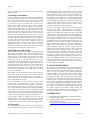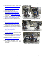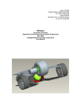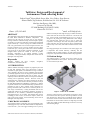
Download TailGator_IEEE_robot-FCRAR09_R1 1412KB May 01 2009 07

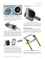
TailGator
Machine Intelligence Lab, UF
TailGator: Design and Development of
Autonomous Trash collecting Robot
Subrat Nayak 1,Bryan Hood, Owen Allen, Cory Foskey, Ryan Stevens,
Edward Kallal, Jeff Johnson, Erik Maclean, Dr. Eric M. Schwartz
Machine Intelligence Lab (MIL),
University of Florida,
325 MAE Building B, PO BOX 116300,
Gainesville FL 32611
1
Phone: (352) 392-6605
ABSTRACT
The autonomous robot discussed here was designed and built for
the 2009 IEEE SoutheastCon Hardware Competition. The
objective for the robot was to locate, pick up, sort and store
beverage containers of different shape, size and weight as quickly
as possible.. The robot was required to operate inside a designated
region bounded by a current carrying wire hidden beneath the
field. The ground surface was covered with green Astroturf. The
beverage containers were Coca-Cola products (0.5-liter plastic
bottles with caps, 8-ounce glass bottles and 12-ounce aluminum
cans) lying flat on the ground in random orientations. A well
designed robust system was needed to solve the problem.
Necessary components in our solution included a pickup
mechanism, a sorting mechanism, multiple smart sensors and an
intelligent control algorithm.
Keywords
TailGator, Grabber, Pet fence,
SoutheastCon, Autonomous, Robot
Compass,
Navigation,
email: [email protected]
different sized objects that might be lying in random orientations
and to make sure the whole robot could fit into a 12x12x18 inch
box. Several weeks of brainstorming gave rise to a variety of
designs for the picking and sorting mechanisms. Some designs
were discussed that would not robot to stop to collect the
recyclables. Some designs used rack and pinion systems while
others used belts; some tried to bring the objects perpendicularly
into the body of the robot, while others needed a two-axis robot
arm.
Several gripper designs were considered. The chosen gripper was
a compromise that ensured efficiency, reliability, met size
constraints and was simple enough to be easily fabricated using
inexpensive components and available machine shop equipments.
2.1 Platform Design
The platform (Figure 1) consists of the base, mounts for the
gripper mechanism and drive system. The base was constructed
of 1/2-inch thick acrylic sheet.
1. INTRODUCTION
Athletic stadiums and college campuses are plagued by the issue
of trash after tailgating parties, after which there is often an
assortment of glass, plastic, and aluminum beverage containers.
This is unsightly, the clean up is time consuming, and represents
a potentially significant source of untapped recyclable materials.
By developing an autonomous robot that can locate, sort, and
separately store the different containers, the manpower needed for
cleaning can be significantly reduced. With this vision, the
autonomous trash collecting robot being described in this paper
was designed. The robot was the University of Florida’s entry at
the 2009 IEEE SoutheastCon Hardware Competition [1]. Dozens
of possible solutions were considered and many experiments were
performed in order to find a solution system comprised of a
picking mechanism (that could retrieve containers placed in a
wide range of orientations), a sorting mechanism (that was not
significantly affected by environment conditions, vibrations or
deformation in the containers), simultaneous management of
Input-Output devices on an FPGA, and multiple smart sensors
(including pet fence sensors, an electronic compass, small cone
angle sonars, limit switches, current monitoring sensors and an
intelligent control algorithm).
2. MECHANICAL DESIGN
The mechanical design of TailGator robot was significantly more
challenging than any of the other IEEE hardware competitions in
at least the last 7 years. The biggest challenges were to pick up
2009 Florida Conference on Recent Advances in Robotics, FCRAR 2009
Figure 1: CAD of the PLATFORM
The drive system consists of a ball transfer unit (Figure 2) at the
front and two motor drive systems. Since the ground was covered
with Astroturf, any wheel castor or normal ball castor would get
stuck and/or restrict smooth Omni-directional motion. Hence, a
ball transfer was chosen which consists of a single large steel ball
resting on a number of small ball bearings encased in a steel cup
with mounting flanges.
Page 1 of 12
TailGator
Machine Intelligence Lab, UF
shown) were then put on the wheels to avoid any thing on the
robot touching the wheels.
Figure 2: Ball Transfer Unit– Top and Bottom View
Each motor drive system (Figure 3) consists of a motor, wheel,
hub, ball bearing and mounting bracket. The motor used is a
permanent magnet 12V DC geared motor. These motors were
chosen because their speed and torque characteristics were best
suited for our application. The extended shaft on the rear of the
motor allowed for the installation of encoders.
Figure 5: Assembled view of drive system
The gripper arm mount is made of two stands, an aluminum plate,
two aluminum angle brackets, a pin bearing and a strong high
torque low speed arm motor. The base also has two hard stops for
the gripper arms. These are made up of 10-24 threaded rods with
lock nuts.
2.2 Gripper Mechanism
Figure 3: DC geared motor
Thick Foam wheels were chosen to achieve better traction on the
Astroturf and to help in reducing the low frequency vibrations
that occurred whenever the robot traversed over wrinkles in the
Astroturf. Hub and mounting brackets (Figure 4) were machined
out of aluminum stock. The other side of the hub shaft is press fit
into a ball bearing which is again press fit into a hole on the side
bracket. This design increases the load carrying capacity of the
system.
The gripper mechanism shown in Figure 6 was used for picking
up the containers. This mechanism is comprised of two gripper
arms, atop gripper jaw and a bottom gripper jaw. These
subassemblies are capable of moving independently to perform
the motions required to pick up objects and move them to the
sorter.
Figure 4: Exploded view of drive system
Assembling the drive motor systems is done by attaching the
motor to the main mounting bracket. The hub is then attached to
the motor shaft by using the set screws and aligning it with the
motor shaft flat. The wheel is then screwed onto the hub. The
side bracket is then attached to the main bracket, and the ball
bearing is press fit into the side bracket and the hub shaft. Figure
5 shows an assembled drive system. Thin sheet metal guards (not
2009 Florida Conference on Recent Advances in Robotics, FCRAR 2009
Figure 6: Gripper mechanism for picking up objects
The right gripper arm is attached to shaft of the motor on the
gripper arm mount with an aluminum connector and a set screw.
The left gripper arm is attached to the gripper mount using a pin
Page 2 of 12
TailGator
Machine Intelligence Lab, UF
bearing and a small shaft. The right arm is actuated while the left
arm, which is free to rotate, wil follow the right arm to ensuring
mechanical support without the cost of another motor.
The upper gripper jaw (on the bottom in Figure 6) is cut from a
5–inch diameter plastic tube. The lower gripper jaw (on the top
in figure 6) is shaped from aluminum sheet metal. The jaws are
then attached to the gripper arms using custom cut aluminum
panels with servo housings and RC servos. When the servo motor
rotates the jaw moves relative to the gripper arm. The bottom jaw
is more complex in design; it has a distinctive bend in order to
temporarily hold the container after being picked up and before
being rolled down onto the sorting mechanism. This addition
solved a previously observed problem where the container hit and
became jammed against the servo body. With this addition, the
container would roll back only when the gripper jaws were raised.
This provided more time to ensure reliable identification with the
sensor that was also housed in the crevasse that was created due
to the bend.
This pick up mechanism proved to be both relatively simple and
very efficient. The open jaws cover a large area on the ground to
facilitate successful pick up of containers the different sizes
shown in Figure 7. The sensors and navigation algorithm are
expected to align the robot’s front end parallel to the container to
be picked, but neither the distance nor the orientation of the
container with respect to the gripper could be assured. This
simple gripper design generally compensated for even large errors
in the distance and alignment to allow the robot to successfully
pick up containers within a wide range of distances and
orientations. If the container is not in the desired orientation, the
gripper contributes to turning the container into the proper
orientation when the gripper jaws start closing before picking it
up.
The extreme case of container’s long end lying approximately
perpendicular to the front end of the robot should never happens
due to the navigation sensors. If were to occur, the gripper jaws
could get stuck, which will greatly increase the current. If a large
current is detected with the current sensors, the control algorithm
commands the gripper to release the container and to repeat the
navigation and pick up process.
Figure 7: Beverage containers to be picked up
2009 Florida Conference on Recent Advances in Robotics, FCRAR 2009
Two limit switches (of the type shown in Figure 8) were used at
the two extreme positions of the arm. Open loop position control
time limits were not adequate for protecting the motors. Hence, a
closed loop positioning was achieved by installing limit switches
at both extreme ends. As soon as the arm reaches a hard stop, a
switch is triggered, which signals the processor to cut power to
the motor.
Figure 8: Micro switch
2.3 Sorting Mechanism
After the pickup and identification processes are done, the gripper
rolls the container backwards along the sorter (Figure 9). The
sorting mechanism consists of the aluminum stands, plastic frame
held together by four angle brackets, collection bags and doors.
The three doors completely cover the openings, are hinged on one
side using simple loose nut-bolts, and opened/closed with a micro
servo on the opposite end. The type of container determines
which of the doors are opened and closed. The first door opens
for glass bottles, the second door opens for plastic bottle (with the
first door closed); therefore plastic bottles roll over the closed
first door. The third door is always open so that when aluminum
can is identified, the first two doors are closed and the can rolls
into the open third door. The weights of each of the containers
determined the ordering of the doors.. The entire sorter frame is
hinged onto the aluminum stands for rotational motion about a
horizontal axis. In order for the entire robot to have a maximum
starting size of 12”x12”x18”, the sorter mechanism is folded
vertically (the yellow bars in Figure 9 are rotate up approximately
90. The sorter falls open (to the configuration in Figure 9) when
the robot first moves. The position of the frame ensures a gradual
slope so that the containers will roll after falling from the grippe
jaws. The slope can be changed by two bolts that act as hard
stops. This proved to be a very simple and flexible design.
Collection bags are strapped onto the sorter frame using Velcro
straps and can be removed when filled.
Figure 9: Sorter (Note the transparent doors)
Page 3 of 12
TailGator
Machine Intelligence Lab, UF
To tackle worst case scenarios like the containers is still lying on
the sorter and didn’t roll into the right bag, the doors are opened
and closed in front of the collection bag to push them into the
correct bag. After the process is over the first two doors are
closed. (The third door is always open.)
Because of the complexity of this project, AutoDesk Inventor was
used to enable our mechanical development team to visualize and
present the mechanical design and potential problems to the rest
of the team for open discussions. All of the CAD figures in this
paper were created with this software. Figure 10 shows the final
CAD design for the robot.
Figure 12: Adjustable switching voltage regulator
3.2 SONAR
Three Devantech SRF05 sonars [4] ((Figure 13) are installed on
the front of the robot as distance sensors to locate the position of
the container to be picked up As per the rules of the 2009 IEEE
SoutheastCon Hardware Competition, the beverage containers
would never be closer than 12 inches from each other; hence,
sonars were adequate to locate the containers.
Figure 10: Fully Assembled Mechanical Hardware
3. ELECTRONIC HARDWARE
The electrical system consists of two batteries, two DC motors for
driving the wheels, one DC motor for the gripper arm, two servos
for the gripper jaws, two micro servos for the sorter doors,
voltage regulators, two pet fence sensors, three sonars, a compass,
a reflectance sensor array (identification sensor), five current
sensors, three bidirectional motor drivers for the three DC motors,
an LCD, an ATmega128 microcontroller board, and a Altera
Cyclone II FPGA board.
3.1 Power Supply
Two separate 14.8V LiPo 4450mAh battery packs are used. One
is for all the actuators and the other is for the electronics. Lithium
polymer batteries are preferable over other batteries because of
their higher energy density and lower cell count. A steady 5V
source is provided to all the electronics using a 5V, 1A switching
voltage regulator (Figure 11). A steady 7V is provided to power
the four servos using a 1A step down adjustable switching
regulator (Figure 12). [2] [3]
Figure 11: 5V, 1A switching voltage regulator
2009 Florida Conference on Recent Advances in Robotics, FCRAR 2009
Figure 13: Devantech SRF05 SONAR
For this competition, knowing the distance of an obstacle
(container) in front of the robot was not sufficient information;
the robot needed to locate these containers. Once a container was
located, the robot needed to move to an orientation that aligned
the front edge of the robot approximately parallel to the longer
edge of the container. To accomplish these tasks, three or more
distance sensors with small cone detection angle were needed.
Infrared (IR) based distance sensors were found to be less
accurate than the sonars, and were also affected by the lighting
conditions. The Devantech SRF08, Devantech SRF05 and
MaxBotix EZ2 were all tested; the SRF05 was found to have the
most narrow cone angle, the most accurate distance
measurements, and were the easiest to interface to the
microcontroller unit (MCU). We found that three of these sonars
were adequate; three sonars provided enough information without
having significant overlap of their detection cones.
The SRF05 has a transmitter and receiver tuned for 40kHz . The
transmitter sends a 40kHz ultrasonic wave and the receiver
Page 4 of 12
TailGator
Machine Intelligence Lab, UF
catches the reflected wave that bounces of an object. The distance
is measured by converting the time it takes for the pulse to return.
To communicate with the SRF05, the trigger pin (see Figure 13)
needs to be pulled high for at least 10µs (Figure 14); this sends
out the 40kHz ultrasonic wave. The echo pin remains high and
changes to low when the reflected wave is received; if nothing is
received by 30ms, then there is no object within range of the
sonar.
Biot-Savart’s Law [5] describes the magnetic effect of current
(Figure 15). The magnetic field at a point at distance r, due to a
differential element of wire of length dL, and carrying current I, is
given by
dB 
0 r I d L  r
4
r3
,
Equation 3.2.1
where µ0 is the permeability of free space/vacuum and µr is the
relative permeability of the medium.
The symbols in boldface denote vector quantities.
Figure 15: Biot-Savart’s Law
Figure 14: Interfacing the SRF05
Since we were using three SRF05s, it was necessary to ensure
that they were triggered at least 50ms apart so that the ultrasonic
wave produced by one sonar would not be detected by the next
sonar.
Therefore, the instantaneous magnetic field B (Figure 16) for a
long straight wire, carrying current I, at distance D is given by
B
0 r 2I
4 D
.
Equation 3.2.2
To ensure fast interfacing and to save MCU processing for highlevel processing, the interfacing of the various sensors was done
using an Altera Cyclone II FPGA. The FPGA logic was designed
using Altera’s Quartus using VHDL. The VHDL code utilized
one counter to hold the time taken for the signal to bounce back
and three latches, which were triggered by each of the echo lines.
When the echo returns, the current counter value was latched.
The higher the time, the farther the object was from the sonar.
3.2 Pet Fence Sensor
The “pet fence” is an invisible fence or boundary placed around
the perimeter of a home’s yard and is designed to contain the pets
within the boundaries of the property. The pet fence normally
carries a high frequency AC signal while the pet wears a light
weight receiver collar which emits a warning sound when the pet
nears the fence. If the warning is ignored and the pet approaches
even closer to the fence, the collar gives a mild electric shock to
the pet that increases in intensity as the pet moves closer to the
fence. The pet soon learns to avoid the invisible fence location,
making it an effective barrier. A pet fence was laid around the
perimeter of the robot’s designated area of operation. The robot
was supposed to remain inside this area during the entire
competition run. Since the pet fence was custom designed to
work at 10kHz and carry 25mA peak current, a ready made pet
fence collar could not be modified with additional circuitry to
give a signal to the MCU instead of the electric shock. The 10kHz
and 25mA signal was too week to directly detect since the signal
induced on an antenna is directly proportional to the frequency
and current.
2009 Florida Conference on Recent Advances in Robotics, FCRAR 2009
X: direction of magnetic field is into paper
: direction of magnetic field is out of paper
Figure 16: Magnetic field due to a long current carrying
conductor
The pet fence was arranged to form a 10ft  10ft square operating
area. Figure 17 shows the contour plot of the magnetic field
values at various points relative to a corner of the square
operating region for a constant current flowing through the pet
fence. The distance between the contour lines is not uniform and
gets smaller for points nearer to the pet fence showing that the
magnetic field is not uniformly distributed. Hence the field would
be significantly stronger and detectable at points closer to the pet
fence.
Page 5 of 12
TailGator
Machine Intelligence Lab, UF
e
Figure 17” Contour plot of the magnetic field near a corner of
the arena.
0 r 2
nAI 0 w cos(wt )
4 D
Equation 3.2.5
We see that the emf induced in a coil is directly proportional to
1) frequency of the current, 2) amplitude of the current,
3) number of turns in the coil, 4) area of cross section of the coil,
and 5) magnetic permeability of the core inside the coil. The emf
is inversely proportional to the distance from the current carrying
wire. Therefore, we decided to use a loop stick as the pet fence
sensor. The setup works like an air core transformer. The pet
fence acts as the primary winding and the sensor loop stick acts as
the secondary winding which develops an induced emf when ever
it is in the flux path. Since the frequency and current was fixed
and low, the only way to significantly increase the signal strength
of the induced emf was to make a loop stick with many of turns, a
large area of cross section and to use a high permeability core
material like ferrite rods. The loop stick also needed to be small
and light enough to be fit on the robot.
After much
experimentation, a working loop stick was made from a plastic
bobbin and thousands of turns of magnetic wire of small gauge. A
compromise was achieved to ensure that the wire was thin enough
to allow for a high number of turns, but strong enough so that it
did not break during the winding process. The magnetic wire was
wound over a bobbin using a small lathe machine and the core
was filled with ferrite rings (as shown in Figures 19 and 20).
Figure 19: Ferrite ring used for core
Figure 18: 3-D plot of the magnetic field values at various
points through out the operating region for a constant current
flowing through the pet fence
From Eq 3.2.2, the flux linked with a coil placed at a distance D
is given by
  BS  BnA 
0 r 2I
nA ,
4 D
Equation 3.2.3
where n is number of coils and A is area of cross section. Hence,
the emf (e) induced in the coil is given by
e
d 0  r 2
dI ,
nA

dt
dt
4 D
Equation 3.2.4
where only I is time varying quantity. For a sinusoidal current
waveform, I  I 0 sin(wt ) , and therefore,
2009 Florida Conference on Recent Advances in Robotics, FCRAR 2009
Figure 20: Loop Stick
The loop stick is sensitive only to magnetic fields along its axis
and hence needed to be mounted vertically as shown in Figure 20.
Two of these were needed on the front edges of the robot in order
to determine the direction of approach. The left loop stick would
conceive a higher emf than the right loop stick if the pet fence is
on the left side and vice versa.
Page 6 of 12
TailGator
Machine Intelligence Lab, UF
In reality, the current waveform in the transmitter was not
sinusoidal and contained all the odd harmonics of 10kHz. Hence,
the induced emf on the loop stick also had the odd harmonics of
10kHz in addition to from the fundamental 10kHz signal. This
was verified by viewing the Fourier transform of the induced
signal on a Digital Storage Oscilloscope. There were many other
undesired frequencies also present as noise in the induced signal.
The 20kHz motor PWM, with current much higher than the pet
fence sensor, was the major source of significantly strong noise.
The 40kHz sonars were another source of noise. Since the loop
stick is sensitive only to magnetic fields along its axis, any
vibrations or movement of the loop stick also changed the
induced voltage. This was another major source of low frequency
noise, i.e., below 10 kHz. There was no power frequency noise
because the robot was being powered with batteries. Radio
signals also caused high frequency noise.
Hence, a band pass filter was needed to isolate and sense only the
10kHz signal. A very common approach used to pick up certain
frequencies is to use parallel tuned LC circuits which resonate at
fr 
w
1

2 2 LC
.
Equation 3.2.6
But this needed accurate values of matched L and C values.
Either the desired value of the L and C could not be found or the
sizes of the components were too large. It also required constant
tuning the circuit. One solution was to use a fixed capacitor and
tune the inductor (the loop stick) by pushing a ferrite rod into the
core or manually increasing or decreasing the number of turns on
the loop stick. This process was very cumbersome and hence was
abandoned. The simpler solution was to take the induced signal
and pass it through a band-pass filter. A band-pass filter is a
device that passes frequencies within a certain range and rejects
(attenuates) frequencies outside that range.
An ideal band pass filter would have a completely flat passband
(e.g., with no gain/attenuation throughout) and would completely
attenuate all frequencies outside the passband. Additionally, the
transition out of the passband would be instantaneous in
frequency. In practice, no real band-pass filter is ideal. The filter
does not attenuate all frequencies outside the desired frequency
range completely; in particular, there is a region just outside the
intended passband where frequencies are attenuated, but not
rejected. This is known as the filter roll-off, and it is usually
expressed in dB of attenuation per decade of frequency.
Generally, the design of a filter seeks to make the roll-off as
narrow as possible, thus allowing the filter to perform as close as
possible to its intended design.
Two possible techniques for designing a steeper filter roll off are
to increase the order of the filter and to increase the quality factor
(Q) of the filter. Quality factor is defined as the center frequency
of a filter divided by the bandwidth. The bandwidth is the
frequency of the upper 3 dB roll-off point minus the frequency of
the lower 3 dB roll-off point. The higher the Q, the better is the
selectivity (see Figure 21); but with higher Q values, the filter
becomes prone to instability. [6]
2009 Florida Conference on Recent Advances in Robotics, FCRAR 2009
Figure 21: Frequency response for different vales of Quality
Factor (Q)
Band pass filters can be formed using multiple feedback op-amp
circuits or using switched capacitor filters. The design of higher
order band pass filters using op-amps were complex, required
many extra components, and required non-standard resistor
values. Use of dedicated switched capacitor filters seemed to be
the simplest solution as they needed very few extra components,
thus making the circuitry smaller and simpler. After rigorous
searching and reading trough data sheets of various switched
capacitor filter ICs, the MAXIM MAX7490 (Figure 24) was
chosen. This chip consists of two identical low-power, lowvoltage, wide dynamic range, rail-to-rail 2nd-order switchedcapacitor building blocks. Each of the two filter sections, together
with two to four external resistors, can generate all standard 2ndorder functions: bandpass, lowpass, highpass, and notch (band
reject) filters. Fourth-order filters can be obtained by cascading
the two 2nd-order filter sections (as shown in Figure 24). The
frequency response of a 4th-order filter like the one shown in
Figure 24 is shown in Figure 25. Similarly, higher order filters
can easily be created by cascading multiple MAX7490.
A switched capacitor circuit needs a clock signal for sampling.
Since the clock-to-center frequency ratio is 100:1 in the
MAX7490, a 1MHz oscillator was chosen to ensure a center
frequency at 10kHz. Sampling is done at twice the clock
frequency, further separating the centre frequency and Nyquist
frequency. [7] [8] [9] [10]
Page 7 of 12
TailGator
Machine Intelligence Lab, UF
Figure 24: Peak detector circuit
3.2 Electronic Compass
Figure 22: A 4th-order 10kHz band pass filter
To keep track of the robot’s relative orientation, the robot used a
the tilt compensated TCM2 electronic compass [12] (Figure 25)
made by PNI Sensor Corporation. This sensor provides very
accurate and noise free digital data in serial RS232 format and
can be calibrated to compensate for soft and hard iron magnetic
interferences. The orientation data, along with the pet fence
sensor data, helps in navigating in the designated area, allowing
the robot to efficiently explore the entire region. When the robot
senses the pet fence (i.e., the current carrying wire), the compass
provides the information necessary to turn the robot 90º towards
the designated area. Without the compass data, the robot may
end up following the pet fence and never explore the inner
regions of the designated area.
Figure 23: Frequency response of 4th-order 10kHz band pass
filter using MAX7490
If the two loop stick sensors are placed on either side of the pet
fence, the AC voltage induced on them will be 180º out of phase.
This fact can be used to compare the phase of the AC signals on
the two sensors and can be used to determine if the robot goes
outside of the pet fence. The induced signal, even after filtering
remains an AC signal whose amplitude represents the distance of
the sensor from the pet fence. Hence, a peak detector circuit was
needed to provide an analog DC voltage equal to the amplitude of
the input AC signal. This was accomplished by using the op-amp
circuit shown in figure 24. The DC analog voltage labeled
PeakOut was input to the MCU’s analog-to-digital converter. [11]
2009 Florida Conference on Recent Advances in Robotics, FCRAR 2009
Figure 25: TCM2 Electronic Compass
3.3 Reflectance sensor Array
One of the challenges was to differentiate between aluminum
cans, plastic bottles, and glass bottles. Overcoming this challenge
meant finding a property that distinguishes all three containers.
We chose to focus on the physical properties that can be easily
detected.
Several alternatives were considered including weight, light
absorption, and length. Since all the containers vary in length, it is
possible to sort the containers with different-sized openings. In
this design, the containers would pass over three openings of
Page 8 of 12
TailGator
Machine Intelligence Lab, UF
different size while rolling down a ramp. Only the smallest
object (can) would fall in the first opening, only the glass bottle
would fit in the second opening, and the plastic bottle would be
the only container remaining for the last opening. However, all
the containers are tapered. This means it is possible for the
tapered end of a glass or plastic bottle to jam into the smallest
opening. Hence, this design was abandoned.
Differentiating the containers based on weight requires extremely
precise sensors to accurately measure the small difference among
their weights (especially between the can and the plastic bottle).
This approach was not cost effective.
Another approach we tried was to use an infrared LED and a
phototransistor to measure the amounts of light that passed each
object. This approach was not mechanically feasible since we
found that both the LED and the photo transistor needed to touch
opposite sides of the object for successful identification. However,
this approach was incorporated in our final solution which utilizes
reflectance sensors to measure the length of the opaque (mostly
red-colored) labels (see Figure 7) on each of the Coca-Cola
(Coke) containers.
After a container is picked up, it falls into a crevasse inside the
gripper jaws where the container lies aligned with an array of
twenty reflectance sensors. The reflectance sensors measure the
length of the red coke label by determining the number of sensors
that return values below a threshold. A low value indicates an
opaque object is in front of that sensor. The number of sensors
that detect an opaque object determine the identity of the
container..
The QTR-1RC reflectance sensors [13] (Figure 26), purchased
from www.pololu.com, were used. Each sensor consists of an
infrared LED, a phototransistor, a 10nF capacitor and two
resistors (150 and 220). The schematic is shown in Figure 27.
Figure 27: QTR-1RC reflectance sensor schematic
The coke label reflects the IR light, thus reducing the resistance
of the phototransistor. The approach uses a bidirectional digital
I/O line that first charges the capacitor by making the output pin
(OUT) high for 10µs and then measuring the time for the
capacitor to discharge through the phototransistor. Shorter
discharge time implies higher reflectance or lesser resistance
between the OUT pin and ground. The discharge time is
compared to a predefined threshold value which is chosen so that
only the reflectance of the opaque label is considered reflectance.
This approach ensures higher sensitivity and lesser noise
compared to voltage-divider type resistance measuring circuits
which give analog voltage outputs.
The simultaneous reading of all 20 sensors is ensured by using
VHDL-defined components created on an Altera Cyclone II
FPGA. This facilitates quick and efficient sensing while allowing
the MCU to be used solely for high-level decision making rather
than interfacing with slow sensors. The length of the (mostly red)
opaque coke labels are measured by the number of the
consecutive sensors that sensed reflectance. The FPGA outputs
the result to the MCU through a 2-bit digital value (as shown in
Table 3.3.1). Figure 28 shows the PCB design of the reflectance
sensor array.
Table 3.3.1: Reflection sensor FPGA-uP interface
Output
Figure 26: QTR-1RC reflectance sensor (on a quarter).
00
01
10
11
Interpretation
No object
Can
Glass bottle
Plastic bottle
Figure 28: Reflection Sensor PCB Design
2009 Florida Conference on Recent Advances in Robotics, FCRAR 2009
Page 9 of 12
TailGator
Machine Intelligence Lab, UF
3.4 DC Motor Driver
The DC motors were driven in both directions using Freescale
MC33887 motor driver H-bridge ICs (Figure 29). These drivers
are capable of running DC motors at 5-28V and drawing up to
2.5A. The speed of the motor is determined by PWM signals
provided to the motor driver. The duty cycle (on-time) of the
PWM signal is proportional to the speed. The direction is chosen
by two direction pins on the motor driver (as shown in Table
3.4.1).
A parallel interface to the MCU was chosen for simplicity. The
bus consisted of eight data lines, four address lines, a read/write
signal and an enable. Internal to the FPGA, there were two buses;
one was used entirely for motor control and the other for the
sensors. Each sensor element went through a tristate buffer,
which was combined with the motor control bus at a bidirectional
buffer to the microcontroller. Each sensor element consisted of a
process block which interpreted data from various sensors and
then placed the data into a one byte register. This register could
be accessed by the MCU at any time. The motor control elements
consisted of a register and a PWM generator. The registers stored
data so that each PWM kept a desired value (proportional to the
duty cycle) until the registers were over written by a new desired
value.
3.6 ATmega128 Microcontroller
Figure 29: Dual MC33887 Motor Driver Board
Table 3.4.1: Truth Table for Direction lines
Input
00
01
10
11
The main decision making and high level algorithm were run on
an 8-bit Atmel Atmeg128 microcontroller [15] running at
16MHz. The BDMICRO Mavric IIB board [16] (Figure 31) was
selected for this purpose ATmega128 has 128K program flash,
4K static RAM, 4K EEPROM, two 8-bit timers, two 16-bit
timers, 8-channel 10-bit ADC, analog comparator, dual USARTs,
SPI, and I2C interfaces. The board also provides on-board level
shifters to offer true RS232 and RS485 voltages and has both
JTAG and ISP programming headers.
Function
Stop
ACW
CW
Never -
3.5 UF4712 Cyclone II FPGA board
An FPGA was chosen to offload data acquisition and motor
control from the microcontroller and thus allowing the MCU to
focus solely on the decision making and high level algorithms.
The UF-4712 FPGA board [14] (Figure 30) was selected. (This
board, designed by UF students, is used in UF’s Digital Design
course, EEL4712.) The UF-4712 board consists of a Altera
Cyclone II EP2C8T144C8 FPGA, two dual-digit 7-segment
displays, a ten LED bank, two 8-pin dip switch banks, and four
momentary push buttons. It also has USB connector, VGA
connector, PS/2 connector, and a JTAG programming header for
the Altera Byte Blaster.
Figure 31: Maveric IIB ATmega128 board
4. FUNCTIONING OF THE ROBOT
4.1 Initial start up
In the initial start up position of the robot, the gripper arms are
raised, and the sorter is raised to a near vertical position, giving
the robot initial starting dimensions of approximately
12”x12”x18”. In order to operate, the sorter must be lowered to
its functional position. This is accomplished by the robot quickly
accelerating forward for a short distance, and then lowering and
raising the gripper arms. If the initial forward motion of the robot
does not cause the sorter to drop, the raising of the gripper arms
will push the sorter over into its functional position.
4.2 Drive
Figure 30: UF-4712 Cyclone II FPGA board
2009 Florida Conference on Recent Advances in Robotics, FCRAR 2009
The robot is driven by applying power to the drive motors.
Providing equal power to both motors results in the robot moving
relatively straight. Turning is accomplished by varying the power
given to each drive motor. Increasing the power to the right
motor (or decreasing power to the left motor) results in a left turn.
The front ball caster can freely roll in any direction. It functions
only as third support and a means of stabilizing the robot. Using
Page 10 of 12
TailGator
this drive system, the robot is able to drive forward, reverse, and
turn left and right.
4.3 Picking up Containers
In order to pick up an object, the robot keeps moving forward
until the sonars detect the presence of some container within their
ranges. Then, using the values of the three sonars, the robot
moves towards the container, trying to align with it such that its
in front of the robot (i.e., the central sonar can detect it, the
distance of the container from the front is within a specified
range, and the longer edge of the container is approximately
parallel to the front edge of the robot). The gripper arms are then
lowered with the jaws wide open. When the arms have fully
lowered, the right arm triggers the limit switch that tells the
gripper arm motor to stop. Both arms come to rest on the hard
stops. The jaws are then closed, capturing the container. Due to
the shape of the jaws and the containers, the captured container is
forced into a parallel orientation within the jaws. In case the jaws
get stuck or the container does not allow the arm to close, the
current flowing into the gripper servos suddenly become very
high; this is detected by the current sensors and the control logic
commands the gripper to re-open. When the arm is raised to
vertical and it has reached the extreme limit, another micro switch
gets triggered that tells the gripper arm motor to stop.
4.4 Identification and Sorting
While the container is held inside the gripper jaws and the gripper
arm is raised, the container falls into a crevasse where it gets
aligned along the reflectance sensor array and is identified. Then,
based on the type of the container, the appropriate door of the
sorter mechanism is opened. The gripper jaws are then opened,
causing the container to roll back and fall on the sorting
mechanism and then rolling through the appropriate door into the
awaiting bag. This raising motion is repeated three times to
ensure that the object leaves the gripper. This repeated motion
also helps push the object over the sorter in the event of an
undesired exit from the gripper. As the gripper ramp is raised and
lowered with the gripper, the ramp can push objects into better
position to be collected.
Glass bottles will fall through the first door upon leaving the
gripper ramp. Plastic bottles will roll over the first closed door
(for glass) and fall into the second opening. Cans will roll over
both the doors (for glass and plastic containers) and fall into the
always opened third door (for cans).
Due to the possibility of an object not fully entering its proper
collection bag, a preventative measure is taken. The doors in
front of the active door is opened to help push the container into
the next door opening. In the case of a collected can, the glass
door is raised and lowered, followed by the raising and lowering
of the plastics door. This motion acts to move any object that did
not fully roll over the sorter down towards its collection bag; it
will also help to move any object that did not fully enter its bag to
complete its journey into it the proper bag and off of the sorter.
Once the above sequence is completed, the both of the two
container doors are closed. The robot then resumes its search for
additional objects. The maximum amount of objects the robot
can collect is five cans, three plastic bottles, and two glass bottles.
4.4 Navigation
Machine Intelligence Lab, UF
important navigation sensor is the pet fence sensor. If any pet
fence is detected and the left pet fence sensor has a greater value
than the right sensor, the pet fence is on the left side of the robot
and hence the robot takes a sharp 90º right turn. The robot uses
the compass to achieve the 90º turn. This navigation algorithm
helps the robot to increase the areas of exploration and discovery
than it could achieve with a blind search. Without a compass, the
turn angle cannot be guaranteed, which may cause the robot to
continue moving along the fence and never actually moving
towards the central regions of the operating area.
Since the sonars cannot see the containers from long distances,
the robot keeps moving forward expecting to encounter a
container or the pet fence. This could have been avoided and the
whole process accomplish more efficiently by using a camera that
could see from far away and guide the robot. Experiments were
performed with a USB camera that would capture 320x240 pixel
sized pictures of the field and look for the color red. Each object
had a significant portion of red on its label that was easily
distinguished from a green background with our image processing
algorithms. In order to reduce the effects from lighting, the
images in RGB space images were converted to HSV space.
Simply looking at the hue values in the image and applying a
double threshold to isolate the red hue, a binary image was
produced that contained only the red labels. Then, using contour
finding algorithms, the individual objects were located. The
container lying lowest on the image was the nearest to the robot
and was the first target. All the image processing was done using
the OpenCV computer vision processing library [17] on an
embedded computer board that was supposed to be housed on the
robot. The embedded computer was to communicate with the
micro controller board via serial RS232 protocol. But due to
complexity of the system, and the success of the sonar system, the
use of the camera was discarded.
5. ACKNOWLEDGMENTS
We would like to thank IEEE Atlanta Section and Georgia Tech
IEEE student branch for hosting the 2009 IEEE SoutheastCon
Hardware Competition, which motivated us to work hard for this
project. We are also grateful to the Machine intelligence
Laboratory (MIL) at UF, where all of the research, design,
testing, and most of the construction occurred. We wish to thank
the IEEE Gainesville section and Gainesville section student
branch at UF for providing us the funds to turn our ideas into a
functioning robot. We express our special gratitude to our faculty
advisors for all their support, encouragement and advice. We are
also thankful to STMicroelectronics, Maxim, Texas Instruments
and Linear Technologies for providing free samples of various
ICs. Finally, we are indebted to other members of the MIL and
the teaching assistants of EEL4924C (Senior Design) and
EEL5666C (Intelligent Machines Design Laboratory) courses
who helped us with advices, resources and encouragement.
6. REFERENCES
[1] “IEEE SoutheastCon2009 Hardware competition Rules and
Transmitter,”August 2008.
[2] Dimension Engineering DE-SWADJ Adjustable Switching
Voltage Regulator data sheet,
http://www.dimensionengineering.com/DE-SWADJ.htm
The primary navigation sensor of the robot is the sonar. The robot
locates and aligns with containers using the sonars. The next
2009 Florida Conference on Recent Advances in Robotics, FCRAR 2009
Page 11 of 12
TailGator
[3] Dimension Engineering DE-SW050 5v Switching Regulator
data sheet,
http://www.dimensionengineering.com/DE-SW050.htm
Machine Intelligence Lab, UF
7. ROBOT PICTURES
[4] “SRF05 - Ultra-Sonic Ranger Technical Specification,”
http://www.robot-electronics.co.uk/htm/srf05tech.htm
[5] David J. Griffiths, Introduction to Electrodynamics (3rd
Edition), Prentice-Hall, London, 1999.
[6] MAXIM application note 733: “A Filter Primer,”
http://www.maxim-ic.com/appnotes.cfm/an_pk/733/
October 2008.
[7] Bruce Carter, “A Single-Supply Op-Amp Circuit Collection”
(Texas Instruments), http://www.ti.com/litv/pdf/sloa058
November 2000.
[8] Ron Mancini, “Op Amps for Everyone” (Texas Instruments),
http://focus.ti.com/lit/an/slod006b/slod006b.pdf 2002.
[9] “MAXIM MAX7490 Dual Universal Switched-Capacitor
Filters,” http://www.maxim-ic.com/quick_view2.cfm/
qv_pk/2325 2007.
Figure 31: TailGator in home position (left) and with sorting
mechanism deployed (right)
[10] MAXIM application note 3494: “The Basics of AntiAliasing: Using Switched-Capacitor Filters,”
http://www.maxim-ic.com/appnotes.cfm/an_pk/3494/
April 2005.
[11] Ramakant Gayakwad, Op-Amps and Linear Integrated
circuits (4th edition), Prentice Hall, London, August 1999.
[12] “TCM2 Electronic Compass Module User’s Manual” (PNI
Sensor Corporation), http://www.pnicorp.com/files/
TCM2.5_31-March-2009.pdf April 2002.
[13] “Pololu QTR Reflectance Sensor Application Note,”
http://ww.pololu.com/docs/pdf/0J13/
QTR_application_note.pdf 2009.
[14] Eric M. Schwartz, et al., “UF-4712 Board Manual” Revision
1.7, http://www.mil.ufl.edu/4712/docs/uf-4712_board/UF4712_Board_Manual_v1.7.pdf, from UF’s EEL4712: Digital
Design, September 2008.
Figure 32: TailGator with grabber fully open (left) and
partially open (right)
[15] “Atmel ATmega128: 8-bit AVR Microcontroller with 128K
Bytes In-System Programmable Flash,” www.atmel.com/
atmel/acrobat/doc2467.pdf June 2008.
[16] “BDMICRO MAVRIC-IIB ATMega128 AVR Integrated
Controller II Technical Manual” Revision B,
http://www.bdmicro.com/mavric-iib/mavric-iib.pdf, March
2009.
[17] Gary Bradski and Adrian Kaehler, Learning OpenCV:
Computer Vision with the OpenCV Library, O’Reilly,
September 2008.
Figure 33: TailGator in container retrieval position
2009 Florida Conference on Recent Advances in Robotics, FCRAR 2009
Page 12 of 12