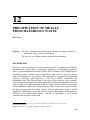
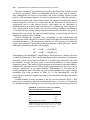
1
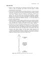
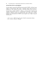
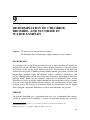
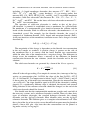
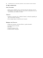
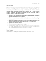
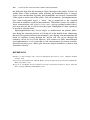
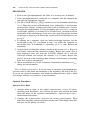
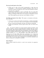
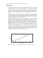
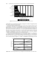
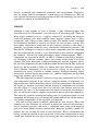
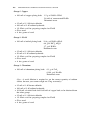
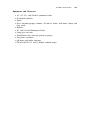
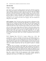
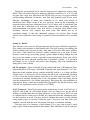
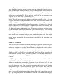
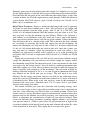
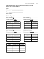
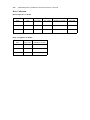
88
CONCENTRATION OF CHLORINATED PESTICIDES IN WATER SAMPLES
GC Conditions
1.0-mL injection
Inlet temperature ¼ 270 C
Column:
HP-1 (cross-linked methyl silicone gum)
30.0 m (length) by 530 mm (diameter) by 2.65 mm (film thickness)
4.02-psi column backpressure
3.0-mL/min He flow
31-cm/s average linear velocity
Oven:
Hold at 180 C for 1.0 minute
Ramp at 5.0 C/min
Hold at 265 C for 16.0 minutes
Total time ¼ 34.0 minutes
Detector:
Electron-capture detector
Temperature ¼ 275 C
Makeup gas ¼ ArCH4
Total flow ¼ 60 mL/min
Retention times (from Figure 8-1) for the given GC setting are:
Lindane
12.13 minutes
Aldrin
16.86 minutes
2,20 ,4,40 ,6,60 -TCB
18.86 minutes
Endosulfan I (IS)
19.75 minutes
Dieldrin
20.95 minutes
PROCEDURE
89
PROCEDURE
1. Obtain a water sample from your laboratory instructor. The water sample
will be a 500- or 1000-mL glass bottle and will contain a known
concentration of each analyte.
2. Set up your extraction apparatus according to Figure 8-2. Soap-wash and
water-rinse all glassware that will be contacting your sample to remove
interfering compounds (especially phthalates from plastics). Remove any
water with a minimal amount of pesticide-grade methanol or acetone.
Finally, rinse the glassware with pesticide-grade methylene chloride.
Deposite rinse solvents in an organic waste bottle, not down the sink drain.
3. Fill the drying column with anhydrous Na2SO4 (a 3- to 4-inch column of
Na2SO4 will be sufficient).
4. Pour the contents of your sample container into your separatory funnel.
Add about 25 mL of methylene chloride to your original sample container,
cap it, and shake for 30 seconds. (The purpose of this step is to remove any
analyte that may have sorbed to the surface of your sample container.)
5. Quantitatively transfer the methylene chloride from your sample container
to the separatory funnel. Add about 1 g of NaCl to your water sample in
the separatory funnel (this will inhibit the formation of an emulsion layer
that could form between the two liquid layers and interfere with your
transfer to the drying column). Seal the funnel, shake vigorously for
2 minutes, releasing the pressure as necessary, and allow the layers to
separate. Swirl the funnel as needed to enhance the separation and remove
methylene chloride from the separatory funnel walls.
Figure 8-2. Extraction setup held in place with a ring stand.
90
CONCENTRATION OF CHLORINATED PESTICIDES IN WATER SAMPLES
6. Carefully open the stopcock and allow only the bottom layer (methylene
chloride) to enter the drying column. Be careful not to let any water phase
enter the drying column since excessive amounts of water will clog
this column. The methylene chloride should pass uninhibited into the
100.0-mL volumetric flask.
7. Add about 25 mL of methylene chloride to your sample container and
repeat steps 4 through 6 two more times, collecting each extract into the
100.0-mL volumetric flask. (As you add methylene chloride to the drying
column, you may occasionally need to break up the surface of the column.
Water contained in the methylene chloride will be removed from the
organic layer and bound to the Na2SO4, forming a crust on the surface.)
8. Rinse the drying column with additional methylene chloride and fill your
100-mL volumetric flask to the mark.
9. The concentration in your water sample and methylene chloride extract is
very low and needs to be concentrated to measure the concentration
adequately. We will concentrate your extract using a warm water bath
and a gentle flow of N2 (or He). Pipet 10.00 mL of your 100.0-mL extract
into a graduated 10- or 15-mL thimble. We will check the recovery of this
step using an internal standard, Dieldrin. Using a microsyringe, add
exactly 2.00 mL of an 80.0-ppm Dieldrin solution supplied by your
laboratory instructor. Place the thimble in a warm water bath and adjust
a gentle stream of nitrogen or helium over the surface of the liquid. The
gas stream will evaporate the liquid.
10. After the liquid level has reached 1 mL, pipet 5.00 mL more of your
extract into the thimble (this will give you a total of 15.0 mL). Gently
evaporate the liquid to dryness, remove immediately, and add isooctane
and your GC internal standard. First, pipet 2.00 mL of isooctane into the
thimble. The GC internal standard is Endosulfan I. Using another microsyringe, add 2.00 mL of an 80.0-ppm solution. Using a clean Pasteur pipet,
rinse the walls of the thimble from top to bottom several times. This will
redissolve any analyte or internal standards that precipitated on the walls
of your thimble. The final concentration of each internal standard is
32.0 ppb.
11. Transfer the isooctane extract to a GC autoinjection vial or cap your
thimble until you analyze it on the GC.
12. Sign into the GC logbook and analyze your samples using the conditions
given under ‘‘GC Conditions’’ in the section ‘‘In the Laboratory.’’ When
you finish, record any instrument problems in the logbook and sign out.
Waste Disposal
All organic liquids should be disposed of in an organic hazardous waste
receptacle. These solutions will be disposed of properly by the safety officer.
ASSIGNMENT
91
ASSIGNMENT
After you analyze your samples, calculate the concentration of each analyte in
your original water sample. Calculate a standard deviation using data acquired by
the entire class. Using the Student t-test spreadsheet (see Chapter 2) and the
known value provided by your instructor, determine if bias is present in your
analysis.
92
CONCENTRATION OF CHLORINATED PESTICIDES IN WATER SAMPLES
ADVANCED STUDY ASSIGNMENT
A water sample is extracted for DDT and analyzed by GC–ECD. A 500-mL water
sample is extracted three times using a separatory funnel and the extract is
combined to a final volume of 100.0 mL. A 20.00-mL aliquot of the 100.0 mL is
concentrated to 1.00 mL. Dieldrin is added as a recovery check standard to the
1.00-mL concentrated extract at a concentration of 50.0 ppb. A GC internal
standard is added to correct for injection errors and is recovered at 95.0%.
Calculate the concentration of DDT in your original water sample using the
following data:
GC results for DDT: 45.6 mg/L in the 1.00-mL concentrated solution
GC results for Dieldrin: 48.5 mg/L
9
DETERMINATION OF CHLORIDE,
BROMIDE, AND FLUORIDE IN
WATER SAMPLES
Purpose: To learn to use ion-specific electrodes
To determine the concentration simple anions in water samples
BACKGROUND
As rainwater falls on the Earth and contacts soil, it dissolves minerals, which are
washed into streams and lakes. These waters, in turn, transport a variety of cations
and anions to the oceans. Over millions of years, this resulted in the high salt
content of ocean water. Common cations include sodium, potassium, calcium, and
magnesium; common anions are chloride, sulfate, carbonate, bicarbonate, and
nitrate, although other cations and anions may be present, depending on the local
geologic media. Some ions are nutrients; others may be potentially toxic. In this
laboratory we use a relatively simple method for measuring the activity of anions
in water. Note that electrodes measure activity, not concentration. In low–ionic
strength waters, the activity is essentially equal to concentration, but for higher
ionic strengths, important differences in these measurements are present.
THEORY
Ion-specific electrodes are a convenient and easy way to determine the concentration of certain ions in solution. A variety of electrode designs are available,
Environmental Laboratory Exercises for Instrumental Analysis and Environmental Chemistry
By Frank M. Dunnivant
ISBN 0-471-48856-9 Copyright # 2004 John Wiley & Sons, Inc.
93
94
DETERMINATION OF CHLORIDE, BROMIDE, AND FLUORIDE IN WATER SAMPLES
including (1) liquid membrane electrodes that measure Ca2þ, BF4, NO3,
ClO4, Kþ, Ca2þ, and Mg2þ (water hardness); (2) gas-sensing probes that
measure NH3, CO2, HCN, HF, H2S, SO2, and NO2; and (3) crystalline membrane
electrodes (solid-state electrodes) that measure Br, Cd2þ, Cl, Cu2þ, F, I,
Pb2þ, Ag/S2, and SCN. We use the latter, solid-state electrodes to measure Cl,
Br, and F ion concentrations.
The operation of solid-state electrodes is similar to that of the glass,
pH electrode. A potential is established across a membrane. In a pH electrode,
the membrane is a semipermeable glass interface between the solution and the
inside of the electrode, while in solid-state electrodes, the membrane is a 1- to
2-mm-thick crystal. For example, for the fluoride electrode, the crystal is
composed of lanthanum fluoride (LaF3) doped with europium fluoride (EuF2).
At the two interfaces of the membrane, ionization occurs and a charge is created
described by
LaF3 ðsÞ $ LaFþ
2 ðsÞ þ F ðaqÞ
The magnitude of this charge is dependent on the fluoride ion concentration
in the test sample or standard. A positive charge is present on the side of
the membrane that is in contact with the lower fluoride ion concentration,
while the other side of the membrane has a negative charge. The difference in
charge across the membrane allows a measure of the difference in fluoride
concentration between the two solutions (inside the electrode and in the test
solution).
The solid-state electrodes are governed by a form of the Nernst equation,
E¼Kþ
0:0592
pX
n
ð9-1Þ
where E is the voltage reading, K an empirical constant (the y intercept of the logactivity or concentration plot), 0.0592/n the slope of the line [0:0592 ¼ RT=F
ðR ¼ 8:316 J/molK, T in temperature in kelvin, and F ¼ 96487 C/mol)], and pX
is the negative log of the molar ion concentration. Note that for monovalent ions
(an n value of 1), the slope should be equal to 0.0592 if the electrode is working
properly. If a significantly different slope is obtained, the internal and external
filling solutions of the reference electrode should be changed, or the end of the
solid-state electrode should be cleaned.
You should note that the semipermeable membrane provides only one-half of
the necessary system, and a reference electrode is needed. There are three basic
types of reference electrodes: the standard hydrogen electrode, the calomel
electrode, and the Ag/AgCl electrode. Most chemists today use the Ag/AgCl
reference electrode. This addition gives us a complete electrochemical cell. Note
that a plot of the log of ion activity versus the millivolt response must be plotted to
obtain a linear data plot. Also note that the concentration can be plotted as
log(molar activity) or log(mg/L).
REFERENCES
95
REFERENCES
Skoog, D. A, F. J. Holler, and T. A. Nieman, Principles of Instrumental Analysis, Saunders College
Publishing/Harbrace College Publishers, Philadelphia, 1998.
Willard, H. H., L. L. Merritt, Jr., J. A. Dean, and F. A. Settle, Jr., Instrumental Methods of Analysis,
Wadsworth, Belmont, CA, 1988.
96
DETERMINATION OF CHLORIDE, BROMIDE, AND FLUORIDE IN WATER SAMPLES
IN THE LABORATORY
Safety Precautions
Safety glasses should be worn at all times during the laboratory exercise.
The chemicals used in this laboratory exercise are not hazardous, but as in
any laboratory, you should use caution.
Chemicals
Sodium or potassium salts of chloride, bromide, or fluoride (depending on
the ion you will be analyzing)
Ionic strength adjustor (consult the user’s manual)
Equipment and Glassware
Solid-state electrodes (each ion will have a specific electrode)
Ag/AgCl reference electrode
mV meter
Standard volumetric flasks
Standard beakers and pipets
PROCEDURE
97
PROCEDURE
The exact procedure will depend on the brand of electrode you are using. Consult
the user’s manual. In general, you will need an ionic strength adjustor that does
not contain your ion of interest, a single- or double-junction reference electrode
(specified in the solid-state electrode user’s manual), and a set of reference
standards made from the sodium or potassium salts. In general, the range of
standards should be from 0.50 to 100 mg/L.
1. First, set up your electrodes and allow them to equilibrate in the solution for
the time specified in the user’s manual.
2. Make up your reference standards and analyze them from low to high
concentration.
3. Make a plot according to equation (9-1) (mV versus the negative log of your
analyte concentration) and ensure that the slope is at or near 59.2.
4. Analyze your unknown samples.
5. Calculate the concentration in your samples.
6. Disassemble the setup. Dry off the solid-state electrode and return it to its
box. Empty the filling solution of the reference electrode, wash the outside
and inside with deionized water, and allow it to air dry.
Waste Disposal
All solutions can be disposed of down the drain with excess water.
98
DETERMINATION OF CHLORIDE, BROMIDE, AND FLUORIDE IN WATER SAMPLES
ASSIGNMENT
Use the Excel spreadsheet to analyze your data. Calculate the concentration of
analytes in your samples.
ADVANCED STUDY ASSIGNMENT
99
ADVANCED STUDY ASSIGNMENT
Research solid-state electrodes. Draw a complete electrode setup, including a
cross section of a solid-state electrode and a cross section of an Ag/AgCl
reference electrode.
DATA COLLECTION SHEET
10
ANALYSIS OF NICKEL SOLUTIONS
BY ULTRAVIOLET–VISIBLE
SPECTROMETRY
SAMANTHA SAALFIELD
Purpose: To determine the concentration of a transition metal in a clean aqueous
solution
To gain familiarity with the operation and applications of an
ultraviolet–visible spectrometer
BACKGROUND
When electromagnetic radiation is shown through a chemical solution or liquid
analyte, the analyte absorbs specific wavelengths, corresponding to the energy
transitions experienced by the analyte’s atomic or molecular valence electrons.
Ultraviolet–visible (UV–Vis) spectroscopy, which measures the absorbent behavior of liquid analytes, has in the last 35 years become an important method for
studying the composition of solutions in many chemical, biological, and clinical
contexts (Knowles and Burges, 1984).
UV–Vis spectrometers operate by passing selected wavelengths of light
through a sample. The wavelengths selected are taken from a beam of white
light that has been separated by a diffraction grating. Detectors (photomultiplier
tubes or diode arrays) report the amount of radiation (at each wavelength)
transmitted through the sample. The peaks and troughs of absorption at different
wavelengths for a particular analyte are characteristic of the chemicals present,
and the concentration of chemicals in the sample determines the amount of
Environmental Laboratory Exercises for Instrumental Analysis and Environmental Chemistry
By Frank M. Dunnivant
ISBN 0-471-48856-9 Copyright # 2004 John Wiley & Sons, Inc.
101
102
ANALYSIS BY ULTRAVIOLET–VISIBLE SPECTROMETRY
radiation reaching the detector. Thus, for a given solution, the wavelength of
maximum absorption (lmax) remains constant, while the percent transmittance
increases and the absorbance decreases as the solution is diluted (as will be seen
in this experiment).
Major limitations of UV–Vis spectroscopy result from the nonspecific nature of
the instrument. Spectrometers simply record how much radiation is absorbed,
without indicating which chemical species is (are) responsible. Thus, spectroscopy is most valuable in analyzing clean solutions of a single known species
(often at different concentrations, as studied in this experiment), or analytes such
as plating solutions, which have only one (metal) species that will absorb visible
light. Procedures for activating a particular species, or giving it color through
chemical reaction, can also make spectroscopy useful for analyzing complex
matrices.
UV–Vis spectroscopy has various applications in environmental chemistry. For
plating solutions, knowing the amount of metal present in waste determines
treatment procedures. Complex extraction and digestion procedures are also used
to determine the concentrations of species, from iron to phosphate, in soils,
sediments, and other environmental media.
THEORY
The relationship between absorbance and concentration for a solution is expressed
by Beer’s law:
A ¼ ebc ¼ log T
ð10-1Þ
where A is the absorbance by an absorbing species, e the molar absorptivity of the
solution, independent of concentration (L/molcm), b the path length of radiation
through cell containing solution (cm), and c the concentration of the absorbing
species (mol/L). Thus, when the molar absorptivity (dependent on the atomic or
molecular structure) and path length are held constant, the absorbance by an
analyte should be directly proportional to the concentration of the absorbing
species in the analyte. This leads to a linear relationship between concentration
and absorbance and allows the concentration for unknown samples to be
calculated based on plots of data for standards of known concentrations. If
more than one absorbing species is present, the absorbance should be the sum of
the absorbances of each species, assuming that there is no interaction between
species.
Beer’s law generally holds true for dilute solutions (where absorbance is less
than 3). At higher concentrations, around the limit of quantitation, the plot of
concentration versus absorbance levels out. This occurs as the absorbing species
interferes with itself so that it can no longer absorb at a rate proportional to its
concentration. A leveling out of the Beer’s law plot may also be observed at very
low concentrations, approaching the limit of linearity and the detection limit of
the instrument.
THEORY
103
The absorbance of electromagnetic radiation by chemical compounds in
solution results from the transitions experienced by the compounds’ electrons
in response to the input of photons of distinct wavelengths. Organic compounds
often contain complex systems of bonding and nonbonding electrons, most of
which absorb in the vacuum–UV range (less than 185 nm). Functional groups that
allow excitation by, and absorbance of, radiation in the longer UV or visible
wavelengths are called chromophores. For example, unsaturated functional
groups, containing nonbonding ðnÞ or pi-orbital (p) electrons, absorb between
200 and 700 nm (often in the visible range) as they are excited into the
antibonding pi orbital ðp Þ.
The absorption of visible radiation by light transition metals leads to primary
applications of spectroscopy to inorganic compounds. These metals have a
characteristic set of five partially filled d orbitals, which have slightly different
energies when the metals are complexed in solution. This enables electronic
transitions from d orbitals of lower to higher energies. In solutions of divalent
metals with nitrate, such as the solution of Ni(NO3)2 6H2O that we study in this
experiment, six water molecules generally surround the dissolved metal in an
octahedral pattern (Figure 10-1). The negative ends of these molecules, aligned
toward the unfilled d orbitals of the metal, repel the orbitals and thus increase their
energy. However, due to the distinct orientations of the various d orbitals around
the nucleus, some are more affected than others by this repulsion. The relatively
small resulting energy differences correspond to photons in the visible range. For
lightweight transition metals, these wavelengths vary according to the solvent (in
this experiment, water) and resulting ligand (Ni(H2O)62; in contrast, the spectra
for lanthanide and actinide metals have sharper peaks and are generally independent of solvent. Overall, the subtle d-orbital splitting in transition metal solutions
gives these solutions their colors and makes them valuable candidates for visible
spectrometric analysis.
Although all spectrophotometers operate on the same principles, they have a
number of variations that affect their operation and analytical flexibility. Some
instruments have adjustable bandwidths, which allow you to change the amount of
Figure 10-1. Model of octahedral nickel ion–water complex.
104
ANALYSIS BY ULTRAVIOLET–VISIBLE SPECTROMETRY
the diffracted light that the instrument allows through to the sample. Narrow slit
widths allow a finer resolution, while widening the bandwidth gives a stronger
signal. One consideration regarding both bandwidths and analyte concentrations
is the signal-to-noise ratio of the results. Like all instruments, spectrophotometers
have some background signal, a ‘‘noise’’ that is manifested as the standard
deviation of numerous replicate measurements. With either narrow slit widths or
lower concentrations, the signal-to-noise ratio (average reading/standard deviation) may increase due to a decrease in the signal, although this is more significant
in regard to concentrations.
Spectrophotometers may also be single- or double-beam, the primary difference being the continual presence of a blank cell in the double beam, eliminating
the need for repeated reference measurements, since during each measurement the
beam of radiation passing through the analyte cell also passes through the
reference cell on its way to the detector. Also, whereas in older, nonautomated
spectrophotometers it was preferable to take measurements of percent transmittance because they gave a linear plot, on newer digital machines it is fine to read
absorbance directly.
REFERENCES
Knowles, A. and C. Burges (eds.), Practical Absorption Spectrometry, Vol. 3, Chapman & Hall,
London, 1984.
Sawyer, D. T., W. R. Heineman, and J. M. Beebe, Chemistry Experiments for Instrumental Methods,
Wiley, New York, 1984.
Skoog, D. A., J. F. Holler, and T. A. Nieman, Principles of Instrumental Analysis, 5th ed., Harcourt
Brace College Publishing, Philadelphia, 1998.
IN THE LABORATORY
105
IN THE LABORATORY
Chemicals
ACS-grade crystalline Ni(NO3)2 6H2O
Equipment and Glassware
Spectrophotometer (automated is preferable, but a Spectronics 20 will
work), with visible radiation lamps
Analytical balance
Five 25-ml volumetric flasks per student or pair of students
1-mL, 2-mL, 4-mL, and 10-mL pipets
Matched cuvettes for visible light
Preparation of Standards
0.250 M Ni(NO3)2 6H2O: Dissolve about 1.82 g of crystalline Ni(NO3)2 6H2O in deionized water in a 25-mL volumetric flask. Record the actual
weight of Ni(NO3)2 6H2O added, to calculate the actual concentration.
Dilutions: 0.0100 M, 0.0200 M, 0.0400 M, and 0.100 M Ni(NO3)2 6H2O:
Pipet 1.00 mL, 2.00 mL, 4.00 mL, and 10.00 mL of 0.250 M Ni(NO3)2 6H2O, respectively, into 25-mL volumetric flasks. These and the remaining
0.250 M solution can be stored in covered beakers if necessary or to make
them easier to transfer.
106
ANALYSIS BY ULTRAVIOLET–VISIBLE SPECTROMETRY
PROCEDURE
1. Turn on the spectrophotometer and allow it to warm up for 20 minutes.
2. If the spectrophotometer is connected to a computer, turn the computer on
and open the appropriate program.
3. Use the 0.100 M Ni(NO3)2 6H2O solution to test for maximum absorbance
(lmax). Rinse the cuvette with deionized water, followed by a small portion
of the analyte solution, and then pour about 3 mL of solution into a cuvette.
Zero the spectrophotometer. If your instrument will scan across a range of
wavelengths, perform a scan from 350 to 700 nm. If not, you need to test the
absorbance of the solution every 5 nm across this range. Record the location
of the largest, sharpest peak. Retain the cuvette with 0.100 M nickel for use
in step 5.
4. If working on a computer, open the fixed-wavelength function. Set the
wavelength to the lmax you found in step 3 on either the computer or
the manual dial. If bandwidth is adjustable, set it at 2 nm. Rezero the
instrument.
5. Analyze the 0.100 M nickel solution already in the cuvette at lmax. Repeat 5
to 10 times, and record the absorbance readings. Empty the cuvette, rinse it
with deionized water and with the 0.0100 M solution, fill it with the
0.0100 M solution, and analyze the contents 5 to 10 times. Repeat this
process for each of the remaining three solution concentrations, proceeding
from least to most concentrated.
6. Obtain an unknown in a 25-mL volumetric. Determine it absorbance at lmax,
taking five measurements.
Note on blank measurements: If you are using an automatic spectrophotometer,
you only need to take blank measurements at the beginning and end of the day.
If you are on a manual instrument, take blank measurements often, such as when
you change solutions or parameters of measurements.
Optional Procedures
Signal-to-Noise Ratio
1. Analyze three or more of the nickel concentrations at least 20 times,
recording each absorbance, and calculate the mean and standard deviation
about the mean of the repetitive measurements. (signal-to-noise ratio ¼
mean/standard deviation).
2. Compare the signal-to-noise ratios for the various concentrations. What
effect does changing concentration have on the ratio? What implication does
that have for the quality of results?
PROCEDURE
107
Wavelength and Signal-to-Noise Ratio
1. Analyze one or more of the nickel concentrations at more than one
wavelength (lmax and at least one at nonpeak absorbance) with at least 20
repetitions for each wavelength. Be sure to rezero the instrument each time
you change the wavelength.
2. Compare the absorbance at various wavelengths. Does the trend make
sense? Compare the signal-to-noise ratios for the same concentration at
different wavelengths. What effect does changing wavelength have on the
ratio? What implication does that have for the quality of results?
Slit Width and Signal-to-Noise Ratio. This requires an instrument with adjustable bandwidths.
1. Analyze two or more of the nickel concentrations at multiple bandwidths
(e.g., 0.5 nm, 2 nm, 10 nm), with at least 20 repetitions for each bandwidth.
Be sure to rezero the instrument each time you change the bandwidth.
2. Compare the absorbances and the signal-to-noise ratios for various bandwidths.
Note: To conserve solutions in carrying out these optional procedures, work
with one solution at a time by incorporating these procedures into step 5 of the
main procedure. [The frequent changing of settings (precedents) that this requires
may make it difficult on a Spectronics 20 (nonautomated) system.] For example, if
you plan to complete all the procedures, when you get to step 5, scan the 0.100 M
solution 20 times (at l ¼ lmax and bandwidth ¼ 2 nm). Then change the wavelength and scan 20 times again. Return the wavelength to lmax, change the
bandwidth, and scan at 0.5 nm and then at 10 nm. Restore the original settings and
proceed to the other solutions, carrying out as many of the optional procedures as
desired. The most important thing to remember is to rezero the instrument each
time you change the wavelength or bandwidth.
Waste Disposal
Nickel solutions should be placed in a metal waste container for appropriate
disposal.
108
ANALYSIS BY ULTRAVIOLET–VISIBLE SPECTROMETRY
ASSIGNMENT
1. Create a Beer’s law plot similar to the one shown in Figure 10-2, relating
nickel concentration (x axis) to mean absorbance ( y axis) for the standard
solutions. Be sure to use the actual concentrations of the solutions you made
if they varied from the stated value. Turn in a copy of this plot along with a
short table of the corresponding data (mean absorbances and concentrations).
2. Complete a linear least squares analysis on the Beer’s law plot, using the
statistical template spreadsheet provided on the included CD-ROM or from
your instructor. Turn in a copy of the spreadsheet with a short discussion of
what the analysis indicates about your data.
3. Evaluate your unknowns. After you have entered the data for the standards
into the ‘‘LLS’’ spreadsheet, enter the absorbances (‘‘signals’’) of the
unknowns into the bottom of the sheet. Transfer the concentrations calculated by Excel for these absorbances into the ‘‘t-test’’ sheet (‘‘observation’’
column). Enter the number of replicates (N), and set the desired degrees of
freedom (usually, N 1) and the confidence interval. Fill in the true
unknown concentrations provided by your instructor, and consult the
statistical test to see whether bias is present in your measurements. Include
a copy of the spreadsheets in your lab manual with a short discussion of
what this test indicates and of possible sources of discrepancy between your
calculated concentration values and the true values.
1.4
y = 4.53236x + 0.05786
R2 = 0.994
Absorbance
1.2
1
0.8
0.6
0.4
0.2
0
0.0000
0.0500
0.1000
0.1500
0.2000
0.2500
0.3000
Concentration (M)
Figure 10-2. Example of typical student data: Beer’s law plot for Ni(NO3)2 6H2O.
ADVANCED STUDY ASSIGNMENT
109
ADVANCED STUDY ASSIGNMENT
Hand-draw a spectrophotometer. Label the components and explain briefly
operation of the instrument.
DATA COLLECTION SHEET
PART 4
EXPERIMENTS FOR
HAZARDOUS WASTE
11
DETERMINATION OF THE
COMPOSITION OF UNLEADED
GASOLINE USING GAS
CHROMATOGRAPHY
Purpose: To learn to use a capillary column gas chromatography system
To learn to use column retention times to identify compounds
To learn to calibrate a gas chromatograph and quantify the mass of
each peak
BACKGROUND
Petroleum hydrocarbons may well be the most ubiquitous organic pollutant in the
global environment. Every country uses some form of hydrocarbons as a fuel
source, and accidental releases result in the spread and accumulation of these
compounds in water, soil, sediments, and biota. The release of these compounds
from underground storage tanks is the most common release to soil systems, and
this is discussed in Chapter 16. The drilling, shipping, refining, and use of
petroleum products all account for serious releases to the environment.
Crude oil consists of straight-chained and branched aliphatic and aromatic
hydrocarbons. Upon release into the environment, some compounds undergo
oxidation. Chemical and photochemical oxidation occur in the atmosphere; in
water and soil systems, microorganisms are responsible for the oxidation. The
analysis of crude oil, and organic compounds in general, has improved enormously with the advent of capillary column gas chromatography. In fact, capillary
Environmental Laboratory Exercises for Instrumental Analysis and Environmental Chemistry
By Frank M. Dunnivant
ISBN 0-471-48856-9 Copyright # 2004 John Wiley & Sons, Inc.
113
114
COMPOSITION OF UNLEADED GASOLINE USING GAS CHROMATOGRAPHY
Norway
Venezuela
United Kingdom
Iran
Indonesia
Canada
Saudi Arabia
China
Russia
United States
0
10
20
30
40
50
60
70
Quadrillion BTU per year
Oil
Natural Gas
Coal
Figure 11-1. Energy production of selected countries. (U.S. EPA, 2002.)
column GC can even identify the country of origin of a crude oil sample based on
the chemical/compound composition.
One of the largest problems with respect to the release of hydrocarbons in the
environment is that they are hydrophobic (they do not like to be in water).
Hydrocarbons are organic compounds and do not undergo hydrogen bonding, and
thus do not readily interact with water. As a result, hydrocarbons bioaccumulate in
the fatty tissue of plants and animals or associate with organic matter in soils and
sediments. Compounds can be toxic at low levels, one of the most common
examples being benzene, present in all gasoline products.
Our use of petroleum hydrocarbons is ever-increasing. Figure 11-1 summarizes
the production rates for the highest-energy-consuming countries. You will note
that the United States produces (and consumes) the most energy per year. But how
do we use this energy? Figure 11-2 shows a breakdown of the energy use into
Million barrels per day
20
72%
15
67%
10
Transportation
53%
Industrial
5
Residential and commercial
Electric Utility
0
1970
1980
1990
2000
2010
2020
Figure 11-2. Current and predicted energy consumption in the United States. (U.S. EPA, 2002.)
THEORY
115
electric, residential and commercial, industrial, and transportation. Transportation, the largest form of consumption, is increasing at an alarming rate. This not
only explains the intensive research programs in fuel cell technology but also the
geopolitical conflicts in the Middle East.
THEORY
Although it takes months to years to become a good chromatographer, this
laboratory exercise will introduce you to the basics of chromatography. There are
many highly technical parts to a capillary column GC, including the ultrapure
carrier and makeup gases, flow controller values, injector, column, oven, a variety
of detectors, and a variety of data control systems. You should consult a textbook
on instrumental methods of analysis for details on each of these systems. The
basic theory important to understand for this laboratory exercise is that there is
generally a separation column for every semivolatile compound in existence. We
limit the GC technique to volatile or semivolatile compounds since the compound
must travel through the system as a gas. Nonvolatile or heat-sensitive compounds
are normally analyzed by high-performance liquid chromatography (HPLC).
Compounds are separated in the GC (or HPLC) column by interacting (temporarily adsorbing) with the stationary phase (the coating on the inside wall of the
column). The more interaction a compound undergoes with the stationary phase,
the later the compound will elute from the column and be detected. This approach
allows for the separation of both very similar and vastly different compounds.
Vastly different compounds can be separated by relying on the diversity of
intermolecular forces available in column coatings (hydrogen bonding, dipole
interactions, induced dipole interactions, etc.). Similar compounds are separated
using long columns (up to 60 m).
The most important parameter we have for separating compounds in GC is the
oven temperature program. If we analyze a complex mixture of compounds at a
high temperature (above the boiling point of all of the compounds in the mixture),
we do not get adequate separation, and the mixture of compounds will probably
exit the system as a single peak. But if we take the same mixture and start the
separation (GC run) at a low temperature and slowly increase the oven temperature, we will usually achieve adequate separation of most or all of the compounds.
This works by gradually reaching the boiling point (or vaporization point) of each
compound and allowing it to pass through the column individually. In this manner,
very similar compounds can be separated and analyzed.
You will be using external standard calibration for your analysis. This is the
common way that standards are analyzed, in which you analyze each concentration of standard separately and create a calibration curve using peak height or
peak area versus known analyte concentration. However, capillary column GC
requires that you account for errors in your injections. This is accomplished by
having an internal standard, in our case decane, at the same concentration in every
sample and standard that you inject. By having the same concentration in every
116
COMPOSITION OF UNLEADED GASOLINE USING GAS CHROMATOGRAPHY
injection, you can correct for injection losses. (The peak area for the decane
sample should be the same; if it is not, modern GC systems correct for any losses.)
For a good summary of the theory and use of a gas chromatography system,
see the down loadable GC Tutorial (http://www.edusoln.com). Your instructor will have this available on a computer for your viewing.
REFERENCE
U.S. EPA, http://www.epa.org, accessed July 2003.
IN THE LABORATORY
117
IN THE LABORATORY
This laboratory is divided into two exercises. During the first laboratory period,
you will determine the retention times of analytes in an unleaded gasoline sample.
For the second laboratory period, you will measure the concentration of several
components in the gasoline using external and internal standard calibration.
Safety and Precautions
Safety glasses should be worn at all times during the laboratory exercise.
This laboratory uses chemicals that you are exposed to every time you fill
your car with gasoline. But this does not reduce the toxic nature of the
compounds you will be handling. Many of these are known carcinogens and
should be treated with care.
Use all chemicals in the fume hood and avoid inhaling their vapors.
Use gloves when handling organic compounds.
Chemicals and Solutions
One or more unleaded gasoline samples
Neat samples of m-xylene, o-xylene, benzene, ethyl benzene, isooctane,
toluene, and n-heptane
Equipment and Glassware
Several class A volumetric flasks
10-, 50-, 100-, and 500-mL syringes for making dilutions
1-, 5-, and 10-mL pipets
a column gas chromatograph equipped with a DB-1 or HP-1 capillary
column (a DB-5 or HP-5 will also work, but retention times will change
GC Settings
Splitless for the first 2 minutes,
Injector temp.:
250 C
Detector temp.:
310 C
Oven:
Initial temp.:
Hold for:
Ramp:
Hold for:
split mode for the remainder of the run
40 C
5 minutes
10 to 200 C
20 minutes or less
118
COMPOSITION OF UNLEADED GASOLINE USING GAS CHROMATOGRAPHY
PROCEDURE
Week 1: Determining the Retention Times
1. Turn on the GC, adjust all settings, and allow the instrument to go through a
blank temperature run to clean the system. You may also inject pure pentane
for this run.
2. While the GC completes the first blank run, prepare a set of reference
standards for determining the retention times on your instrument (with the
temperature program given in the equipment and glassware section). You
will be using decane (C-10) as your internal standard for all solutions.
Absolute retention times may vary slightly between GC runs, and the
internal standard will allow you to calculate relative retention times (relative
to that of decane) and allow you to identify each peak in subsequent GC
runs. This first set of standards does not have to be quantitative since you are
only checking the retention time, not the concentration of compound in any
of the mixtures. To make the standards, place 2 drops of each compound in
an individual vial, and add 2 drops of decane and 5 to 10 mL of pentane to
each vial. Pentane serves as a good dilution solvent for this procedure since
it is very volatile and will exit the GC early to leave a clean window for your
analytes to elute.
3. Analyze each solution using the same temperature program and determine the
absolute retention time and the relative retention time with respect to decane.
4. Copy the chromatographs for each member in your group and place them in
your laboratory manual.
5. There will be plenty of time to spare during this laboratory period, but in
order to finish on time, you should keep the GC in use constantly. While you
are waiting for each GC run to finish, you should make your quantitative
standards for next week’s lab. If you wait until next week to make these
standards, you will be leaving lab very late. These standards will contain all
of your compounds in each solution, but at different concentrations. Analyte
concentrations should be 2, 5, 10, 15, and 25 mg/L in pentane. Each solution
must also contain the internal standard, decane (at 30 to 50 mg/L).
The internal standard will allow you to identify each analyte based on
relative retention time and allow you to correct for any injection errors (see
the theory section). Seal the standards well and store them in the refrigerator.
Week 2: Determining the Composition of Unleaded Gasoline
1. Turn on the GC, adjust all settings, and allow the instrument to go through a
blank temperature run to clean the system. You may also inject pure pentane
for this run.
PROCEDURE
119
2. While the GC completes the first blank run, arrange a set of reference
standards for determining the retention times on your instrument (with the
temperature program given in the equipment and glassware section). Since
you used pentane as your solvent, some may have evaporated. Allow your
standards to come to room temperature and adjust the volume of pentane in
each vial. It is unlikely that any of the other compounds evaporated since
pentane is the most volatile compound in the mixture, so you do not have to
worry about a change in the concentration of your analytes.
3. Make a pure pentane injection, followed by each standard. Run the
standards from low to high concentration. Calibrate the GC or store the
chromatograms and use your linear least squares spreadsheet.
4. While the standards are running, make dilutions of the pure gasoline for
analysis on the GC. Prepare 100- and 250-mg/L solutions of your gasoline in
pentane. You will need only a few microliters of this solution, so do not
waste solvent by preparing large volumes.
5. Determine the concentration of each analyte in your samples.
6. While you are waiting for the GC runs to finish, your instructor may have
some literature work for you. If not, enjoy the free time and clean the lab.
Waste Disposal
Dispose of all wastes in an organic solvent waste container.
120
COMPOSITION OF UNLEADED GASOLINE USING GAS CHROMATOGRAPHY
ASSIGNMENT
1. Prepare a labeled chromatogram of a midrange calibration standard.
2. Summarize the concentrations of analytes in your gasoline sample and
correct for the internal standard.
ADVANCED STUDY ASSIGNMENT
121
ADVANCED STUDY ASSIGNMENT
1. Research the operation of a gas chromatograph in the library or on the
Internet. Draw and explain each major component of a capillary column
system.
2. How does temperature programming affect the elution of compounds from
the GC system?
DATA COLLECTION SHEET
12
PRECIPITATION OF METALS
FROM HAZARDOUS WASTE
ERIN FINN
Purpose: To treat a diluted electroplating bath solution for copper, nickel, or
chromium using a variety of methods
To learn to use a flame atomic absorption spectrometer
BACKGROUND
Hazardous waste is defined as waste containing one of 39 chemicals specified as
hazardous due to their toxic, carcinogenic, mutagenic, or teratogenic properties.
The U.S. Environmental Protection Agency (EPA) estimates that 6 billion tons of
hazardous waste is created in the United States each year, but only 6% of that,
some 360 million tons, is regulated. The remainder is composed of unregulated
military, radioactive, small generator (<220 lb per month), incinerator, and
household waste. The United States is the largest gross and per capita producer
of hazardous waste in the world. Electroplating and engraving operations are one
source of this waste. Electroplating baths are used to deposit a thin layer of metal
a few millimeters thick onto a metal substrate. These layers may be used to alter
the physical properties of a metal surface, such as corrosion resistance, ductile
properties, and hardness, or for decorative purposes. The quality of the deposit is
affected by the temperature, current, and pH of deposition, as well as the
concentration of metal in the bath.
Environmental Laboratory Exercises for Instrumental Analysis and Environmental Chemistry
By Frank M. Dunnivant
ISBN 0-471-48856-9 Copyright # 2004 John Wiley & Sons, Inc.
123
124
PRECIPITATION OF METALS FROM HAZARDOUS WASTE
The most commonly used nickel-plating bath is the Watts bath, which you will
use in this experiment. Nickel and chromium plating are often used in conjunction, although the two baths are not mixed, due to the resulting decrease in the
quality of the chromium deposits. As metal is deposited over time, the concentration of metal in the bath is decreased to below the optimal concentration, and the
bath becomes less effective. It is at this time that the bath must be disposed of or
regenerated, and it is the disposal process with which we are concerned. A
common initial step in the treatment of such wastes is dilution by emptying the vat
into a large pool of water. In this case, the electroplating solutions are diluted to
1 : 50 from average starting plating bath concentrations because this is the greatest
dilution that can readily be achieved without having to make large excesses of
solution or perform serial dilutions.
Various methods of treatment exist, depending on the composition and
concentration of the solution to be treated. One of the cheapest and most universal
treatment methods is pH precipitation, which you will perform on nickel and
copper. Precipitation by pH works on the principle that at high pH values, metals
form their insoluble hydroxides; for example,
Cu2þ þ 2 OH ! CuðOHÞ2 ðsÞ
Ni2þ þ 2 OH ! NiðOHÞ2 ðsÞ
Unfortunately, this method has a disadvantage: Each metal has a unique pH value
at which its hydroxide is least soluble and therefore most effectively precipitated.
Literature values are presented in Table 12-1. At pH values above this ideal pH,
the solubility actually increases again as the metal coordinates to form charged
hydroxide species. This makes pH precipitation of mixed metal solutions difficult.
Additionally, although it can be effective, pH precipitation is not always as easy to
regulate consistently as are other methods. This method is also effective in
treating chromium and is therefore not used in this experiment to treat hexavalent
chromium. The value presented in Table 12-1 is for chromium(III), and pH
precipitation would first require reduction of the chromium and then adjustment
of the pH.
Another method of water treatment is the use of ferric chloride (FeCl3). This
operates by a completely different mechanism known as coagulation. Coagulation
is a method to improve settling rates by increasing the size and specific gravity of
TABLE 12-1. Literature Values of Optimum
pH for Precipitation of Metal Ions
Metal
Cr(III)
Cu
Ni
Mixed metals given above
a
Optimum pH
7.5
8.1a
10.8
8.5
Although this is the ideal literature value, it has been
found in designing this exercise that 8.6 is a more
effective pH value for precipitation of copper.
THEORY
125
a particle. It can be used to remove silt, clays, bacteria, minerals, and oxidized
metals and other inorganics from waters. The Fe3þ in ferric chloride reacts with
hydroxide in basic solution:
Fe3þ þ 3 OH ! FeðOHÞ3 ðsÞ
Iron(III) hydroxide forms a colloid-sized particle (0.001 to 1 mm) that complexes
with water molecules and becomes negatively charged by coordination of the iron
with anions, especially hydroxide, in solution. Positively charged metal ions bind
multiple negatively charged colloidal particles together and create a large body
that precipitates out of solution and can easily be separated via sand filtration, or if
sufficient time is available, even settling. Either of these methods is effective in
generating a clear supernatant layer from the coagulated solution; sand and gravel
filtration are common techniques used to treat water and effluent because filtration
is cheap and requires fairly low maintenance. Ferric chloride is a convenient
coagulant because it is cheap, easy to use, and works well over a wide pH range. It
is important that the pH be high enough to counteract the acidic nature of
electroplating baths and the acidity of the iron in solution, which acts as a
Lewis acid to cause water to dissociate. This treatment was not found to be
effective with hexavalent chromium, however.
An effective treatment of hexavalent chromium involves ferrous chloride,
which accomplishes reduction and precipitation simultaneously in nearly neutral
to slightly basic solutions. Note that the pH given in Table 12-1 for Cr3þ is within
the neutral range required. The reduction reaction is
2þ
þ 4 OH ! 3 FeðOHÞ3 ðsÞ þ CrðOHÞ3 ðsÞ
4 H2 O þ CrO2
4 þ 3 Fe
A mixed iron–chromium solid in the form Fex Cr1x ðOHÞ3 is also reported to be
formed, where x is 0.75 when the stoichiometric relationship described above is
applied.
3þ
þ 4 OH ! 4 Fe0:75 Cr0:25 ðOHÞ3 ðsÞ
4 H2 O þ CrO2
4 þ 3 Fe
This treatment, in combination with ferric chloride treatment, can be used to
process a solution of mixed metal waste containing copper, nickel, and chromium.
Although in actual practice chromium is not often mixed with other metals due to
the detrimental effect that this has on chromium bath efficiency, all of these metals
could be present in a hazardous waste treatment situation.
THEORY
The driving mechanism behind the effectiveness of precipitation treatments is the
solubility product. You may recall from general chemistry that the solubility
product is defined as the product of the concentrations of the ions involved in an
equilibrium, each raised to the power of its coefficient in the equilibrium equation.
126
PRECIPITATION OF METALS FROM HAZARDOUS WASTE
The equilibrium referred to is that between a saturated solution of a compound
and the solid form of that compound. Compounds with a low solubility product do
not dissolve to any great extent in water, and may be considered insoluble.
Compounds with a high solubility product, such as potassium perchlorate,
dissolve readily in water. The solubility product for potassium perchlorate can
be expressed as
2
kspKClO4 ¼ ½Kþ ½ClO
4 ¼ 1:05 10
The solubility product of lead(II) chloride is
kspPbCl2 ¼ ½Pb2þ ½Cl 2 ¼ 1:70 105
while the solubility product of lead(II) hydroxide is
kspPbðOHÞ2 ¼ ½Pb2þ ½OH 2 ¼ 1:43 1020
The difference in ksp between lead(II) chloride and lead(II) hydroxide illustrates
the reason that precipitation by pH is effective at removing metals from solution.
REFERENCES
Brown, T. L., H. E. Lemay, B. E. Bursten, and J. R. Burfge, Chemistry: The Central Science, 8th ed.,
Prentice Hall, Upper Saddle River, NJ, 2000, p. 660.
Guidance Manual for Electroplating and Metal Finishing Pretreatment Standards, U.S. EPA, Feb.
1984, http://www.epa.gov/npdes/pubs/owm0022.pdf, accessed Feb. 2003.
Hazardous Waste, http://www.members.tripod.com/recalde/lec6.html, accessed May
2003.
http://www.waterspecialists.biz/html/precipitation_by_pH_, accessed Feb. 2003.
Lide, D. R. and H.P.R. Frederikse (eds.), CRC Handbook of Chemistry and Physics, CRC Press, Boca
Raton, FL, 1997, pp. 8-106 to 8-109.
WTA’s World Wide Water, ‘‘Coagulation,’’ http://www.geocities.com/capecanaveral/
3000/coag.htm, accessed May 2003.
IN THE LABORATORY
127
IN THE LABORATORY
The overall goal of all of these treatments is to remove as much of the metal as
possible. In industry your target removal level would be the maximum emission
concentration allowed by a state or federal governing body. The EPA has
established Pretreatment Standards for Existing Sources (PSES) of electroplating
waste in the Guidance Manual for Electroplating and Metal Finishing Pretreatment Standards, based on the requirements of subchapter N of the Code of
Federal Regulations, Chapter 1. These standards limit the concentration of
hazardous waste components that may be present in the wastewater effluent of
electroplating operations. For a facility discharging >38,000 L/day, the limits are
as shown in Table 12-2. These limits were established in 1984 and are part of the
National Pollutant Discharge Elimination System (NPDES) limits that regulate
effluents. For facilities discharging <38,000 L/day, none of these metals are
regulated.
Safety Precautions
Keep in mind that while the plating baths are diluted about 50-fold, they are
still considered hazardous waste (notice the colors—brightly colored solutions are usually not a good sign unless they are indicators!). This means that
they must not be dumped down the drain without treatment!
The copper-plating bath especially is quite acidic (pH about 1.5), as you will
notice when you pH-treat it. Be careful not to spill on yourself!
Keep a waste beaker for all your plating bath waste. When you are finished,
estimate its volume and try to treat any remaining waste.
All precipitates should be collected in waste jars.
Supernatants and filtrates should be clean enough to meet EPA standards by
the time you are finished, and can then be dumped down the drain with
excess water. Be sure that you check the pH and confirm that they meet
standards by checking them first on the AAS unit.
Chemicals and Solutions
Each student or group will be assigned one metal to work with. The solutions
required for each group are slightly different.
TABLE 12-2. EPA Pretreatment Standards for
Existing Sources
Metal
Total Cr
Total Cu
Total Ni
Daily Maximum
(mg/L)
7.0
4.5
4.1
Max. 4-Day Average
(mg/L)
4.0
2.7
2.6
128
PRECIPITATION OF METALS FROM HAZARDOUS WASTE
Group 1: Copper
100 mL of copper-plating bath:
1.5 g of CuSO4 5H2O
5.6 mL of concentrated H2SO4
Deionized water
25 mL of 1.3 M ferric chloride
200 mL of 2 M sodium hydroxide
1% Nitric acid for preparing samples for FAAS
Glass wool
A few grams of sand
Group 2: Nickel
100 mL of nickel-plating bath: 22.8 g of NiSO4 6H2O
6.8 g of NiCl2 6H2O
3.7 g of H3BO3
Deionized water
25 mL of 1.3 M ferric chloride
50 mL of 2 M sodium hydroxide
1% Nitric acid for preparing samples for FAAS
Glass wool
A few grams of sand
Group 3: Chromium
100 mL of chromium-plating bath: 0.3 g of CrO3
0.003 g of Na2SO4
Deionized water
(Note: A serial dilution is required to get the correct quantity of sodium
sulfate, because you cannot weigh out 3 mg accurately.)
25 mL of 1 M ferrous chloride
100 mL of 2 M sodium hydroxide
10.00 mL of nickel bath and 10.00 mL of copper bath, to be obtained from
the other groups
25 mL of 1.3 M ferric chloride
1% Nitric acid for preparing samples for FAAS
Glass wool
A few grams of sand
IN THE LABORATORY
129
Equipment and Glassware
10-, 25-, 50-, and 100-mL volumetric flasks
Graduated cylinders
Pipets
Glass chromatography columns (20 mm or wider) with buret clamps and
ring stands
Beakers
50- and 125-mL Erlenmeyer flasks
Long glass stir rods
Scintillation vials (four per person or group)
Stir plates and beans
pH meter and buffer solutions
FAAS with Ni, Cu, and Cr hollow cathode lamps
130
PRECIPITATION OF METALS FROM HAZARDOUS WASTE
PROCEDURE
Group 1: Copper
You will treat your waste by pH precipitation and by ferric chloride coagulation.
First, make your solutions as described above. You will want to start making the
copper solution early because it takes some time to dissolve. The ferric chloride
also takes a little while but dissolves within 5 minutes on a stir plate. It does,
however, foam on top, preventing a good volume reading. Simply do your best to
get the volume as close as possible to the desired total. Since you will be
dispensing the ferric chloride solution with a graduated cylinder—it is too thick
and foamy to use a pipette and could cause clogging—the error introduced in
doing this is one of many.
pH Precipitation. Pipet 25.00 mL of your copper bath into an Erlenmeyer flask.
Adjust the pH to 8.6 using 2 M NaOH. This adjustment can be difficult, as the pH
changes are very sensitive near the neutral range. You may wish to dilute your
sodium hydroxide to make the changes easier to fine tune. Using 2 M NaOH, it
should take about 40 to 45 mL. Since the copper solution already contains sulfuric
acid, 1 or 2 drops of very dilute sulfuric acid (about 0.1 M) may be used to correct
the pH if you overshoot a pH of 8.6. Cover the treated solution and allow it to
settle until next week’s lab. If you desire to continue working now, wait a few
minutes and it will settle, but be sure that the supernatant is clear before
proceeding. Pipet off a few milliliters of supernatant, being careful not to disturb
the precipitate. For FAAS analysis, mix 3.00 mL of supernatant with 3.00 mL of
1% HNO3.
FeCl3 Treatment. Pipet 25.00 mL of copper solution into a flask. Add
approximately 5 mL of 1.3 M FeCl3 and 45 mL of 2 M NaOH. In both cases,
it is better to err on the side of adding too much rather than too little. However, if
you add excess FeCl3, be sure to compensate for it with excess NaOH. It is
imperative that the solution be basic for the treatment to work. You may wish to
confirm this using litmus paper or universal indicator paper. You may stop here
with your solution covered until the next lab period if desired, or continue
working.
The next step is to construct a sand column. Use a glass rod to push a small
plug of glass wool to the bottom of the column. Then add about 2 cm of sand over
the top. Tap and gently shake the column to allow the sand to settle and reduce air
gaps. Smoothly pour your treated solution onto the column. It is helpful to try to
pour just the liquid initially, so that the initial stages of filtration will proceed more
quickly. Once the solid plugs the pores in the sand, filtration takes much longer; it
may take a couple of hours for the supernatant to filter through completely.
Collect the filtrate in a clean beaker. For FAAS analysis, pipette 3.00 mL of
supernatant and 3.00 mL of 1% HNO3 into a scintillation vial.
PROCEDURE
131
During the second week of lab, you will analyze your samples for copper using
FAAS. You will need to begin by making calibration standards at 2, 4, 8, 20, and
40 ppm (this range may depend on the FAAS unit you use) in copper with the
corresponding quantities of sulfuric acid. You will probably need to use serial
dilutions. Remember to make your standards in 1% nitric acid instead of
deionized water. When ready to do your analyses, warm up the instrument as
instructed and create your calibration curve. Use 1% nitric acid as your blank. You
will share this calibration curve with the students who are working with the
mixed-chromium wastewater; they will need it to analyze their mixed waste
treatment. Analyze your samples five times each. You should also try to
coordinate timing so that the chromium students can analyze their treated
mixed waste while the correct lamp is installed in the instrument and is warmed
up.
Group 2: Nickel
You will treat your waste by pH precipitation and by ferric chloride coagulation.
First, make your solutions as described earlier. You will want to start making the
nickel solution early because it takes some time to dissolve. The ferric chloride
also takes a little while but dissolves within 5 minutes on a stir plate. It does,
however, foam on top, preventing getting a good volume reading. Simply do your
best to get the volume as close as possible to the desired total. Since you will be
dispensing the ferric chloride solution with a graduated cylinder—it is too thick
and foamy to use a pipette and could cause clogging—the error introduced in
doing this is one of many.
pH Precipitation. Pipet 25.00 mL of your nickel bath into an Erlenmeyer flask.
Adjust the pH to 10.8 using 2 M NaOH. It should take approximately 5 to 7 mL.
Since the nickel solution already contains nickel(II) sulfate, 1 or 2 drops of dilute
sulfuric acid (<1 M) may be used to correct the pH if you overshoot the pH value
of 10.8. Cover the treated solution and allow it to settle until next week’s lab. If
you desire to continue working now, wait a few minutes and it will settle, but be
sure the supernatant is clear before proceeding. Then pipet off a few milliliters of
supernatant, being careful not to disturb the precipitate. For FAAS analysis, mix
3.00 mL of supernatant with 3.00 mL of 1% HNO3.
FeCl3 Treatment. Pipet 25.00 mL of nickel solution into a flask. Add 7 mL of 1.3
M FeCl3 and 20 mL of 2 M NaOH. In both cases it is better to err on the side of
adding too much rather than too little. However, if you add excess FeCl3, be sure
to compensate for it with excess NaOH. It is imperative that the solution be basic
for the treatment to work. You may wish to confirm the basicity of the solution
using litmus paper or universal indicator paper. You may stop here with your
solution covered until the next lab period if desired, or continue working.
The next step is to construct a sand column. Use a glass rod to push a small
plug of glass wool to the bottom of the column. Then add about 2 cm of sand over
132
PRECIPITATION OF METALS FROM HAZARDOUS WASTE
the top. Tap and gently shake the column to allow the sand to settle and reduce air
gaps. Smoothly pour your treated solution onto the column. It is helpful to try to
pour just the liquid initially, so that it can pass through more quickly. Once the
solid blocks the pores in the sand, filtration takes much longer; it may take a
couple of hours for the supernatant to finish coming through the sand. Collect the
filtrate in a clean beaker. For FAAS analysis, pipet 3.00 mL of supernatant and
3.00 mL of 1% HNO3 into a scintillation vial.
During the second week of lab, you will analyze your samples for nickel using
FAAS. You will need to begin by making calibration standards at 2, 4, 8, 20, and
40 ppm (this range may depend on the FAAS unit you use) in total nickel, with
NiSO4 and NiCl2 composing appropriate proportions of the total. These standards
should contain correspondingly appropriate quantities of boric acid so that the
matrix is the same for your standards as the matrix of your waste solution. You
will probably need to use serial dilutions. Remember to make your standards in
1% nitric acid instead of deionized water. When ready to do your analyses, warm
up the instrument as instructed and create your calibration curve. Use 1% nitric
acid as your blank. You will share your calibration curve with the students who
are working with the mixed chromium wastewater; they will need it to analyze
their mixed waste treatment. Analyze your samples five times each. You should
also try to coordinate timing so that the chromium students can analyze their
treated mixed waste while the correct lamp is installed in the instrument and
warmed up.
Group 3: Chromium
You will treat your chromium by ferrous chloride precipitation and will also treat
a mixed waste that contains copper and nickel in addition to chromium. First,
make your solutions as described above. The ferric chloride takes a little while to
dissolve but will do so within 5 minutes on a stir plate. It does, however, foam on
top, preventing getting a good volume reading. Simply do your best to get the
volume as close as possible to the desired total. Since you will be dispensing the
ferric chloride solution with a graduated cylinder—it is too thick and foamy to
use a pipette and could cause clogging—the error introduced in doing this is one
of many.
FeCl2 Precipitation. Pipet 25.00 mL of chromium solution into a flask. Add 5 mL
of 1 M FeCl2 and 5 mL of 2 M NaOH. In both cases it is better to err on the side of
adding too much rather than too little. However, if you add excess FeCl2, be sure
to compensate for it with excess NaOH. For the treatment to work, it is imperative
that the solution be basic. You may wish to confirm the basicity of the solution
using litmus paper or universal indicator paper. You may stop here with your
solution covered until the next lab period if desired, or continue working.
The next step is to construct a sand column. Use a glass rod to push a small
plug of glass wool to the bottom of the column. Then add 2 cm of sand over the
top. Tap and gently shake the column to settle the sand and reduce air gaps.
PROCEDURE
133
Smoothly pour your treated solution onto the column. It is helpful to try to pour
just the liquid initially, so that the initial stages of filtration proceed more quickly.
Once the solid fills the pores in the sand, filtration takes much longer; it may take
a couple of hours for all of the supernatant to come through. Collect the filtrate in
a clean beaker. For FAAS analysis, pipet 3.00 mL of filtrate and 3.00 mL of 1%
HNO3 into a scintillation vial.
Mixed Waste Treatment. Prepare a mixed electroplating bath waste by pipetting
10.00 mL of each metal solution into a flask. You will need to get copper and
nickel bath solutions from the other groups. Add 5.5 mL of 1.3 M FeCl3 and
30 mL of 2 M sodium hydroxide. Mix the solution well and allow it to sit. You
may stop here or after the filtration step that follows. While it sits, construct a
sand column as you did before, with glass wool and 2 cm of sand in the bottom.
Pour your treated solution slowly over the top of the column. Collect the filtrate.
You will notice that it is a bright yellow color. This is because the ferric chloride
has succeeded in removing the nickel and copper but not the chromium. To
remove the chromium, you will need to add 2.2 mL of 1 M ferrous chloride and
2.2 mL of 2 M sodium hydroxide and swirl to mix well. Once this is done, you
may stop here or continue. Allow the precipitate to settle and collect a few
milliliters of supernatant carefully with a pipette so as to avoid disturbing the
precipitate. Mix 3.00 mL of supernatant with 3.00 mL of 1% HNO3 for FAAS
analysis.
During the second week of lab, you will analyze your ferrous chloride–treated
sample for chromium and your mixed waste–treated sample for copper, nickel,
and chromium using FAAS. For the mixed waste, it does not matter in what order
you analyze for the various metals. You will need to coordinate instrument time
with other students so as to be able to perform your analyses while the appropriate
lamp is installed and warmed up in the instrument. You will need to begin by
making calibration standards at 1.6, 4, 8, 20, and 40 ppm in chromium (this range
may depend on the FAAS unit you are using). You will need to use serial
dilutions. For the copper and nickel analyses, you will use the calibration curves
created by your peers. Remember to make your standards in 1% nitric acid instead
of deionized water. When ready to do your analyses, warm up the instrument as
instructed and create your calibration curve. Use 1% nitric acid as your blank.
Analyze each sample five times.
You should carefully plan your data collection and recording strategy since
there are several types of data to be collected and the entire class is dependent on
your data. After collecting your FAAS results, you should perform a linear least
squares analysis, convert absorbance signal to concentration, and then correct that
concentration for the dilution you used in preparing your supernatant sample for
FAAS, to determine the concentration of metal in your treated solution. Then
correct for dilutions during treatment (assuming additive volumes) and calculate
your percent removal. (Contrast your results for pH precipitation in light of the
calculated solubility of the metals based on the final solution pH and the Ksp value
of the hydroxide of that metal. Why might the two answers not agree?)
134
PRECIPITATION OF METALS FROM HAZARDOUS WASTE
Questions to think about for your write-up:
1. How effective is each treatment for each metal? Do the treated solutions
meet EPA standards?
2. How reproducible are the results of the treatment when the same procedure
is used?
3. Which procedure is easiest to use on this scale? On an industrial scale (i.e.,
treating at least 100 L of effluent)?
4. Which procedure is cheapest? Which uses the least harmful chemicals?
DATA COLLECTION SHEET 1
135
PRECIPITATION OF METALS FROM HAZARDOUS WASTE:
DATA COLLECTION SHEET 1
Name: _____________________________
Lab partners: ________________________
Date: ______________________________
Metal assigned: ______________________
Solution Preparation
Metal solution: Cu_______________
Metal solution: Ni_______________
Volume prepared: 100 mL_________
Volume prepared: 100 mL_________
Solution
Component
Mass or
Volume Used
Solution
Component
Metal solution: Cr_______________
Volume prepared: 100 mL_________
Solution
Component
Solution
NaOH
FeCl3 6H2O
FeCl2
HNO3
Mixed metals solution
Volume prepared: 30:00 mL_______
Mass or
Volume Used
Mass of Solid
or Volume Used
Mass or
Volume Used
Solution
Component
Concentration
Mass or
Volume Used
136
PRECIPITATION OF METALS FROM HAZARDOUS WASTE
Data Collection
pH Precipitation of Nickel
Trial
1
Initial
pH
Initial Buret
Vol. (mL)
Final Buret
Vol. (mL)
2
3
FeCl3 Coagulation of Nickel
Trial
1
2
3
Vol. of FeCl3
Used (mL)
Vol. of 2 M
NaOH Used (mL)
Vol. of 2 M
NaOH Used (mL)
Final pH
DATA COLLECTION SHEET 2
PRECIPITATION OF METALS FROM HAZARDOUS WASTE:
DATA COLLECTION SHEET 2
FeCl2 Precipitation of Cr
Vol. of FeCl2 Used
(mL)
Trial
1
Vol. of 2 M NaOH Used
(mL)
2
3
Mixed Waste Treatment
Trial
1
Vol. FeCl3
(mL)
Vol. NaOH
(mL)
2
3
FAAS Data
Element: _________________________
Wavelength: ______________________
Slit width: _______________________
Lamp current: ____________________
Fuel flow: _______________________
Oxidant flow: ____________________
Vol. FeCl2
(mL)
Vol. NaOH
(mL)
137