Download Traj User`s Manual

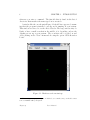
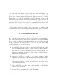
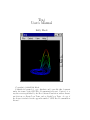
Traj
User’s Manual
Kelly Black
Copyright (c) 2004 Kelly Black
Permission is granted to copy, distribute and/or modify this document
under the terms of the GNU Free Documentation License, Version 1.2 or
any later version published by the Free Software Foundation; with no Invariant Sections, no Front-Cover Texts, and no Back-Cover Texts. A copy of
the license is included in the appendix entitled ”GNU Free Documentation
License”.
2
Trajectory
User’s Manual
Contents
1 Introduction
1.1 Overview . . . . . . . . . . . . . . . . . . . . . . . . . . . . . .
1.2 The Interface . . . . . . . . . . . . . . . . . . . . . . . . . . .
1.3 Differential Equations . . . . . . . . . . . . . . . . . . . . . . .
2 The
2.1
2.2
2.3
2.4
2.5
2.6
File Menu
Introduction . . . . . . . . . . . . . . .
Clearing the Window . . . . . . . . . .
Data File . . . . . . . . . . . . . . . .
Importing Data . . . . . . . . . . . . .
2.4.1 Reading the data file circle.dat
2.4.2 Reading the data file lorenz.dat
2.4.3 Data File Format . . . . . . . .
Equations . . . . . . . . . . . . . . . .
Quitting . . . . . . . . . . . . . . . . .
.
.
.
.
.
.
.
.
.
.
.
.
.
.
.
.
.
.
.
.
.
.
.
.
.
.
.
.
.
.
.
.
.
.
.
.
.
.
.
.
.
.
.
.
.
.
.
.
.
.
.
.
.
.
.
.
.
.
.
.
.
.
.
.
.
.
.
.
.
.
.
.
.
.
.
.
.
.
.
.
.
.
.
.
.
.
.
.
.
.
.
.
.
.
.
.
.
.
.
.
.
.
.
.
.
.
.
.
.
.
.
.
.
.
.
.
.
5
5
5
7
11
11
11
11
12
12
14
16
17
18
3 The
3.1
3.2
3.3
Equation Window
21
Entering An Equation . . . . . . . . . . . . . . . . . . . . . . 22
Saving and Recalling Equations . . . . . . . . . . . . . . . . . 25
Operations and Functions . . . . . . . . . . . . . . . . . . . . 25
4 The
4.1
4.2
4.3
4.4
4.5
4.6
Select Menu
Introduction . . . . . . . . . . . . . . .
Using the Tab Key to Make Selections
Selecting All of the functions . . . . . .
Stepping Through the Functions . . . .
Deselecting all of the Functions . . . .
Deleting functions . . . . . . . . . . . .
3
.
.
.
.
.
.
.
.
.
.
.
.
.
.
.
.
.
.
.
.
.
.
.
.
.
.
.
.
.
.
.
.
.
.
.
.
.
.
.
.
.
.
.
.
.
.
.
.
.
.
.
.
.
.
.
.
.
.
.
.
.
.
.
.
.
.
.
.
.
.
.
.
.
.
.
.
.
.
29
29
29
31
31
32
32
4
5 The
5.1
5.2
5.3
5.4
5.5
5.6
CONTENTS
View Menu
Introduction . . . . .
Show Rotation Point
Toggle Background .
Color . . . . . . . . .
Format . . . . . . . .
Axis . . . . . . . . .
.
.
.
.
.
.
.
.
.
.
.
.
.
.
.
.
.
.
.
.
.
.
.
.
.
.
.
.
.
.
.
.
.
.
.
.
33
33
33
33
34
34
34
A GNU Free Documentation License
1. APPLICABILITY AND DEFINITIONS . . . . . . . . .
2. VERBATIM COPYING . . . . . . . . . . . . . . . . .
3. COPYING IN QUANTITY . . . . . . . . . . . . . . . .
4. MODIFICATIONS . . . . . . . . . . . . . . . . . . . .
5. COMBINING DOCUMENTS . . . . . . . . . . . . . .
6. COLLECTIONS OF DOCUMENTS . . . . . . . . . . .
7. AGGREGATION WITH INDEPENDENT WORKS . .
8. TRANSLATION . . . . . . . . . . . . . . . . . . . . . .
9. TERMINATION . . . . . . . . . . . . . . . . . . . . . .
10. FUTURE REVISIONS OF THIS LICENSE . . . . . .
ADDENDUM: How to use this License for your documents
.
.
.
.
.
.
.
.
.
.
.
.
.
.
.
.
.
.
.
.
.
.
.
.
.
.
.
.
.
.
.
.
.
.
.
.
.
.
.
.
.
.
.
.
.
.
.
.
.
.
.
.
.
.
.
43
44
46
46
47
49
50
50
51
51
51
52
.
.
.
.
.
.
.
.
.
.
.
.
.
.
.
.
.
.
.
.
.
.
.
.
.
.
.
.
.
.
.
.
.
.
.
.
.
.
.
.
.
.
.
.
.
.
.
.
.
.
.
.
.
.
.
.
.
.
.
.
.
.
.
.
.
.
.
.
.
.
.
.
.
.
.
.
.
.
.
.
.
.
.
.
.
.
.
.
.
.
.
.
.
.
.
.
.
.
.
.
.
.
Bibliography
53
Index
54
Trajectory
User’s Manual
Chapter 1
Introduction
1.1 Overview The program, traj, was written to help students visualize
the solution to systems of ordinary differential equations (ODEs). It allows
you to read a data file or specify a system of equations which can be approximated using several different numerical techniques. The program allows you
to view the solution in 3D space, and you can choose the phase space yourself.
This manual is designed to offer an overview of how to use the program
and is not designed to be an introduction to ODEs. It is assumed that you
have some basic knowledge of ODEs. The program was designed for students
learning the topic, however, so the examples are relatively straight-forward
and some background info is included.
The organization of this manual is not intuitive if you are focused on the
ODEs. It is designed to offer a reference for using the program. I have chosen
to organize this manual in terms of the program interface. Hopefully, this
will make it easier to find information while you are using the program. It
is probably quite maddening if you are reading this manual hoping to learn
about the equations themselves.
1.2 The Interface The name of the program is called “traj”. To start
the program from the command line in linux simply type in the name of the
program:
[user]$ traj
If the program does not start make sure that it is installed and that the
program is in your path. The “path” is a list of directories that are searched
5
6
CHAPTER 1. INTRODUCTION
whenever you enter a command. The first file that is found in the list of
directories that matches the name typed in is executed.1
A window like the one shown in Figure 1.1 should have appeared, assuming that the program is installed correctly and is running on your system.
This window is refereed to as the Main Window The large window may be
blank or have a small cross-hair in the middle of it depending on how the
defaults are set up on your system. The cross-hair can be toggled on and
off by clicking on the “View” menu and choosing the option “Show Rotation
Point.”
Figure 1.1: Blank screen from start-up.
1
This is an operating system question. If this does not make sense you should contact
someone familiar with your system.
Trajectory
User’s Manual
1.3. DIFFERENTIAL EQUATIONS
7
Across the top of the window is the main menu. By moving your mouse
over the different items in the main window and clicking the left button more
menus “drop down” and can be seen. Clicking on the items in the drop down
menus allows you to choose the various options described in this manual. It
is assumed that you are familiar with using the mouse to choose the different
menus, and the options themselves will be the main topic of this document.
Directly below the main menu is the viewing window. This is where
the solutions to the differential equations will appear. The different menu
options will allow you to change how the solutions appear. A number of other
keys allow you to rotate and move the solutions in the window. To rotate
an object in the viewing window move the mouse cursor into the viewing
window, press and hold the left button down, and move the cursor. To
move an object (this will be called “translate” here) move the mouse cursor
into the viewing window, press and hold the middle button down, and move
the cursor.
On the far right of the window there is a set of buttons used to control how
objects are viewed in the main window. The button in the middle (marked
with a “c”) is used to center the objects in the window. For example, if you
move the cross-hair away from the center using the middle mouse button,
you can press the “c” button, and it will be automatically centered in the
viewing window.
The top button is used to zoom in on the object in the window, and
the bottom button is used to zoom out. Pressing the “+” button makes
things look bigger, and pressing the “-” button makes things look smaller.
These buttons will not do anything unless some object is in the window. The
rotation point is not considered to be an object. It is simply a reference point
and always looks the same size no matter how you zoom in and out on the
window.
1.3 Differential Equations Differential equations are an important tool.
They use used to develop mathematical models to describe physical phenomena. In many physical systems we do not know the equation describing the
physical quantity we are interested in, but by applying a physical principle
a relationship that includes the physical quantity and its rate of change can
be found.
For example, if we are interested in finding the position of some object we
probably do not know in advance what its location is. Otherwise, there would
not be any problem! To find the position we have to apply some physical
Trajectory
User’s Manual
8
CHAPTER 1. INTRODUCTION
principle and try to work the resulting equation backward. For the movement
of objects we often apply Newton’s Second Law which states that the mass
times the acceleration of an object is equal to the sum of all of the forces on
the object. Another way to state Newton’s Second Law is that momentum
is conserved. The momentum of some object does not change unless a force
is applied. (This focus on momentum is one of the great break-throughs in
modern science.[3])
It turns out that the acceleration, velocity, and position of an object are all
related. The way we express this relationship mathematically is through the
derivative, or instantaneous rate of change. The acceleration is the derivative
of the velocity, and the velocity is the derivative of the position. For more
information on how this relationship is derived see the books by Ostebee and
Zorn[2], Hughes-Hallet and Gleason[1], or any other text book.
An example of an ODE is the equation
d
y(t) = y(t),
dt
y(0) = y0 .
(1.1)
The equation is called an ordinary differential equation because it has a
derivative in it. The word ordinary is used because the function only depends
on one variable, t. In higher dimensions the word “ordinary” is replaced by
the word “partial.” We will only look at ODEs.
Given Equation (1.1) the goal is to figure out what the unknown function,
y(t), is. It turns out we also need to know at least one more thing about the
function. In equation (1.1) we are given an initial condition which is specified
in the second line. Equation (1.1) is usually examined because it is has the
least amount of notation possible, and it can be solved. In fact it is one of
the few equations that we can actually solve.2
Unfortunately, most ODEs that arise in the real world are far more complex than the one given in equation (1.1). In fact, the vast majority of ODEs
do not have known closed form solutions (This means we do not yet know
how to find an expression for the solution in convenient terms.) One way
around this problem is to use the computer to build an approximation to
2
One of the dirty little secrets of the mathematics department is that there are relatively
few ODEs that can be solved analytically. The vast majority of the equations that we can
solve analytically are those found in the ODE class given at most colleges. This leads far
too many students to think that mathematics is just a bunch of techniques and most of it
is known. Nothing could be further from the truth.
Trajectory
User’s Manual
1.3. DIFFERENTIAL EQUATIONS
9
the solution. There are many different ways to construct an approximation.
Each method has its own advantages and disadvantages. The program traj
has three different methods built in, a fourth order Runge-Kutta method, a
Runge-Kutta-Fehlberg method, and Euler’s method.
The fourth order Runge-Kutta (RK4) method is a good general purpose
scheme for building an approximation. The Runge-Kutta-Fehlberg (RKF)
method is based on the RK4 method, but it is an “adaptive” method. It
changes the way it steps in time if the function appears to show some wide
variations. Euler’s method gives an awful approximation. The only reason it
is included is because it is easiest to explain, and many teachers like to have
it included so that it can be used as a learning tool.
The important thing to keep in mind here is that there are three things.
There is a physical system. The physical system is described using a mathematical model. Often times the mathematical model is approximated using
some sort of numerical scheme. You should always keep this in mind. Some
times the mathematical model is not very good so it does not matter how
good the numerical approximation is. Some times the mathematical model
is good, but the numerical scheme is not very good. To be useful all the steps
have to be good.3
3
The definition of the word “good” is something that both scientists and mathematicians have to agree on. It is best left for more advanced studies.
Trajectory
User’s Manual
10
Trajectory
CHAPTER 1. INTRODUCTION
User’s Manual
Chapter 2
The File Menu
2.1 Introduction The file menu contains the options that allow you clear
the viewing window, to add new approximations, print, and to quit the
program. Each of the options is described in separate sections. The options
to clear the window and to quit are relatively straightforward.
You should be very careful about choosing the quit button. At present,
the application quits and does not ask for confirmation. It is possible to lose
your work if you are not careful.
2.2 Clearing the Window The program allows you to display the approximation to more than one equation at a time. You can clear the viewport
of all of the approximations by choosing the “Clear Plot” option from within
the File menu. A window will pop up asking if are sure. If you click the
button that says “yes” the whole window will be cleared. If you click the
button that says “no” then no action will take place.
2.3 Data File There are two ways to get a solution or an approximation
into the viewing window. One way is to read a text file that contains the
numbers representing the approximation. The other way is to enter in the
equations and let the program construct an approximation. The program
can read in the data much quicker than it can produce an approximation. It
can be more troublesome to generate the data using another program and
save the data.
In some circumstances the data files either already exist or someone created a file for a specific purpose. In either case, the program has the ability
to import a file. The way to import a file will be briefly described, and the
11
12
CHAPTER 2. THE FILE MENU
format of the file will then be discussed.
2.4 Importing Data To read a file choose the option “Add from data
file” from the file menu. A window should immediately pop up. You need to
enter a file name in the box. (You can also choose a file using a “point-andclick” on the file name displayed in the window.)
There should be three examples installed on your system. If you do not
know where the traj package was installed you should ask the person who
installed it on your system. There should be a subdirectory called “examples”
in the directory where traj was installed. There are three files that can be
imported, circle.dat, lorenz.dat, and six.dat.
The file circle.dat contains the solution that looks like a spiral. The file
lorenz.dat contains an approximation to a system of ODEs that gives the
“Lorenz Attractor.” The file six.dat contains the Lorenz Attractor as well as
the Butterfly Attractor. It is used for as example in the section that describes
how to change the axis (page 34).
2.4.1 Reading the data file circle.dat The first example focuses on
the function defined in the data file circle.dat. This function defines a spiral
and has three parts. The domain is the times from zero to ten. As the time
increases the other two parts define a circle of radius one.
The three parts can be plotted as a three-dimensional figure using an x, a
y, and a z-axis. The data file has been created so that the times are initially
plotted on the z-axis. (The format of the data file is described on page 16,
and the options for changing the axes is described on page 34.) The other
two parts are initially plotted on the x and y axes.
The first step to read the data file and plot it is to choose “Add from
data file” from the File menu. When this option is chosen a window should
appear asking for a file name, see Figure 2.1. (It is assumed that you are
familiar with the idea of directories and how to use a file dialog box.) Find
the directory where the example files are installed on your system (you will
have to ask the person who installed the files) and choose the file called
“circle.dat.”
Assuming that you can find the file and it has not been corrupted then
you should see the image shown in Figure 2.2. This is a head on view of the
function. The time axis is pointing straight out of the window and cannot
be seen. The effect is that it looks like a two-dimensional plot of a circle.
To view how the whole function appears you have to rotate the view. To
Trajectory
User’s Manual
2.4. IMPORTING DATA
13
Figure 2.1: Importing the file circle.dat.
do this move the mouse pointer over the viewing window. Press and hold
down the far left button on your mouse and then move the mouse. (This is a
long winded way to say click and drag the pointer across the window.) You
should be able to see the view change as you drag the pointer around the
window.
The images in Figures 2.3 through 2.5 show different views of the function.
It is difficult to visualize what the function looks like from looking at just
one view. The program allows you to move and examine the function from
a wide variety of view points. Given a function, you should rotate and view
the function from all possible angles.
You can move (translate) the whole function by dragging the mouse with
the middle button held down. It works the same way as the rotations described above. The difference is that the whole image moves up and down
as well as left and right. Notice that if you translate the image the rotations
appear to be different. The rotations always occur with respect to the center
of the window.
Trajectory
User’s Manual
14
CHAPTER 2. THE FILE MENU
Figure 2.2: Initial view of the function defined in circle.dat.
If you want to center the object in the window click on the button marked
“c” on the far right of the window. This will reset the view to the same as
it was when you first read in the file. This allows you to make whatever
changes you want and easily reset the view.
2.4.2 Reading the data file lorenz.dat There is another example file
included with the program called lorenz.dat. If you import the file in the
same way described in the previous subsection you should see the top of
the Lorenz attractor (see Figure 2.6). This is an approximation to a well
known equation, but the specifics are not discussed here. Try reading both
the circle.dat file and the lorenz.dat file to see what it looks like to have two
approximations at once.
If you import the file after reading circle.dat and you look real closely
Trajectory
User’s Manual
2.4. IMPORTING DATA
15
Figure 2.3: View of the function defined in circle.dat after a small rotation.
you should see that the function defined in circle.dat is still in the picture as
well. A better view of the attractor can be seen by rotating the picture (see
Figure 2.7) and viewing it from different angles. The different views should
make it easier to see the much smaller spiral in the center of the other plot.
If you are feeling particularly adventurous try hitting the “tab” key several times. Each time you hit the key a box should appear around the
different plots. (I am assuming that you have loaded both circle.dat and
lorenz.dat.) This is the selector box and is used to let you know which approximation is “selected.” You can change the way the selected function is
plotted. There is more information on how to use the select feature on page
29 and more information on what to do with a selected function throughout
this manual but especially in the chapter on the View menu option, Chapter
5.
Trajectory
User’s Manual
16
CHAPTER 2. THE FILE MENU
Figure 2.4: View of the function defined in circle.dat after another small
rotation.
You can also delete a selected function. To delete a function first select
and then hit the “delete” key. Be careful about this because there is no
warning. Unlike the clear plot option the function is simply deleted with
little fanfare.
2.4.3 Data File Format The data file is kept as simple as possible. Each
row should contain the same number of points as the dimension number, and
the number of rows is equal to the number points you want to plot. For
example, the function defined in the file circle.dat has three dimensions.
There are also a large number of points used to describe the function. Each
row in the data file has three numbers, one for each dimension, and each data
point is in a separate row.
Trajectory
User’s Manual
2.5. EQUATIONS
17
Figure 2.5: View of the function defined in circle.dat after yet another small
rotation.
The first four lines and last three lines are shown in Table 2.1. (The file
was created using matlab and saving the array in ASCII format.) The first
row defines the first data point, (1,0,0). The second row defines the second
data point. The last line defines the last data point that will be plotted.
The way the data file was created the first two dimension are data points
describing a circle in two dimensions. The third dimension (given in the third
column) can be thought of as the time and is equally spaced, each time step
is 0.05 in whatever units you happen to be using.
2.5 Equations Choosing the option “Add from equation” from the File
menu brings up the equation window. This window has the most options
and is examined in its own chapter, Chapter 3. If you want to look at some
Trajectory
User’s Manual
18
CHAPTER 2. THE FILE MENU
Figure 2.6: Initial view of the functions in circle.dat and lorenz.dat.
examples, read in some of the example equation files.
These files have the extension .eqn and should be installed in the example
directory. If you do not know where this directory is ask the person who
installed the package. The example subdirectory should be in the directory
where the package was originally installed but may have been moved by the
person who installed the package.
2.6 Quitting To quit choose the “quit” option from the file menu. Be
careful about doing this. No confirmation message will be displayed. The
program will simply exit with no fanfare what so ever.
Trajectory
User’s Manual
2.6. QUITTING
19
Figure 2.7: Rotated view of the functions in circle.dat and lorenz.dat.
1.0000000e+00 0.0000000e+00
9.9875026e-01 4.9979169e-02
9.9500417e-01 9.9833417e-02
9.8877108e-01 1.4943813e-01
..
..
.
.
-8.8919115e-01 -4.5753589e-01
-8.6521263e-01 -5.0140513e-01
-8.3907153e-01 -5.4402111e-01
0.0000000e+00
5.0000000e-02
1.0000000e-01
1.5000000e-01
..
.
9.9000000e+00
9.9500000e+00
1.0000000e+01
Table 2.1: First four lines and last three lines of the file circle.dat
Trajectory
User’s Manual
20
Trajectory
CHAPTER 2. THE FILE MENU
User’s Manual
Chapter 3
The Equation Window
The two ways to obtain equations to plot is to read a data file or to specify
a system of differential equations. Here we focus on how to specify a system
of differential equations. A system of equations can be entered through the
Equation Entry window. This window is created when you choose “File”
from the main window and then choose “Add From Equation.” The window
that appears is shown in Figure 3.1.
The labels for each function in the system of equations are assumed to
be of the form y01 (t), y02 (t), y03 (t) up to y08 (t). Once a system of equations
is specified the program will approximate the system using one of the built
in solvers. A system is specified once the following is provided:
• The number of equations in the system,
• The differential equation for each function,
• The initial condition for each function,
• The start time,
• The end time,
• The time step to be used for the solver.
Once each of these items is provided the program will display an approximation once the Plot button is clicked.
21
22
CHAPTER 3. THE EQUATION WINDOW
Figure 3.1: Equation window with no equations.
3.1 Entering An Equation To enter a system of equations you need to
first specify the number of equations in the system. This number is specified
at the top left text box in the equation window. Once this number is specified
you must then enter each differential equation in the entries below. The
dependent variables are labeled from y01 (t) to y08 (t), and the independent
variable is assumed to be time, t. For each of these functions a differential
equation must be specified.
A number of standard functions are recognized and are listed in subsection
3.3. A function is composed of constants, the independent variable, the
independent variables, the basic operations and pre-defined functions listed in
subsection 3.3. The basic operations include addition, subtraction (including
unary minus), multiplication, division, and exponentiation. The symbol used
for exponentiation is “ ˆ ”. (Some examples will be given below.) The order
of operations is the usual convention, and parenthesis can be used to group
operations.
When typing in an equation the independent variables are referred to as
Trajectory
User’s Manual
3.1. ENTERING AN EQUATION
23
“Y01,” “Y02”, through “Y08”. The variables do not have to be typed in
upper case and the “0” is optional. For example to refer to the function
y04 (t) you could also type either “y08” or “y8.” The independent variable is
typed as “t” or “T.” Constants are typed as a string of numbers.
Once the equations for each dependent variable are entered an initial
condition for each variable must be specified. This is a number which specifies the value of the dependent variable at the initial time. The initial (or
starting) time and the end time is specified at the end of the list of equations. Additionally, an initial time step must be specified which is used by
the numerical approximation that is chosen.
Once all of these things are entered a plot of the approximation is displayed once the “plot” button is clicked.
As an example we examine two different systems of equations. The first
is a simpler, linear problem
d
y01 (t) = −y02 (t),
dt
d
y02 (t) = y01 (t),
dt
(3.1a)
(3.1b)
where the intial conditions are
y01 (0) = 1,
y02 (0) = 1.
(3.2a)
(3.2b)
Here we will plot the equation for time between 0 and 100 with an initial
time step of 0.1. (A list of the available approximation schemes is given on
page 9.) The solution to this equation is a circle in phase space. This system
of equations entered in the equation window is shown in Figure 3.2.
First, the number of dependent variables must be specified. In this case
we have a system of two equations so at the top left of the window a “2” is
entered next to the text “N=.” Next the two equations must be entered. In
particular, the first equation,
d
y01 (t) = −y02 (t),
dt
is entered as
-y2.
Trajectory
User’s Manual
24
CHAPTER 3. THE EQUATION WINDOW
Figure 3.2: Equation window with two dimensional ODE that results in a
circle in the phase space.
The second equation,
d
y02 (t) = y01 (t),
dt
is entered as
y1.
To the right of each equation, the initial condition for the coresponding
dependent variable is specified. Finally, the initial time, the end time, and
the time step must be specified. Here the initial time is set to 0 and the final
time is set to 100. The time step is set to 0.1. Once these numbers and the
equations are set a plot can be displayed by clicking on the “Plot” button.
When the button is clicked an approximation to the equation is found and
then plotted. The method used to construct the approximation is specified in
the “Integration” menu. To check or set the approximation method click on
Trajectory
User’s Manual
3.2. SAVING AND RECALLING EQUATIONS
25
the “Integration” menu at the top of the window. The current approximation
method is marked. To change the approximation method choose a different option from the menu. The default method is a Runge-Kutta-Fehlberg
method using a fourth order approximation with a fifth order check.
The second example demonstrates the Lorenz equation,
d
y01 (t) = −12(y01 − y02 ),
dt
d
y02 (t) = 28y01 − y02 − y01 y03 ,
dt
d
y03 (t) = 2.7(y01 y02 − y03 ).
dt
(3.3a)
(3.3b)
(3.3c)
Here we use the initial condition
y01 (0) = 3,
y02 (0) = 4,
y03 (0) = 18.
(3.4a)
(3.4b)
(3.4c)
The way to enter this equation is shown in Figure 3.3. Once the equations,
the initial conditions, and the times are specified you can click on the “plot”
button, and an approximation is found and plotted.
3.2 Saving and Recalling Equations Once a set of equations are entered they can be saved and recalled for later use. To save a set set of equations clicke on the “File” menu and choose “Save.” You will be prompted to
supply a file name. It is assumed that the file will end with an “.eqn.” You
can then recall the file by clicking on the “File” menu and choosing “Open.”
You must then specify the file name of a previously saved set of equations.
3.3 Operations and Functions The following functions are recognized
within an equation entry:
+ The sum of two numbers. (Unary plus is not supported.)
Example: y1 + 5.
- Either the difference of two numbers are the negative of a given number.
(Unary minus is supported.)
Example: y2 − 8 or −y3 + t.
Trajectory
User’s Manual
26
CHAPTER 3. THE EQUATION WINDOW
Figure 3.3: Equation window with the system of equations for the Lorenz
equation.
* The product of two numbers.
Example: y1 ∗ y3.
/ The quotient of two numbers.
Example: y2/8.
ˆ Exponentiation of two numbers.
Example: 12.5/y1.
( Left parenthesis.
) Right parenthesis.
Example: (y1 − t)/y4 ˆ (1/3).
ln Natural Logarithm. The argument must be enclosed in parenthesis.
Example: ln(y1 + 4).
Trajectory
User’s Manual
3.3. OPERATIONS AND FUNCTIONS
27
exp Exponential. The argument must be enclosed in parenthesis.
Example: exp(y2 − 4).
sin Sine. The argument must be enclosed in parenthesis.
Example: sin(t + y6).
cos Cosine. The argument must be enclosed in parenthesis.
Example: cos(y1 + y2 − t).
tan Tangent. The argument must be enclosed in parenthesis.
Example: tan(t/y2).
asin Inverse Sine (arcsine). The argument must be enclosed in parenthesis.
Example: asin(y3).
acos Inverse Cosine (arccosine). The argument must be enclosed in parenthesis.
Example: acos(t/y1 + 1).
atan Inverse Tangent (arctangent). The argument must be enclosed in
parenthesis.
Example: atan(y1/y4).
abs Absolute Value. The argument must be enclosed in parenthesis.
Example: abs(y2).
sqrt Square Root. The argument must be enclosed in parenthesis.
Example: sqrt(y12 + 1).
floor Floor. (The largest integer that is smaller than the argument passed.)
The argument must be enclosed in parenthesis.
Example: floor(y1/y2).
ceil Ceiling. (The smallest integer that is bigger than the argument passed.)
The argument must be enclosed in parenthesis.
Example: ceil(y13 ).
trunc Truncation (Remove the fraction from the argument passed.) The
argument must be enclosed in parenthesis.
Example: trunc(y3 − y2).
Trajectory
User’s Manual
28
Trajectory
CHAPTER 3. THE EQUATION WINDOW
User’s Manual
Chapter 4
The Select Menu
4.1 Introduction There are many ways to change the way a function
is viewed. The different options are discussed throughout this manual and
especially in chapter 5. You can change the options on all of the functions or
on individual functions that are in the current viewport. In order to change
the options for a particular function you must first select it, and there are a
couple of different ways to do this. If no functions are selected and an option
is changed, the change will effect all of the functions being viewed.
For all of the examples here it is assumed that you have at least two
functions plotted in the main viewing window. In particular the figures
given will use the two functions defined by the example data files lorenz.dat
and circle.dat. Information on how to import the two files is given on page
12 and page 14.
The different ways to select an object include using the “tab” key to select
one function at a time. Using the options from within the Select option on
the main menu you can select all of the functions, step through the functions,
or turn off all of your selections. Each of these different options is discussed
in the sections that follow.
4.2 Using the Tab Key to Make Selections The program keeps track
of the functions that you add to the viewport and keeps them in a list. You
can select one function at a time and step through each function by hitting
the “tab” key. Each time you hit the tab key it will turn off the current
selection, move to the next function in the list, and select it. When a function
is selected a box around the function is drawn.
In Figures 4.1 and 4.2 the sequence is shown. In this particular example,
29
30
CHAPTER 4. THE SELECT MENU
Figure 4.1: The spiral is selected and the Lorenz attractor is not selected.
the Lorenz attractor was imported first followed by the spiral. The first time
the tab key is struck the spiral is selected. (The list is kept in reverse order.)
This is shown in Figure 4.1. The second time the tab key is struck the
selection box moves from the spiral to the Lorenz attractor. This is shown
in Figure 4.2.
Once you have stepped through and have chosen each of the functions the
next time you hit the tab key then no selection is made. In this example, the
third time you hit the tab key no selection is in effect. To start the selection
sequence again you have to hit tab again, and the whole process begins anew.
Be careful about hitting the delete key while any of the functions are
selected. A selected function will be deleted. The program will not ask for
confirmation; it will just delete the function.
Trajectory
User’s Manual
4.3. SELECTING ALL OF THE FUNCTIONS
31
Figure 4.2: The spiral is not selected and the Lorenz attractor is selected.
4.3 Selecting All of the functions You do not have to select only one
function at a time. It is possible to select all of the functions at one time.
To do this choose the option “Select All” from the Select menu. This will
select all of the functions in the viewport, and a box will be drawn around
each function. An example of this is shown in Figure 4.3.
4.4 Stepping Through the Functions Another way to step through
and select one function at a time is using the “Select Next” option in the
Select menu. This works exactly like the tab key as discussed in section 4.2.
This option is in place in case the tab key does not work on your system or
you are more comfortable using the menu.
Trajectory
User’s Manual
32
CHAPTER 4. THE SELECT MENU
Figure 4.3: Both the spiral is selected and the Lorenz attractor is selected.
4.5 Deselecting all of the Functions If you would like to turn off all
of the selections choose the “Deselect All” option from the Select menu. This
simply turns off all of the selections, and all of the bounding boxes are turned
off.
4.6 Deleting functions There are two different ways to delete functions.
To delete a specific function you simply select it and hit the delete key. The
function will be deleted, but the program will not ask for confirmation. It is
assumed that when you hit the delete key you really mean it.
The other way to delete functions is to clear the whole menu. To do
this choose “Clear Plot” from the File menu. You will be given a chance to
confirm your decision. If you answer yes in the box that pops up all of the
functions will be deleted.
Trajectory
User’s Manual
Chapter 5
The View Menu
5.1 Introduction You can change the way you view a function. For
example, the function can be plotted using different color schemes and different values can be plotted on different axes. The program allows you to
make changes to one function or all of the functions. If a function is selected
and changes to the view only affect the function selected. If no functions are
selected then any change affects all of the functions.
The things that you can change include whether or not the cross-hairs are
displayed. It also includes the background color as well as the color scheme
used to generate the plot. You can also toggle between plotting a function
using dots at the data points or lines connecting the data points. Finally,
you can change which variable is plotted on the x, y, and z-axis.
5.2 Show Rotation Point The rotation point is misnamed and is an
artifact of a lack of imagination of the programmer. The rotations take place
relative to the center of the viewing window. The cross-hair that is displayed
simply shows the center of all of the functions.
You can turn this off or on depending on what you think looks best. To
do this select the option “Show Rotation Point” from the View menu. The
cross-hair will be toggled on and off as you choose this option.
5.3 Toggle Background The color of the background can be toggled
between white and black. Printing the plot prints the background in the
color on the screen. If you are printing onto a sheet of paper it may be best
to use a white background.
To toggle back and forth between the two colors choose the “Toggle Back33
34
CHAPTER 5. THE VIEW MENU
ground” from the View menu.
5.4 Color Another option is to change the way that the color is applied
to the function. All of the examples that we have seen have applied the color
with respect to the z-coordinate. The part of a function with the lowest
z-value are red while the parts with the largest value on the z-axis are blue.
The colors in between range from red to green to blue.
There are two other options. You can color the function in the order that
the data points are generated, or you can color the function in a single color
(black or white). To color the function in order first click on the View menu
and click on the color option. In the menu that drops down choose “Color
by Order.” An example of what the Lorenz attractor looks like is shown in
Figure 5.1.
This is not a very good example, but there are times when you are not
sure where the function starts and ends. When the function is colored by
order the first numbers are colored red, and the last numbers are colored
blue. The numbers in the middle go from red to green to blue.
If you choose the option “Single Color” the function is plotted in either
black or white. If the background is white the function is plotted in black,
otherwise the background is black and the function is white. This option is
provided in case you want to print the viewport in black and white.
5.5 Format Another option for the way a function can be plotted is
whether or not each data point is plotted as a point in space or the data
points are connected. Usually it is more convenient to examine the data
points connected. So far all of the examples seen have been for connected
points. If you are viewing data generated from difference equations or there
are an extremely large number of points then it may be better to view the
plot as a collection of plots.
To choose between the two options click on the View menu and click on
“Format.” There are two options. If you click on “Draw Points” then points
will be drawn. If you choose “Draw Lines” then lines connecting the data
points will be drawn. All of the figure shown so far have been drawn using
lines. The plot in Figure 5.2 is the Lorenz attractor drawn using the points.
5.6 Axis The program allows you to look at the data in different ways.
The most useful feature is that it allows you to look at the data along different axis. Unfortunately, we are three-dimensional animals, and we cannot
Trajectory
User’s Manual
5.6. AXIS
35
Figure 5.1: The Lorenz attractor plotted by coloring the points in the order
that they were originally generated.
visualize beyond three dimensions without a whole lot of meditation (and
probably a couple of medications).
The solutions to systems of ODEs represent the values of a number of
functions. The domain of the functions is some specific time interval. It is
useful to look at each function by itself as a function of time. At the same
time, there is no law that says we have to view each of these functions by
themselves. We can also plot them against each other to see how they are
related.
Each function is represented on the computer as a list of numbers. For a
system of equations the computer stores the same number of points for each
function. Given a list of three functions we get three lists of numbers. The
values of the functions at a specific time is stored as three numbers. We can
Trajectory
User’s Manual
36
CHAPTER 5. THE VIEW MENU
Figure 5.2: The Lorenz Attractor from lorenz.dat plotted using points.
treat those three numbers as a point in three-dimensional space. This is the
basic idea behind the “phase space.”
Given a list of functions we pick any three of the functions and treat the
functions as points in three-dimensional space. The program allows you to
choose whichever functions you would like and plot them along whichever
axis you would like to see. As you change which function is plotted along
which axis you can view the different phase portraits of the function.
As an example, there is a data file called six.dat included in the examples.
If you do not know where the file is located ask the person who installed the
package on your system. The file should be located in the subdirectory
called examples. The file has six different functions within it. The first three
functions are an approximation that gives the Lorenz attractor. The next
three functions are an approximation of a set of equations that gives what is
Trajectory
User’s Manual
5.6. AXIS
37
called the “Butterfly Attractor.”
In this example, clear all of the plots and import the file six.dat. The
approximation that was made generated an extremely large number of points.
The resulting plot does not look very good. It looks a little bit better plotting
in points mode (see Section 5.5). A view of the function is shown in Figure
5.3.
Figure 5.3: The Lorenz attractor plotted using points. Data file is from
six.dat
The first three functions are approximations of the Lorenz attractor. If
you want to see what the other functions look like you need to change which
functions are plotted on the x, y, and z-axes. Each axis will have to be defined
separately. The windows that are used to do this are shown in Figures 5.4
through 5.6.
Trajectory
User’s Manual
38
CHAPTER 5. THE VIEW MENU
First, to choose to reset the x-axis click on the View Menu and click
on “Axis.” In the menu that appears click on “Set X-Axis.” The window
shown in Figure 5.4 should appear. The functions in the file have to be
labeled in some manner. The convention is that the first column is called
“Time”, and the rest of the functions are numbered starting at zero. The six
functions that are found in the file six.dat are named in the following way:
the first function (column one) is called the variable “Time.” (This is just a
convention and not always followed.) The second function (column two) is
called the variable y00. The third function (column 3) is called the variable
y01. The final function (column 6) is called the variable y04.
Figure 5.4: Choose the X-axis to be y02.
To view the butterfly attractor first set the x-axis to be plotted using
the variable y02. Then set the y-axis to be plotted using the variable y03,
and finally set the z-axis to be plotted using the variable y04. The steps to
do this are shown in Figures 5.4 through 5.6. Note that as you do this the
intermediate plots are incoherent.
Sometimes this happens. Often times you have to look at the different
Trajectory
User’s Manual
5.6. AXIS
39
Figure 5.5: Choose the Y-axis to be y03.
phase portraits until you find something that displays a pattern. That is
why this program was written. It allows you to search through the different
phase portraits to try to find any patterns that might be hidden in the data.
Note that in Figure 5.7 if you look at the plot without moving it is extremely
difficult to see any structure in the data. To see the structure you should
view it as a set of points and rotate the plot around to look at it from all
different angles.
Trajectory
User’s Manual
40
CHAPTER 5. THE VIEW MENU
Figure 5.6: Choose the Z-axis to be y04.
Trajectory
User’s Manual
5.6. AXIS
41
Figure 5.7: The Butterfly attractor plotted using points. Data file is from
six.dat
Trajectory
User’s Manual
42
Trajectory
CHAPTER 5. THE VIEW MENU
User’s Manual
Appendix A
GNU Free Documentation
License
The following description of the GNU Free Documentation License was found
at the URL: http://www.gnu.org/licenses/licenses.html#FDL. This is a verbatim copy of the license found on 29 April 2004, and the full text immediately follows.
Version 1.2, November 2002
c
Copyright 2000,2001,2002
Free Software Foundation, Inc.
59 Temple Place, Suite 330, Boston, MA 02111-1307 USA
Everyone is permitted to copy and distribute verbatim copies of this license
document, but changing it is not allowed.
Preamble
The purpose of this License is to make a manual, textbook, or other functional and useful document ”free” in the sense of freedom: to assure everyone
the effective freedom to copy and redistribute it, with or without modifying
it, either commercially or noncommercially. Secondarily, this License preserves for the author and publisher a way to get credit for their work, while
not being considered responsible for modifications made by others.
This License is a kind of ”copyleft”, which means that derivative works
of the document must themselves be free in the same sense. It complements
43
44
APPENDIX A. GNU FREE DOCUMENTATION LICENSE
the GNU General Public License, which is a copyleft license designed for free
software.
We have designed this License in order to use it for manuals for free
software, because free software needs free documentation: a free program
should come with manuals providing the same freedoms that the software
does. But this License is not limited to software manuals; it can be used
for any textual work, regardless of subject matter or whether it is published
as a printed book. We recommend this License principally for works whose
purpose is instruction or reference.
1. APPLICABILITY AND DEFINITIONS
This License applies to any manual or other work, in any medium, that
contains a notice placed by the copyright holder saying it can be distributed
under the terms of this License. Such a notice grants a world-wide, royaltyfree license, unlimited in duration, to use that work under the conditions
stated herein. The ”Document”, below, refers to any such manual or work.
Any member of the public is a licensee, and is addressed as ”you”. You
accept the license if you copy, modify or distribute the work in a way requiring
permission under copyright law.
A ”Modified Version” of the Document means any work containing the
Document or a portion of it, either copied verbatim, or with modifications
and/or translated into another language.
A ”Secondary Section” is a named appendix or a front-matter section
of the Document that deals exclusively with the relationship of the publishers
or authors of the Document to the Document’s overall subject (or to related
matters) and contains nothing that could fall directly within that overall
subject. (Thus, if the Document is in part a textbook of mathematics, a Secondary Section may not explain any mathematics.) The relationship could
be a matter of historical connection with the subject or with related matters,
or of legal, commercial, philosophical, ethical or political position regarding
them.
The ”Invariant Sections” are certain Secondary Sections whose titles
are designated, as being those of Invariant Sections, in the notice that says
that the Document is released under this License. If a section does not fit
the above definition of Secondary then it is not allowed to be designated
as Invariant. The Document may contain zero Invariant Sections. If the
Document does not identify any Invariant Sections then there are none.
Trajectory
User’s Manual
45
The ”Cover Texts” are certain short passages of text that are listed,
as Front-Cover Texts or Back-Cover Texts, in the notice that says that the
Document is released under this License. A Front-Cover Text may be at
most 5 words, and a Back-Cover Text may be at most 25 words.
A ”Transparent” copy of the Document means a machine-readable copy,
represented in a format whose specification is available to the general public,
that is suitable for revising the document straightforwardly with generic text
editors or (for images composed of pixels) generic paint programs or (for
drawings) some widely available drawing editor, and that is suitable for input
to text formatters or for automatic translation to a variety of formats suitable
for input to text formatters. A copy made in an otherwise Transparent file
format whose markup, or absence of markup, has been arranged to thwart or
discourage subsequent modification by readers is not Transparent. An image
format is not Transparent if used for any substantial amount of text. A copy
that is not ”Transparent” is called ”Opaque”.
Examples of suitable formats for Transparent copies include plain ASCII
without markup, Texinfo input format, LaTeX input format, SGML or XML
using a publicly available DTD, and standard-conforming simple HTML,
PostScript or PDF designed for human modification. Examples of transparent image formats include PNG, XCF and JPG. Opaque formats include
proprietary formats that can be read and edited only by proprietary word
processors, SGML or XML for which the DTD and/or processing tools are
not generally available, and the machine-generated HTML, PostScript or
PDF produced by some word processors for output purposes only.
The ”Title Page” means, for a printed book, the title page itself, plus
such following pages as are needed to hold, legibly, the material this License
requires to appear in the title page. For works in formats which do not have
any title page as such, ”Title Page” means the text near the most prominent
appearance of the work’s title, preceding the beginning of the body of the
text.
A section ”Entitled XYZ” means a named subunit of the Document
whose title either is precisely XYZ or contains XYZ in parentheses following text that translates XYZ in another language. (Here XYZ stands for
a specific section name mentioned below, such as ”Acknowledgements”,
”Dedications”, ”Endorsements”, or ”History”.) To ”Preserve the
Title” of such a section when you modify the Document means that it remains a section ”Entitled XYZ” according to this definition.
Trajectory
User’s Manual
46
APPENDIX A. GNU FREE DOCUMENTATION LICENSE
The Document may include Warranty Disclaimers next to the notice
which states that this License applies to the Document. These Warranty
Disclaimers are considered to be included by reference in this License, but
only as regards disclaiming warranties: any other implication that these Warranty Disclaimers may have is void and has no effect on the meaning of this
License.
2. VERBATIM COPYING
You may copy and distribute the Document in any medium, either commercially or noncommercially, provided that this License, the copyright notices, and the license notice saying this License applies to the Document are
reproduced in all copies, and that you add no other conditions whatsoever
to those of this License. You may not use technical measures to obstruct or
control the reading or further copying of the copies you make or distribute.
However, you may accept compensation in exchange for copies. If you distribute a large enough number of copies you must also follow the conditions
in section 3.
You may also lend copies, under the same conditions stated above, and
you may publicly display copies.
3. COPYING IN QUANTITY
If you publish printed copies (or copies in media that commonly have
printed covers) of the Document, numbering more than 100, and the Document’s license notice requires Cover Texts, you must enclose the copies in
covers that carry, clearly and legibly, all these Cover Texts: Front-Cover
Texts on the front cover, and Back-Cover Texts on the back cover. Both
covers must also clearly and legibly identify you as the publisher of these
copies. The front cover must present the full title with all words of the title
equally prominent and visible. You may add other material on the covers in
addition. Copying with changes limited to the covers, as long as they preserve the title of the Document and satisfy these conditions, can be treated
as verbatim copying in other respects.
If the required texts for either cover are too voluminous to fit legibly,
you should put the first ones listed (as many as fit reasonably) on the actual
cover, and continue the rest onto adjacent pages.
If you publish or distribute Opaque copies of the Document numbering more than 100, you must either include a machine-readable Transparent
Trajectory
User’s Manual
47
copy along with each Opaque copy, or state in or with each Opaque copy
a computer-network location from which the general network-using public
has access to download using public-standard network protocols a complete
Transparent copy of the Document, free of added material. If you use the
latter option, you must take reasonably prudent steps, when you begin distribution of Opaque copies in quantity, to ensure that this Transparent copy
will remain thus accessible at the stated location until at least one year after
the last time you distribute an Opaque copy (directly or through your agents
or retailers) of that edition to the public.
It is requested, but not required, that you contact the authors of the
Document well before redistributing any large number of copies, to give them
a chance to provide you with an updated version of the Document.
4. MODIFICATIONS
You may copy and distribute a Modified Version of the Document under
the conditions of sections 2 and 3 above, provided that you release the Modified Version under precisely this License, with the Modified Version filling
the role of the Document, thus licensing distribution and modification of the
Modified Version to whoever possesses a copy of it. In addition, you must
do these things in the Modified Version:
A. Use in the Title Page (and on the covers, if any) a title distinct from that
of the Document, and from those of previous versions (which should, if
there were any, be listed in the History section of the Document). You
may use the same title as a previous version if the original publisher of
that version gives permission.
B. List on the Title Page, as authors, one or more persons or entities
responsible for authorship of the modifications in the Modified Version,
together with at least five of the principal authors of the Document (all
of its principal authors, if it has fewer than five), unless they release
you from this requirement.
C. State on the Title page the name of the publisher of the Modified
Version, as the publisher.
D. Preserve all the copyright notices of the Document.
Trajectory
User’s Manual
48
APPENDIX A. GNU FREE DOCUMENTATION LICENSE
E. Add an appropriate copyright notice for your modifications adjacent to
the other copyright notices.
F. Include, immediately after the copyright notices, a license notice giving
the public permission to use the Modified Version under the terms of
this License, in the form shown in the Addendum below.
G. Preserve in that license notice the full lists of Invariant Sections and
required Cover Texts given in the Document’s license notice.
H. Include an unaltered copy of this License.
I. Preserve the section Entitled ”History”, Preserve its Title, and add to
it an item stating at least the title, year, new authors, and publisher of
the Modified Version as given on the Title Page. If there is no section
Entitled ”History” in the Document, create one stating the title, year,
authors, and publisher of the Document as given on its Title Page, then
add an item describing the Modified Version as stated in the previous
sentence.
J. Preserve the network location, if any, given in the Document for public
access to a Transparent copy of the Document, and likewise the network
locations given in the Document for previous versions it was based on.
These may be placed in the ”History” section. You may omit a network
location for a work that was published at least four years before the
Document itself, or if the original publisher of the version it refers to
gives permission.
K. For any section Entitled ”Acknowledgements” or ”Dedications”, Preserve the Title of the section, and preserve in the section all the substance and tone of each of the contributor acknowledgements and/or
dedications given therein.
L. Preserve all the Invariant Sections of the Document, unaltered in their
text and in their titles. Section numbers or the equivalent are not
considered part of the section titles.
M. Delete any section Entitled ”Endorsements”. Such a section may not
be included in the Modified Version.
Trajectory
User’s Manual
49
N. Do not retitle any existing section to be Entitled ”Endorsements” or
to conflict in title with any Invariant Section.
O. Preserve any Warranty Disclaimers.
If the Modified Version includes new front-matter sections or appendices
that qualify as Secondary Sections and contain no material copied from the
Document, you may at your option designate some or all of these sections
as invariant. To do this, add their titles to the list of Invariant Sections in
the Modified Version’s license notice. These titles must be distinct from any
other section titles.
You may add a section Entitled ”Endorsements”, provided it contains
nothing but endorsements of your Modified Version by various parties–for
example, statements of peer review or that the text has been approved by
an organization as the authoritative definition of a standard.
You may add a passage of up to five words as a Front-Cover Text, and a
passage of up to 25 words as a Back-Cover Text, to the end of the list of Cover
Texts in the Modified Version. Only one passage of Front-Cover Text and
one of Back-Cover Text may be added by (or through arrangements made
by) any one entity. If the Document already includes a cover text for the
same cover, previously added by you or by arrangement made by the same
entity you are acting on behalf of, you may not add another; but you may
replace the old one, on explicit permission from the previous publisher that
added the old one.
The author(s) and publisher(s) of the Document do not by this License
give permission to use their names for publicity for or to assert or imply
endorsement of any Modified Version.
5. COMBINING DOCUMENTS
You may combine the Document with other documents released under
this License, under the terms defined in section 4 above for modified versions,
provided that you include in the combination all of the Invariant Sections
of all of the original documents, unmodified, and list them all as Invariant
Sections of your combined work in its license notice, and that you preserve
all their Warranty Disclaimers.
The combined work need only contain one copy of this License, and multiple identical Invariant Sections may be replaced with a single copy. If there
are multiple Invariant Sections with the same name but different contents,
Trajectory
User’s Manual
50
APPENDIX A. GNU FREE DOCUMENTATION LICENSE
make the title of each such section unique by adding at the end of it, in
parentheses, the name of the original author or publisher of that section if
known, or else a unique number. Make the same adjustment to the section
titles in the list of Invariant Sections in the license notice of the combined
work.
In the combination, you must combine any sections Entitled ”History”
in the various original documents, forming one section Entitled ”History”;
likewise combine any sections Entitled ”Acknowledgements”, and any sections Entitled ”Dedications”. You must delete all sections Entitled ”Endorsements”.
6. COLLECTIONS OF DOCUMENTS
You may make a collection consisting of the Document and other documents released under this License, and replace the individual copies of this
License in the various documents with a single copy that is included in the
collection, provided that you follow the rules of this License for verbatim
copying of each of the documents in all other respects.
You may extract a single document from such a collection, and distribute
it individually under this License, provided you insert a copy of this License
into the extracted document, and follow this License in all other respects
regarding verbatim copying of that document.
7. AGGREGATION WITH
INDEPENDENT WORKS
A compilation of the Document or its derivatives with other separate
and independent documents or works, in or on a volume of a storage or
distribution medium, is called an ”aggregate” if the copyright resulting from
the compilation is not used to limit the legal rights of the compilation’s users
beyond what the individual works permit. When the Document is included in
an aggregate, this License does not apply to the other works in the aggregate
which are not themselves derivative works of the Document.
If the Cover Text requirement of section 3 is applicable to these copies
of the Document, then if the Document is less than one half of the entire
aggregate, the Document’s Cover Texts may be placed on covers that bracket
the Document within the aggregate, or the electronic equivalent of covers if
the Document is in electronic form. Otherwise they must appear on printed
covers that bracket the whole aggregate.
Trajectory
User’s Manual
51
8. TRANSLATION
Translation is considered a kind of modification, so you may distribute
translations of the Document under the terms of section 4. Replacing Invariant Sections with translations requires special permission from their copyright holders, but you may include translations of some or all Invariant Sections in addition to the original versions of these Invariant Sections. You
may include a translation of this License, and all the license notices in the
Document, and any Warranty Disclaimers, provided that you also include
the original English version of this License and the original versions of those
notices and disclaimers. In case of a disagreement between the translation
and the original version of this License or a notice or disclaimer, the original
version will prevail.
If a section in the Document is Entitled ”Acknowledgements”, ”Dedications”, or ”History”, the requirement (section 4) to Preserve its Title (section
1) will typically require changing the actual title.
9. TERMINATION
You may not copy, modify, sublicense, or distribute the Document except
as expressly provided for under this License. Any other attempt to copy,
modify, sublicense or distribute the Document is void, and will automatically
terminate your rights under this License. However, parties who have received
copies, or rights, from you under this License will not have their licenses
terminated so long as such parties remain in full compliance.
10. FUTURE REVISIONS OF THIS
LICENSE
The Free Software Foundation may publish new, revised versions of the
GNU Free Documentation License from time to time. Such new versions will
be similar in spirit to the present version, but may differ in detail to address
new problems or concerns. See http://www.gnu.org/copyleft/.
Each version of the License is given a distinguishing version number. If
the Document specifies that a particular numbered version of this License ”or
any later version” applies to it, you have the option of following the terms
and conditions either of that specified version or of any later version that
has been published (not as a draft) by the Free Software Foundation. If the
Document does not specify a version number of this License, you may choose
any version ever published (not as a draft) by the Free Software Foundation.
Trajectory
User’s Manual
52
APPENDIX A. GNU FREE DOCUMENTATION LICENSE
ADDENDUM: How to use this License for
your documents
To use this License in a document you have written, include a copy of the
License in the document and put the following copyright and license notices
just after the title page:
c
Copyright YEAR
YOUR NAME. Permission is granted to copy,
distribute and/or modify this document under the terms of the
GNU Free Documentation License, Version 1.2 or any later version published by the Free Software Foundation; with no Invariant Sections, no Front-Cover Texts, and no Back-Cover Texts. A
copy of the license is included in the section entitled ”GNU Free
Documentation License”.
If you have Invariant Sections, Front-Cover Texts and Back-Cover Texts,
replace the ”with...Texts.” line with this:
with the Invariant Sections being LIST THEIR TITLES, with the
Front-Cover Texts being LIST, and with the Back-Cover Texts
being LIST.
If you have Invariant Sections without Cover Texts, or some other combination of the three, merge those two alternatives to suit the situation.
If your document contains nontrivial examples of program code, we recommend releasing these examples in parallel under your choice of free software license, such as the GNU General Public License, to permit their use
in free software.
Trajectory
User’s Manual
Bibliography
[1] D. Hughes-Hallet and A. M. Gleason, Calculus, John Wiley &
Sons, Inc., New York, 1 ed., 1994.
[2] A. Ostebee and P. Zorn, Calculus from Graphical, Numerical, and
Symbolic Points of View, vol. 1, Saunders College Publishing, New York,
1 ed., 1997.
[3] R. S. Westfall, Never at Rest, A Biography of Isaac Newton, Cambridge University Press, Cambridge, UK, 1998.
53
Index
Acronyms
ODE, 5
RK4, 9
RKF, 9
Approximation, 9, 24
Axis, 34
Changing, 34
Equations, 25
Function Labels, 21
Functions, 25
Integration, 24
Labels, 21
Operations, 25
Saving Equations, 25
Equations, 11, 17, 21, 22, 25
Euler’s Scheme, 9
Background, 33
Button, 7, 13
File Dialog Box, 12
File Menu, 11, 32
Clearing the Window, 11, 32
Data Files, 11
Equation Window, 17, 21
Equations, 17, 21
Importing Data, 11, 12, 14
Quit, 18
Format, 34
Data File, 16
Function Labels, 21
Functions, 25
Center View, 7, 13
circle.dat, 12, 14
Clearing the Window, 11, 32
Color, 34
Data File Format, 16
Data Files, 11
Delete, 15, 30, 32
Deselect All menu option, 31
Differential Equations
Example, 8
Introduction, 7
Modeling, 8, 9
Importing Data, 11, 12, 14
Integration, 24
Interface
Overview, 5
Entering Equations, 21
Equation Labels, 21
Equation Window, 17, 21
Approximation, 24
Entering Equations, 21
Equation, 22
Equation Labels, 21
Labels, 21
Lines, 34
Lorenz Equation, 25
54
INDEX
lorenz.dat, 14
Main menu, 7
Modeling, 8, 9
Move, 7, 13
Numerical Approximation, 9, 25
ODE
Acronym, 5
Operations, 25
Overview, 5
The Interface, 5
Phase space, 36
Points, 34
Quit, 18
Quitting, 11
55
Tab Key, 15, 29
Translate, 7
View
Background, 33
Color, 34
Format, 34
Lines, 34
Points, 34
Rotation Point, 33
View Menu, 33
Viewing Format, 34
Viewing Window, 7
Zoom
In, 7
Out, 7
Rotation Point, 7
RK4
Acronym, 9
RKF
Acronym, 9
Rotate, 7, 12
Rotation Point, 6, 33
Runge-Kutta scheme, 9, 25
Runge-Kutta-Fehlberg scheme, 9,
25
Saving Equations, 25
Select All menu option, 31
Select Menu, 29
Deselect All, 31
Select All, 31
Select Next, 31
Tab Key, 15, 29
Select Next menu option, 31
Selection, 15, 29, 32
Delete, 15, 30
Trajectory
User’s Manual