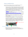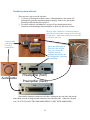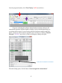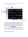
1
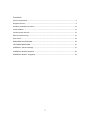
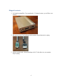
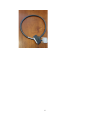
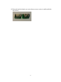
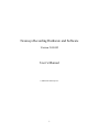
Neurosys Recording Hardware and Software Version 2.00.002 User’s Manual © 2008-2014 Neurosys LLC 1 Contents System requirements. ..................................................................................................................... 3 Shipped contents:............................................................................................................................ 4 Hardware assembly instructions: .................................................................................................. 10 Install software: ............................................................................................................................. 11 Conduct system self-test: .............................................................................................................. 12 Real-time spike sorting .................................................................................................................. 21 Spike Sorter ................................................................................................................................... 23 GROUNDING and SHIELDING: ....................................................................................................... 24 ELECTRODE FABRICATION ............................................................................................................. 25 APPENDIX 1, Software settings. .................................................................................................... 27 APPENDIX 2: Matlab integration ................................................................................................... 30 APPENDIX 3: Med-PC® integration................................................................................................. 32 2 System requirements. To use your system, you will need the following items: 1. 2. 3. 4. 5. Computer running Windows XP, 7, or 8. One free PCIe slot (a standard PCI slot will not work, it must be PCIe). At least 4GB of RAM. Speakers plugged into computer’s audio port, to listen to neural signals. If you have purchased a rat system, you will need a Med-Associates drug delivery arm and extra counterweight (part numbers PHM-115-SAI and FAB-PHM-110C) to hold the commutator. As of spring 2014, Med Associates charges $140 for both items together. The delivery arm is visible here: http://www.medassociates.com/products-page/self-administration/drug-delivery-arms-forrat/drug-delivery-arm-assembly-with-38-gimbal-ring/ It is best to purchase a second counterweight to balance the commutator - call Med Associates for the part number, as it is not listed on their website. 6. Materials for fabricating electrodes (connectors, insect pins, cutter, wire). Please see “Electrode Fabrication”, page Error! Bookmark not defined.. 3 Shipped contents: 1. 16-channel preamplifier. If you purchased a 32-channel system, you will have two of these. 2. (Rat systems only): Rat headstage with retention clips and protective spring 3. (Mouse systems only): Mouse headstage with 18” ultra-thin wire, no retention clips or spring. 4 4. DAQ board from National Instruments. Your board may say “M” series instead of “X” series, but they are functionally similar: 5. 24” cable to connect preamplifier and DAQ board. 5 6 6. Extension cable for preamplifier input, 60” long. This allows amplifier and computer to be some distance away from the recording chamber. 7. Commutator (rat system only) 7 8. Self-test board and stereo cable. The stereo cable is used to connect the self-test signal (delivered from back of preamplifier) to self-test board. The self-test board can plug into either the headstage (via the small white Omnetics connector) or to the preamplifier itself (via the large black connector) 9. 24VDC power adapter 8 10. Electrode interface boards (rat version shown, mouse version is smaller and lacks clip sockets) 9 Hardware assembly instructions: Note that the Neurosys hardware and software can be installed in either order. The software will run with simulated inputs if it does not find the A/D board. 1. Turn off your computer. Install the National Instruments digital acquisition board (“DAQ board”) into your computer’s motherboard. You must have one available PCIe slot. A regular (non-express) PCI slot will not work. If you have any other boards in your computer from National Instruments, I recommend removing them to simplify the installation. However, if you would prefer not to remove them, the program will prompt you by asking which card you want to use. 2. Install the drivers for the acquisition board. These are available by going to www.ni.com, and searching for “nidaq run-time engine”. As of March 7, 2014, the latest version of the nidaq driver is 9.8: http://www.ni.com/download/ni-daqmx-run-time-engine-9.8/4298/en/ If you have NIDAQ already installed, make sure it is at least version 9.6. Older versions may not work. 3. NIDAQ is huge. It will take a while to download and install – probably about an hour. You can (and should) go ahead and finish the rest of these steps while NIDAQ is installing. 4. Connect the preamplifier to the DAQ card with the 24” cable. The wide end of this cable plugs into the preamplifier (green arrow below) and the narrow end plugs into the back of the DAQ board. If you purchased a 32-channel system, there will be two preamplifiers, two cables, and two connectors on the DAQ board. One of the DAQ board connectors will be labeled “connector 0, ai0-15”, and the other will be labeled “connector 1, ai16-32”. Make note of which amplifier is plugged into which connector, as connectors 0 and 1 will appear in the software as recording chambers 1 and 2, respectively. AC adapter connects here Connect audio cable for self-test 24” cable connects here 5. Plug the 24V AC power adapter into the socket marked 24 VDC. 6. Rat systems only: install the commutator into your recording chamber. The commutator is designed to be held using a Med Associates drug delivery arm. It should simply snap into place. 10 Install software: Download the installer file from www.neurosysllc.com/Software.html and run it. It should install two programs: “NeuroPhys”, which is the main acquisition program, and “SpikeSorter”, which is an offline analysis program. Now launch the acquisition program by clicking this icon: You can also launch from Start menu ---NeurosysLLC ---Launch NeuroPhys. At first launch, NeuroPhys will ask you to register the product: Click “Register Product”. Then select “Import license from XML file”, and choose the license file you were sent. If you don’t have one, you can run a FREE version that is fully functional forever, but allows only 4 active channels. 11 Conduct system self-test: There are two ways to test the software: 1. If you are evaluating the software alone, without hardware, the system will automatically generate simulated signals to display. In this case, just launch NeuroPhys and skip directly to page 13. 2. To test the software with hardware, use the self-test board shown below. Connect it to the headstage and preamplifier as shown by the arrows below: The two white “Omnetics” connectors mate to each other. Each one has writing on one side and not the other – make sure writing faces same side or else pins won’t fit. Self-test board Connect audio cable here and to back of preamplifier Audio cable Headstage Ignore this black plug at first. But if the self-test fails, you can test the amplifier alone by plugging this directly into the preamplifier, bypassing the headstage. Preamplifier (front) Preamplifier (back) Note that the Omnetics connectors each have writing on only one side, and not the other. Make sure the writing on both connectors faces the same side – otherwise, the pins won’t fit. IF YOU HAVE TWO PREAMPLIFIERS, START WITH AMPLIFIER 1. 12 Once the program launches, click “Start Display” (RED arrow below): If you are evaluating the software without hardware, then the software will automatically generate simulated signals to display, and you should immediately see waveforms on the screen. If you are testing a physical hardware amplifier and DAQ board, you have to tell the system to generate a test waveform, by clicking “Channel Manager” (PURPLE arrow above), which will bring up a dialog with a grid: Click here to send test waveforms When this dialog opens, click the button “Start test signal for selected boxes”. 13 Your main window should now be filled with colorful waveforms, which update every 50 milliseconds. It will look like this, but more animated: Make sure “Show Spikes” is selected Use this option to listen to spikes on computer speaker A warning will appear down here if amplifier is not plugged into DAQ board, or is not turned on. If you do not see the signals above, make sure that the “Show Spikes” tab is selected, and that the preamplifier is connected to the DAQ board, and powered on. The software can automatically detect if the amplifier is plugged in, and if it is not, a warning will appear on the bottom status window. When warnings are present, the status window background will turn red, and the spike display window backgrounds will also acquire a reddish tint. If you still don’t see the above waveforms after double checking connections and power, please email me at [email protected], or call 843-882-7128. If you have two amplifiers, the test signal will only be sent to whichever box is currently “selected”, i.e. which box’s tab is displayed in the channel manager. To test the second chamber, stop the Test Signal (by pressing the same button you used to start it), then select the other chamber in the Channel Manager tab, and then restart the Test Signal. Channels are grouped by operant box: 14 If you bought a 16-channel system, the system will assume you have one operant chamber, and will assign all 16 channels to it. If you bought a 32-channel system, the system will assume you have 2 operant chambers, each with 16 channels of recording capacity. Data from these chambers (boxes) can be viewed and recorded independently. In this case, you’ll notice that there will be TWO tabs with spike windows. One will be labeled “Spikes, Box1”, and the other “Spikes, Box2”, and there will be 16 sub-windows in each tab. Likewise, the channel manager will also have one tab for each box, with each tab displaying 16 of the 32 total channels. If you have a 32-channel system, and want to change the defaults, e.g. assign all channels to a single box, then click the “Tools” menu, “Options”, “Basic ephys settings”, and change the setting “Active electrophysiology channels per chamber” from 16 to 32. Navigating the interface. After you start the self-test, the waveforms you see in each window will represent 50 milliseconds of data, i.e. 1/20th of a second. To take a closer look at waveforms for any channel, you can double-click on any panel, which toggles it to full-size, and hides the other 15 channels. You can also click “pause screen” (blue arrow below) to freeze the display. There is a row of buttons just below the main tool bar, that allows you to select “Session status”, “Show Spikes”, “Show Sort Clusters”, “Rasters”, “ISI” (interspike interval histograms), and “Field potentials”. These are fairly self-explanatory, except for “Sort Clusters”, which will be described later in this manual under “Sorting” (page Error! Bookmark not defined.). Switch to paneled view (best for widescreen monitors) Pause waveforms Show detected spikes Uncheck the “Mute Audio” box to listen to spikes on computer’s speaker Double-click any panel to toggle full screen Thin horizontal yellow line is threshold for initial spike detection 15 If you are interested in spike recordings, you will want to selectively view amplitudes that rise above background noise. The program can selectively display and save such waveforms. First, make sure that the “Show Spikes” tab is selected. Then click “Show thresholded” (PURPLE arrow above) to toggle “thresholded” mode, which only displays waveforms in which the voltage exceeds a set threshold. The threshold appears as a horizontal yellow line across each plot, which you can drag up and down with the mouse. If the threshold line seems to be missing, it is sometimes at the top or bottom edge of the window – simply grab it with the mouse to pull it back in. You can also set thresholds automatically by clicking and holding the “Auto threshold” button – this will set threshold to be 2 standard deviations below the mean voltage. You have to hold down this button for a second or two for this to take effect, and once you let go, the threshold will lock in place. In thresholded mode, you will see 800µs of each spike waveform, with 200µs shown before the threshold is hit, and 600µs shown after. These can be changed in the settings. Once a recording session starts, detected spikes will be saved to disk, but waveforms in between detected spikes will not be saved by default. You can also view field potentials, which are the input signals downsampled to one kilohertz. To see these, click on the “Field Potentials” tab. There is another button (green arrow above) that toggles between the default tabbed view, and a full-screen PANELED view. The latter mode allows you to see the cluster, ISI, and spike tabs simultaneously. PANELED mode is highly recommended, and works best with a widescreen monitor! Start a simple recording session: Once the self-test signals are visible on the screen, you can record them to a file. Click on the first tab labeled “Show session status”. Under the tab “Box status”, there should be a grid with one row for every recording chamber, and a green box in each row labeled “Start Ephys”, as shown below: 16 Click here to start recording from box 1 Remember to Start the Display first. Each channel is referenced to ground by default. However, if you have a dedicated reference wire, you can right-click on that channel, and select “reference all channels to this wire”. By default, ONLY DETECTED SPIKES are saved to disk. 17 Modifying what signals get recorded: If you click the right mouse button on any spike window, you will see this menu, which is used to modify how data is acquired and saved: Here is an explanation of each option: Enable spike recording: By default, detected spikes are saved for each channel. If you toggle this off, then detected spikes are not saved, and waveforms will display as grey instead of in color. You should disable spike recording for channels that do not appear to have any useful neural spikes. Store all samples: If selected (it is off by default) then all samples, not just detected spikes, are saved. Your file will become HUGE. Most of the time you do not want this. Reference all channels to this wire: Your preamplifier has hardware reference capability, i.e. the reference signal is subtracted before reaching the preamplifier. By default, all signals are referenced to ground, but you can select any channel to be a reference, i.e. its voltage will be subtracted from all other channels in this box. When you select this, all channels will have the same reference. If you want some channels to have one reference, and some to have another, you can do this too, but you must use the channel manager to do so. Reference all channels to ground: Self-explanatory. This is the default state when program is first launched. Make all thresholds like this: This refers to the threshold used to detect whether a spike has occurred or not. This option makes all channels in this box have the same threshold as the window you just clicked on. 18 Make all cursors like this: This refers to the vertical cursors used to calculate the voltages in the 2-D cluster plots. This option makes all channels have the same cursors as the window you just clicked. Exclude channel: This disables recording for this channel, similar to the effect of disabling “spike recording”. However, when a channel is excluded, its waveforms are no longer visible, not even in greyed out form. Also, excluding a channel will significantly reduce CPU load, because the computer will no longer have to calculate and display waveforms for this channel. For more precise control over recording settings, you can also use the “Channel Manager” to view and change all settings at a glance: 19 If you have more than one recording chamber configured, you will see one tab for each chamber, with the tabs being named “<Box1>”, “<Box2>”, etc. Unlike the menus above, the channel manager allows you to select a separate reference for each channel. In the above example, channels 1-7 are referenced to ground, while channels 9-12 are referenced to channel 8. The differential subtraction is performed prior to amplification, which allows for excellent common mode rejection. Any channel used as a reference will be highlighted in green. You can also exclude some channels from processing by checking the very last column “Exclude”. These channels will not be displayed, and no calculations will be performed on them, reducing CPU load. This should be done if some wires are not connected on a particular rat, or if a wire has gone bad and carries only noise. Excluding a channel will also prevent a user from accidentally recording from it, or using it as a reference for some other channel. Note that excluded channels still contribute to a system’s overall sample throughput. Hence, if you want to sample at a higher sampling rate than the default, you should reduce the number of active channels in the program “options”, rather than simply excluding them. Where is my data? By default, all recorded waveforms are saved to in the folder NeuroPhysData, under “My Documents”. Each session will generate two files: 1. A text (.TXT) file containing session log details – currently the session log shows the session duration, and any text sent by Med Associates programs running concurrently with the recording session. 2. A Plexon-format file (.PLX) containing spike timestamps and waveforms. You can change the folders by clicking “Tools”, “Options”. 20 Real-time spike sorting This system has the ability to “sort”, i.e. classify, spikes in real time. To demonstrate these capabilities, you can start a self-test session as described above. Then select “paneled” mode using the menu in the upper right of the main screen. When running the self-test, your screen will look something like this: Paneled mode Sort cluster display Horizontal line Voltage threshold Time cursor #1 Time cursor #2 In the example above, I have enlarged channel 1 by double clicking on it, so that it is the only spike channel visible. If you look closely, you’ll notice three cursors on this window, shown by yellow dashed lines: 1. A horizontal line that sets the voltage threshold at which a spike is detected. 2. A pair of vertical cursors that defines two time points. Each of these cursors can be adjusted by dragging it with the mouse. You’ll also see a panel in the upper right showing a bunch of dots that form “sort clusters”. The dots work as follows: 1. Each dot corresponds to one “detected spike”, i.e. one waveform that exceeds the specified voltage threshold. 21 2. The X and Y coordinates of each dot are the voltages at which each spike waveform intersects time cursor #1 and time cursor #2 respectively. This might seem confusing at first. To get some intuition on what is going on, note in the example above that the dots are mostly in the upper-left quadrant of the screen. That is because most of the waveforms intersect the first time cursor at a negative voltage (corresponding to an X value to the left of center), and the second cursor at a positive voltage (corresponding to a Y value above the center). There is another important property of the time cursors in the example above. I have placed time cursor #1 and #2 where the waveforms reach their approximate minimum and maximum voltages, respectively. This causes the dots corresponding to neural spikes to be as far as possible from background noise. Notice also how the dots segregate into multiple distinct clusters – these correspond to distinct neurons having distinct waveform shapes. You can click and drag the mouse to outline a polygon that encircles one of the clusters. This will cause all the waveforms corresponding to that cluster to display in a distinct color. You can place multiple polygons, and each will show up as a different color, with successive clusters receiving a designated letter “a”, “b”, “c”, etc. This designation is saved along with the spike timestamp and waveform during a recording session. The result should look something like the window below. You’ll see that I have outlined two clusters: When you complete a session, click on the red “Stop” button under the “Session Status” tab. This button is immediately next to the green button you clicked to start the session. You can now view your data file in the SpikeSorter program you have purchased. The icon for the SpikeSorter looks like this: 22 Spike Sorter The spike sorter is launched by clicking the following symbol: There is currently no manual for the SpikeSorter, but many of its features are similar to that of Plexon’s Offline Sorter, which can also be used to analyze the files produced by NeuroPhys. Just play around with it, and hopefully it is fairly self-explanatory. 23 GROUNDING and SHIELDING: When you implant electrodes into your rat, you will generally implant a ground screw into the cortex or cerebellum. This will somewhat shield the recordings from environmental noise, but it is generally not enough. Ideally you should shield the recording chamber from outside noise. There are many ways to do this. If you are using a metal recording chamber, the simplest way is to simply ground the walls and floor of the chamber. However, this will have the downside of introducing electromyographic (EMG) noise into the recordings whenever the rat touches the walls/floor. If you are only recording spiking activity, and not local field potentials, this might be acceptable because the EMG noise can largely be removed by placing an extra wire very close to the recording wires, and using it as a reference electrode. This will subtract away almost all EMG noise. Of course, it will also subtract away any local field potentials (LFP), so if you are interested in recording LFPs this is not recommended. If you are recording LFP’s, a preferred grounding method is to leave the chamber walls/floors floating, and ground the cabinet that the recording chamber is placed into. This can be done by placing metal foil or mesh on the walls of the enclosing cabinet. 24 ELECTRODE FABRICATION Electrode interface boards must be soldered onto Omnetics connectors (part number A79014-001). As of Feb 21, 2014, these connectors cost $35.26 each when purchased in quantities of 10 or more. For more info, see the following pages: http://www.omnetics.com/neuro/nano-strip/ http://www.omnetics.com/neuro/neuro_type.aspx?type=A79014001&category=nstrip Attaching the connector is not difficult, as the connector simply straddles the board in the obvious way. After an experiment is over, the connector and electrode board can be recovered by soaking the implant in acetone overnight. You should be able to recycle it about 4-5 times before it wears out. If you already use your own electrode designs, make sure it has one of the following Omnetics male connectors (with 18 signal pins and either 2 or 6 guide posts): 1. 2. 3. 4. 5. A79014 A79016 A79018 A79040 A79042 Omnetics also sells very similar looking connectors with 4 guide posts – you can NOT use them, as they have the signal pins in a 9x2 arrangement that will not fit the headstage. If you build your electrodes using the provided interface boards, you will also need stainless steel insect pins for binding wires into the holes. You can get these from Amazon.com, Indigo Instruments, or Bioquip. Make sure you get the STAINLESS pins. DO NOT ORDER THE BLACK PINS, as they black paint is NOT conductive. The exact pin size depends on the particular boards I sent you, but are usually #00, #0, or #1. I should have sent you some sample pins to get started. When you order more pins, they come in a package that looks like this: 25 You will need a cutter for snipping off the end of the insect pins. I recommend the Xuron 9180 Kevlar cutter: http://www.amazon.com/Xuron-XMS-9180-Finish-KevlarSerrated/dp/B00068P3TY/ref=sr_1_1?ie=UTF8&qid=1391901011&sr=81&keywords=kevlar+cutter . The cutter looks like this: You should cut the pins to a length of about 3-4mm. If you cut them too short, they will fall through the electrode board. If they are too long, that is actually workable, but the electrode will be unnecessarily large. Last but not least, you need electrode wire. I use A-M systems formvar-insulated nichrome wire (catalog # 761000). After the wires are pinned to the board, you will want to test that they are connected with a continuity tester. Once all wires are good, apply dental cement over the pins to lock them into place. 26 APPENDIX 1, Software settings. If you click on this wrench-like symbol , you will get a dialog with four pages of settings, which are detailed below: Page 1: “Data folders, behavior settings”. This page has the following settings: First Box ID. This sets the ID number of the first recording chamber. This is one by default. You can change it if you have multiple systems, and you want each physical box to have a unique ID number. For example, if you have two 32-channel systems, the first system’s recording chambers will have ID numbers 1 and 2 (the default) and you can set the second system to start numbering chambers at 3. Number of operant chambers. This sets the number of physical boxes in your system. By default this will be the same as the number of recording chambers, i.e. 1 for a 16channel system, and 2 for a 32-channel system. Behavior outputs per operant chamber. This is not used in the electrophysiology system, and is intended for controlling additional hardware such as levers, lights, pumps, etc. Timing resolution. This sets the resolution with which behavioral timestamps are recorded. In most cases, these timestamps will be received from external software, such as Matlab, Labview, Med-PC®, or other software. Ephys data folder. Folder to which standard ephys data (spikes and LFPs) will be saved. Wideband data folder. Folder to which wideband data will be saved. These files will be much larger than the spike and LFP files. 27 Page 2: Basic ephys settings ID of first electrophysiology box. By default this is the same as the first overall box ID. If you change the ID of the first overall box (e.g. from 1 to 3, in the example above), then this will change accordingly. This should be changed only if you have some operant chambers that are NOT configured for electrophysiology. Number of electrophysiology boxes. By default, this is simple the total system channels divided by 16. I.e. it will be 2 for a 32-channel system, and 1 for a 16-channel system. You should change this only if you are not using all available boxes, e.g. if you only want to use one box in a 32-channel system. This will reduce the number of displayed graphs, and also reduce the CPU load. Active electrophysiology channels per chamber. This sets the number of channels used per recording chamber. By reducing the number, you can achieve higher sampling rates, as the total system sampling rate is limited to 1MHz. Acquisition sample rate: This is a read-only field. It reports the achieved sampling rate. LFP acquisition rate. This is a read-only field that reports the sample rate for local field potentials (LFP). The next three radio buttons determine where the program will get its settings whenever it starts up. The choices are: 1. Load same settings that were in use when the program previously closed. 2. Load default settings. 3. Load settings from a particular file. Filter settings. All spike and LFP channels have optional software filters. These are: 1. Attenuate low frequencies. This option turns on a high-pass second-order butterworth filter that attenuates frequencies below the specified cutoff frequency. 2. Attenuate high frequencies. This turns on a low-pass second-order Butterworth filter that attenuates frequencies above the specified cutoff. 3. Attenuate low/high frequencies LFP. These options do the same thing, but for local field potentials. Subtract periodic noise. If checked, this setting activates an averaging algorithm that removes any noise with a periodicity of 60 Hz. Inverted inputs. If checked, this setting will invert the inputs, i.e. make negative voltages positive and vice versa. This should only be used if you have a preamplifier that has a negative gain value. Test waveform settings. This determines the type of waveform used for self-testing. 28 Page 3: Advanced electrophysiology settings. (This section has not been written yet) 29 APPENDIX 2: Matlab integration If you are controlling behavior from Matlab®, you will want to send behavioral event timestamps to NeuroPhys. To do this, use the following code, either from the Matlab prompt, or within a *.m file. If running 32-bit windows, first use the following: >> loadlibrary('c:\Windows\System32\NS_Library.dll', 'c:\Program Files\NeurosysLLC\NeuroPhys\NS_Library.h') If you are running under 64-bit windows use this line instead: >> loadlibrary('c:\Windows\SysWow64\NS_Library.dll', 'c:\Program Files (x86)\NeurosysLLC\NeuroPhys\NS_Library.h') If you are running this for the first time, you may be prompted to selected a compiler by typing “mex –setup”. The default, “lcc-win32” compiler will work fine. Now, within a Matlab program, the following functions are available: Calllib(‘NS_Library’, ‘NS_StartRecording’, boxNumber) This causes NeuroPhys to start recording spikes. “boxNumber” is an integer referring to the one-based operant chamber number. If you have only one chamber, this should always be one. Calllib(‘NS_Library’, ‘NS_SendEvent’, boxNumber, eventNumber, 0) This sends a timestamped event to NeuroPhys. When you later analyze the *.PLX file generated by NeuroPhys, this event will be recorded with a timestamp (in sample counts) at the moment this call was made. There will be a slight delay due to communication from Matlab to NeuroPhys, but this is typically only a few microseconds. boxNumber is the operant box number (one-based) as described above. eventNumber is a number between 0 and 511. The last argument (0) is not used. Calllib(‘NS_Library’, ‘NS_StopBox’, boxNumber) This causes NeuroPhys to stop recording spikes in the specified operant chamber. Calllib(‘NS_Library’, ‘NS_StartRecordingWideband’, boxNumber) This causes NeuroPhys to start recording wideband signals, i.e. it will record the raw voltages present at the A/D board inputs, without filtering away signals that are not 30 spikes. This will generate very large files, but you will have all possible information recorded. This is useful if you don’t know exactly how you will extract spike information, and wish to process the session off-line at a later time. 31 APPENDIX 3: Med-PC® integration Probably the best way to illustrate Med-PC® integration is with a sample MPC file. After installing NeuroPhys, this file will appear in “..\My Documents\NeuroPhysData”, along with a couple of sample data files: \ \ \ \ \ RecordingTest.MPC Simple test file to show communication between MedPC and NeuroPhys. ^LeftLever = 1 \ Left lever is output 1. If your chamber is wired differently, you should change this. s.s.1, s1, 0": ~sendeventname(BOX, 1, 'ProgramStart');~; ~sendeventname(BOX, 2, 'LeverPress');~; ---> S2 S2, #start: ~startRecording(BOX);~; ~sendtext(BOX, ‘Program starting’ + #13 + #10);~; ~sendevent(BOX, 1, 0);~; ---> S3 S3, #R^LeftLever: ~sendevent(BOX, 2, 0);~; ---> S4 S4, 5": ~stopBox(BOX);~; ---> StopAbortFlush Copy the above file from “My Documents\NeuroPhysData” into “C:\MED-PC IV\MPC”. Then compile it using TRANS®, and run it from Med-PC®. Make sure that NeuroPhys is already running before you run it. The command “StartRecording” will cause NeuroPhys to start recording spikes. This program will wait for a single press on the left lever, and then quite 5 seconds later. Note that all communication with NeuroPhys occurs via functions called from PASCAL, so all such functions begin and end with a tilde symbol. The command “sendevent” sends an event with the specified ID number (1 or 2 in the above example). The command “sendeventname” is optional, and is used to send a user32 friendly name to NeuroPhys, which will then write it into the PLX file header. When you later open your PLX file in the spike sorter, or in Neuroexplorer, these user-friendly names will appear, and will make your life a lot easier. Just before the Med-PC program ends, call “StopBox” to stop the recording session. If you forget to include this line, NeuroPhys will keep recording, and you will have to stop it manually (the red button on the box status tab). 33