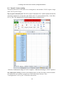
Download CurveAlign V1.3 Beta2 User`s Manual

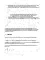
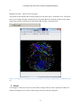
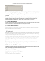
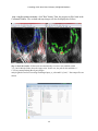
CurveAlign V1.3 Beta2 User’s Manual
1
Introduction ........................................................................................................................................... 2
2
QuickStart Instructions ......................................................................................................................... 3
3
Relationship with CT-FIRE .................................................................................................................. 3
4
Fiber processing modes ......................................................................................................................... 4
5
Boundary processing modes ................................................................................................................. 4
6
Input files .............................................................................................................................................. 5
7
Output data files .................................................................................................................................... 5
8
Output images ....................................................................................................................................... 6
9
8.1
Overlay image ............................................................................................................................... 6
8.2
Map Image .................................................................................................................................... 7
Stacks .................................................................................................................................................... 9
9.1
Stacks with Boundaries ............................................................................................................... 10
9.2
Stacks without Boundaries .......................................................................................................... 10
Batch mode ..................................................................................................................................... 10
10
10.1
Batch mode with CSV boundaries .............................................................................................. 10
10.2
Batch mode without boundaries .................................................................................................. 10
10.3
Batch mode with Tiff boundaries................................................................................................ 11
10.4
Batch mode with CT-FIRE input ................................................................................................ 11
11
Feature Ranking .............................................................................................................................. 11
12
Tutorials .......................................................................................................................................... 11
12.1
Tutorial 1: feature extraction with fiber extraction method “CT” and CSV boundary .............. 11
12.2
Tutorial 2: feature extraction with CT-FIRE method and Tiff boundary.................................... 14
12.3
Tutorial 3: feature ranking .......................................................................................................... 16
13
Status Label..................................................................................................................................... 18
14
Tips ................................................................................................................................................. 18
15
Acknowledgement .......................................................................................................................... 19
CurveAlign V3.0 Beta2 User’s Manual, LOCI@UW-Madison
1
Introduction
The purpose of CurveAlign is to compute features that describe collagen interactions with epithelial cells.
It was developed in order to search for stromal changes that are correlated with disease in images of
collagen and epithelial cells. We have recently used CurveAlign for the feature calculations performed in
a research paper by Bredfeldt, et. al. (Journal of Pathology Informatics, 2014, in press). Collagen images
may be obtained by a number of imaging approaches however we have focused here on Second
Harmonic Generation (SHG) images of collagen. Epithelial cell information is input into CurveAlign as
an 8-bit mask file, that must be pre-registered with the collagen image, where white pixels correspond to
epithelial cell regions and black pixels correspond to anything else in the image i.e. the background,
collagen fibers etc. These mask files can be generated by any appropriate means, such as manual ROI
annotation in FIJI or using segmentation tools in MATLAB or FIJI. The output features can then be used
to potentially classify images or fibers using machine learning techniques. An Support Vector Machine
(SVM) is incorporated into CurveAlign for ranking extracted features, and these features can also be used
or ranked through many open source machine learning tools such as Weka and R.
The primary change in CurveAlign Beta version 3.0 is feature extraction from CT-FIRE output.
Compared to the version 2.3, the major updates are : (1) output up to thirty four fiber features, including
angle, alignment, density, and etc. , these features are saved in both .cvs file and .mat file, which can then
be used to potentially classify images or fibers using machine learning techniques; (2) tiff boundary can
be loaded to investigate the interaction between fiber and cell boundary; (3) CT-FIRE fiber extraction
results can be read in; (4) a feature ranking using support vector machine (SVM) is included; and (5) keep
the most features of the older version (2.3), such as the statistics for the relative angles, heat map to show
the fiber(angle) alignment, and the fiber-boundary association, etc.
The GUI in CurveAlign is modular, so that the main user interface is in a separate window from the
outputs. This allows for the user to resize the output windows to their preferred size. The main user
interface window is shown below.
2
CurveAlign V3.0 Beta2 User’s Manual, LOCI@UW-Madison
In this manual, depending on the selected "Fiber analysis method" in the drop down box at the top of the
GUI, "fiber" may refer to curvelets that represent a fiber segment (CT), fiber segments generated by CTFIRE, the extracted fiber generated by CT-FIRE , or extracted fiber endpoints generated by CT-FIRE.
2
QuickStart Instructions
1) Select the fiber processing mode from among the following options- CT,CT Fire Segments, CT
FIRE endpoints and CT FIRE Fibers
2) Select the boundary processing mode from among the following options- No Boundary, CSV
Boundary , Draw Boundary and TIFF Boundary.
3) Click “Get Images” and browse to an image. Images may be single or stacks. If you would like to
process more than one image in a batch, just select more than one image in the dialog using the
technique appropriate for your operating system (i.e. in Windows, hold CTRL while selecting
multiple files).
4) If a manual boundary is required (not available in batch mode), hold down the Alt key and click
points along the desired path on the image window. Release the Alt key when finished.
5) Enter the keep threshold level if fiber extraction mode “CT” is selected, and select the desired
outputs using the checkboxes on the bottom of the main window.
6) Click the run button.
7) The output data and images will automatically be placed in a folder called CA_Out in the
directory with the original image(s).
8) If you have drawn a boundary, you will be prompted to give a file name and location for the
boundary points to be saved. These will be saved as a *.csv file. This file can be used again in the
future by selecting CSV boundary as the boundary processing mode. Store the boundary in the
same directory as the original image with the filename as "image.tif.csv" if the name of the
original image is" image.tif".
9) The current function being performed by CurveAlign is listed in the Status label at the bottom of
the main window.
3
Relationship with CT-FIRE
CT-FIRE is another software tool developed for processing images of fibers (Bredfeldt J., et al., Journal
of Biomedical Optics, 2014). CT-FIRE traces fibers and outputs a database of fiber objects. This output
database can be used as an input to CurveAlign (the subject of this manual). CurveAlign's main purpose is
to compare fibers with boundaries and fibers to each other to measure density and alignment. When CTFIRE inputs are used, the fibers are compared to region boundaries, either drawn manually, or created by
any segmentation tool.
CT-FIRE and CurveAlign may someday be combined, but the basic philosophy is that it is useful to
have them separate and easy enough to just connect them by reading the CT-FIRE outputs into
CurveAlign when needed.
3
CurveAlign V3.0 Beta2 User’s Manual, LOCI@UW-Madison
4
Fiber processing modes
There are four fiber processing modes. To avoid errors, ensure that the previously opened xls files of
results of an image are closed before any other operation is performed on the same image
1) Curvelet Transform: The curvelet transform is performed on the image(s) and each curvelet
corresponds to an observation in the feature list. Each curvelet has a unique angle and position. In
this case, fiber length and curvature are not available, since curvelets are independent from one
another.
2) CT-FIRE Segments: The output from CT-FIRE is used as the input, providing information about
the fibers in the image. Each fiber segment in the CT-FIRE output file corresponds to an
observation in the feature set. Each segment has a unique angle and position. In this case, each
segment is given a fiber length and curvature value that corresponds to the length and curvature
of the entire fiber this segment belongs to. For this option, the .mat file generated by CT-FIRE
must be saved in the same folder as the original .tif image, and when prompted the.tif image
should be selected.
3) CT-FIRE Fibers: The output from CT-FIRE is used as the input, providing information about the
fibers in the image. Each fiber center point in the CT-FIRE output file corresponds to an
observation in the feature set. Each center point has a unique angle corresponding to the average
angle of the fiber. The position is the midpoint between the fiber end points. In this case, each
center point is given a fiber length and curvature value that corresponds to the length and
curvature of the entire fiber this center point belongs to. For this option the .mat file generated by
CT FIRE must be in the same folder as the original .tif image, and when prompted the.tif image
should be selected.
4) CT-FIRE Fiber Endpoints: The output from CT-FIRE is used as the input, providing information
about the fibers in the image. Each fiber endpoint in the CT-FIRE output file corresponds to an
observation in the feature set. Each endpoint has a unique angle and position. The angle
corresponds to the angle of the entire fiber. In this case, each endpoint is given a fiber length and
curvature value that corresponds to the length and curvature of the entire fiber this segment
belongs to.
When CT-FIRE outputs are used as inputs to CurveAlign, the CT-FIRE output files must be named
according to a strict naming convention. For example, if the image is named the following:
1B-a1.tif
Then the CT-FIRE output file must be named the following:ctFIREout_1B-a1.mat
At the time of writing this manual, the above naming convention has been adopted by the CT-FIRE tool
as well, so the outputs from CT-FIRE may be directly used as inputs to CurveAlign.
5
Boundary processing modes
There are four boundary processing modes.
1) No boundaries: Fibers will be compared to each other, but not to a boundary. For example,
features about fiber alignment will still be computed and output in the feature list.
4
CurveAlign V3.0 Beta2 User’s Manual, LOCI@UW-Madison
2) Manual boundaries: The user is required to manually draw boundaries with the Alt-key + mouse
clicking technique. This option is not allowed if multiple input images are selected to be
processed in a batch. If this option is selected and multiple files are to be processed, then the "No
Boundaries" option is automatically selected. All boundary points must be selected in a
succession, to select a new boundary click anywhere on the image and then select a new
boundary.
3) CSV boundaries: Previously stored boundary files can be used that contain the x-y positions of
points along the boundary.
a. CSV files must adhere to the following naming convention. If the image is named:
TACS-3a.jpg, then the CSV file must be named: boundary for TACS-3a.jpg.csv.
b. The boundary file must be in the same directory as the original image.
4) Tiff boundaries: Mask files are used to indicate where region boundaries are located. The mask
files should be 8-bit files where the inside of ROIs are given a value of 255 and outside a value of
0. This allows for features identifying whether a fiber is inside an ROI or not. These files must be
in pixel for pixel registry with the image files and therefore have the same dimensions as the
image files. Tiff boundary files must adhere to the following naming convention. If the image is
named: 1B-a5.tif, then the tiff boundary file must be named: mask for 1B-a5.tif.tif . The boundary
file must be in the same folder as the original image
When boundaries are used as part of the analysis, CurveAlign computes up to 2 relative angles per
observation. The first is the nearest point angle and the second is the intersection point angle. The nearest
point angle is the relative angle between the observation point and the tangent angle of the region
boundary at the point nearest to the observation point. The intersection point angle is the relative angle
between the observation point and the intersection point of the fiber, interpolated out a user defined
distance, and a boundary.
6
Input files
CurveAlign requires up to three types of input files.
Image files: These files contain images of fibers. These can be produced by any method available,
however we have particularly focused on SHG images of collagen fibers.
CT-FIRE files: The output of CT-FIRE having been run on the above mentioned "Image files."
Boundary files: The boundary files can be CSV files or Tiff files. See the section about Boundary Modes
above to learn about naming conventions for these file types.
.mat files must be present in the same directory as the original image while using the results of the CT
FIRE results.
7
Output data files
There are several files that are generated by the CurveAlign software for each image processed. These
files and their descriptions are listed in the table below:
5
CurveAlign V3.0 Beta2 User’s Manual, LOCI@UW-Madison
Filename
*_hist.csv
*_values.csv
*_stats.csv
*_fibFeatNames.csv
*_fibFeatures.csv
*_fibFeatures.mat
compFeat.mat
featRank.txt
8
Description
List of bin values and numbers of observations in each bin. Bin
values correspond to relative angle in if boundaries are used, and
absolute angle if no boundary is used.
relative angles as in version 2.3(using the nearest distance the
defined the region of interest)
Statistics of the relative angles as in version 2.3
Names of the 34 features
34 features in 34 columns in the order in *_fibFeatNames.csv
Features that can be used for the feature ranking here
Feature ranking output: feature array and meta array
Feature ranking output, including feature importance and
normalized feature difference between two classes
Output images
A few output images are saved in .tiff format in the selected output directory. These images are explained
below.
8.1 Overlay image
This image shows the position of each fiber detected within the particular distance from the user defined
boundary. The fibers outside the specified distance are also plotted for
Figure 1. Overlay image showing the fibers that are within or outside the specified distance. The
green lines show the fibers inside the specified distance. The red lines show the fibers outside the
specified distance. The boundary is the line connecting the yellow mark “*”. Blue lines are the lines
connecting the centers of the fibers with the nearest points on the user defined boundary.
6
CurveAlign V3.0 Beta2 User’s Manual, LOCI@UW-Madison
8.2 Map Image
The map image is intended to help the user identify the spatial distribution of fiber angles within the
image.
The raw map (_rawmap.tiff) file codes the angle of the fiber into a grey scale value. The pixel in the
image where the center of the fiber is located is given a value between 0 and 255 that corresponds to 0 to
90 degrees when a boundary is selected and 0 to 180 degrees when a boundary is not selected. This file
may be further processed in matlab or imagej according to the users preferences.
The processed map file (_procmap.tiff) is a processed version of the raw map file overlaid on the original
image. The output is intended to show regions of aligned structures that are perpendicular to the
boundary, in the case of a boundary selection, or regions of generally aligned structures, in the case where
no boundary is selected.
How processed map files are created:
When a boundary is selected, the raw map file translates 0 to 90 degrees into 0 to 255 in gray scale. The
center location of each curvelet is given a gray level corresponding to its angle with respect to the
boundary. Then a square max filter is applied with a size of 12 pixels on a side, followed by a Gaussian
disc filter with a sigma of 4 pixels. The color scale is then set to 0-10 degrees = black, 10-45 degrees =
green, 45-60 degrees = yellow, and 60-90 degrees = red. The map image is overlaid on the original image
with transparency set to 0.5 as shown in Error! Reference source not found..
Figure 3. Map image of the overlay image showing the fibers that are within the specified
distance.
7
CurveAlign V3.0 Beta2 User’s Manual, LOCI@UW-Madison
When a boundary is not selected, the raw map file translates 0 to 180 degrees into 0 to 255 in gray scale.
In this case, red indicates areas of highly aligned structures, while black and green indicate areas of more
randomly aligned structures. The map image is overlaid on the original image with transparency set to 0.5
as shown in Error! Reference source not found..
Figure 2. Overlay and map images when no boundary is selected.
Boundary Analysis
The user is able to analyze the fibers that fall only within a certain distance from a boundary. To enter this
distance, first a boundary must be drawn or opened from file. Then the distance in pixels should be
entered into the edit box.
Boundaries are created by alt-clicking on the original image that is opened in the CurveAlign GUI. When
alt is released, the boundary is ended and no additional points may be added to the boundary. If the
boundary mode “CSV Boundary” or “Tiff Boundary ” is selected, previously saved boundary file can be
automatically checked and loaded in if it exists. The boundary file should be saved in the same directory
as the selected image and should be named like the following:
Image file name = TACS-3a.jpg
Boundary file name = boundary for TACS-3a.jpg.csv
8
CurveAlign V3.0 Beta2 User’s Manual, LOCI@UW-Madison
or
Boundary file name = mask for TACS-3a.jpg.tif
The position on the boundary that is being compared to each fiber may be visualized as well. This allows
the user to see where the angle comparisons are being made. Blue lines are drawn on the overlay output
image from each fiber to the point on the boundary that the fiber is associated with.
Figure 3. An example of an overlay images where the associations between fibers and the boundary are indicated by blue
lines.
9
Stacks
CurveAlignV3.0 allows for the user to select stacks of images. When a stack is opened, the slider bar is
enabled, allowing the user to choose which image in the stack should be displayed.
9
CurveAlign V3.0 Beta2 User’s Manual, LOCI@UW-Madison
When a stack is being analyzed, then the output files that are images will also be in stack format. To open
these stacks in ImageJ, the LOCI bioformats importer must be used. For some reason, these tiff stacks
cannot be drag and dropped into ImageJ, this will be investigated further in the next release of
CurveAlign.
The other output files, for example the histogram file and the curvelet angle spreadsheet, are produced
such that each image in the stack creates a new output file. For example a stack with 4 images will
generate 4 histogram files named stack_1_hist.csv, stack_2_hist.csv, stack_3_hist.csv, etc.
9.1 Stacks with Boundaries
If a stack is being processed, then only a single boundary can be used for the entire stack. Future versions
of this tool will allow for a different boundary in each image plane in a stack.
9.2 Stacks without Boundaries
When no boundary file is selected, then each image in the stack is analyzed as described in the section
above about image analysis without a boundary.
10 Batch mode
Batch mode is used to process multiple images and potentially associated boundaries. To use batch mode,
click the Get Images button and select more than one image in the file selection dialog box. Each image
will be processed according to the modes currently selected.
CurveAlign will first search for boundary files in the chosen directory. If there are boundary files, then it
will process all images that are found to be associated with the located boundary files. Images may be a
mixture of both individual images and stacks. If the image is a stack, then the entire stack will be
processed.
The batch mode output files will be stored in a directory named CA_Out and will include all of the
outputs available from the CurveAlign software.
10.1 Batch mode with CSV boundaries
If boundaries are drawn with the CurveAlign program, they should be saved in the same directory as the
images. The boundary files should be named like the following:
Image file name = TACS-3a.jpg
Boundary file name = boundary for TACS-3a.jpg.csv
10.2 Batch mode without boundaries
10
CurveAlign V3.0 Beta2 User’s Manual, LOCI@UW-Madison
To process a directory of images without boundaries, then just place the images in a directory by
themselves (without any boundary files), then run CurveAlign with select all of the images in that
directory. In this case, the distance from the boundary and boundary association edit boxes will be
ignored.
10.3 Batch mode with Tiff boundaries
In batch mode, boundaries may also be imported as tiff files. Tiff boundary files must be 8bit binary mask
images where the inside of a region has a value of 255 and everything else must be 0. Boundary tiff files
must have the same number of pixels (length and width) as the original image and may be produced by
hand or by segmentation in ImageJ/FIJI. Tiff boundary files should be named according to the following
convention:
Image file name = 1B-a5.tif
Boundary file name = mask for 1B-a5.tif.tif
10.4 Batch mode with CT-FIRE input
To compare the results of the CT-FIRE software to boundaries (either TIFF or csv), then choose one of
the CT-FIRE fiber processing modes on the main GUI. The following naming convention should be
strictly used:
Image file name = 1B-a1.tif
CT-FIRE results file = ctFIREout_1B-a1.mat
11 Feature Ranking
Based on the importance for differentiating two-class classification problem (Negative and Positive)
using SVM, SVM feature weight is used to rank the features. The average feature value difference
between two classes is also included. An annotation file including the label for each image is
needed to be prepared before running the feature ranking. This file is named as "annotation.xlsx"
with two columns, where the first column includes the label for each image( e.g.: 1 for positive,
0: negative ), the second column includes the full original image name.
12 Tutorials
To reproduce the tutorials, users need to first download the test images and boundary files at LOCI
website.
12.1 Tutorial 1: feature extraction with fiber extraction method “CT” and CSV boundary
Step 1 choose the methods of fiber extraction and boundary, open an image: As shown in the
Figure below, Select the "CT" as the Fiber analysis method, "CSV Boundary" as the Boundary
method and then click the "Import image/data" button. A file selection window opens allowing
the user to choose the image. In this tutorial, "TACS-3a.jpg" is selected.
11
CurveAlign V3.0 Beta2 User’s Manual, LOCI@UW-Madison
Step 2 select run parameters and set output options: After clicking "Get Images", the image is
displayed and new controls are enabled on the control panel as shown below, and information
shown in the command window "Found boundary for TACS-3a.jpg.csv" indicates the CSV
boundary file was found. The fraction of curvelets coefficients is set to "0.005", the region of
interest is set to the area within the 150 pixels distance from the boundary. All the output
options are checked.
12
CurveAlign V3.0 Beta2 User’s Manual, LOCI@UW-Madison
Step 3 run fiber feature extraction: click "Run" button. Then, the progress will be listed in the
Command Window. The overlaid and map images will also be displayed as follows
Step 4 check the results: All the results are automatically saved to a new subfolder called
"CA_Out"within the folder where the image exists. In this case, the path for this subfolder is "
C:\Users\youmap\Desktop\Box Sync\collagen
analysis\github\curvelets\CurveAlignTestImages\input_ct_csvbound\CA_Out\)". Nine output files are
shown:
13
CurveAlign V3.0 Beta2 User’s Manual, LOCI@UW-Madison
Step 5 reset the GUI: Click "Reset" to start over .
12.2 Tutorial 2: feature extraction with CT-FIRE method and Tiff boundary
Step 1 choose the methods of fiber extraction and boundary, open an image: As shown in the
Figure below, Select the "CT-FIRE Fibers" as the Fiber analysis method, "Tiff Boundary" as the
Boundary method and then click the "Import image/data" button, a file selection window opens
allowing the user to choose the image. In this tutorial, " 1B-a1b.tif" is selected.
Step 2 select run parameters and set output options: After clicking "Get Images", the image is
displayed and new controls are enabled on the control panel as shown below, and the information
shown in the command window " Found ctFIREout_1B-a1b.mat, Found mask for 1B-a1b.tif.tif"
indicates the CT-FIRE output file and Tiff boundary file were found. The region of interest is set
to the area within the 300 pixels from the boundaries. All the output options are checked.
14
CurveAlign V3.0 Beta2 User’s Manual, LOCI@UW-Madison
Step 3 run fiber feature extraction: click "Run" button. Then, the progress will be listed in the
Command Window. The overlaid and map images will also be displayed as follows
Step 4 check the results: All the results are automatically saved to a new subfolder called
"CA_Out"within the folder where the image exists. In this case, the path for this subfolder is
C:\Users\youmap\Desktop\Box Sync\collagen
analysis\github\curvelets\CurveAlignTestImages\input_fire_tiffbound\CA_Out\)". Eight output files are
shown. Compared to the output of the tutorial 1, the CT-reconstructed image is not available here.
Step 5 reset the GUI: Click "Reset" to start over .
15
CurveAlign V3.0 Beta2 User’s Manual, LOCI@UW-Madison
12.3 Tutorial 3: feature ranking
This tutorial shows how to rank features for a training data set that includes 8 TACS-3 negative images
and 8 TACS-3 positive images.
Step 1 prepare annotation file: The file is named "annotation.xlsx" which contains the label for
each image and must be saved in the same folder as the CA extracted feature files, i.e the foder
of /CA_Out/. The annotation file for this training images is shown below,
wherein, 0 indicates the image is TACS-3 negative, 1 indicates the image is TACS-3 positive
Step 2 Run feature ranking: click the Feature Ranking button, all other fiber feature extraction buttons
are "enabled off" and a window is popped up to "Select fiber feature directory". Here,
"\TrainingSets20131113\CA_Out\" is selected as shown below
16
CurveAlign V3.0 Beta2 User’s Manual, LOCI@UW-Madison
After clicking OK, two windows pop up as shown below. One is the CA Features List showing the index
and description of each of the 34 features , the other is a input dialog window which shows the applicable
features and can be used to enter the number of the features to be ranked. In this tutorial, enter " 6, 8:9,
14:18, 23:32 " as shown below , i.e features [6 8 9 14 15 16 17 18 23 24 25 26 27
28 29 30 31 32]. User can input arbitrary number of features to be ranked.
17
CurveAlign V3.0 Beta2 User’s Manual, LOCI@UW-Madison
After clicking "OK" button on the feature selection window, feature ranking starts and the two output
windows are displayed as below, including both the feature classification importance and feature
normalized difference between Negative and Positive classes.
The ranking results are saved in a txt file named "featRank.txt", which is saved in the same folder as the
.mat feature files.
13 Status Label
To allow the user to keep track of what is happening in the program, there is a status label on the bottom
of the main window. This label gives hints about what the user should do next or shows the current task
that the program is working on.
14 Tips
1) Output data and images are saved under a subfolder named \CA_Out\ within the folder where the
original image exists, and under filenames indicating the source of the data and the type of output.
2) To read in the output files from CT-FIRE, CT-FIRE output .mat files should be saved in the same
folder as the original images.
3) To read in the boundary files (in .csv or .tif format), the boundary files should be saved in the
same folder as the original images and should follow the strict naming convention, e.g., if image
18
CurveAlign V3.0 Beta2 User’s Manual, LOCI@UW-Madison
is named: "1B-a5.tif", CSV boundary is named "Boundary for 1B-a5.tif.csv", and tiff boundary is
named " mask for 1B-a5.tif.tif "
4) Tiff boundary files must be 8bit binary mask images where the inside of a region has a value of
255 and everything else must be 0. Boundary tiff files must have the same number of pixels
(length and width) as the original image and may be produced by hand or by segmentation in
ImageJ/FIJI.
5) Tiff boundary is recommended for more accurately extracting the features of collagen-cell
interaction.
6) -To run feature ranking, an annotation .xlsx file should be prepared and saved in the same folder
as the .mat feature files. This file is named as "annotation.xlsx" with two columns, where the first
column includes the label for each image( e.g.: 1 for positive, 0: negative ), the second column
includes the full original image name.
15 Acknowledgement
Guneet Singh Mehta has contributed to this manual.
19