Download Special Report No. 16 GREAT-ER User Manual

1
GREAT-ER User Manual
Special Report No. 16
GREAT-ER User Manual
March 1999
European Centre for Ecotoxicology
and Toxicology of Chemicals
Avenue E Nieuwenhuyse 4 (Bte 6)
B - 1160 Brussels, Belgium
2
ECETOC Special Report No. 16
CONTENTS
INTRODUCTION........................................................................................................................................... 1
1. INSTALLATION ....................................................................................................................................... 3
1.1 REQUIREMENTS........................................................................................................................... 3
1.2 SET-UP........................................................................................................................................... 3
1.3 GREAT-ER AND ArcView .............................................................................................................. 5
2. TUTORIAL ............................................................................................................................................... 6
2.1 BASIC CONCEPTS ........................................................................................................................ 7
2.1.1 Scenario Concept................................................................................................................. 7
2.1.2 Substance Database............................................................................................................ 8
2.1.3 Expert Mode vs. Easy-To-Use Mode ................................................................................... 8
2.1.4 Model System ...................................................................................................................... 9
2.1.5 Parameter Handling ............................................................................................................. 9
2.2 STARTING GREAT-ER................................................................................................................ 10
2.3 SETTING UP A SCENARIO ......................................................................................................... 11
2.3.1 Creating a New Scenario ................................................................................................... 11
2.3.2 Needed Inputs.................................................................................................................... 15
2.3.3 Editing Substance Data...................................................................................................... 16
2.3.4 Pick Substance and Change Database ............................................................................. 18
2.3.5 Editing Catchment Data ..................................................................................................... 19
2.4 RUNNING A SIMULATION........................................................................................................... 21
2.4.1 Save a Scenario................................................................................................................. 26
2.5 ANALYSING MODEL RESULTS.................................................................................................. 28
2.5.1 PEC Calculations ............................................................................................................... 28
2.6 ADDITIONAL DISPLAY OPTIONS............................................................................................... 32
2.7 DATA EXCHANGE ....................................................................................................................... 34
2.8 LIMITATIONS ............................................................................................................................... 35
2.8.1 ArcView .............................................................................................................................. 35
2.8.2 User Interface .................................................................................................................... 35
2.8.3 Model System .................................................................................................................... 37
2.9 ADDING A NEW CATCHMENT ................................................................................................... 37
3. MENU STRUCTURE.............................................................................................................................. 39
3.1 GREAT-ER ................................................................................................................................... 39
3.1.1 New Scenario..................................................................................................................... 39
3.1.2 Open Scenario ................................................................................................................... 39
3.1.3 Edit Scenario...................................................................................................................... 40
GREAT-ER User Manual
3
3.1.4 Close Scenario.................................................................................................................. 40
3.1.5 Save Scenario................................................................................................................... 40
3.1.6 Save Scenario As.............................................................................................................. 40
3.1.7 Delete Scenario................................................................................................................. 41
3.1.8 Export / Import .................................................................................................................. 41
3.1.9 Report ............................................................................................................................... 41
3.1.10 Expert Mode / Easy-to-use Mode...................................................................................... 42
3.1.11 Exit .................................................................................................................................... 42
3.1.12 n a scenario title ............................................................................................................... 42
3.2 SUBSTANCE................................................................................................................................ 42
3.2.1 New Substance ................................................................................................................. 42
3.2.2 Open Substance ............................................................................................................... 44
3.2.3 Pick Substance ................................................................................................................. 44
3.2.4 Edit Substance .................................................................................................................. 44
3.2.5 Close Substance ............................................................................................................... 44
3.2.6 Save Substance ................................................................................................................ 45
3.2.7 Delete Substance.............................................................................................................. 45
3.2.8 Change Database ............................................................................................................. 45
3.3 CATCHMENT ............................................................................................................................... 45
3.3.1 Select Catchment.............................................................................................................. 45
3.3.2 Select Subcatchment ........................................................................................................ 45
3.3.3 Unselect Subcatchment .................................................................................................... 46
3.3.4 Edit Market Data ............................................................................................................... 46
3.3.5 Edit Discharge-site Data ................................................................................................... 46
3.4 MODEL ......................................................................................................................................... 47
3.4.1 Select Model ..................................................................................................................... 47
3.4.2 Edit Model Parameters...................................................................................................... 47
3.4.3 Background Concentration ............................................................................................... 48
3.4.4 Start Simulation................................................................................................................. 48
3.4.5 Stop Simulation ................................................................................................................. 48
3.5 ANALYSIS .................................................................................................................................... 49
3.5.1 Calculate River Csim X ..................................................................................................... 49
3.5.2 Csim Classes River........................................................................................................... 49
3.5.3 Combine Csim / Flow........................................................................................................ 49
3.5.4 PECinitial........................................................................................................................... 50
3.5.5 PECcatchment .................................................................................................................. 50
3.5.6 Discharge Influent Csim / Discharge Effluent Csim .......................................................... 51
3.5.7 Concentration Profile......................................................................................................... 51
3.5.8 Export Profile..................................................................................................................... 51
4
ECETOC Special Report No. 16
3.6 DISPLAY....................................................................................................................................... 51
3.6.1 Add Background Data ........................................................................................................ 52
3.6.2 Remove Background Data................................................................................................. 52
3.6.3 Full Catchment Extent........................................................................................................ 52
3.6.4 Zoom In .............................................................................................................................. 52
3.6.5 Zoom Out ........................................................................................................................... 52
3.6.6 Show River Flows .............................................................................................................. 53
3.6.7 Select Rivernet by Flow...................................................................................................... 53
3.6.8 Identify................................................................................................................................ 53
3.6.9 Show Site Pictures ............................................................................................................. 53
3.6.10 Remove Themes............................................................................................................... 54
3.7 GREAT-HELP............................................................................................................................... 54
3.7.1 Contents............................................................................................................................. 54
3.7.2 About GREAT-ER .............................................................................................................. 54
3.7.3 About Model ....................................................................................................................... 54
4. GREAT-ER MESSAGES........................................................................................................................ 55
4.1 CONVENTIONS ........................................................................................................................... 55
4.2 HINTS ........................................................................................................................................... 55
4.3 WARNINGS.................................................................................................................................. 56
4.4 ERRORS ...................................................................................................................................... 59
APPENDIX A. CHEMICAL FATE SIMULATOR AND MODELS............................................................... 66
A.1 CHEMICAL FATE SIMULATOR................................................................................................... 66
A.2 CHEMICAL FATE MODELS ........................................................................................................ 67
APPENDIX B. HYDROLOGICAL MODELLING WITHIN GREAT-ER ...................................................... 70
B.1 INTRODUCTION.......................................................................................................................... 70
B.2 THE UK MODELS AND THE RIVER NETWORK BASED MODEL FRAMEWORK .................. 71
B.3 THE HYDROLOGY OF THE LAMBRO PILOT STUDY ............................................................... 82
BIBLIOGRAPHY ......................................................................................................................................... 87
MEMBERS OF THE TASK FORCE ........................................................................................................... 89
MEMBERS OF THE SCIENTIFIC COMMITTEE........................................................................................ 91
1
GREAT-ER User Manual
INTRODUCTION
Risk represents the likelihood that the hazard will be realised - i.e. that due to the exposure an adverse
effect may occur.
Risk assessment is defined as the process that evaluates the likelihood that
adverse ecological or human health effects may occur, are occurring, or have occurred as a result of
exposure to one or more physical, chemical, or biological agents.
Fundamental to the risk assessment definition is the recognition that risk requires two elements: (1) a
chemical or material’s inherent ability to cause adverse effects and (2) the exposure or interaction of
the chemical or material with an ecological component or with a human population at sufficient
intensity and duration to elicit the adverse effect(s). The risk assessment process is a step-wise
process in which assessment of potential adverse effects and exposure is integrated and compared
with increasing realism.
The ratio of the Predicted Environmental Concentration (PEC) to the
Predicted No Effect Concentration (PNEC) is used as a measure of this risk.
The assessment of risk can require an in-depth assessment of the intrinsic physico-chemical
properties, biodegradability, bioaccumulation potential and hazard or potential effects of the chemical.
In addition, a thorough assessment of the release pathway, environmental fate and distribution of the
chemical is required based on exposure measurements and/or mathematical models. In environmental
exposure assessment the concentration of a substance in the different environmental compartments is
estimated based on physico-chemical properties, the production and emission processes, the use and
disposal patterns and the properties of the environmental compartments.
Since the introduction of risk assessment legislation in the EU, separate guidance documents have
been prepared for the evaluation of risk for both New and Existing Chemicals (1993 and 1994,
respectively). Because the Risk Assessment Directive of New Substances and Risk Assessment
Regulation of Existing Substances were supported by a number of different technical guidance
packages which resulted in different risk assessment conclusions, and possibly could lead to different
risk management strategies, the Commission agreed to develop a uniform guidance package. This
package (EEC, 1996) was released together with the supporting risk assessment computer model
EUSES (European Uniform System for Evaluating Substances, 1996). The EUSES modelling
approach estimates PECs for fictive environments via a generic multimedia ‘unit world’ approach and
does not account for spatial and temporal variability in landscape characteristics, river flows and/or
chemical emissions. Hence, the results are merely applicable on a generic screening level since these
models do not offer a realistic prediction of actual steady-state background concentrations. In addition,
the default EU generic regional environment (EEC, 1996) assumes treatment of only 70% of the waste
water mass loading, leaving 30% of mass loading to this generic region untreated.
2
ECETOC Special Report No. 16
The objective of the GREAT-ER project is to develop and validate a powerful and accurate chemical
exposure prediction tool for use within the EU environmental risk assessment schemes. This new
database, model and software system is developed to calculate the distribution of PECs, both in space
and time, of down the drain chemicals in European surface waters on a river and catchment area
level.
The GREAT-ER software system uses a Geographic Information System (GIS) for data storage and
visualization, combined with simple mathematical models for the prediction of chemical fate.
Hydrological databases and models have been used to determine river flows in the pilot study areas.
GREAT-ER provides an accurate prediction of aquatic chemical exposure and allows the calculation
of a realistic distribution of environmental concentrations of down-the-drain chemicals for use within
the EU environmental risk assessment schemes. The aim of GREAT-ER is to enable the prediction of
the concentrations of chemicals at any specific location in EU rivers and river basins from site-specific
discharges, river and effluent flow data. The methodology delivered is applicable for the entire EU, but
the prototype runs in the first instance for the Aire, Calder, Went, Don (UK) and Lambro (I) regions,
and for parts of Belgium and Germany.
The refined exposure assessment tool should greatly enhance the accuracy of current local and
regional exposure estimation methods, and ultimately allow assessments on a pan-European scale.
This special report will allow you to install GREAT-ER and help you with key questions on how to run
GREAT-ER.
GREAT-ER User Manual
3
1. INSTALLATION
1.1 REQUIREMENTS
GREAT-ER is a collection of models and scripts set on top of the geographic information system (GIS)
ArcView, a product developed and marketed by the Environmental Systems Research Institute (ESRI).
The development was based on the software package ArcView 3.0 with the patch for version 3.0a.
GREAT-ER is also compatible with the new version ArcView 3.1.
The operating system GREAT-ER is designed for WINDOWS NT 4.0. Please note that GREAT-ER will
not work properly under W INDOWS 95 although ArcView 3.0 and 3.1 do. Compatibility with W INDOWS
98 was not tested.
The GREAT-ER system contains a set of scripts for ArcView, models and other programs for data
analysis. It also comes with a set of data and additional information for selected pilot regions.
The installation requires a minimum free hard disk space of approximately 50 MB.
1.2 SET-UP
GREAT-ER comes with its own set-up program, specifically designed for the installation of the
complete modelling system. It can be found in the root directory of the GREAT-ER CD-ROM. It is
recommended to exit all other running applications while installing GREAT-ER on your computer.
Installation steps (some terms are language dependent and may be different on your W INDOWS NT 4.0
version):
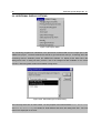
1. Insert the GREAT-ER CD-ROM into your CD-ROM drive. Run the setup program by selecting
"Execute" from the W INDOWS NT 4.0 "Start Menu". Type e.g. \setup.exe and click the "OK"
button. Please note that D may have to be replaced by the letter of your CD-ROM drive.
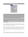
2. The first dialog appears, showing you the licence text of GREAT-ER. Please ensure you have
carefully read and understood all the terms of the licence agreement. If you agree to the licence
agreement, proceed with the installation by clicking the "Accept" button. If not, select "Cancel". The
installation will then be aborted and GREAT-ER will not be installed on your system. At any time
during the installation you can return to a previous dialog to modify settings by clicking the "Back"
button.
4
ECETOC Special Report No. 16
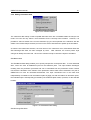
3. Select the type of installation: either full installation or CD-based installation. It is recommended to
proceed with the full installation. The CD-based installation should only be chosen for evaluation
purposes. The required disk space is reduced to the amount of data resulting from simulation
runs; all scripts, programs and additional data are loaded for a GREAT-ER application from the
CD-ROM. This means the CD-ROM needs to be inserted in your CD-ROM drive while working with
GREAT-ER. On the other hand, it is not possible to add new substances to the systems data base
or to include further catchments or additional geo-referenced data.
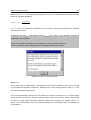
4. If you have selected the full installation, the following dialog will enable you to specify the directory
in which to install GREAT-ER. A directory can be specified by typing in the path directly or by
browsing through the directory tree. If you type in a non-existing directory, the setup program will
create it for you. Please note that only the last directory in a path can be created, new multi-stage
directories are not possible. (E.g. if C:\programs is an existing path, greater and therefore
C:\programs\greater would be a possible directory for the GREAT-ER installation.
C:\programs\models\greater would not be allowed if models is not an existing directory. It
has to be created manually using the Windows NT options before proceeding with the installation.)
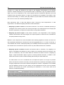
5. For both types of installation a directory to store the scenarios has to be specified (see below).
Restrictions are the same as for the GREAT-ER installation directory.
6. A final dialog enables you to review your settings. Click back to modify your settings, or complete
the installation.
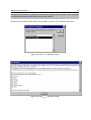
7. The set-up program evaluates the source files and starts to install GREAT-ER. Please note that on
some systems the progress bar reporting the process of installation will not function properly.
8. It is recommended to restart the computer after installation to ensure correct recognition of new
system settings.
9. Finally, you can create a link to the GREAT-ER program in any of the “Start Menu” program groups
or on the desktop. The link target should be as follows:
<ArcView path>\arcview.exe %GHOME%\great-er.apr
where <ArcView path> has to be replaced by the path to your ArcView installation (e.g.
C:\ESRI\AV_GIS30\ARCVIEW\BIN32).
Alternatively, the link or shortcut can point directly to great-er.apr and ArcView will normally be
started automatically.
GREAT-ER User Manual
5
1.3 GREAT-ER AND ArcView
As GREAT-ER is a software system built on top of the GIS ArcView, some familiarisation with the
basic ArcView terminology and functions is recommended. It is outside the scope of this tutorial to
explain all ArcView-specific terms used below. This is especially the case for all the ArcView features
used to create a user-specific presentation of data.
The ArcView handbook gives some tutorials about how to use the basic functions of ArcView. In
addition, the on-line help provides some useful information and the following sections are especially
useful:
■
Introduction to ArcView - This provides a useful introduction to the basics of ArcView, the different
types of data and so-called ‘Documents’.
■
Creating and using maps - This gives a useful description of ‘views’ which display maps and are
therefore the central item of the GREAT-ER user interface.
■
The sections on Displaying a view and Choosing colours and symbols are also useful. Both
contain information on how to work with views and how to modify the presentation of maps and
data.
These basics are sufficient to understand the terminology used in this user manual and to run
simulations with GREAT-ER. If you intend to print or export maps to include simulation results in other
documents or papers, you should read the chapter on Laying out and printing maps. The chapter in
the ArcView handbook with the same name is also helpful.
A basic understanding of the user
interface facilities of ArcView (Menu Bar, Button Bar, Tool Bar) and Windows in general will be useful.
6
ECETOC Special Report No. 16
2. TUTORIAL
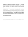
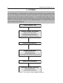
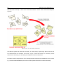
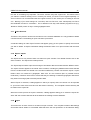
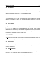
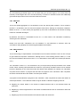
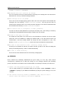
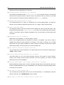
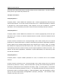
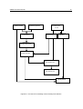
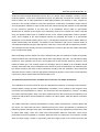
The essential steps to run a first simulation of GREAT-ER are printed within a grey shaded box (like
this one). They represent the minimum contents of the tutorial. A ‘typical’ GREAT-ER session will
generally involve a series of steps as outlined in Figure 2.1. The complete tutorial chapter is seen as a
guided tour through all the main features of GREAT-ER and of the various options available. Finally,
Chapter 3 of this User Manual provides a more detailed description of the different features and
options available within GREAT-ER.
Start GREAT-ER
Create a New Scenario
Specify a Scenario Name
Select Substance and Catchment
Specify Scenario Directory
Specify Number of Monte-Carlo Shots
Run a Simulation
Display Results
Spatial Distribution
Concentration Profile
Add Background Data/Monitoring Results
Save the Scenario
Analyse Model Results
Calculate PECinitial
Calculate PECcatchment
Figure 2.1: Flow Chart of ‘Typical’ GREAT-ER Session
GREAT-ER User Manual
7
2.1 BASIC CONCEPTS
2.1.1 Scenario Concept
The collection of data needed to perform a simulation is called a ’scenario’. Scenarios can be stored
and loaded and thus offer the quick retrieval of certain situations. A unique title for each scenario
assists the search of a specific one in a long list. Additionally, scenarios form the basis of the
exchange of complete simulation data sets (see Export / Import).
A scenario consists of the following data:
1. Title: A unique name for the scenario.
2. Catchment ID: The (identity) ID is the name of the catchment (e.g. Aire). The catchment data
themselves are not part of a scenario. Such data (e.g. river network) are fixed and cannot be
edited.
3. Substance: The whole substance data set is stored within a scenario. The user can safely make
changes to the substance properties for specific simulations without affecting the data stored in
the substance database.
4. Release Data: Although the positions and number of discharge sites within a catchment are not
editable, the attributes of the discharge sites can be modified. For this the set of attributes is stored
with the scenario. In contrast to the substance database, modified data sets can not be written
back to the GREAT-ER catchment database.
5. Modified Flag: The flag is set to true if any element of the scenario has been changed since the
last save and hence the scenario is different to the scenario in the database with the same title.
The flag is displayed in the scenario’s view window title bar (see below).
6. Model Parameter: The complete model parameter data set needed by the GREAT-ER model is
stored within a scenario.
The most important data of a scenario are given in the title bar of the corresponding view window. This
makes the title, catchment ID, substance ID, modified state of scenario/substance and the simulation
state permanently visible and avoids confusion when managing several open scenarios.
2.1.1.1 Scenario Database:
A GREAT-ER installation always has only one scenario database. As mentioned in the section 1.2 on
installation, the basis for the GREAT-ER scenario database is a directory. All scenarios are stored in
8
ECETOC Special Report No. 16
separate sub-directories under this specific GREAT-ER scenario directory. Each sub-directory
contains several tables (with data, such as discharge data, editable by the user) and all additional
settings mentioned above.
Simulation results are also stored in this directory. It is suggested to store further analysis results
under this sub-directory, too. This will increase the transparency of simulation results if all coherent
data are stored in one directory structure. But please note, that in this case deleting a scenario will
also delete any results derived from this scenario!
Given the described scenario database structure it should be noted that the exchange of scenarios
with other GREAT-ER users will not work via scenario database files, but with the export/import
feature described later (see Sections 2.7 and 3.1.8).
2.1.1.2 Active and Open Scenarios
In GREAT-ER you can have many open scenarios, only one of which can be active at one time. The
name of the active scenario is shown in the ArcView title bar. Scenario-related operations always are
performed on the active scenario (e.g. Close Scenario, Edit Data Start Simulation, etc). The view
window that corresponds to the active scenario is usually visible at the front. If a catchment has not yet
been specified, the overview of Europe is visible.
The active scenario can be set by creating a new scenario, selecting a scenario from the scenario
database or by activating the corresponding View window.
2.1.2 Substance Database
The substance database contains all the substance-specific information for any substances that have
been included. The data may include physico-chemical properties, partitioning, degradation, sewage
treatment removal, in-stream removal and market data, depending on what information are available.
It also includes various identification parameters such as the substance name, CAS No. (Chemical
Abstract Service Number) etc. The substance unique ID (key) which is displayed on the screen is
actually made up from the substance name and its CAS No.
It is easy to add new substances or edit substance data as required. However, note that the default
data delivered with GREAT-ER for Boron and LAS have been quality assured and it is not
recommended that these data are modified unless new quality assured data become available.
2.1.3 Expert Mode vs. Easy-To-Use Mode
GREAT-ER offers two modes for the user interface: The expert mode and the easy-to-use mode.
GREAT-ER User Manual
9
’Expert’ in this context requires familiarisation with ArcView. The expert mode gives access to ArcView
operations and commands. This includes the possibilities of undocumented changes or deletion of
basic GREAT-ER data sets. Obviously, this feature provides additional capabilities but also contains a
hidden danger. The user should therefore decide carefully whether to perform operations in the expert
mode or not.
’Easy-to-use’ basically makes it is impossible to harm the system and/or the underlying GREAT-ER
data sets. For undertaking model simulations and viewing the basic results, this mode is sufficient.
2.1.4 Model System
The current version of GREAT-ER comes with a model system covering three sub-models: sewer,
treatment plant and river. There are three complexity modes for each of these sub-models. In the
simplest mode only first-order elimination rates or percentage removal are considered, whereas higher
modes consider elimination processes in more detail.
All of the sub-models are deterministic in principle. However, using the Monte-Carlo method set on
top of these models, results are returned as distributions of concentrations. GREAT-ER delivers
results for all considered geographic objects: sewers (i.e. the influent of a treatment plant), all
treatment plants (effluent) and all river stretches within the catchment under investigation. See the
model description for more details.
Model results are displayed by colouring river stretches on a map, or as concentration profiles along a
river. GREAT-ER provides users with several options to analyse the results and to derive further
values from them. For further details see below in the tutorial and menu description.
2.1.5 Parameter Handling
Depending on the selected models, different parameters will be used to run a simulation. These
parameters are sorted according to their relation to a substance, catchment or model. GREAT-ER
provides several dialogs to enter or modify the parameters.
To display the required parameters according to the selected model’s complexity modes, GREAT-ER
aids users with a colour coding within the dialogs. Parameters colour-coded green are definitely not
used by the current model selection, nevertheless, it is possible to edit these parameters. Black
parameters might be used within the current model selection and if so these need to be specified.
Additionally, GREAT-ER contains a ‘knowledge’ database of parameters to avoid wrong data entries.
Values are compared against two ranges: a warning range and an error range. The warning range
specifies the usual range of a parameter. If an entry exceeds the parameter warning range, a dialog
10
ECETOC Special Report No. 16
will point out this possible mistake. Nevertheless, it is possible to run a simulation with such settings.
In contrast, the error range defines the logical range of a parameter. Values outside this range are
impossible and will lead to errors. If an entry exceeds the error range it is not possible to leave the
dialog until a value within the warning range has been entered. A dialog will give an error message and
hints on the logical range of the parameter. Finally, for better documentation and transparency of
simulation results a separate comment can be entered for each parameter. This comment may
provide additional information for example, about the source of the data, such as quality aspects.
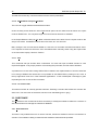
2.2 STARTING GREAT-ER
If you have created a shortcut as mentioned under item 9 of the installation procedure, start GREATER using its icon. Alternatively, start ArcView and select from the menu File the item Open Project...
Browse through the directory tree to the directory of your GREAT-ER installation. Open the project file
great-er.apr.
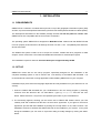
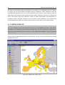
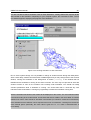
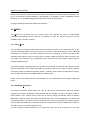
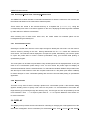
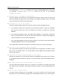
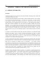
After the start-up GREAT-ER presents the initial screen. It shows a map of Europe and all currently
available catchments.
Figure 2.2: GREAT-ER - initial screen
GREAT-ER User Manual
11
GREAT-ER starts by default in the Easy-to-use mode: the ArcView menu bar is replaced by a specific
GREAT-ER menu bar, the number of buttons and tools is reduced to the set needed for GREAT-ER.
Please note that each menu item (when highlighted) is explained briefly in the bottom left corner of the
ArcView window.
The menu items are ordered according to the usual work flow of a simulation session. Initially you
have to create or select a scenario. The next step is to modify the data. Usually users will simulate a
specific substance with several catchments and may want to use more detailed models if the simple
ones identify issues. Hence the menu bar reflects this order of steps: Substance, Catchment and
Model. The following items enable you to analyse the simulation results and offer various options to
display accessory data or to modify the presentation of data based on additional information.
2.3 SETTING UP A SCENARIO
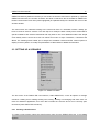
Figure 2.3: GREAT-ER Menu
The first menu of the GREAT-ER user interface, called GREAT-ER, covers all options to manage
scenarios: creating new or loading existing ones, saving, deleting or exchanging with other users. As
usual for Windows applications, this menu also includes the exit item and a list of currently open
documents (here GREAT-ER scenarios).
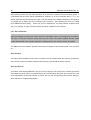
2.3.1 Creating a New Scenario
To create a new scenario, select the ‘New Scenario’ item from the GREAT-ER menu. A new dialog
appears:
12
ECETOC Special Report No. 16
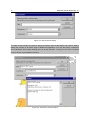
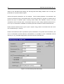
Figure 2.4: New Scenario Dialog
To create a new scenario you have to specify a scenario name at this stage. The name is used to
identify the scenario in all further steps of GREAT-ER application. You may also select a substance
and a catchment at this stage, although this can be left until later. Finally, you can enter a comment
on the scenario to give additional remarks.
Figure 2.5: Scenario Comment Dialog
GREAT-ER User Manual
13
As an example, enter the name GREAT-ER Tutorial and select the substance LAS with the
catchment Aire, then click on OK to leave the New Scenario dialog. You are then asked to specify a
scenario directory name. Enter a non-existent subdirectory name (e.g. tutorial). The directory will
then be created automatically. Each scenario is stored in a separate directory.
Figure 2.6: Scenario Directory Dialog
Finally, to accomplish the generation of scenario data structures, two dialogs will be presented to you
(Model Selection and Catchment Data). Once you are more familiar with the software you may use
these dialogs to speed up the input process for a simulation. Currently you only have to leave them
with "OK". The dialogs will be explained later in this tutorial. Upon leaving these dialogs GREAT-ER
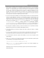
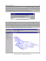
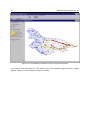
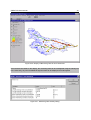
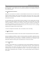
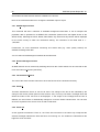
loads the data and displays the selected catchment on the screen (Figure 2.7).
Figure 2.7: Scenario Tutorial with Catchment Aire
14
ECETOC Special Report No. 16
The view now displays the Aire catchment with river network, discharge sites and catchment
boundary, as mentioned in the view's table of contents (to the left of the map). The user can ‘check’
(tick) the different map ‘themes’ in this table to select those required on the display.
The discharge connections are needed because sewage treatment plants may be situated at some
distance from the actual discharge point into the river. Usually the distance is too small to be seen on
the full catchment scale. The site pictures theme is a special theme which is only visible if photos are
available to give users a better impression of the catchment.
The view title bar now gives some summary information about the data displayed: the name of the
scenario, the substance and the catchment. The m in brackets warns users that there are unsaved
changes. It can either appear for the scenario or the substance.
To also see the comments of a scenario, click with the right mouse button on the main display (map).
A dialog with the scenario settings will appear.
Figure 2.8: Scenario Information Dialog
The title bar of the ArcView application now displays the name of the active scenario (see above). This
is helpful if more than one scenario is open and visible on the screen.
At this stage the user can experiment with the some of the tools (e.g. identify, zoom, pan). The
identify tool presents the attributes of selected geographic objects. The user can select a theme from
the table of contents (e.g. discharge sites), click on the ‘i’ icon and then click on a relevant map object
(e.g. a discharge site) to view the various attributes associated with that object. Sometimes, due to
the scale of detail, more than one object might be selected by a click. If this happens, the attributes of
GREAT-ER User Manual
15
each object selected are presented sequentially in separate dialogs. To see them all, click "OK", to
abort "Cancel".
Figure 2.9: Identify Tool Dialog
2.3.2 Needed Inputs
Having now created a new scenario you may use the settings and data loaded from the databases (by
selecting substance and catchment) or modify them.
As mentioned above, GREAT-ER provides three complexity modes for each of the various models.
Obviously, the amount of required data increases with the complexity mode of a model. The GREATER user interface accentuates this by colouring parameter values within the dialogs: Parameters
coloured green are definitely not used in the current model mode selection, whilst those coloured black
might be used.
Please refer to the technical documentation for a detailed description of the model complexity modes
and the required parameters. By default, all sub-models (sewer, waste water treatment and river) are
set to complexity mode one. The parameters needed at this complexity level are mentioned in the
sections below.
16
ECETOC Special Report No. 16
2.3.3 Editing Substance Data
Having selected a substance within the scenario creation, the substance data set is loaded from the
database. To view the data, select Edit Substance from the substance menu.
Figure 2.10: Substance Menu
The substance menu is split into seven categories presented on seven different ‘cards’:
Figure 2.11: Substance Data
GREAT-ER User Manual
17
The various substance data are described briefly below.
identification
The identification card is the first one presented to the user upon entering the substance data. It is
compulsory to give the substance a name; all other parameters which may ease identification are
optional.
physico-chemical properties
In the simplest model modes these data are not required. They are only relevant for the higher modes
as follows :
partitioning
The partition coefficients, if entered here, will override any estimated values calculated from physicochemical properties. In the simplest model modes these data are not required. They are only relevant
for the higher modes.
degradation
In the simplest model modes these data are not required. The parameters are only relevant for the
higher modes.
sewage treatment removal
These data determine how much removal can occur during sewage treatment. In the simplest mode,
GREAT-ER requires a fixed removal efficiency (expressed as the fraction removed) during primary,
activated sludge or trickling filter treatment. All other parameters are related to higher model modes.
Please note that the plant types currently related to the treatment plant in the various catchments
delivered with GREAT-ER always consider a primary settler as the first step in sewage treatment. If
you only have an overall removal fraction (e.g. a combined removal fraction for primary and secondary
treatment) you can set one of them to zero and enter the combined rate in the other.
The sewage treatment card also gives information on another fundamental GREAT-ER concept (if you
have selected the sample LAS substance data set). As described briefly under the basic concepts, the
GREAT-ER models perform a stochastic simulation on top of a deterministic model by the MonteCarlo method. This covers the variations within the catchment’s hydrologic regime but also considers
18
ECETOC Special Report No. 16
other parameters. For most parameters it is possible to specify a distribution. These can be either
normal, logarithmic normal or uniform. Depending on the selected distribution a set of values has to be
entered to describe the distribution. Leaving the distribution dialog you may notice that distributions are
coded by the descriptive values separated by a semicolon. Do not try to specify a distribution by
entering the values directly. Obviously further information is needed to describe a distribution. Always
use the distribution dialog (invoked by the related button) if you want a parameter to be considered as
distributed.
in-stream removal
The in-stream removal card enables you to control the elimination processes within the river. Only an
aggregated first-order elimination rate is needed for the simplest river fate model (mode 1). The other
parameters are only used in higher model modes.
Another GREAT-ER feature is the option to enter a special comment for each value. This is useful to
document the data sources for the various parameters. Try the comment button to obtain further
information on the elimination rate.
market data
The market data card enables you to specify a general consumption value for the substance. This is
slightly different from the Edit Market Data dialog discussed later in this tutorial which enables you to
specify consumption values for selected discharge sites. The current version of GREAT-ER (1.0) does
not allow a distribution to be given for product consumption.
Upon leaving the substance dialog, all substance settings for a first simulation run are made.
2.3.4 Pick Substance and Change Database
The Pick Substance and the Change Database function somewhat differently: The Pick Substance
enables you to copy the substance data from another open scenario. This makes it easier to transfer
specific parameter settings to several scenarios. The Change Database item enables you to change
the database from which substance data are loaded. If you intend to work with a large amount of
substances this feature gives users the opportunity to group substances by classes into different
databases. This increases the transparency of data storage and speeds up data retrieval.
GREAT-ER User Manual
19
2.3.5 Editing Catchment Data
Figure 2.12: Catchment Menu
The catchment data mainly consist of spatial data sets which are not editable within the easy-to-use
mode. The user can only select a new catchment for the currently active scenario. However, it is
possible to select a subset of the current catchment (e.g. the Aire upstream the confluence with the
Calder in the tutorial sample scenario) to focus on the area of interest and to speed up the simulation.
As with the sub-catchment selection, the main items of the catchment menu, Edit Market Data and
Edit Discharge-Site Data, are also managed by ‘tools’.
After selection, the mouse pointer style
changes to identify the new mode. Click on the catchment map to choose the object to be edited.
Edit Market Data
The Edit Market Data dialog enables you to specify site-specific consumption data. To cover industrial
sites, users can enter an additional input into the treatment plant
This input reflects discharges
resulting from the production processes and can be calculated from the production volume. Please
note that the calculation of the fraction of the production volume which will be released is not part of
GREAT-ER but must be calculated beforehand. The input considered here is the mass flow
independently of substance into the treatment plant in [kg/a]. As with the loads from domestic inputs,
the industrial input is subsequently processed by the treatment plant model, if present, for the selected
location.
Figure 2.13: Edit Market Data Dialog
Edit Discharge-Site Data
20
ECETOC Special Report No. 16
Similar to the Edit Market Data dialog, the Discharge-Site Data dialog enables users to modify the
parameters of a specific treatment plant.
Several site-specific parameters can be changed.
These include population, the elimination rate
(used for complexity mode I), the treated fraction of incoming sewage (e.g. bypass or overflow) and in
general the type of treatment plant. Incoming waste waters from separate "sources" are also
considered such as domestic input, non-domestic input (this covers mainly industrial inputs) and runoff. If only an overall value is available for treatment plants this should be entered as domestic flow.
Please note that domestic flow is given in [litre / (capita * day)], whilst non-domestic flow and run-off
3
are considered as [m / second].
Please note furthermore that it is possible to specify a distribution for a general removal efficiency, but
not for a site-specific removal efficiency. Nevertheless, it is possible to have a distributed removal
efficiency for, e.g. activated sludge plants, and a fixed rate for a selected site.
Figure 2.14: Edit Discharge-Site Data Dialog
GREAT-ER User Manual
21
2.4 RUNNING A SIMULATION
Figure 2.15: Model Menu
Having created a scenario and selected the substance and catchment data, the user can then select
the required model parameters and start a simulation.
There are three additional dialog options which the user can select at this stage; Select Model, Edit
Model Parameters and Background Concentration. These are described briefly below:
Select Model
The Select Model dialog also allows the user to select the complexity mode for the different models.
Figure 2.16 shows the options for the river model and similar options exist for the sewer and
wastewater treatment models.
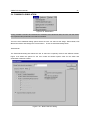
Figure 2.16: Model Selection Dialog
22
ECETOC Special Report No. 16
The text field on the right provides some summary information (hints) on the selected mode. If you
increase complexity modes, it may be necessary to go back to earlier data dialogs to enter additional
parameters. For example, if you need in-sewer removal to be considered, you have to go back to the
substance data dialog to enter a removal rate for sewers. Please note that in-sewer removal is the
only ‘higher’ model in which only one parameter has to be entered. All other ‘higher’ models require a
somewhat larger data set.
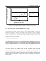
Since GREAT-ER uses the Monte-Carlo method to provide a stochastic approach, the number of
Monte-Carlo shots performed during a simulation also has to be entered within the Model Selection
dialog. As a rule of thumb, the minimum number of shots recommended to obtain a stable simulation
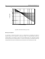
result are as shown in Table 1:
Table 1. Monte-Carlo Simulation
small catchments / simple
large catchments / complex
Csim mean
500
2500
Csim 90%
2500
5000
Edit model Parameters
The Model Parameters dialog allows the user to edit various environmental data and specific
properties of the sewer, wastewater treatment plant and river models. For higher complexity modes, a
useful feature is the "Default" button which can be used to assign pre-selected values to different
parameters. However, please note, that each default value has to be set individually. If you want a set
of all default values to be used for some scenarios this is currently only possible by creating a generic
scenario without a substance or catchment. All further scenarios can then be created from this generic
one and saved to new scenario (use Save As).
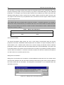
Background concentration
Background Concentrations are included to consider additional loads within the river network which
may be found upstream from the first known discharge. Note that the given value is simply added to
the model results after the simulation. The background concentration is not considered within the
elimination processes.
Figure 2.17: Background Concentration Dialog
GREAT-ER User Manual
23
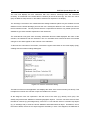
You are now able to start a simulation. Click on Start Simulation. Initially, GREAT-ER ‘exports’ all the
data needed for the simulation. Depending on your computer system, this could take a while. Then a
new window appears, displaying the progress of the simulation:
Figure 2.18: Running simulation on Aire catchment
Due to some system timings it is not possible to change to another window during this initial phase.
After a short delay, window control becomes available again and you may change back to the ArcView
window, running the simulation in the background. A remark [running] in the window title bar
identifies that a simulation is running for the active scenario. The user may now proceed to work with
another scenario or even on the scenario view currently under simulation. You should not modify
scenario parameters while a simulation is running. You should also bear in mind that any user
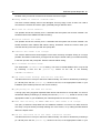
interaction while a simulation is running may significantly increase the simulation running time.
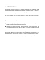
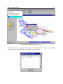
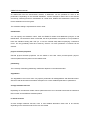
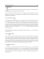
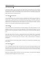
After the simulation has finished, the results will be displayed on the screen. The river stretches will be
coloured according to the model results. A new theme will also be visible in the view's table of contents
entitled Csim mean. Csim stands for simulated concentration (in contrast to monitored concentration);
mean indicates that the different colours represent the mean concentrations resulting from the MonteCarlo method. [More specifically, the mean value is given as Csim,
more detail].
internal
which is described later in
24
ECETOC Special Report No. 16
Figure 2.19: Visualisation of simulation results for the Aire catchment
If you need to abort a simulation for some reason, click on the simulation progress window. A dialog
appears, asking you if the simulation should be continued.
GREAT-ER User Manual
25
Figure 2.20: Process of simulation abortion
If you then select "No", the simulation will be aborted and a report will inform you about the message
sent back from the simulation system to the GREAT-ER user interface:
Figure 2.21: Process of simulation abortion
26
ECETOC Special Report No. 16
The meaning of the menu item Stop Simulation is not the same. This item is a kind of safety guard. If
a simulation fails for some reason (identified for example, by an error message titled rsxnt) you
should select the Stop Simulation menu item. This will change some settings behind the user interface
and enable you to safely save any remaining open scenarios. After selecting this item you should
close GREAT-ER and restart.
Errors may occur if attempting a very large number of Monte-Carlo
shots, for example, or if the numerical solution becomes unstable for some reason.
2.4.1 Save a Scenario
Before proceeding to analyse the model results it is advisable to return to the beginning, the GREATER menu, to save the scenario: select Save from the menu: all scenario settings and the model
results will be saved in the scenario’s directory. A dialog informs you of its successful completion.
The GREAT-ER user interface provides users with two options to save scenario data: save and save
as.
Save Scenario
This option writes all data from the active scenario to the file system under the directory specified for
the scenario, reports successful completion and lets you proceed with the active scenario.
Save Scenario As
This option works slightly differently. First you have to specify a new name for the scenario (scenarios
are identified by their names, so unique names are recommended) and enter any comments to help
future identification of the new scenario. You then click on "OK" and specify a new scenario directory,
which will then be created automatically.
GREAT-ER User Manual
27
Figure 2.22: Save As Dialog
Figure 2.23: Save As Directory Dialog
After using Save Scenario As a message will appear reporting successful completion and reminding
the user of something very important: The active scenario stays the original one. This means that if
you intend to continue working on the scenario just saved, you have to load it again separately. To
avoid confusion it is recommended that the original scenario is also closed prior to loading in the new
one. Warning: If you make changes to a scenario, then use ‘Save As’, then subsequently use ‘Save’
the ORIGINAL scenario is overwritten. This is different to the way other familiar programs work (e.g.
WORD or EXCEL) which is why it is being highlighted here.
28
ECETOC Special Report No. 16
2.5 ANALYSING MODEL RESULTS
Figure 2.24: Analysis Menu
After a model run has been completed, the analysis menu provides various facilities for analysing the
results. Since the results are stored as frequency distributions, it is possible to calculate percentiles of
concentrations (using Calculate River Csim X) for the different river stretches. Alternatively the menu
provides you with features to modify the presentation of results: either by classification or a colour
coded combination of concentrations with flows. The analysis tools most relevant to risk assessment
are the functions to calculate PEC (Predicted Environmental Concentration) values.
Please note that the GREAT-ER analysis tools are designed to analyse distributions of values.
Although it is possible to run a simulation with only one Monte-Carlo shot the analysis functions may
fail if this is attempted.
2.5.1 PEC Calculations
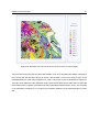
Figure 2.19 shows clearly that GREAT-ER is able to predict the spatial distribution of concentration,
based on real catchment data and known properties of a substance. This is a much more advanced
tool than the generic regional or multi-media approaches.
GREAT-ER also proposes some novel PEC concepts for characterising exposure in river catchments
(Boeije et al, 1999). Several values are provided which are split into two categories: PECinitial and
PECcatchment. Detailed discussion of the underlying concepts is beyond the scope of this user manual,
although a brief description is given below. For further information refer to the technical manual.
PECinitial
This is the spatial aggregation of concentrations in the river directly after emission. This is similar to
the PEClocal as defined in the EU Technical Guidance Documents, although its calculation is different.
GREAT-ER User Manual
29
Based on the Csim, start mean values (see Appendix A), the mean is calculated for all stretches receiving
treated or untreated discharges:
PECinitial =
∑ i =1
n
Csim, start , i
n
Csim, start, i is the concentration at the beginning of river stretch i, directly receiving treated or untreated
waste water emissions.
By definition, the PECinitial is calculated from the Csim, start mean values. This calculation is started by
selecting the item PECinitial.
Please note that PEC calculations are not available if a Sub-catchment is selected.
After the calculation a dialog displays the result alongside additional information.
Figure 2.25: PECinitial calculation results
PECcatchment
This is the average of representative concentrations over the entire catchment. This is a new concept
for geo-referenced exposure assessment, although there is some analogy with the PECregional in the
EU Technical Guidance Documents.
The "most representative" value for the concentration in the stretch is taken as Csim, internal (the average
concentration for the stretch). However, different values could be used and in order to demonstrate
the effect of using different possible definitions, GREAT-ER computes four different PECcatchment
values. These values differ in the set of stretches selected for the calculation and in the weighting of
concentrations.
30
ECETOC Special Report No. 16
All PECcatchment values are defined as the mean of the weighted concentrations of the selected
stretches. Possible selections are (A) all stretches within a catchment or (B) only polluted stretches.
Option (A) is more comparable to the current regional exposure assessment approach (unit world
models) in which all surface waters in a region are considered to be available for the dilution of the
chemical mass loading. In contrast, option (B) considers only the loaded river stretches and allows the
user to focus on the river stretches potentially at risk.
Both approaches have to deal with different issues concerning scale dependencies or data
requirements. The different weighting methods are discussed below:
1. Weighting by stretch volume for both stretch selections. The volume is calculated (assuming a
rectangular cross section) by flow, flow velocity and length. This method places more weight (and
therefore ‘importance’) on large rivers and therefore on high dilution situations.
2. Weighting by stretch length for both stretch selections. The interpretation of this weighting
method is that stretches with equal length are of equal importance. Small rivers are considered to
be equally valuable as large rivers.
Methods 1 and 2 depend on the scale and detail of the underlying digital river network, and the more
that (unpolluted) headwaters are included, the lower the aggregated PECcatchment will be. Conversely, in
a low detailed river network, small (and possibly more valuable) stretches are neglected. Hence these
two methods are most relevant for option B, where only the loaded stretches are considered.
3. Weighting by flow increment considers all stretches within a catchment. The weighting of a
stretch is calculated by the difference of flow in relation to its upstream stretch (two stretches in the
case of a confluence). Thus the values related to stretches are similar to those in weighting by
length. A slight accentuation might be given to receiving stretches because, in addition to the
natural flow increment, these are also artificially influenced by the waste water flow.
The initial stretch of a river is considered with its complete flow (there is no longer an upstream
stretch and thus the increment is the flow). If these stretches are unpolluted, the weighting method
is largely independent of the scale of detail of the digital river network. Regardless of how detailed
rivers are digitised, the flow of a given stretch can be considered as the sum of all its upstream
stretches and therefore the stretch representing the headwaters is of the same value as all
stretches considered separately.
The calculation of PECcatchment can be based on any of the previously derived percentiles of the model
results. When selecting PECcatchment the existence of previously calculated values is first checked
because, depending on the catchment extent and detail of the digitised river network, the calculation
GREAT-ER User Manual
31
may take several minutes. A progress bar will index the progress of the calculation. After completion
the values mentioned above are listed in a small report window:
th
Note that the PECcatchment calculation may be based on mean or 90 percentile Csim values:
Figure 2.26: PECcatchment calculation results
Figure 2.27: PECcatchment calculation results
32
ECETOC Special Report No. 16
2.6 ADDITIONAL DISPLAY OPTIONS
Figure 2.28: Display Menu
The monitoring programmes undertaken in the pilot areas of GREAT-ER form an integral part of the
GREAT-ER project. The data obtained are stored as geo-referenced data (i.e. monitoring sites with
monitoring data as attributes) within the GREAT-ER software. To display these data select Add
Background Data. A dialog will then present a list of all background data available for the active
scenario. Monitoring data will also be available among these.
Figure 2.29: Select Background Data Dialog
The user may select one or more entries. For the purpose of this tutorial select River Monitoring
and STP FE Monitoring, FE stands for Final Effluent and leave the dialog with "OK". Two new
themes are displayed on the view.
GREAT-ER User Manual
33
Figure 2.30: Display of Monitoring Sites for Aire Catchment
Once the data are visible on the display, the monitoring data can be investigated using the identify tool.
In the same way, any other available background data can be displayed and interrogated.
Figure 2.31: Monitoring Data Identify Dialog
34
ECETOC Special Report No. 16
2.7 DATA EXCHANGE
There are two options to exchange simulation results or complete scenarios using GREAT-ER:
■
to share scenarios with other users for further discussion;
■
to generate a report with results for further analysis or inclusion in other documents.
The first option is supported by providing an export / import functionality. Selecting Export, an export
file will be created in the directory of the active scenario. The export file will cover all scenario settings
and additional data derived from the results. Please note that the export / import feature does not
include geographic data such as river network (due to possible licence restrictions). Therefore users
have to ensure that they are working on equal geographic data sets if they want to exchange (and
work with) scenario data. Conversely, an export file can be selected using the Import item and will then
be added as a new scenario to the scenario database.
GREAT-ER provides some features for the second option within the expert mode. The menu item
Report under the GREAT-ER menu can be used to write all scenario data and all results to a specified
file. Specific parts can then be abstracted from this using a common text editor. Another option is to
export a concentration profile for a selected river. By selecting Analysis / Concentration Profile a tool
will be activated, then select a stretch by clicking on the view. Moving downstream the Csim,
internal
values are collected for each stretch. The collection will be displayed in a simple X/Y-profile.
Alternatively there is the option to export the profile data to create a smarter presentation using a
preferred data plotting or spreadsheet program.
It should be mentioned that the full set of simulation results for a scenario are stored under the
scenario directory within the files Csim.dbf (river) and CsimSTP.dbf (treatment plants). Copies of
these files may be used to further analyse the data.
Other options are available under ArcView in the expert mode. The most important function might be
to export the resulting visualisation onto a map by colouring the river stretches. This can be done quite
comfortably using the ArcView layout capabilities.
GREAT-ER User Manual
35
2.8 LIMITATIONS
2.8.1
ArcView
Chart Display
The chart options of ArcView are quite limited. Only 50 data points can be displayed within an X/Y plot
used for the concentration profile along a river. For this reason the profile might not display all
stretches downstream from the selected stretch. To deal with this limitation GREAT-ER provides users
with the Export Profile feature to write the complete stretch set to a file (either plain ASCII or dBase)
for further analysis or more comfortable plotting with the user’s favourite data plotting or spreadsheet
application.
Error Calling Unlink
GREAT-ER combines the data needed for simulations from various tables (which is usual for GIS and
databases in general). ArcView, as the underlying database system, provides a complex sequential
approach for this task. The ‘Error Calling Unlink’ message might occur (usually if a network is
involved) as a result of timing problems while resolving these links (possibly while editing a scenario).
If this error occurs it is recommended to close the scenario and GREAT-ER immediately.
Error in Application
Closing GREAT-ER and therefore ArcView might lead to a cryptic error message caused by ArcView.
This is not an error of GREAT-ER but of ArcView itself. It may also occur if ArcView is opened and is
left again without any further action.
2.8.2 User Interface
Distributions
Several substance-related parameters may not be entered as distributed values but the user interface
does not warn about this directly. Classified according to the dialog's cards these are:
Identification:
Obviously none of the identifications can be entered as distributed.
36
ECETOC Special Report No. 16
Physico-chemical properties:
molar mass
acid versus basic dissociation parameter
Degradation:
anaerobic biodegradation correction factor
anoxic biodegradation correction factor
affinity constant for aerobic / anaerobic
sorbed biodegradation correction factor
temperature correction for biodegradation
In-stream removal:
correction factor for biodegradation in rivers
Sewage treatment:
correction for biodegradation in activated sludge
Market Data:
domestic product consumption.
Note furthermore, that it is possible to specify a distribution for a general elimination rate, but not for a
site-specific elimination rate. Nevertheless, it is possible to have a distributed elimination rate for, e.g.
activated sludge plants, and a fixed rate for a selected site.
Default Values
A set of all default values to be used for some scenarios is currently only possible via a workaround.
Create a generic scenario without a substance or catchment. All further scenarios can be created from
this generic one by saving them as new scenarios (use Save As).
GREAT-ER Analysis Tools
Note that the GREAT-ER analysis tools are designed to analyse distributions of values. Although it is
possible to run a simulation with one Monte-Carlo shot, the analysis functions may fail if this is
GREAT-ER User Manual
37
attempted.
Note that PEC calculations are not available if a sub-catchment is selected.
GREAT-ER Help System
Note that the start-up phase of the help system may take some time to initiate.
Operating System WINDOWS NT 4.0
The operating system GREAT-ER is designed for is WINDOWS NT 4.0. GREAT-ER will not work
properly under W INDOWS 95, although ArcView 3.0 and 3.1 do. Compatibility with W INDOWS 98 was
not tested.
Creating Directories
The feature of directory creation is limited within both the set-up and the GREAT-ER user interface
(e.g. new scenario). The last directory in a path can be created, but new multi-stage directories are
not possible.
2.8.3 Model System
The GREAT-ER simulation system includes detailed sub-models for rivers and activated sludge
treatment plants but only a single percentage removal for sewer and trickling filter treatment plants.
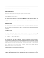
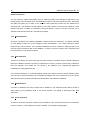
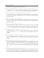
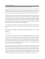
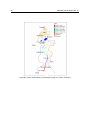
2.9 ADDING A NEW CATCHMENT
The catchment data sets used in GREAT-ER are large and relatively complex structures. All
catchments included in GREAT-ER have to be developed using the GIS system ARC/INFO. However,
in addition to this, several software tools for creating a catchment have also been developed within the
GREAT-ER project which might be useful for future development and inclusion of new catchments.
These software tools are not included with the installation software but are available separately
(please contact ECETOC for further information).
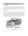
A general overview of the processing steps is given below:
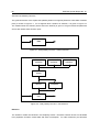
The data required to build a GREAT-ER catchment may exist in several different formats and/or
resolution. This problem is solved by the definition of an intermediate file format. For each data group
a GREAT-ER pre-defined format is given. The required files have to be produced from the original
38
ECETOC Special Report No. 16
raw data, either manually or from some customised software routines which could be developed if
required.
Figure 2.32: Two step data processing
Once all the required data have been converted, the second step is quite simple. Most of the work is
done automatically via ‘makefiles’ and several ‘scripts’. These will execute the necessary format
conversions, data joining, etc. and finally the installation of the new catchment.
All routines used for the production of the currently included catchments are available as source codes
(e.g. for MicroLowFlows datasets) and can be studied (contact ECETOC for further information).
GREAT-ER User Manual
39
3. MENU STRUCTURE
The following sections provide a brief description of all the menu items within GREAT-ER 1.0.
Sections 3.1, 3.2, 3.3 etc correspond to the main menu groups (GREAT-ER, Substance, Catchment,
Model, Analysis and Display). The various sub-sections then describe each of the options within these
groups.
3.1 GREAT-ER
3.1.1
New Scenario
This item is always enabled. A dialog for the specification of a new scenario appears. The minimum
set is to specify a scenario name for identification. The entered name is checked against the existing
scenarios in the scenario database.
Optionally a substance and a catchment may be selected from the related databases. The editing of a
comment is also optional. Leaving the dialog with "Cancel" will abort the creation of a new scenario,
"OK" will bring you to a dialog in which to specify a non-existing directory for the new scenario. It will
be created automatically.
The dialogs Model Selection and Edit Catchment Parameters then appear sequentially. Their
invocation is necessary at this stage to complete the scenario data set. Finally, the new scenario is
made active and the previously active scenario is deactivated.
It is not possible to create a new scenario without a title nor to specify a title already used for another
open scenario. If a catchment has not been selected, the new scenario view will display a map of
Europe.
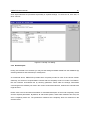
3.1.2 Open Scenario
This item is only enabled if the scenario database contains at least one scenario. The scanning of the
scenario database could take a while if you have already created a number of scenarios.
The dialog that appears is separated into two areas: on the left a list is presented containing all
available scenarios. Select one by click or enter a name in the entry field at the top of the list.
Selecting a scenario by a single click, the fields in the right area display additional information on the
scenario for better identification: substance, catchment, comment and the scenario directory.
40
ECETOC Special Report No. 16
To load the scenario, leave the dialog with "OK" or double-click the selected scenario.
If there is already an open scenario with the same title, the specified one will not be loaded. The one
already open must be closed first.
3.1.3 Edit Scenario
This item is only enabled if there is at least one open scenario. The dialog is the same as under New
Scenario to enable the user to modify the main settings of a scenario in a single dialog: name,
substance, catchment and comment.
If the name has been modified a following dialog will ask you to change the scenario directory. If the
dialog is cancelled or the directory name not changed, the scenario will be kept in the current scenario
directory.
3.1.4 Close Scenario
This item is only enabled if there is at least one open scenario. If the active scenario is not identical to
the scenario in the database with the same title, a dialog will appear giving the option to save the
scenario. Confirmation of saving will also be requested if the active scenario is not in the scenario
database.
However, if Close Scenario is selected, the active scenario will be closed and removed from the list of
open scenarios.
3.1.5 Save Scenario
This item is only enabled if there is at least one open scenario. The active scenario will be saved to the
scenario database. Confirmation is necessary to overwrite a scenario in the database with the same
title.
3.1.6 Save Scenario As
This command is similar to Save Scenario, except that you first have to specify a new title and it is not
checked whether the scenario has been modified. The dialog also provides the option to edit the
scenario comments. Leaving the dialog with "OK" you have to specify a new, nonexisting directory for
the new scenario.
After using Save Scenario As a message will appear reporting successful completion and reminding
GREAT-ER User Manual
41
the user of something very important: The active scenario stays the original one. This means that if
you intend to continue working on the scenario just saved, you have to load it again separately. To
avoid confusion it is recommended that the original scenario is also closed prior to loading in the new
one. Warning: If you make changes to a scenario, then use ‘Save As’, then subsequently use ‘Save’
the ORIGINAL scenario is overwritten. This is different to the way other familiar programs work (e.g.
WORD or EXCEL) which is why it is being highlighted here.
3.1.7 Delete Scenario
This item is only active if at least one scenario is in the scenario database. It is only possible to delete
a closed scenario. The deleting of open scenarios is prevented.
A selection dialog as under Open Scenario will appear giving you the option to specify the scenario
you wish to delete. A simple confirmation dialog will follow if there is no open scenario with the same
title.
3.1.8 Export / Import
The Export item is only active if there is at least one open scenario. The related function acts on the
active scenario. The Import item is always active.
The Export/Import feature helps the exchange of simulation data and results between different users.
The export function applies to the whole active scenario, including any additional documents derived
from the model results and stored in the scenario subdirectory. Please note that the export / import
feature does not include the geographic data such as river network (due to possible licence
restrictions). Therefore users have to ensure that they are working on identical geographic data sets if
they want to exchange (and work with) scenario data.
When "Export" is selected, a dialog appears in which you specify where a scenario is to be exported
to: you have to enter a file name and can also select a directory. The complete scenario directory will
be written to the export file.
When the inverse process of import is selected, a dialog appears asking you to select the export file.
After "OK" the scenario data set will be included in the existing scenario database.
3.1.9 Report
This menu item is active if there is at least one open scenario. The complete scenario data settings
and results will be written to a formatted ASCII-file which the user specifies in a file selection dialog.
42
ECETOC Special Report No. 16
This will also include any comments entered for the various parameters.
3.1.10 Expert Mode / Easy-to-use Mode
The user can ‘toggle’ between these different modes.
Under the Easy-to-use Mode the item Expert Mode option will be visible and will launch the expert
mode of GREAT-ER. The complete range of menus and tools will then be available.
In the Expert Mode the Easy-to-use Mode command sends users back from the expert mode to the
easy-to-use mode. All additional menus and some tools, etc. are removed.
Many changes, such as new themes added to a view are not ‘reversible’ and these will still be active.
If it is required to remove a theme the user must delete them manually, either using the expert mode
or the menu item Display / Remove Themes.
3.1.11 Exit
This command will quit ArcView after confirmation. For each still open modified scenario a save
request will appear. If any major problem occurs during this procedure, the Exit routine will abort.
A possible error screen after closing GREAT-ER is related to the implementation of ArcView itself and
is not a bug of GREAT-ER. Note that it is not possible to exit GREAT-ER by clicking on the ‘cross’ in
the top right-hand corner as in other Windows applications. If this is attempted a message is given
requesting the user to use the Exit command.
3.1.12 n a scenario title
This item list shows all currently opened scenarios. Selecting a scenario title makes this scenario the
active one. The menu item of the active scenario is not selectable (given in grey).
3.2 SUBSTANCE
The Substance menu contains all functions necessary to modify the substance related to a scenario. It
also offers features to manage the substance database.
3.2.1 New Substance
This item is only enabled if there is an active scenario, because a substance must be connected to a
scenario. The substance dialog is raised and the substance data should be specified.
GREAT-ER User Manual
43
As GREAT-ER uses the Monte-Carlo method, a distribution can be specified for most of the
parameters. Depending on the selected distribution, various descriptive values have to be entered.
Conversely, switching back from a distribution to a fixed value, GREAT-ER calculates the mean of the
former distribution as its first guess.
The substance dialog is separated into seven cards:
identification
You can specify the substance name, CAS and EINECS number and additional synonyms to aid
identification. The substance name is essential, the other parameters are optional. It is not possible to
leave the substance dialog with "OK" (i.e. to use the entered data) without specifying a substance
name. The only possibility would be to abort by "Cancel". For each parameter a comment can be
entered.
physico-chemical properties
General physico-chemical properties can be edited on this card. More process-specific physicochemical parameters are placed on the related cards.
partitioning
The necessity of declaring partitioning coefficients depends on the selected model.
degradation
The degradation card covers some very specific parameters for biodegradation and Mooned kinetics.
See the model technical documentation description for a more detailed explanation of parameters.
sewage treatment removal
Depending on the selected models various parameters have to be entered to describe the substance
fate in sewer and the different treatment plants.
in-stream removal
As with sewage treatment removal, more or less detailed elimination rates have to be entered,
depending on the selected mode for the river sub-model
44
ECETOC Special Report No. 16
market information
You can specify a default consumption (kg per capita and year) of the substance assumed for any
discharge site in the simulation area. See Edit Market Data to edit more site-specific data. Cancelling
the dialog will cause you to return to the previous state. Otherwise confirm the new substance by
selecting "OK". The substance is then added to the active scenario. If the previous substance of the
scenario has been modified, a confirmation dialog will appear. If there is an open scenario with a
substance that has the same ID, a hint will be prompted.
3.2.2 Open Substance
This item is enabled if the substance database contains at least one substance. You will be prompted
by a list dialog to select one of the substances from the database. The chosen substance will be
loaded for the active scenario. If the previous substance has been modified, a dialog will ask you to
save the former substance data to the database. If there is an open scenario with a substance that
has the same ID, a hint will be prompted.
3.2.3 Pick Substance
This item is enabled if you have more than one open scenario. It enables users to transfer substance
data from a different scenario. By picking a substance it is easy to create a scenario with a substance
that was perhaps once edited but not stored in the database (e.g. experimental parameter
modifications, invalid parameter set).
If you select a substance, a confirmation dialog will ask if you wish to save the current substance data.
The only way to avoid the replacing of the substance related to the active scenario is to say ‘No’ at this
stage and prevent an existing data set being overwritten in the substance database.
3.2.4 Edit Substance
This item is enabled if the active scenario has a substance. The substance dialog will be shown to
allow editing of any substance data in the active scenario. The dialog is described under New
Substance.
3.2.5 Close Substance
This item is enabled if the active scenario has a substance. This command will remove the substance
from the scenario. If the substance has been modified, a confirmation dialog appear.
GREAT-ER User Manual
45
3.2.6 Save Substance
This item is enabled if there is an active scenario containing a substance. If the substance is not
modified (in relation to the substance data in the substance data base), a hint will be given and nothing
will be done.
Otherwise the substance will be saved to the substance database. If there is a
substance in the database with the same ID, confirmation will be requested.
3.2.7 Delete Substance
This item is enabled if there is at least one substance in the database. A dialog with a list of all
substances in the database will appear. After confirmation the selected substance will be removed
from the database.
3.2.8 Change Database
Change database will offer a file dialog where another database file ( *.odb) can be selected. It is
possible to have many different substance databases. The default database delivered with GREAT-ER
(substance.odb) should only be modified/extended if the new values are quality controlled
(literature/laboratory reference). If you need to work with a large amount of substances, the substance
database concept enables you to store substances in different databases by classes. This increases
the transparency of data storage and speeds up data retrieval.
3.3 CATCHMENT
The Catchment menu provides the catchment-related functions available for a simulation session. The
items in this menu are only available if there is an open scenario.
3.3.1 Select Catchment
A dialog is raised in which you can select a new catchment for the active scenario from the list of
catchments in the database. If the scenario has been modified you will be requested to save it before
selecting a new catchment.
3.3.2 Select Subcatchment
This item enables the selection of a sub-catchment for a simulation, by clicking on the appropriate
river stretches. The new simulation will then only work on all upstream stretches.
If the active scenario already contains simulation results, these will be deleted (after confirmation from
46
ECETOC Special Report No. 16
the user) before the new sub-catchment is selected.
For identification purposes the selected stretch is coloured red and the end of the simulated river
network is marked with a red dot.
This feature reduces the simulation time if only a smaller sub-catchment is of interest. However, it
should be noted that not all of the analysis functions will work on sub-catchment data.
3.3.3 Unselect Subcatchment
This item is only enabled if there is a sub-catchment selection within the active scenario. It will undo a
former sub-catchment setting. If the scenario includes simulation results these will be deleted (after
confirmation from the user) before the entire catchment is once again selected.
3.3.4 Edit Market Data
The Edit Market Data dialog enables you to specify site-specific consumption data. To cover industrial
sites, users can enter an additional input into the treatment plant
This input reflects discharges
resulting from the production processes and can be calculated from the production volume. Please
note that the calculation of the fraction of the production volume which will be released is not part of
GREAT-ER but must be calculated manually beforehand. The input considered here is the mass flow
of substance into the treatment plant in [kg/a]. As with the loads from domestic inputs, the industrial
input is subsequently processed by the treatment plant model, if present, for the selected location.
After leaving the dialog, the market data tool is still active.
3.3.5 Edit Discharge-site Data
Similar to the edit market data dialog, the discharge-site data dialog enables users to modify the
parameters of a specific treatment plant.
Several site-specific parameters can be changed.
These include population, the elimination rate
(used for complexity mode one), the treated fraction of incoming sewage water (e.g. bypass or
overflow) and in general the type of treatment plant. Incoming water from separate "sources" is also
considered such as domestic input, non-domestic use (this covers mainly industrial inputs) and runoff. If only an overall value is available for treatment plants this should be entered as domestic flow.
Please note that domestic flow is given in [litre / (capita * day)], where non-domestic flow and run-off
3
are considered as [m / second].
GREAT-ER User Manual
47
Please note furthermore that it is possible to specify a distribution for a general removal efficiency, but
not for a site-specific removal efficiency. Nevertheless, it is possible to have a distributed removal
efficiency for, e.g. activated sludge plants, and a fixed rate for a selected site.
Leaving the dialog the discharge data tool is still active.
3.4 MODEL
The Model menu provides items for model control. This includes the input of model-related
parameters and settings and the control of a simulation run itself. The items in this menu are only
enabled if there is an open scenario.
3.4.1 Select Model
The text field on the right provides some summary information (hints) on the selected mode. If you
increase complexity modes, it may be necessary to go back to earlier data dialogs to enter additional
parameters. For example, if you need in-sewer removal to be considered, you have to go back to the
substance data dialog to enter a removal rate for sewers. Please note that in-sewer removal is the
only ‘higher’ model in which only one parameter has to be entered. All other ‘higher’ models require a
somewhat larger data set.
The "impose default complexity mode" check button should usually be checked. After reference to the
technical description of the model input tables the (expert) user has the option to specify different
complexity modes for selected geographic objects. However, these options are beyond the scope of
this user manual and are only available within the ‘expert mode’.
Please refer to the model technical documentation for more information on the model's complexity
levels.
3.4.2 Edit Model Parameters
The Model Parameters dialog allows the user to edit various environmental data and specific
properties of the sewer, wastewater treatment plant and river models. For higher complexity modes, a
useful feature is the "Default" button which can be used to assign pre-selected values to different
parameters. However, please note, that each default value has to be set individually. If you want a set
of all default values to be used for some scenarios this is currently only possible by creating a generic
scenario without a substance or catchment. All further scenarios can then be created from this generic
one and saved to new scenario (use Save As).
The set of WWTP-related parameters is so large that it does not fit on a single card. The most
48
ECETOC Special Report No. 16
important parameters are grouped on the card. To edit the complete data set launch the dialog using
the "complete list ..." button. Please refer to the model documentation for more detailed information on
the model’s parameters.
3.4.3 Background Concentration
Background Concentrations are included to consider additional loads within the river network which
might be monitored upstream from the first known discharge. Note that the given value is simply
added to the model results after the simulation. The background concentration is not considered within
the elimination processes.
The concentration has to be entered before running a simulation. The unit is always [mg/L]. After the
simulation the specified background concentration will be added to the model results. If the model
results are displayed in a different unit an automatic conversion will be activated for the background
concentration. Depending on the extent of the catchment, the addition may take some time. Finally, a
remark is added to the scenario’s view title bar (Background Concentration xxx [mg/L]) to
indicate that the background value has been added.
To remove a background concentration, enter a concentration of zero in the dialog.
3.4.4 Start Simulation
This command will start the simulation for the active scenario if all required data have been specified.
Only one simulation is possible at a time for the same catchment, but different catchments can be
simulated simultaneously. In other words, if a simulation is launched for a scenario after some
seconds (due to precise timing of the system) it is possible to proceed with other catchments. More
details about starting a model are given in the tutorial section 2.4 of this user manual.
3.4.5 Stop Simulation
This item is a kind of safety guard. If a simulation fails for some reason (identified for example, by an
error message titled rsxnt) you should select the Stop Simulation menu item. This will change some
settings behind the user interface and enable you to safely save any remaining open scenarios. After
selecting this item you should close GREAT-ER and restart.
Errors may occur if attempting a very
large number of Monte-Carlo shots, for example, or if the numerical solution becomes unstable for
some reason.
GREAT-ER User Manual
49
3.5 ANALYSIS
The Analysis menu provides further functions for the analysis of model results. The menu items are
only enabled if the active scenario contains model results.
Please note that the GREAT-ER analysis tools are designed to analyse distributions of values.
Although it is possible to run a simulation with one Monte-Carlo shot the analysis functions will
probably fail if this is attempted.
3.5.1 Calculate River Csim X
Since GREAT-ER calculates a distribution of concentrations for each stretch (based on the MonteCarlo simulation) this menu item enables users to calculate any percentile from the distribution of Csim,
internal.
The model results are considered as log-normal distributed. After specifying a percentile (the
unit is per cent, hence the specified value must be greater than 0 and less than 100) the values will be
derived per stretch and a new field will be added to the results table. After calculation a new theme is
displayed in the scenarios view, entitled "Csim xx [unit]". The colouring is the same as that used
for the mean values.
The analysis methods mentioned below are possible for either the default Csim, internal mean values or a
derived percentile.
3.5.2 Csim Classes River
After a model run has been completed, the analysis menu provides various facilities for analysing the
results. Since the results are stored as frequency distributions, it is possible to calculate percentiles of
concentrations (using Calculate River Csim X) for the different river stretches. Alternatively the menu
provides you with features to modify the presentation of results: either by classification or a colour
coded combination of concentrations with flows. The analysis tools most relevant to risk assessment
are the functions to calculate PEC values (Predicted Environmental Concentration).
3.5.3 Combine Csim / Flow
The Combine Csim / Flow feature generates a new theme considering both Csim, internal mean and mean
flow. The resulting theme will display the Csim,
internal
mean classification by colour-coding the legend
and the mean flow by stretch width. The user has the option to specify the number of classes per
value. The classes will be formed on the definition: one class for zero values and equal distances for
all other classes.
50
ECETOC Special Report No. 16
The automatically generated legend can be edited using the ArcView legend. You should save this
manually created legend file to the scenario directory to reload on demand because the additionally
generated analysis themes will not be saved with the scenario.
3.5.4 PECinitial
This is the spatial aggregation of concentrations in the river directly after emission. This is similar to
the PEClocal as defined in the EU Technical Guidance Documents, although its calculation is different.
Based on the Csim, start mean values (see Appendix A), the mean is calculated for all stretches receiving
treated or untreated discharges:
By definition, the PECinitial is calculated from the Csim, start mean values. This calculation is started by
selecting the item PECinitial.
Please note that PEC calculations are not available if a sub-catchment is selected. After the
calculation a dialog displays the result alongside additional information.
3.5.5 PECcatchment
This is the average of representative concentrations over the entire catchment. This is a new concept
for geo-referenced exposure assessment, although there is some analogy with the PECregional in the
EU Technical Guidance Documents. PECcatchment is described in some detail in the tutorial (see Section
2.5.1) .
The calculation of PECcatchment can be based on any of the previously derived percentiles of the model
results. When selecting PECcatchment the existence of previously calculated values is first checked
because, depending on the catchment extent and detail of the digitised river network, the calculation
may take several minutes. A progress bar will index the progress of the calculation. After completion
the values mentioned above are listed in a small report window:
A progress bar will indicate the progress of the calculation. After completion the values are listed in a
small report window. Three different results are given based on different weighting methods:
a) weighting by volume based on the subset of loaded stretches and on all stretches within the
catchment;
b) weighting by stretch length based on the subset of loaded stretches and on all stretches within the
catchment;
c) weighting by flow increment based on all stretches within the catchment.
GREAT-ER User Manual
51
3.5.6 Discharge Influent Csim / Discharge Effluent Csim
The GREAT-ER models calculate concentration distributions for both the catchment river network and
the influent and effluent of the catchment’s treatment plants.
These values are stored in the scenario directory in a separate file (CsimSTP.dbf). Using the
corresponding menu item a new theme appears on the view, displaying the discharge sites classified
by either influent or effluent concentration.
After executing one of these menu items once, the model results for treatment plants can be
investigated using the identify tool.
3.5.7 Concentration Profile
Selecting the Profile menu item the cursor shape changes to identify the new mode. You then have to
select a stretch by clicking on the view. Moving downstream the Csim,
internal
values are collected for
each stretch. The collection will be displayed in a simple X/Y-profile. Alternatively you have the option
to export the profile data to create a smarter presentation using your favourite data plotting or
spreadsheet program.
The chart options of ArcView are quite limited. Only 50 data points can be displayed within an X/Y plot
used for the concentration profile along a river. For this reason the profile might not display all
stretches downstream from the selected stretch. To deal with this limitation GREAT-ER provides users
with the Export Profile feature to write the complete stretch set to a file (either plain ASCII or dBase)
for further analysis or more comfortable plotting with the user’s favourite data plotting or spreadsheet
application.
3.5.8 Export Profile
This item is only active if there is already a plotted river concentration profile. A file selection dialog
appears enabling users to specify a file name for the profile. It is recommended to first select the
target directory (by browsing through the directory tree). The file type can then be specified by the file
name extension: use a .txt to export in plain ASCII or .dbf to export a dBase file. See Section 2.7
for more information.
3.6 DISPLAY
The Display menu provides several commands for extending or changing the visual appearance of the
data under investigation. Some commands (Full Catchment Extent, Zoom In, Zoom Out and Identify)
52
ECETOC Special Report No. 16
are standard ArcView features and also available in the tool bar.
None of the commands influence or change the simulation input or output.
3.6.1 Add Background Data
This command will offer a selection of available background information. A set of transport and
population data is provided for all GREAT-ER catchments (derived from the Digital Charts of the
World, DCW). Selecting the DCW, Roads, Rail Roads, City Areas and City Names will be displayed
for the whole country to which the catchments belong. The resolution of the DCW data is 1 :
1,000,000.
Furthermore, for most catchments monitoring and similar data (e.g. water quality classes) are
available as background data.
You can select several background themes at the same time.
3.6.2 Remove Background Data
All DCW themes can be removed by selecting this menu item. Other themes can be removed via the
menu item Remove Themes (see below).
3.6.3 Full Catchment Extent
The view of the active scenario will zoom to show the full size of the catchment boundary.
3.6.4 Zoom In
This item activates the ’Zoom In’ tool for all views. The change of the tool is also indicated by the
change of the mouse pointer (when moved across a view). You may now draw a rectangle which will
define the extent of the new area to be displayed. If the shape of the rectangle and the view is
different, the zoom factor is automatically changed to cover the whole selected area. You can also
click once anywhere in the view to zoom in with a fixed factor.
3.6.5 Zoom Out
As the opposite command of ’Zoom In’, the ’Zoom Out’ tool works in the same way except that the
selected rectangle indicates the area and factor for zooming out. The smaller the selected area the
higher the zoom out factor.
GREAT-ER User Manual
53
3.6.6 Show River Flows
This function creates a copy of the current river network theme and associates the mean river flow
3
([m /s]) with the line thickness (considering the whole river network). The new theme shows a flow
classification with 5 classes. The functionality of the command can also be reproduced by applying the
legend editor (except for copying the theme).
3.6.7 Select Rivernet by Flow
This command allows users to reduce the number of displayed river segments using the criterion of
3
minimum flow. A dialog will ask for the minimum flow value [m /s] to be displayed. Those river
segments with a mean flow lower than this value will then be made invisible. This command is directly
applied to the river network theme of the active scenario (no copy of the theme is created). Hence a
value of ’0’ (or any negative number) means all stretches are displayed.
3.6.8 Identify
This command works in a similar fashion to the ArcView identify tool. By clicking anywhere in a view,
attributes of features of all active themes are displayed in several (subsequent) dialogs. For some
themes more than one data subset is available. The data set can be selected in the upper dialog list
field.
Only those items which are known to GREAT-ER will be listed, together with an appropriate
description and unit. Other items (possibly added in the expert mode) will not be displayed. After
selecting ’OK’, the information about the next theme is shown. ’Cancel’ will stop the subsequent
presentation.
In the expert mode this special Identify dialog is switched off and replaced by the standard ArcView
Identify dialog.
3.6.9 Show Site Pictures
If the corresponding catchment offers site pictures, the mouse pointer will change its shape and the
site pictures theme will become active. Locations at which pictures have been taken are marked with
large dots. Clicking on a dot will launch a window showing the picture of the site in question (this dialog
is a ArcView built-in dialog).
Note that the images are always scaled (see check box at the bottom). This means that the displayed
ratio between width and height may not be the real one.
54
ECETOC Special Report No. 16
One problem is that scaling may be switched on by default on some small desktop size PCs. A picture
exceeding the desktop size leads to the problem that the close window button is inaccessible to the
mouse.
3.6.10 Remove Themes
For all selected themes, a message will appear requesting whether or not to remove the theme from
the view. Exceptions are the standard themes ’River Net’, ’Site Pictures’, ’Discharge Sites’, ’Discharge
Connection’ and ’Catchment Area’. It is not possible to delete these themes via this menu item.
3.7 GREAT-HELP
3.7.1 Contents
The GREAT-ER help system is implemented as a HTML structure similar to the menu structure
description as published in the GREAT-ER manual. After selecting this menu item the default HTMLbrowser of the user’s system will be launched with the table of contents of the on-line help as the
opening window.
Please note that the start-up phase of the help system may take some time to initiate.
3.7.2 About GREAT-ER
This menu item provides basic information on the user interface and the GREAT-ER project itself.
3.7.3 About Model
This menu item provides basic information about the model system.
GREAT-ER User Manual
55
4. GREAT-ER MESSAGES
4.1 CONVENTIONS
We have set up certain typographic conventions to accentuate the meaning of words mentioned in this
manual. The following table describes the main conventions:
Style
Meaning
Serif
Usual text
Italic
Emphasis / menu items / input
CAPITALS
Products / Software
Typewriter
Software output, messages
Typewriter italics
File names, directories
<PATH>
System variables, e.g. PATH
4.2 HINTS
Hints are provided to give information. They appear as messages informing the user that data cannot
be found or some function is not allowed, for example. If these messages appear it does not normally
indicate a serious problem, only that the user needs to make some selection or exit from the particular
option. The following hint messages are given at various times and the additional remarks may help
to clarify what action, if any, is required:
1. No substance database found - creating new.
For some reason the default substance database could not be found. Therefore a new file entitled
substance.odb was created to generate a new default database. You may try to install manually
or to copying another substance database to the default name substance.odb.
2. Sorry, it is not allowed to close this window.
You have tried to close the view of Europe (the GREAT-ER basic view) by the clicking on the
close button ("X") on the window title bar. The resulting process would be similar to the menu item
Exit but is not stable and may cause loss of data. For this reason the action is prevented. Please
use the Exit item to close GREAT-ER.
3. Sorry there is already an open scenario with this title.
It is not allowed to have two open scenarios with the same name. The scenario name is the key to
identifying a scenario and must be unique. Please close the currently open scenario with the name
in question if you want to open the new one.
56
ECETOC Special Report No. 16
4. It is necessary to first save the scenario.
For reasons of stability and data safety it is only allowed to change catchment data for an
unmodified scenario, i.e. a scenario directly saved before changing the catchment data.
5. No substance specified for active scenario.
No substance found for active scenario. As market data and discharge-site data dialogs offer
users the opportunity to overwrite general substance settings by site-specific values, these are
only applicable if a substance has already been selected.
6. A simulation for this scenario seems to be still in progress.
This is a typical hint: currently not available, the function can be executed some time later because
it is not possible to run more than one simulation at a time for a scenario.
7. This selection tool has to be applied to the active scenario view.
You have clicked on the view with the European overview while the Sub-catchment selection tool
was active. The message appears, because it is not possible to select a stretch from the overview.
4.3 WARNINGS
Warnings are given if something has gone wrong. These are different to errors in the sense that they
do not cause a loss of data and may be resolved with the use of the technical documentation.
1. Environment variable <GHOME> not set.
This environment variable (specifying the GREAT-ER home directory) is established by the set-up
program. However, if this error occurs it means it is now missing (maybe deleted manually).
Following the warning a dialog will be given to enable you to specify the home directory for the
current GREAT-ER session. However, it is recommended to set the variable permanently with the
system settings.
2. Environment variable <GSCENARIOS> not set.
Although this environment variable needed by GREAT-ER (specifying the GREAT-ER scenario
directory) is set by the set-up program, it is now missing (maybe deleted manually). A following
dialog enables you to specify the home directory for the current GREAT-ER session but it is
recommended to set the variable permanently with the system settings.
3. No unit information available. Unit is set to [mg/L]. Please check your
system / scenario parameters!
For some reason the automatic unit conversion has failed. The simulator output is [mg/L] so it is
assumed that the loaded data is in this unit. Please check this assumption. This message also
appears when no release of the substance has been specified (e.g. a catchment with only industrial
discharges and no site-specific release).
GREAT-ER User Manual
57
4. GREAT-ER menu not found.
The GREAT-ER menu structure seems to be corrupt. This can happen by modifying the structure
in the Expert Mode. A rough solution is to leave GREAT-ER without saving anything. If you want to
save your scenario data you have to restore the menu structure: See the ArcView manual for
customising a project. Check the menus for the View Doc. Rename the one which contains the
usual GREAT-ER commands back to "&GREAT-ER".
5. Exit item not found.
The GREAT-ER menu structure seems to be corrupted. This could happen by modifying the
structure in the Expert Mode. A rough solution is to leave GREAT-ER. You may save your
scenarios before leaving. An alternative is to restore the menu structure: See the ArcView manual
for customising a project. Look in the GREAT-ER menu for the ‘View Doc’. Scan through the menu
items and find the item with the click script Exit GREAT-ER.ave Rename it to "Exit".
6. Not able to fully delete the scenario. The scenario may now be invalid.
Possible reason is access violation.
Because of some file access limitations, GREAT-ER was not able to delete the scenario data
completely. One of the files in the directory may be being accessed by another program. Please
close the file and remove remaining scenario data by deleting the scenario directory manually.
7. Creation of export file xxx failed.
Due to some access limitations, the automatic generation of the export file is not possible. You
might try to change the access restrictions and export again or to export the scenario manually: as
all scenario data are stored in the related directory under the GREAT-ER scenario directory the
export file is a zip archive of this subdirectory. You can create this archive with you favourite zip
tool.
8. Importing of file xxx failed.
Because of some access limitations the automatic unpacking of the export file is not possible. You
might try to change the access restrictions and import again or to import the scenario manually: as
all scenario data are stored in the related directory under the GREAT-ER scenario directory the
export file is a zip archive of this subdirectory. You can unpack this archive with you favourite unzip
tool to the scenario directory.
9. Neither CAS nor Name specified.
The last changes have been lost because the data set has no CAS number or name, which are the
minimum requirements to identify a substance data set.
10. Not able to open database - keeping previous.
Two reasons are possible here: Either, due to access limitations, the database is not accessible or
the database has somehow been deleted, which should not normally be the case.
58
ECETOC Special Report No. 16
11. River network theme missing. Function not available.
The river network theme cannot be found, which means it is no longer a theme of the active view or
it has been renamed. The easy-to-use way to fix both is to save and close the scenario and reopen
it. When using the expert mode the problem can be solved by adding the river network theme to
the active view or by renaming it to "River Net" in the Theme/Properties window.
12. Discharge sites theme missing. Function not available.
The discharge site theme can not found, which means it is no longer a theme of the active view or
it was renamed. The easy-to-use mode way to fix both is to save and close the scenario and
reopen it. When using the expert mode the problem can be solved by adding the rivernet theme to
the active view or by renaming it again to "River Net" in the Theme/Properties window.
13. Discharge table is not editable.
This is due to access restrictions. To enable the discharge table to become editable the access
rights need to be changed.
14. xxx : can not be opened for writing.
This is due to access restrictions and can be solved by changing them. This "warning" involves no
loss of data.
15. The
table
of
simulation
results
is
not
editable.
Calculation
of
background concentration xxx aborted.
This is due to access restrictions and can be solved by changing them.
16. Csim theme feature table has errors.
One of the fields QMean, Reallength, VMean or PECintMean is missing in the theme’s feature
table, probably due to the fields having been renamed manually. This edit need to be undone. A
second possibility may be that the field is hidden. This can be fixed by ‘unhiding’ the field within the
Expert mode.
17. The table of simulation results is not editable. Calculation of xxxpercentile aborted.
This is due to access restrictions and can be solved by changing them.
18. The
theme’s
legend
is
not
as
required
for
PEC’s.
Profile
plotting
aborted.
The current legend classification is based on more than one field. This is not possible for profile
plotting. Switch to the one field which should be used for plotting the profile.
19. Background data table not found.
The table that contains information about additional background data can not be found. This
indicates that the catchment installation routine did not work correctly or the table has been deleted
or renamed manually. The file backgroundlst.dbf needs to be in the directory
GREAT-ER User Manual
59
%GHOME%\catchments\<CATCHMENT>.
20. Background data list could not be created.
This is an internal AVENUE error which should not normally occur. Nothing has to be done and no
data will be lost. Just try to reload the background data.
21. DCW coverage can not be opened.
One or more of the coverages pppoly, pppoint, rdline, rrline can not be opened. Check whether the
coverages are in the directory %GHOME%\overview\<COUNTRY>. This may be the case if a
scenario with a catchment from a new country has been included. In this case the DCW data need
to be included in the directory %GHOME%\overview\<COUNTRY>.
22. Your scenario data is incomplete: no model parameters.
You have to edit the model parameters to specify all necessary ones, This warning is caused by
cancelling the model parameter dialog during the creation of a new scenario.
23. Picture of xxx (yyy) not found.
The image file of the picture can not be found. It may be deleted or renamed. Go into the expert
mode and check the database by loading the attribute table of the Site Pictures theme (via
Themes/Table...) and then looking whether the image file name corresponds to a file in the
directory %GHOME%\graphics\sitepics. If there are some inconsistencies, eliminate them.
24. Not able to save scenario in xxx - directory already exists.
As saving is not possible to a directory of another scenario, go back to the "Save As" dialog and
specify a nonexisting directory. It will be created automatically.
25. Not able to create directory
This is due to access restrictions and can be solved by changing them.
4.4 ERRORS
Errors indicate that something fundamental has gone wrong. An error may cause serious
consequences, especially loss of data. But usually an error message indicates that something
previous has failed or was deleted. Hence a GREAT-ER error message is caused by an earlier error.
1. Banner file xxx/graphics/greater.gif not found!
This is usually caused by an impossible setting for the system variable %GHOME%. Check if
%GHOME% is pointing to your GREAT-ER installation (by using the system settings); if not, set it
correctly.
2. The scenario directory named by GSCENARIOS (xxx) does not exist!
Please create the directory and restart GREAT-ER.
60
ECETOC Special Report No. 16
Create the directory pointed to by %GSCENARIOS% (as indicated in the system settings) and
restart GREAT-ER.
3. Cannot get file xxx!
Without this file the execution of GREAT-ER is not possible. The problem may in some cases be
solved by changing access restrictions. Otherwise the file can be read from the CD by extracting it
from the file greater.zip on the CD into the directory %GHOME%\ave. This message also arises
when the set-up has been performed manually using an old version of ZIP that cuts the filenames
to the old 8.3 convention. In this case, use the set-up program (recommended) or a newer version
of ZIP.
4. Cannot get script load procedure! This makes it impossible to launch
GREAT-ER.
This indicates that the script ReloadScript.ave is not loadable. The problem may in some
cases be solved by changing access restrictions. Otherwise ReloadScript.ave can be read
from the CD by extracting it from the file greater.zip on the CD into the directory
%GHOME%\ave. This message also arises when the set-up has been performed manually using an
old version of ZIP that cuts the filenames to the old 8.3 convention. In this case, use the set-up
program (recommended) or a newer version of ZIP.
5. Cannot compile load procedure! This makes it impossible to launch GREATER.
This indicates that the script has errors, i.e. it has somehow been modified. It needs to be
reinstalled by either reinstalling the whole GREAT-ER software or by installing, i.e. extracting, only
the scripts that contain errors from the file greater.zip on the CD into the directory
%GHOME%\ave.
6. Error occurred opening script file xxx!
The script could not be opened. The problem may in some cases be solved by changing access
restrictions. Otherwise ReloadScript.ave can be read from the CD by extracting it from the file
greater.zip on the CD into the directory %GHOME%\ave. This message also arises when the
set-up has been performed manually using an old version of ZIP that cuts the filenames to the old
8.3 convention. In this case, use the set-up program (recommended) or a newer version of ZIP.
7. Error occurred compiling script xxx!
This indicates that the script has errors, i.e. it has somehow been modified. It needs to be
reinstalled by either reinstalling the whole GREAT-ER software or by installing, i.e. extracting, only
the scripts that contain errors from the file greater.zip on the CD into the directory
%GHOME%\ave.
8. No catchment database found!
GREAT-ER User Manual
61
The essential file catchments.dbf is missing. You have to reinstall GREAT-ER or only the file
by extracting it from
the file greater.zip, stored on the CD, to
the
directory
%GHOME%\catchments.
9. Internal Error: StretchID field missing!
The field to identify river stretches in the simulation result table is missing. Either the field name
has been changed manually (it has to be ’stretchid’) or the data is seriously corrupt. You should
start a new simulation using the same parameters.
10. Catchment CCC can not be opened!
The basic catchment data or parts of it are missing. There are three possibilities for this:
a. You imported a scenario for a catchment you do not have the data for. Check your installation
and contact the party from which you obtained the scenario to update your catchment
database;
b. Your catchment database (under your GREAT-ER installation in the directory ’catchments’
and its sub-directories) has the wrong read access restrictions. Change these settings by
yourself if possible or ask your system administrator;
c.
Your catchment database has been seriously corrupted. Try to restore the catchment data by
reinstalling GREAT-ER over your existing installation.
The essential basic catchment coverages are: catchbound, disch_river, rivernet, discharges.
11. Not able to get information about scenario!
The communication between this dialog and the GREAT-ER core application has failed. ArcView
has run into an unstable mode. It is recommended to leave GREAT-ER immediately without
saving and to restart it.
12. Substance not found! Database seems to be corrupt!
Although the substance you have selected is listed in the database there seems to be no data for
it. This suggests that the substance’s data set, or more generally the substance database itself, is
damaged.
13. The result theme data structure seems to be corrupt!
The result theme data structure seems to be corrupted. You should try to recreate the scenario
and restart the same simulation. If the problem should occur again, one of the needed idfields are
missing ...
14. Can not open ’scenario.odb’!
The basic scenario settings are not accessible. This may be caused by the wrong access
restrictions, which can be fixed by changing them to read/write permission, or by a loss of data. In
62
ECETOC Special Report No. 16
the latter case you need to reconstruct the scenario and save it again.
15. Wrong number of items in ’scenario.odb’!
The basic scenario settings seem to be damaged. This may imply a loss of data. You need to
reconstruct the scenario and save it again, preferably using a different name.
16. No view for active scenario!
This problem should not normally occur. It indicates that the system has become unstable. You
should therefore leave GREAT-ER without saving.
17. Active scenario not found!
This problem should not normally occur. It indicates that the system has become unstable. You
should therefore leave GREAT-ER without saving. Simulation results are stored under your
scenario directory in the files ’pec.dbf’ and ’pecstp.dbf’.
18. Scenario data seems to be corrupt!
The scenario data structure would appear to have been seriously corrupted. Saving is no longer
possible. Simulation results which you might want to keep are stored under your scenario directory
in the files ’pec.dbf’ and ’pecstp.dbf’. Exit the scenario without saving.
19. No catchment database found!
The essential file catchments.dbf is missing. You have to reinstall GREAT-ER or only the file
by extracting it from
the file greater.zip, stored on the CD, to
the
directory
%GHOME%\catchments.
20. xxx table fields missing! Function not available.
The table seems to be corrupt or has been edited manually. You have to reinstall it by extracting it
(a *.dbf file) from the file greater.zip, stored on the CD, to the appropriate location in your
installation (see Table/Properties for the correct location).
21. QueryString for xxx table has errors!
A wrong query string suggests impossible field names and therefore a corrupt table. You have to
reinstall the table by extracting it (a *.dbf file) from the file greater.zip, stored on the CD, to the
appropriate location in your installation (see Table/Properties for the correct location).
22. More than one entry for WWTP! WWTP data table seems to be corrupt.
The query to obtain the wwtp data from the database resulted in more than one data record for
one wwtp. It may be fixed by manually deleting one of the entries, i.e. by editing the table WWTP
data in the Expert mode.
23. Can not find field fff in xxx table! Simulation aborted.
The table seems to be corrupt or has been edited manually. You have to reinstall it by extracting it
(a *.dbf file) from the file greater.zip, stored on the CD, to the appropriate location in your
GREAT-ER User Manual
63
installation (see Table/Properties for the correct location).
24. Required parameter ppp not found in xxx dataset! Simulation aborted.
The dataset seems to be corrupt or has been edited manually. You have to reinstall it by extracting
it from the file greater.zip, stored on the CD, to the appropriate location in your installation.
25. Simulation results: the Csim xxx field was not found!
This error should never occur. It suggests that the simulation table has an incorrect structure. If
this happens, just delete these simulation results, save the scenario and restart GREAT-ER to
repeat your simulation.
26. Csim theme feature table not found!
This error should never occur. It suggests that the simulation table has an incorrect structure. If
this happens, just delete these simulation results, save the scenario and restart GREAT-ER to
repeat your simulation.
27. Can not find table with STP Csims!
The scenario data structure seems to be corrupt. This might have been caused by a loss of data
or by renaming the result tables. You can check this by looking to see whether the file
CsimSTP.dbf is in the scenario’s directory. The easiest way to fix this is to repeat the simulation.
28. Discharge record not found!
The database seems to be corrupt or has been changed manually. You have to reinstall it by
extracting it from the file greater.zip, stored on the CD, to the appropriate location in your
installation.
29. Background data table seems to be corrupt!
One of the essential fields "Name", "MapName", "Type", "Legend" has not been found. This
means the installation is either corrupt or was changed manually. A reinstallation from the CD is
necessary.
30. Necessary script for data set xxx not found!
The background data table indicates a special script to be used for displaying the selected data.
The script is not loadable, i.e the selected background data can not be displayed. The necessary
script is given in the file backgroundlst.dbf in the catchment-specific subdirectory of the
overview directory. The table can be added in the Expert mode to look (and then search for) the
script.
31. Error occurred compiling display script xxx!
The background data table indicates a special script to be used for displaying the selected data.
The script seems to have some errors hence compiling (which is previous to executing) has failed.
This makes it impossible to visualise the selected background data automatically. The file must be
64
ECETOC Special Report No. 16
edited by an AVENUE programmer to fix the error.
32. Background data information not complete!
The background information table backgroundlst.dbf is not complete. Refer to the technical
manual for the required structure, and then look to see whether this is the same for the table
which is stored in the catchment-specific subdirectory of the overview directory.
33. Unsupported background data format!
The background data is of a type not considered in the current implementation. The data can
therefore not be displayed. Supported types are point, arc, polygon, shape, grid and image.
34. Cannot make xxx theme!
The background theme could not be loaded. Check whether the name and the path given in the
background information table backgroundlst.dbf are valid. If not, change them (in the Expertmode) or, more easily, make a complete reinstallation. First, check whether you have read access
to the data.
35. Background data not loadable!
ODB: either access problems, or a file is missing or corrupt.
Parts of the background data you selected are missing or unreadable. First check if data is
available and change access restrictions if necessary. If the data is missing, try to reinstall
GREAT-ER over your existing installation to restore the data. If the data is not part of the original
GREAT-ER package, contact the party you received the data from.
36. xxx table not editable! Analysis aborted.
This is usually due to access restrictions. You require write access in the directory named by your
<TEMP> system variable.
37. Picture theme missing! Function not available.
The picture theme is not in the scenario dictionary structure. This implies a corrupt scenario.
Create a new scenario using the same catchment. If the error persists, you need to reinstall
GREAT-ER over your old installation.
38. Picture theme seems to be corrupt! Function not available.
Essential fields are missing, due to corrupt or manually changed data. If the catchment was part of
the CD, reinstall GREAT-ER over your old installation. If not, contact the catchment’s data provider
to enquire how to proceed.
39. Not able to save scenario.odb
This is caused by a missing write access in your scenario directory, i.e. a subdirectory under the
directory named by your <GSCENARIOS> system variable.
40. Not able to write xxx. Scenario may be corrupt now!
GREAT-ER User Manual
65
This is caused by a missing write access. It may have caused a loss of data.
41. No subcatchment selected in the active scenario.
Although the flags report a sub-catchment for the active scenario the required information can not
be found in the data structures. This suggests the scenario data are damaged. Try to recreate the
scenario using a new name.
66
ECETOC Special Report No. 16
APPENDIX A. CHEMICAL FATE SIMULATOR AND MODELS
A.1 CHEMICAL FATE SIMULATOR
Description
A detailed description of the geo-referenced chemical fate simulation methodology used in GREAT-ER
was published in Boeije et al. (1997).
To deal with statistically distributed inputs and outputs, a hybrid simulation approach is used, involving
both stochastic and deterministic techniques. The model core is deterministic. By means of Monte
Carlo simulation, a stochastic layer is added on top of this core. A large number of ‘shots’, which are
discrete samples from the distributed data set, are generated. For each distributed input parameter,
there exists a discrete counterpart in the ‘shot’, which was sampled at random from the input
distribution. For each of these ‘shots’, the deterministic model is called, which contains a mechanistic
description of the considered processes in the rivers and in the waste water drainage areas. Process
rates are derived from knowledge about chemical properties and process specifics.
Finally, the
(discrete) results from each ‘shot’ are statistically analyzed, to obtain distributed results as simulation
output.
For reasons of model and data set simplicity and computation performance, only steady-state model
formulations are applied. Hence, a number of fundamental assumptions are made: (1) constant
chemical emissions: diurnal patterns in product and water consumption are disregarded, as well as
variations between different days of the week; (2) constant flows within each steady-state model
calculation run; (3) constant environmental properties.
To allow a straightforward mass-balancing approach, all determinands (chemical levels, water flows)
are expressed as fluxes. Chemical mass fluxes Φ (mass/time) are applied to describe chemical loads.
Water flows are expressed as volumetric fluxes Q (volume/time).
In the models, chemical
concentrations C (mass/volume) are not used, because they are not independent of water flows, and
they do not describe chemical transport. Chemical mass fluxes, on the other hand, are independent of
dilution or flow (unless this dependency is implicitly included in the models which are used to calculate
chemical mass fluxes). When concentrations are explicitly required, they are derived from the
chemical mass fluxes and the hydrological volumetric fluxes: C = Φ / Q.
Simulations can be performed for different scenarios (i.e., evaluations of different chemicals and
chemical consumption patterns).
scenario-dependent data set.
The simulation input consists of a scenario-independent and a
These data are expressed as statistical frequency distributions,
incorporating seasonality and parameter uncertainty. Environmental characteristics are constant, and
hence non-scenario-dependent. These include the river network structure, flow and flow velocity
GREAT-ER User Manual
67
distributions, discharge point locations, treatment plant information, emission data, properties of
sewers and small surface waters, etc. Chemical-specific information is scenario-dependent: chemical
properties (i.e., biological, chemical and physical properties, specific process rates,...), and chemical
market data (i.e., per capita product consumption rates). Market data are geo-referenced in the same
way as the waste water information (i.e., related to waste water discharge points).
The simulation input data are expressed as statistical frequency distributions. This allows to include
both seasonality effects and parameter variability and/or uncertainty into the simulation input. For river
flows and flow velocities, the lognormal distribution is used (after NRA, 1995).
For hydrological
th
information this distribution is described by the mean and the 5 percentile. In the case of flows, there
th
is a 95% probability that the 5 percentile low flow (also referred to as Q95) is exceeded: P(Q>Q95) =
0.95.
The simulation results are frequency distributions of chemical concentrations, incorporating temporal
variability. For risk assessment purposes, these can be expressed as lognormal distributions, defined
th
by their mean and 95 percentile values. Predicted concentrations are geo-referenced in the same
way as the input data set: river concentrations are associated with a river network structure, and waste
water drainage area concentrations are associated with discharge points.
Within one location, a
further differentiation is made between the maximal predicted concentrations (i.e., upon discharge),
the minimal predicted concentrations (i.e., after degradation processes), and an ‘internal’ average
value. For the calculation of the latter, specific algorithms have to be provided in the deterministic
models.
Simulation Output
The output of a simulation consists of a geo-referenced set of predicted concentrations in the aquatic
environment. For each river stretch, the following results are obtained:
■
RIVER
CSIM,start
predicted concentration at the beginning of the stretch
CSIM,internal
average predicted concentration in the entire stretch
CSIM,end
predicted concentration at the end of the stretch
■
WWTP
(only if a waste water emission occurs in the considered stretch)
CSIM,influent
predicted WWTP influent concentration
CSIM,effluent
predicted WWTP effluent concentration
A.2 CHEMICAL FATE MODELS
Three ‘complexity modes’ are available. At higher ‘complexity modes’, more detailed models are
used.
68
ECETOC Special Report No. 16
General Fate Pathway Structure
The general structure of the aquatic fate pathway within one segment (without a waste water emission
point) is shown in Figure A.1. For a segment which contains an emission, it is given in Figure A.2.
The treated sewer flow fraction (which enters the WWTP) is given in the geo-referenced parameter
set for each waste water emission point.
river
Figure A.1: Fate pathway structure - without emission
domestic
emission
non-domestic
emission
runoff
emission
sewer
WWTP
untreated
river
Figure A.2: Fate pathway structure - with emission
Emission
The emission models are identical in all complexity modes. Domestic emission fluxes are calculated
from population numbers, market data and water consumption. For other emissions (non-domestic
GREAT-ER User Manual
69
and runoff), the chemical mass fluxes are taken directly from the emission data. The flows are taken
directly from the geo-referenced parameter set.
Transport / Conversion
Complexity Mode 1
Complexity Mode 1 allows GREAT-ER simulations with a minimal geographically referenced and
chemical input data set. No in-sewer removal is assumed to occur. Chemical elimination in a WWTP
is described by a fixed removal efficiency, which depends on the type of treatment.
Chemical
elimination in rivers is described by first-order in-stream removal, assuming a fixed rate coefficient.
Complexity Mode 2
Complexity Mode 2 allows GREAT-ER simulations with a minimal geographically referenced input
data set for rivers. However, for WWTPs a detailed data set is needed, as well as a detailed chemical
parameters set.
In-sewer removal is assumed to be a fixed percentage, and is taken directly from the chemical
parameter set. Chemical elimination in a WWTP is described by mechanistic mathematical models for
primary settling and for activated sludge (derived from SimpleTreat 3.0, Struijs, 1996). For trickling
filter treatment, a simple percent removal model is used. Like in mode 1, chemical elimination in rivers
is described by first-order in-stream removal, but here sorption equilibrium is taken into account. The
different sub-processes (degradation, volatilization, sorption-sedimentation) are dealt with by fixed
removal rate coefficients.
Complexity Mode 3
Complexity Mode 3 requires detailed parameters for rivers, for WWTPs and for the simulated
chemical.
In-sewer removal is assumed to be a fixed percentage, and is taken directly from the chemical
parameter set (identical to mode 2). Chemical elimination in primary and activated sludge WWTPs is
described by models derived from SimpleTreat 3.0 (Struijs, 1996). For trickling filters, it is described
by a fixed removal efficiency (identical to mode 1). The separated individual river fate processes are
described by means of mechanistic models (cf. Trapp and Matthies, 1996), and degradation is further
split up into three sub-processes (biodegradation, hydrolysis, photolysis).
solubility is also taken into account.
The chemical’s water
70
ECETOC Special Report No. 16
APPENDIX B. HYDROLOGICAL MODELLING WITHIN GREAT-ER
B.1 INTRODUCTION
Estimates of the magnitude and variability of river flow and flow velocities at ungauged river reaches
are an essential component of GREAT-ER. There is a considerable variation in river flow behaviour
across Europe over both space and time. The seasonal flow regime of a Mediterranean catchment,
with its winter high flows, dry periods in summer and frequent flash floods, is very different from that of
an English lowland chalk stream, where flows show little variation over the year. Both have a very
different seasonal regime from a catchment in the Alps where maximum flows follow the spring
snowmelt. At the broadest European scale, river flow regimes are dependent on rainfall, temperature
and evaporation. At a finer scale, the detailed effects of a particular climate on river flows are
controlled by the physical properties of the catchment. River flow regimes are also affected directly
and indirectly by human activities such as reservoir impoundment, abstraction of water and effluent
discharges. Taking the UK as an example of a member state with a mature river gauging network,
less than one percent of reaches mapped at a scale of 1:50,000 are gauged and, furthermore, less
than 20% of gauged catchments can be regarded as being natural. The development and application
of steady state hydrological models by the Institute of Hydrology for predicting flow statistics and flow
velocities at ungauged river reaches are presented in this appendix. Central to the models is the use
of a digital river network and thematic digital grids of relevant catchment characteristics. The structure
of the digital river network facilitates the estimation of catchment boundaries, catchment
characteristics and indexing of artificial influences (abstractions, discharges and impounding
reservoirs), the influence of which are incorporated into the model. The flow models are incorporated
into an Institute of Hydrology PC based software product which has been in operational use since
1991 within all of the environmental protection agencies within the UK.
The steady state hydrological models applied within the UK Pilot Study catchments to generate reach
based estimates of both the natural and artificially influenced flow regimes using catchment
characteristic based regional flow models are also described. The use of this type of model is
recommended by the Institute of Hydrology for use within GREAT-ER. The models are intensive in
terms of the spatial data and sample set of gauged data required, but once developed they can be
applied within any catchment described by the spatial data, in this case the UK.
Section three describes the hydrological model developed for the Lambro pilot study catchment. In this
case traditional hydrological techniques were used to harmonise the gauged data associated with five
gauged locations within the catchment. These data were used to statistically describe the flow
regimes. The flow statistics were then extrapolated to the ungauged river sites within the network
using the river network based modelling framework as that used in the UK Pilot study catchments.
GREAT-ER User Manual
71
B.2 THE UK MODELS AND THE RIVER NETWORK BASED MODEL
FRAMEWORK
The first major UK study of the relationships between low flow regimes and physiographic and climatic
catchment characteristics and associated hydrological models was published by the Institute of
Hydrology as the 1980 Low Flow Studies Report (NERC, 1980). The techniques for estimating annual
and monthly low flow statistics are summarised in the following sections.
Annual Flow Statistics
The models used to estimate annual flow statistics are based on a simple conceptual water balance
model for estimating mean flow (MF), and a statistical multivariate model for estimating the Q95
statistic (i.e. the flow equalled or exceeded for 95% of the time) from the hydrological response of soil
types. The mean and Q95 flow statistics estimated from catchment characteristics are used to
determine the flow duration curve (FDC) for an ungauged catchment. The overall estimation
procedure is presented as a flow diagram in Figure B.1. The individual stages are briefly summarised
here. A more detailed description of the models is presented in Gustard et al (1992).
DEFINE CATCHMENT BOUNDARY
AND OVERLAY ONTO MAPS TO
DETERMINE:
FRACTIONAL EXTENT
OF SOIL CLASSES
CALCULATE STANDARDISED Q95
USING A REGRESSION MODEL
RELATING Q95 TO SOIL CLASS
AVERAGE ANNUAL
RAINFALL
ESTIMATE
CATCHMENT AREA
AVERAGE ANNUAL
POTENTIAL EVAPORATION
ESTIMATE MEAN FLOW USING
SIMPLE WATER BALANCE MODEL
IDENTIFY STANDARDISED
FLOW DURATION TYPE CURVE
ASSOCIATED WITH
THE ESTIMATED Q95
Flow
RESCALE TYPE CURVE BY
ESTIMATE OF MF
Exceedence probability
Figure B.1: Procedure for Estimating Natural Annual Flow Statistics
72
ECETOC Special Report No. 16
Annual mean flow
The mean flow at an ungauged site is estimated using a simple conceptual water balance model in
which mean flow is estimated from catchment average values of long term annual rainfall (SAAR) and
potential evaporation (PE). The average annual runoff depth is derived using a simple water balance
given by:
AARD = SAAR - (r x PE)
where r = (0.00061 x SAAR) + 0.475
r=1
for SAAR < 850mm/yr
for SAAR > 850mm/yr
The actual evaporation is equal to the potential evaporation in catchments with annual average rainfall
in excess of 850mm where evapotranspiration rates are rarely limited by soil moisture deficit. The
adjustment factor (r) reflects the impact of soil moisture deficit and associated reductions in
transpiration rates observed in low rainfall catchments. The regression model for r used climatic data
and gauged runoff data from 687 catchments within the UK. The long-term mean flow is then
estimated by rescaling AARD by catchment area.
Annual flow duration curve
The flow duration curve represents the complement of the cumulative distribution of daily mean flows
over a specific period. Using the FDC it is possible to identify the percentage of time that any given
flow is equalled or exceeded. Studies have demonstrated (NERC, 1980) that in the temperate Europe
the gradient of a FDC (or variance of a flow distribution) is principally controlled by the catchment low
flow response, which in turn is strongly related to the hydrogeology of the catchment. The key low flow
statistic used within the model to characterise the low flow regime is the annual Q95 flow,
standardised by the mean flow to minimise the influence climatic controls. Analysis of UK gauged flow
records has demonstrated a strong relationship between this Q95 statistic and the gradient of the
FDC.
A statistical multivariate regression model has been derived which relates the standardised Q95
statistic to the hydrological characteristics of soils within gauged catchments. The distribution of these
hydrological soil groupings in Yorkshire is presented in Figure B.2. The regression model relating Q95
to the factional extent of LFHGs was again derived from data relating to 687 UK catchments. The
model is applied within a catchment by identifying the fractional extents of individual LFHGs within the
catchment and taking an average of the parameter estimates for each group weighted by the fractional
extent.
GREAT-ER User Manual
73
Figure B.2: Distribution of Low Flow Host Groups across the Yorkshire Region
The procedure for deriving the long term flow duration curve at an ungauged site utilises natural longterm annual Q95 (as described above) to select a flow duration curve from a family of type curves
(standardised by the mean flow) (Gustard et al, 1992). These type curves are illustrated in Figure B.3.
The type curves adjacent to the estimated value of Q95 are identified and an FDC that coincides with
the predicted value of Q95 is generated by linearly interpolating between these curves. The final step
in the estimation procedure is to re-scale the flow duration statistics by the estimated value of mean
flow.
74
ECETOC Special Report No. 16
1,000
% Mean flow
100
10
1
0.1
2
5
10
20
50
80
90
95
99
% of time discharge
Figure B.3: Annual flow duration type curves
Monthly Flow Statistics
The estimation of monthly flow duration curves is an essential step in incorporating the impacts of
artificial influences into the estimates of annual MF and Q95. The overall estimation procedure for
monthly statistics is summarised in Figure B.4 and the individual steps in the estimation procedures
are briefly discussed in the following sections. In common with the long term flow statistics and the key
monthly statistics that need to be determined are the mean flow, the annual Q95 and the FDC.
GREAT-ER User Manual
Estimation of
catchment rainfall
75
Estimation of
catchment evaporation
Calculation of long
term mean flow
Estimation of
fractional extent
of soils
Calculation of
long term Q95
Calculation of
MAM(7)
Estimation of
monthly runoff volume
Calculation of
monthly mean flow
Calculation of monthly
flow duration curve
Construction of annual
flow duration curve
Calculation of mean
monthly minima
Figure B.4: Procedure for estimating natural monthly flow statistics
76
ECETOC Special Report No. 16
Monthly Mean Flows
The derived monthly FDCs are dimensionless curves expressed as a percentage of the monthly mean
flow. In order to express this curve in units of flow it is necessary to re-scale the FDC by an estimate
of the monthly mean flow. The variability of Monthly Runoff Volume (MRV) can be linked to the
magnitude of the standardised Q95 statistic (i.e. the permeability of the catchment) (Bullock et al,
1994). In Great Britain, the more impermeable catchments (i.e. those with Q95 values of less than 30
% of the mean flow) demonstrate significant regional as well as seasonal variations in the partitioning
of annual mean runoff between calendar months. Using multivariate interpolation techniques grids of
the variation in monthly runoff as a function of catchment permeability (as represented by the
standardised Q95 value) have been derived. In application the partitioning of the annual mean flow
between calendar months is achieved by identifying the appropriate set of grids using the estimated
Q95 values and deriving catchment average values of the variation monthly runoff .
Monthly Flow duration curves
The seasonal variations of the flow regime are lost when the flows are represented using the longterm annual FDC. However, Bullock et al (1994) identified that the family of type curves used for
estimating the annual FDC at an ungauged site can also be used to represent the variation in monthly
curves, when expressed as a percentage of the monthly mean flow.
In common with the annual FDC, the estimation of the standardised monthly FDCs requires the
estimated natural annual Q95 which is used to identify the appropriate type curves for the individual
months based upon a selection matrix.
IMPLEMENTATION OF THE NATURAL LOW FLOW ESTIMATION MODELS WITHIN THE MICRO
LOW FLOWS SOFTWARE
Estimating Catchment Characteristics
Within the Micro LOW FLOWS software a digital river network for hydrometric regions within the UK is
archived, based on the 1:50 000 scale Ordnance Survey maps. Using the river network, catchment
characteristics are automatically calculated through the generation of a synthetic boundary for the
catchment above every stretch (Sekulin et al, 1992). The synthetic catchment area is determined by
the number of grid cells, with a resolution of 0.5 km x 0.5 km, above each stretch. The grid cells are
assigned to each stretch based on a shortest distance algorithm and constrained by digitised
coastlines, hydrometric and catchment boundaries.
Digital databases of SAAR and PE are archived within the software as well as a grid of standardised
GREAT-ER User Manual
77
Q95 derived derived from the regression model relating this statistic to UK soils (LFHGs). All
catchment characteristic grids are held at a resolution of 1 km x 1 km. Every cell assigned to each
river stretch has an associated value of SAAR, PE and Q95. Catchment average values of these
climate and low flow characteristics can be determined by accumulating the number of squares above
a given stretch and taking the average of the individual grid square values. These catchment average
values form the input into the models described in the preceding sections. The river networks for
Yorkshire and the reach scale natural estimates of Q95 derived using Micro LOW FLOWS are
presented in Figure B.5.
Figure B.5: Natural Q95 estimates for the Yorkshire rivers
Incorporating Artificial Influences
The software incorporates databases of gauging stations, licensed abstractions, consented
discharges, impounding reservoirs and spot gauging information. Sites associated with these features
are geographically located by grid reference and are automatically assigned to the closest river
stretch. Within the existing framework of the commercial version of Micro LOW FLOWS, the
information relating to gauging stations and spot current meter readings are held for information only.
The impacts of abstractions, discharges and reservoirs on the downstream flow regimes are
automatically incorporated into the natural flow estimation procedures. Artificial influence sites are
quantified in terms of a typical monthly volume for each calendar month within the year. Reservoirs are
78
ECETOC Special Report No. 16
single-site features whilst abstraction licences and, to a lesser extent discharge consents, may be
multi-site features. In the case of abstraction licence and discharge consents the monthly volumes
relate to water that is either abstracted or discharged however the situation is more complex for
reservoirs. The monthly profiles for reservoirs represent a combination of estimates of spill volumes
and compensation releases for each month minus the natural monthly flow duration curves estimated
for the catchment upstream of the dam site. If an abstraction licence relate to groundwater
abstractions an estimate of the impact of an abstraction profile on the nearest river reach is derived
using an algorithm based upon a modified version of the Jenkins superposition method (Jenkins,
1970). This is applied to the Theis analytical solution for predicting the impact of a groundwater
abstraction from a phreatic aquifer (Theis, 1941). The algorithm requires the user to define values for
aquifer transmissivity and storativity. The distance of the abstraction site from the nearest stream is
calculated automatically using the grid reference of the site in conjunction with the digital river network.
The derivation of these monthly volumes is presented in the context of the Aire and Calder catchments
in the Yorkshire Pilot Study.
When estimating the flow regime at a site the software uses the river network to identify all upstream
influence feature sites, discounting those that lie above impounding reservoirs. The individual monthly
profiles for each upstream site are then accumulated into a total monthly influence profile for each
influence feature type. The monthly profiles for discharge sites then added to the estimated natural
monthly mean flows and the accumulated monthly influence profile for abstractions is subtracted from
the natural monthly mean flows to derive influenced monthly mean flow estimates. These influenced
estimates are then used to scale the appropriate monthly flow duration curves which are subsequently
combined to yield an influenced annual flow duration curve.
The Catchment Characteristics and Water Use of The Aire and Calder Catchments
The headwaters of the River Aire drain from the carboniferous limestone on the edge of the Pennines,
through Skipton, Keighly and the Leeds/Bradford conurbation, to its confluence with the River Ouse
2
near Goole, an overall distance of 148 km. The area of the Aire sub-catchment is 1100 km , excluding
the Calder catchment (NRA, 1993). The River Calder flows from the Pennine Moors eastwards to its
confluence with the River Aire at Castleford, a distance of 109 km (NRA, 1995) and drains a total area
2
of 957 km .
The Calder catchment is heavily industrialised, including textile manufacturers, chemical plants and
dye works. The catchment has been a traditional mining area. Some groundwater is abstracted for
industrial purposes, although some parts of the Millstone Grit are also exploited to provide some water
for public water supply. There are a total of 66 reservoirs/dams within the catchment. There are 39
impounding reservoirs operated by Yorkshire Water Services Ltd (YWS) who are licensed to provide
water for public supply. Another 4 impounding reservoirs supply water to the canals reservoirs and
GREAT-ER User Manual
79
there are 23 primary sewage treatment works supporting a population of 790, 000.
Within the Aire catchment water, is abstracted from reservoirs and rivers for public water supply and
industrial use including cooling water for two large power stations and fish farms. Abstractions from
the carboniferous limestone are predominantly used for industrial purposes. Water for public water
supply is taken from the Sherwood Sandstone aquifers near Selby, Goole, Askern and Pontefract.
Within the Aire catchment there are 18 impounding reservoirs used for public water supply and one for
supporting the Leeds/Liverpool Canal. In contrast to the Calder catchment, a significant amount of
water is transferred into the catchment from the Wharfe, Ouse and Derwent catchments for public
water supply (Tattersall, 1980). There are also 12 reservoirs which are not are not used for public
supply. Within the major river catchments, many of the reservoirs are linked together in conjunctive
use schemes and are often located in pairs. In these pairs, the upper reservoirs are often used for
supply and the lower reservoir used for releasing compensation flows.
The overall impact of the transfer of potable water and subsequent discharging of treated effluent is
that the actual low flows in the river within these catchments are significantly higher than the natural
flows.
Data used within the Study to Characterise Water Usage within the Aire and Calder
Catchments
Abstraction data
The Environment Agency provided information for 547 licenced abstractions within the Aire and Calder
catchments. For each licence the data consisted of details relating to the number and location of
abstraction sites covered by the licence, abstraction purposes, licensed quantities for purposes,
licenced season for each purpose and time series of actual annual abstraction volumes for the past 10
years. These are provided by abstractors to comply with Section 201 of the 1991 Water Resources
Act and the previous 1963 Act. Using the actual abstraction volumes, an average annual abstraction
volume was calculated for each purpose and site.
Within Micro LOW FLOWS the techniques for incorporating artificial influences require the
identification of net monthly influence profiles upstream of a stretch. To construct abstraction profiles
for each licenced site the annual abstraction rate for each purpose at the site was distributed over the
twelve months according to the season specified on the licence for the purpose. Where the seasonal
period was not available a season was inferred based on existing knowledge of typical profiles for
different abstraction purposes (Bullock et al 1994). The distributed abstraction profiles for individual
purposes at an abstraction site were then summed to give a total abstraction profile for each site.
80
ECETOC Special Report No. 16
Discharge data
The 28 primary waste water treatment plants in the Aire and Calder catchments have been
characterised in GREAT-ER and were included within the hydrological model. These were
characterised by estimates of the foul sewage component of the discharge. It should be noted that
there where many consents for small works that were not considered in this study, furthermore there
was no attempt to quantify the discharge non-YWS consents. The reason for this was that the majority
of non-YWS consents did not hold information related to volumetric limits, with volumetric checks not
forming part of consent compliance checks within the catchments.
Reservoir release profiles
The primary source of the data used for quantifying reservoir releases was the Institute of Hydrology
Report 99 “A study of compensation flows in the UK” (Gustard et al, 1987). Within this Report
2
reservoirs with a capacity greater than 500ML or a catchment area greater than 5km were listed
including information on the amount of compensation release and/or the release policy from the
reservoirs. Where multiple reservoirs were linked in a system of supply only and compensation
reservoirs, the lowest reservoir (usually compensation only) was taken to represent the whole system.
In Micro LOW FLOWS influence features lying upstream of an impounding reservoir are ignored in the
calculation of downstream flow estimates. For this reason, in the majority of cases, the upper
reservoirs were not represented within the software. In total 37 reservoirs where included within the
software.
Calibration of the Impacts of the artificial Influence
Once the artificial influence data were loaded the final stage of the procedure was to calibrate the
representation of the artificial influences to account for incorrectly characterised, or missing influence
features. This latter point is particularly pertinent to the representation of discharges. The calibration
procedure was based on minimising the differences between the gauged mean flow and predicted
influenced mean flow at all gauging stations.
Having undertaken the initial data load the influenced mean flows were compared with the gauged
mean flows for the selected stations and were found to be systematically and significantly smaller with
negative mean flows observed at many stations. This is a direct consequence of the omission of
cooling water returns and other industrial discharges and the omission of the smaller waste water
treatment plants. To address these issues a global percentage return factor was introduced for each
purpose type. At each abstraction site the purpose monthly profiles were rescaled by the relevant
global percentage return. A percentage return of zero for a particular purpose indicates that the
purpose is entirely consumptive with the water being lost from the system. Spray irrigation is an
GREAT-ER User Manual
81
example of a highly consumptive water use. A percentage return of 100% indicates that that most of
the water that is abstracted from the system is returned, for example low temperature cooling water
from power stations. Automated procedure was developed for optimising the global percentage return
figures for individual purposes. This procedure was based upon minimising the standardised sum of
squared differences between the estimated influenced mean flows at a gauged reach and the gauged
(influenced) mean flows across all gauging stations. The use of a standardised sum of squares gave
equal weight to the fit at each gauging station. The optimised return factors for individual purposes
derived in this way are presented in Table B.1.
Table B.1 shows that 98 percent of the water abstracted for cooling water is returned to the river.
Similarly, fish farming can be considered as a non-consumptive purpose, with only 2% of the
abstracted volume being lost from the system. By comparison, it is assumed that all of the water
abstracted for spray irrigation is lost through evaporation. The final calibrated fit of the model for the
Aire/Calder catchments at gauging stations within the catchment is summarised in Figure B.6 and
Figure B.7 for Q95 and Mean Flow, respectively.
predicted mean flow (m3/s)
100
10
P r e d ic te d M F
6 8 % ci
1
0 .1
0 .1
1
10
100
g a u g e d m e a n flo w (m 3 /s )
Figure B.6: Final calibrated influenced estimates of mean flow at gauging stations
82
ECETOC Special Report No. 16
predicted Q95 flow (m3/s)
100
10
Predicted Q95
68% ci
1
0.1
0.1
1
10
gauged Q95 flow (m3/s)
Figure B.7: Final calibrated influenced estimates of Q95 flow at gauging stations
B.3 THE HYDROLOGY OF THE LAMBRO PILOT STUDY
The Pilot Study in the Lambro catchment represents a typical traditional analysis of the low flow
hydrology of a catchment in a data poor region where it is not practicable to construct a statistical
model of the form described for the Yorkshire pilot study. The sparse data and simple methodology
adopted in this study could be compared to the complex techniques employed using Micro LOW
FLOWS within the Yorkshire catchments.
Catchment Details and Water Use
The headwaters of the river Lambro lie in the Pre-Alps at approximately 1450m above sea level (a.s.l.)
between the southern arms of Lake Como in northern Italy. The river flows southwards approximately
130km to its confluence with the River Po at approximately 50m a.s.l. The Pilot Study focussed on the
portion of the Lambro catchment to the north of the city of Milano with an approximate catchment area
2
of 465km . Average annual rainfall for the catchment varies between 900mm and 1500mm.
The Lambro catchment north of Milan contains two main topographical zones; the Pre-Alp
mountainous region adjacent to Lake Como and the flatter undulating lands to the north of Milan. The
headwaters of the catchment discharge into a natural glacial lake, Lake Pusiano, which then
discharges to from the upper reaches of the Lambro south of the town of Erba. The headwaters of the
Lambro, upstream of Lake Pusiano, consist of steep slopes with impermeable soils underlain by
dolomite geology.
GREAT-ER User Manual
83
The undulating land between Lake Pusiano and Milan contains large areas of intensive industrial and
residential landuse such as the city of Monza and the Brianza area, as well as large tracts of arable
land. Permeable to very permeable gravels and sands characterise the lithology of this portion of the
catchment. Current indications are that groundwater interactions begin in the vicinity of Monza at the
downstream end of the catchment, (Gandolfi, pers. comm. 1998).
The flow regime in the catchment north of Milano is basically natural. However, the city of Monza, to
the north east of Milano, represents an area where major discharges from sewerage works occur and
other minor discharges and abstractions are likely to occur. The majority of the water supply for the
city of Milano is drawn from groundwater aquifers that do not interact with the Lambro river system and
it is likely that returns, in the form of sewerage effluent, occur downstream of the catchment
considered. Accurate quantification of discharges and abstractions within the catchment was not
possible due to a lack of data.
Hydrologic and Climatic Data Sources
The Pilot Study catchment north of Milan was divided into five sub-catchments at the location of flow
gauging stations, see Table 2.
Table 2
2
Guaging Station
Catchment Area (km )
Caslino
53
Colombaio
40.2
Lambrugo
170
Biassono
270
Parco Lambro
465
Climatic data, including included temperature data on a monthly or daily basis, and rainfall data on a
daily and monthly basis was available for seven stations within the catchment.
Verification of data
Detailed verification of the data and data sources was conducted prior to hydrologic analysis. This
process enabled some inconsistencies to be rectified, appropriate rating curves to be developed to
convert stage records into flow records, the most reliable data sources to be identified and the general
hydrologic response of the catchment to be investigated.
84
ECETOC Special Report No. 16
Methodology
Traditional hydrologic analysis was used to derive spatially distributed flow statistics of mean flow and
Q95 within the Lambro catchment. The detailed spatial data sets and gauging station data sets that
were available for the Yorkshire catchments were not available for the Lambro catchment. The
modelling is not as efficient, in terms of resources, as for the Yorkshire pilot study, as the Lambro
model is catchment specific. The models developed and applied in the Yorkshire Pilot study are
applicable to any UK catchment.
The primary problem associated with the data for the Lambro catchment was that common periods of
flow records were not available for the limited flow gauge network and thus differences between the
gauged locations will in part be a function of the climatic differences between gauged periods. In
particular, the Lambrugo and Colombiao gauges ceased operation in the early 1970’s. It was therefore
necessary to develop techniques that would allow contemporary flow statistics to be produced.
Mean Flow estimation
Firstly long term climatic trends were investigated to ascertain whether mean flow statistics obtained
from data in the 1970’s were appropriate for use in a contemporary period (1980 to 1990). It was found
that the contemporary climate represented a period of lower than average rainfall (approximately 10%
lower than the long term average) and higher than average temperature. Hence it was not possible to
adopt mean flow statistics derived from an earlier period of record and a technique for producing
mean flow estimates for the period 1980 to 1990 were developed.
A simple statistical model IHACRES developed collaboratively by the Institute of Hydrology and the
Centre of Resources and Environmental Studies at the Australian National University, Canberra, was
to predict mean flow for the Lambrugo and Colombiao sub-catchments using contemporary rainfall
and temperature data. This model accounts for all of the non-linearity observed between rainfall and
runoff within a loss model and does not purport conceptualise the physical behaviour of soil moisture,
Littlewood and Jakeman (1994). A verification period was available for the Lambrugo sub-catchment
but not for the Colombiao. Comparisons of runoff accretion profiles were also used to verify the
predicted flow estimates.
Q95 estimation
Flow distribution curves (FDCs), standardised by mean flow, were produced for all flow gauges from
suitable periods of actual flow data. FDCs produced from different periods of time at the same gauging
station were compared to allow the temporal consistency of the variability of flows to be investigated.
Standardising the FDC from a period by the mean flow over the period identified that the form of the
GREAT-ER User Manual
85
FDC for each sub-catchment was independent of the period of record from which it was derived.
Hence, the standardised Q95 statistic determined from actual data was used in combination with the
contemporary estimate of mean flow to calculate an estimate of Q95 in flow units.
Incorporation of artificial influences
The information regarding artificial influences within the Lambro catchment could not be well quantified
in terms of actual discharge/abstraction volumes or the location of these influences with respect to the
river network. It was generally thought that the majority of influences would be discharges rather than
abstractions, since abstractions for Milano’s water supply were known to be outside the catchment
area. This was confirmed by runoff accretion profiles which showed an increase incremental runoff
between Monza and Milano. The only documented discharge in this area was that from the Monza
sewer treatment plant. This artificial influence was included as a constant rate discharge, for lack of
other information.
Interpolation of flow statistics
The low flow statistics of Q95 and MF for the five gauging stations in the Lambro catchment were
interpolated throughout the digital river network by application of procedures modified from those
established within the Micro LOW FLOWS software, (IH, 1996). The procedure involves estimating the
Q95 or MF value at an ungauged river reach by taking a weighted average of the flow statistics
calculated for the n nearest neighbour gauging stations. Nearest neighbour in this context is defined
as adjacent but on a common flow path. The weight applied to a station was based upon the inverse
distance in catchment area space between the target ungauged reach and gauging station. The
discharges from the treatment plants within the catchment were incorporated into this interpolation
procedure. The reach based estimates for mean flow in the Lambro catchment are presented in
Figure B.8.
86
ECETOC Special Report No. 16
Figure B.8: Reach based Mean Flow Estimates within the Lambro catchment
GREAT-ER User Manual
87
BIBLIOGRAPHY
Boeije, G.M., Vanrolleghem, P.A. and Matthies, M. (1997). A geo-referenced aquatic exposure
prediction methodology for ‘down-the-drain’ chemicals. Wat. Sci. Technol. 36, 251-258.
Boeije, G.M., Wagner, J-O., Koormann, F., Vanrolleghem, P.A., Schowanek, D.R. and Feijtel, T.C.J.
(1999). New PEC definitions for river basins applicable to GIS-based environmental exposure
assessment. Submitted to Chemosphere.
Bullock, A., Gustard, A., Irving, K, Sekulin, A. and Young A.R. (1994). NRA R&D Note 274. Low Flow
Estimation in Artificially Influenced Catchments.
Bullock, A., Gustard, A., Irving, K.M. and Young, A.R. (1994). Low flow estimation in artificially
influenced catchments. National Rivers Authority R&D Report No. 257.
EEC (1996). Technical Guidance Document in Support of Commission Directive 93/67/EEC on Risk
Assessment of New Notified Substances and Commission Regulation (EC) No. 1488/94 on Risk
Assessment of Existing Substances, Part II. Luxembourg, 1996.
EUSES (1996). The European Union System for the Evaluation of Substances. National Institute of
Public Health and the Environment (RIVM), the Netherlands. Available from the European Chemicals
Bureau (EC/JRC), Ispra, Italy.
Gustard, A., Bullock, A.., and Dixon, J.M. (1992). Institute of Hydrology Report 108. Low Flow
Estimation in the United Kingdom.
Gustard, A., Bullock, A. and Dixon, J.M. (1992). Low flow estimation in the United Kingdom. Institute
of Hydrology Report No. 108.
Gustard, A., Cole, G., Marshall, D. and Bayliss, A. (1987). A study of compensation flows in the UK.
Institute of Hydrology, Report 99.
Jenkins, C.T. (1970). Computation of rate and volume of stream depletion by wells. Techniques of
Water Resources Investigations of the USGS. Book 4. Hydrologist Analysis and Interpretation. US
Govt. Printing Officer. Washington DC.
Littlewood, I.G. and Jakeman, A.J. (1994) A new method of rainfall-runoff modelling and its application
in catchment hydrology. In: P. Zannetti (eds.) Environmental Modelling (Vol II: 143-171),
Computational Mechanics Publications. Southampton. UK.
National Rivers Authority (1993). River Calder Catchment Management Plan Consultation Report.
Northumbria and Yorkshire Region.
National Rivers Authority (1995). River Aire Catchment Management Plan. Northumbria and Yorkshire
Region.
Natural Environment Research Council (NERC) (1980). Low Flow Studies report. Wallingford, UK.
Sekulin, A.E., Bullock, A. and Gustard, A. (1992). Rapid calculation of catchment boundaries using an
88
ECETOC Special Report No. 16
automated river network overlay technique. Wat. Resour. Res. 28, 2101-2109.
Struijs, J. (1996). SimpleTreat 3.0: a model to predict the distribution and elimination of chemicals by
sewage treatment plants. Report nr. 719101025. National Institute of Public Health and Environmental
Protection (RIVM), Bilthoven, The Netherlands.
Tattersall, K.H. (1980). Resource management of an industrial river system. J. IWES 34, 453-473.
Theis, C.V. (1941). The effects of a well on the flow of a nearby stream. EOS Trans. AGU 22, 734738.
Trapp, S. and Matthies, M. (1996). Dynamik von Schadstoffen - Umweltmodellierung mit CemoS. Eine
Einführung. Springer-Verlag, Berlin, 276 p.
GREAT-ER User Manual
89
MEMBERS OF THE TASK FORCE
T. Feijtel
Procter and Gamble
B – Strombeek-Bever
G. Cassani
Condea Augusta
I – Padermo Dugnano
J. Ferrer
Petresa
E – San Roque
K. Fox
Unilever
UK – Bebington
C. Gandolfi
Università Degli Studi di Milano
I – Milano
C. Heidorn
European Chemicals Bureau
I – Ispra
V. Koch
Clariant
D – Frankfurt am Main
M. Matthies
Universität Osnabrück
D – Osnabrück
E. Matthijs
Procter and Gamble
B – Strombeek-Bever
G. Morris
Environment Agency
UK – Leeds
R. Murray-Smith
Zeneca
UK – Brixham
J. Rosenblom
Akzo Nobel
S – Stenungsund
D. Schowanek
Procter and Gamble
B – Strombeek-Bever
R. Schröder
Henkel
D – Düsseldorf
P. Vanrolleghem
Universiteit Gent
B – Gent
A. Young
Institute of Hydrology
UK – Wallingford
M. Holt
ECETOC
B – Brussels
90
ECETOC Special Report No. 16
The Task Force would like to acknowledge the special contributions of F. Koorman and J.O. Wagner
(University of Osnabrück) for chapters 2, 3 and 4, G. Boeije (University of Gent) for Appendix A and A.
Young (Institute of Hydrology) for Appendix B.
GREAT-ER User Manual
91
MEMBERS OF THE SCIENTIFIC COMMITTEE
(Peer Review Committee)
W. Tordoir (Chairman), Group Adviser,
Environmental Health and Human Toxicology
Shell International
NL - Den Haag
O. Bøckman,
Scientific Adviser
Norsk Hydro
N - Porgrunn
C. Braun
Occupational Toxicologist
Akzo Nobel
NL - Arnhem
N. Carmichael, Toxicology Director
Worldwide
Rhône-Poulenc
F - Lyon
C. d’Hondt, Head,
Environmental Safety Department
Novartis
CH-Basel
T. Feijtel
Section Manager
Procter and Gamble
B - Brussels
B. Hildebrand, Director,
Experimental Toxicology
BASF
D - Ludwigshafen
J. Jackson, Senior Associate
Medical Adviser
Monsanto
B - Brussels
E. Löser, Head,
Institute of Industrial Toxicology
Bayer
D - Wuppertal
R. Millischer, Head,
Industrial Toxicology Department
Elf Atochem
F - Paris
G. Randall, Director,
Environmental Laboratory
Zeneca
UK - Brixham
A. Sarrif, Associate Director
Toxicology Affairs
DuPont
D - Bad Homburg
J. Solbé,
Head of SEAC Environment
Unilever
UK - Bebington
H-J. Wiegand, Head,
Product Safety Department
Hüls AG
D - Marl