Download robust algorithms for infrastructure establishment in

ROBUST ALGORITHMS FOR INFRASTRUCTURE
ESTABLISHMENT IN WIRELESS SENSOR NETWORKS
A DISSERTATION
SUBMITTED TO THE DEPARTMENT OF COMPUTER SCIENCE
AND THE COMMITTEE ON GRADUATE STUDIES
OF STANFORD UNIVERSITY
IN PARTIAL FULFILLMENT OF THE REQUIREMENTS
FOR THE DEGREE OF
DOCTOR OF PHILOSOPHY
Nikola Milosavljević
September 2009
c Copyright by Nikola Milosavljević 2009
°
All Rights Reserved
ii
I certify that I have read this dissertation and that, in my opinion, it
is fully adequate in scope and quality as a dissertation for the degree
of Doctor of Philosophy.
(Leonidas Guibas) Principal Adviser
I certify that I have read this dissertation and that, in my opinion, it
is fully adequate in scope and quality as a dissertation for the degree
of Doctor of Philosophy.
(Ashish Goel)
I certify that I have read this dissertation and that, in my opinion, it
is fully adequate in scope and quality as a dissertation for the degree
of Doctor of Philosophy.
(Serge Plotkin)
Approved for the University Committee on Graduate Studies.
iii
Abstract
A wireless sensor network consists of many small, battery-powered computing devices
(nodes) that can communicate with each other using radio links, and are equipped
with sensors for measuring physical quantities in surrounding environment.
Network infrastructure is the basic computational environment required for execution of application-level algorithms: network graph (pairs of nodes that can talk
to each other), geographic locations of nodes, time synchronization etc. In many
applications, network infrastructure cannot be configured prior to deployment (e.g.,
because of uncertainty in node placement), but has to be established autonomously
by the network.
We propose new algorithms for the following infrastructural tasks: (i) computing
a communication graph in the presence of interference, (ii) inferring geometric and
topological features of the deployment from network connectivity, and (iii) information brokerage among mobile data sources and sinks. The main goal is to relax the
requirements on node capabilities, and increase robustness to variations in link quality and uncertainty in node placement. To this end, we organize computation around
very simple, local and stateless elementary operations, and show improvement over
existing approaches by a mix of theoretical and experimental results.
iv
Acknowledgments
My time at Stanford and in the Bay Area has been the most challenging and the
most rewarding period of my life. I am taking the opportunity to thank the people
who made it possible and so unforgettable.
First of all, I thank my Ph.D. advisor Leonidas Guibas for introducing me to sensor
networks and computational geometry, for being patient with me during my first few
year of graduate school, and for being a constant source of ideas and support. Leo
taught me the mechanics of research, kept me aware of important research questions,
and encouraged my self-initiative and creativity in approaching them.
I would like to thank my main collaborator Stefan Funke. More than half of the
work presented in this thesis started as my half-baked ideas which, through discussions
with Stefan, quickly became publishable manuscripts. Without doubt, Stefan is the
single person with most influence on the technical content of this thesis.
I have had the privilege to work with many exceptional people — Jie Gao, Huijia
Lin and Maohua Lu, who were involved in research related to this thesis, as well
as Qing Fang, An Nguyen, John Hershberger, Primož Škraba, Rob Schreiber, Alina
Ene, Daniel Dumitriu and others. Without their experience, knowledge and passion
for science, many of my research efforts would not have succeeded. Members of the
Geometric Computing Group have been great coworkers and friends. I will always
remember our lunchtime discussions and daily coffee shop excursions.
I thank the funding agencies — the Max Planck Center for Visual Computing and
Communication, the National Science Foundation, and the Army High Performance
Computing Research Center — for supporting this work through their grants to Leo
Guibas.
v
I thank Ashish Goel and Serge Plotkin for serving on my reading committee, as
well as to Philip Levis and Tim Roughgarden for serving on my University Orals committee. Their helpful suggestions led to an improved final version of the manuscript.
Finally, I am enormously grateful to my family. My parents gave me a happy
childhood, a good education, and always stood by me in life. My brother has always
been there for me as a good friend, listener, and my main link to the world outside
science. All quality and value I have as a person is due to them. I cannot thank them
enough for being so patient and supportive during my time at Stanford. This thesis
is as much a result of their love and encouragement over the years as it is of my own
work.
vi
Contents
Abstract
iv
Acknowledgments
v
1 Introduction
1
1.1
1.2
Preliminaries . . . . . . . . . . . . . . . . . . . . . . . . . . . . . . .
1
1.1.1
Notation . . . . . . . . . . . . . . . . . . . . . . . . . . . . . .
1
1.1.2
Sensor Nodes . . . . . . . . . . . . . . . . . . . . . . . . . . .
3
1.1.3
Ad-Hoc Deployment . . . . . . . . . . . . . . . . . . . . . . .
3
1.1.4
Communication Model . . . . . . . . . . . . . . . . . . . . . .
4
1.1.5
Interference Model . . . . . . . . . . . . . . . . . . . . . . . .
4
1.1.6
Pseudocode . . . . . . . . . . . . . . . . . . . . . . . . . . . .
5
Thesis Outline . . . . . . . . . . . . . . . . . . . . . . . . . . . . . . .
6
1.2.1
Computing Communication Graph . . . . . . . . . . . . . . .
6
1.2.2
Sketching Location-Unaware Networks . . . . . . . . . . . . .
7
1.2.3
Data Discovery Using Information Potentials . . . . . . . . . .
9
2 Computing the Communication Graph
2.1
12
Communication Graph as Infrastructure . . . . . . . . . . . . . . . .
13
2.1.1
Geometric Communication Graphs . . . . . . . . . . . . . . .
14
2.2
Contribution . . . . . . . . . . . . . . . . . . . . . . . . . . . . . . . .
16
2.3
Related Work . . . . . . . . . . . . . . . . . . . . . . . . . . . . . . .
18
2.4
The Algorithm . . . . . . . . . . . . . . . . . . . . . . . . . . . . . .
19
2.4.1
21
Neighborhood Exploration . . . . . . . . . . . . . . . . . . . .
vii
2.4.2
Temporary Schedule . . . . . . . . . . . . . . . . . . . . . . .
24
2.4.3
Finding Edges . . . . . . . . . . . . . . . . . . . . . . . . . . .
30
2.4.4
Final Schedule . . . . . . . . . . . . . . . . . . . . . . . . . . .
33
2.5
Lipschitz Deployments . . . . . . . . . . . . . . . . . . . . . . . . . .
36
2.6
Summary and Remarks . . . . . . . . . . . . . . . . . . . . . . . . . .
38
3 Network Sketching
40
3.1
Network Sketch as Infrastructure . . . . . . . . . . . . . . . . . . . .
41
3.2
Related Work . . . . . . . . . . . . . . . . . . . . . . . . . . . . . . .
43
3.3
Contribution . . . . . . . . . . . . . . . . . . . . . . . . . . . . . . . .
46
3.4
The Algorithm . . . . . . . . . . . . . . . . . . . . . . . . . . . . . .
46
3.4.1
Definition of the CDM . . . . . . . . . . . . . . . . . . . . . .
47
3.4.2
CDM is Planar . . . . . . . . . . . . . . . . . . . . . . . . . .
49
3.4.3
Canonical Embedding is a Good Sketch . . . . . . . . . . . . .
53
3.4.4
Any Embedding is a Good Sketch . . . . . . . . . . . . . . . .
60
3.4.5
Embedding the CDM . . . . . . . . . . . . . . . . . . . . . . .
63
3.5
Empirical Evaluation . . . . . . . . . . . . . . . . . . . . . . . . . . .
67
3.6
Summary and Remarks . . . . . . . . . . . . . . . . . . . . . . . . . .
70
4 Information Potentials
72
4.1
Information Potentials as Infrastructure . . . . . . . . . . . . . . . . .
73
4.2
Related Work . . . . . . . . . . . . . . . . . . . . . . . . . . . . . . .
75
4.3
Contribution . . . . . . . . . . . . . . . . . . . . . . . . . . . . . . . .
77
4.4
Definition and Properties . . . . . . . . . . . . . . . . . . . . . . . . .
80
4.4.1
Harmonic Functions . . . . . . . . . . . . . . . . . . . . . . .
81
4.4.2
Linearity . . . . . . . . . . . . . . . . . . . . . . . . . . . . . .
83
4.4.3
Construction and Maintenance
. . . . . . . . . . . . . . . . .
83
Information Discovery Applications . . . . . . . . . . . . . . . . . . .
85
4.5.1
Greedy Routing . . . . . . . . . . . . . . . . . . . . . . . . . .
85
4.5.2
Random Walk Interpretation . . . . . . . . . . . . . . . . . . .
87
4.5.3
Robustness to Link Variations . . . . . . . . . . . . . . . . . .
88
4.5.4
Routing Diversity . . . . . . . . . . . . . . . . . . . . . . . . .
88
4.5
viii
4.6
4.7
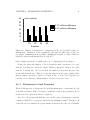
Empirical Evaluation . . . . . . . . . . . . . . . . . . . . . . . . . . .
90
4.6.1
Simulation Setup . . . . . . . . . . . . . . . . . . . . . . . . .
90
4.6.2
Construction . . . . . . . . . . . . . . . . . . . . . . . . . . .
90
4.6.3
Robustness to Link Dynamics . . . . . . . . . . . . . . . . . .
91
4.6.4
Packet Loss and Routing Quality . . . . . . . . . . . . . . . .
92
4.6.5
Improving Routing Diversity . . . . . . . . . . . . . . . . . . .
94
Summary and Remarks . . . . . . . . . . . . . . . . . . . . . . . . . .
95
5 Conclusion
97
Bibliography
99
ix
List of Figures
1.1
Interference model. . . . . . . . . . . . . . . . . . . . . . . . . . . . .
5
1.2
Network skeleton and network sketch. . . . . . . . . . . . . . . . . . .
9
1.3
Examples of information potentials. . . . . . . . . . . . . . . . . . . .
10
2.1
In a “good” communication graph, transmission power should depend
on node density. . . . . . . . . . . . . . . . . . . . . . . . . . . . . . .
15
2.2
Local neighborhood size. . . . . . . . . . . . . . . . . . . . . . . . . .
23
2.3
For the proof of Lemma 11. . . . . . . . . . . . . . . . . . . . . . . .
36
3.1
Network sketching example. . . . . . . . . . . . . . . . . . . . . . . .
41
3.2
Network sketching as infrastructure. . . . . . . . . . . . . . . . . . . .
42
3.3
Boundary cycle orientation ambiguity. . . . . . . . . . . . . . . . . .
44
3.4
Combinatorial Delaunay graph is not always planar. . . . . . . . . . .
49
3.5
For the proof of Lemma 16. . . . . . . . . . . . . . . . . . . . . . . .
52
3.6
For the proof of Theorem 2. . . . . . . . . . . . . . . . . . . . . . . .
52
3.7
For the proof of Lemma 17. . . . . . . . . . . . . . . . . . . . . . . .
54
3.8
For the proof of Lemma 18. . . . . . . . . . . . . . . . . . . . . . . .
56
3.9
For the proof of Lemma 21. . . . . . . . . . . . . . . . . . . . . . . .
61
3.10 Face collapse in barycentric embedding. . . . . . . . . . . . . . . . . .
65
3.11 Irregular shape of the sensor field has no effect. . . . . . . . . . . . .
67
3.12 Evolution of the seed cycle in embedding heuristic. . . . . . . . . . .
68
3.13 The effect of varying landmark density. . . . . . . . . . . . . . . . . .
69
3.14 Performance on a sparse network. . . . . . . . . . . . . . . . . . . . .
70
3.15 The sketching pipeline. . . . . . . . . . . . . . . . . . . . . . . . . . .
71
x
4.1
A simple reactive (diffusion-based) method for information discovery.
77
4.2
Examples of solutions to the discrete Laplace equation. . . . . . . . .
82
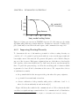
4.3
Trivial potential function in a large part of the network as a result of
poor connectivity. . . . . . . . . . . . . . . . . . . . . . . . . . . . . .
4.4
87
Greedy paths on information potentials avoid the 0-boundary, which
balancing length and robustness.
. . . . . . . . . . . . . . . . . . . .
88
4.5
Robustness to link addition and deletion. . . . . . . . . . . . . . . . .
89
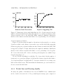
4.6
Initial construction of information potential. . . . . . . . . . . . . . .
91
4.7
Cost of maintaining information potential after a single link failure. .
92
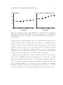
4.8
Cost of maintaining information potential after a single link failure as
a function of network size. . . . . . . . . . . . . . . . . . . . . . . . .
93
Query success rate in the lossy model. . . . . . . . . . . . . . . . . .
94
4.10 Traffic balancing by randomizing query paths. . . . . . . . . . . . . .
95
4.9
xi
Chapter 1
Introduction
The infrastructure of a wireless sensor network is a set of per-node data structures
that sensor nodes need to build upon deployment, in order to be able to communicate reliably and perform higher-level tasks related to user’s application. This includes
discovery of other nodes within communication range, selecting a set of communication partners, assigning radio frequencies, synchronizing local clocks, setting up basic
routing mechanisms etc. These problems are some of the most fundamental issues in
sensor networks.
In this thesis we address several problems in this class: communication graph establishment and channel assignment (Chapter 2), autonomous discovery of geographic
and topological features of a given deployment (Chapter 3), point-to-point routing
(Chapter 3), and data-centered routing (Chapter 4). In Chapter 5 we summarize our
results and propose directions for further research.
1.1
1.1.1
Preliminaries
Notation
We use standard terminology and notation related to sets and graphs. In this section
we only point out a few conventions that might otherwise confuse the reader.
For a set A, we denote its size by |A|. A singleton set A = {a} may also be
1
2
CHAPTER 1. INTRODUCTION
denoted by a.
We denote graph edges using ordered pairs. For directed graphs (a, b) denoted
an edge from a to b. For undirected graphs, the ordering is irrelevant, i.e. (a, b) and
(b, a) denote the same edge. It will always be clear from the context if the graph in
question is directed or undirected.
In a directed graph, incoming (resp. outgoing) neighbors of a vertex a, denoted
by N in (a) (resp. N out (a)) are all nodes b such that (b, a) is an edge (resp. (a, b) is
an edge). The neighbors of a vertex a, denoted by N (a), are incoming and outgoing
neighbors of a. In an undirected graph, the neighbors of a vertex a, denoted by N (a),
are all nodes b such that (a, b) is an edge. We denote the incoming and outgoing
degrees of node u in an undirected graph by degin (u) and degout (u), respectively. The
total degree of node u in an undirected or directed graph is denoted by deg(u). If
needed, we specify the relevant graph in the subscript; for example, for graph G we
write NGout (u) and degout
G (u).
An (incoming, outgoing) neighborhood of a set A of vertices is the union of corresponding (incoming, outgoing) neighborhoods of all elements of A. Neighborhoods
are also called 1-hop neighborhoods. For an integer h ≥ 2, an h-hop neighborhood is
a 1-hop neighborhood of a (h − 1)-hop neighborhood.
Graph vertices will often correspond to points in some Euclidean space, and we
will denote a vertex and the corresponding point using the same symbol. If a and b
are two such vertices/points, then |ab| is the Euclidean distance between the points,
whereas d(a, b) is the distance (number of edges in the shortest path) in the graph.
For edge e = (a, b), we define |e| = |ab|. If A and B are sets of vertices/points, then
|AB| =
min
(a,b)∈A×B
|ab| ,
d(A, B) =
min
(a,b)∈A×B
d(a, b) .
We will use standard concepts from theory of metric spaces, usually applied to
the Euclidean spaces with | · | metric and graphs with d(·, ·) metric, as defined above.
The ball of radius r centered at x is denoted by B(x, r). A set is an r-cover if the
union of balls centered at elements of A is the whole space. A set is an r-packing if
no two elements of A are closer than r.
3
CHAPTER 1. INTRODUCTION
A graph is planar if it can be drawn in the plane so that no two edges intersect
except at vertices. Such a drawing we will refer to as planar embedding.
A simple path (cycle) is a path (cycle) that has no self-intersections. We use this
term for both graph paths (cycles), where self-intersection means passing through a
graph vertex more than once, as well as for geometric paths (cycles) in the plane,
where self-intersection means passing through a point in the plane more than once.
1.1.2
Sensor Nodes
We assume that each node u has a unique identifier (ID), which we assume to be an
integer. Throughout, we will use u to denote both the node and its unique integer ID.
In particlar, if u, v are nodes, then u can be included in a message to be transmitted,
or u and v can be compared as in u < v. Immediately upon deployment, each node’s
ID is known only to that node. We assume that the sensor nodes are very small, and
that they lie in a common plane (e.g., flat ground). Hence we model them as point
in two-dimensional space. Unless noted otherwise, point and node are synonyms, and
the total number of nodes in the network in n. The phrase with high probability
(w.h.p.) means with probability at least 1 −
1
,
nc
where c is a constant that can be
made arbitrarily large.
1.1.3
Ad-Hoc Deployment
Infrastructure establishment problem is most interesting when sensor nodes are deployed in an ad-hoc fashion, i.e., when node placement is not fully controlled by the
network designer. For example, monitoring environmental conditions in an inaccessible part of a rainforest may call for an ad-hoc deployment by scattering sensor nodes
from an airplane.
It should be noted that not all sensor network deployments are ad-hoc. For example, sensors that monitor lighting conditions in “smart buildings” are manually deployed. Their software can already contain prior knowledge in the form of a “typical”
topology which the network can “tweak” when necessary, to handle local fluctuations
in radio connectivity.
CHAPTER 1. INTRODUCTION
1.1.4
4
Communication Model
If v is within radio range of u, we say that v is a (communication) neighbor of u.
Communication graph contains information about pairs of nodes that can communicate. Its vertices are nodes, and there is a directed edge from u to v if and only if v
is a communication neighbor of u. An undirected edge represents two directed edges
with the same endpoints and opposite orientations.
We assume disk graph communication model, defined as follows. Radio range of
node u is a disk centered at u, which we call the transmission disk (range) of u. The
transmission radius of u is the radius of u’s transmission disk, and it is proportional
to u’s transmission power.
Under this assumption, the communication graph is a disk graph (DG): v is a
communication neighbor of u if and only if v is contained in u’s transmission disk.
In general, the graph is directed. If all transmission powers (equivalently, radii) are
equal, it is undirected, and is called a unit-disk graph (UDG). We use UDG(r) to
denote the communication graph corresponding to common transmission radius r.
1.1.5
Interference Model
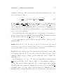
Due to interference, a message sent by node u may not be received by its intended
recipient v if another node w, physically close enough to v so that it shares a part of
v’s medium (Figure 1.1), transmits a message at the same time as u, using the same
carrier frequency as u. Then, u’s message to v collides with w’s message. This is
often called hidden terminal problem, with v being the hidden terminal. As a special
case, w can in fact be v, i.e., v’s reception can be prevented by v’s own transmission.
We assume that collisions can be detected — a receiving node can distinguish
between situations when the number of signals it receives is zero (corresponding to
no reception at all) and more than one (corresponding to a collision). Of course, the
message is actually received only if there is no collision, i.e., if exactly one signal is
received.
Collisions can be handled proactively and reactively. Reactive approach resolves
collisions after they happen using a handshake mechanism. Typically, conflicting
5
CHAPTER 1. INTRODUCTION
w
u
v
Figure 1.1: Transmission from u cannot be received by v because it collides with
transmission from w.
nodes wait for a certain, often “random”, amount of time before retransmitting.
These backoff intervals are designed to ensure that a successful transmission eventually occurs. Clearly, if transmission powers are such that any two nodes are within
each other’s range, it may take Ω(n) time for a handshake to succeed. Proactive
approach avoids collisions altogether, and is based on standard techniques of timeand frequency-division multiple access, i.e., assigning time slots or carrier frequencies,
respectively, to nodes so that any two nodes whose are assigned different values if
their transmissions would otherwise collide.
In this thesis we adopt proactive method for handling collisions. Specifically, the
algorithm in Chapter 2 computes a schedule of transmissions, i.e., it assigns time
slots to nodes in such a way that if each node transmits in its assigned time slot, no
collisions occur. The length of the schedule is the number of time slots used by all
nodes. The algorithm can be trivially adapted to work with frequency-based instead
of time-based multiplexing. This will become clear after we present the details in
Chapter 2.
1.1.6
Pseudocode
We assume that all variables are global (visible to all subroutines executing on a given
node) and there is no parameter passing. We use subscripts to refer to values of a
variable at a specific node. A variable with no subscript is assumed to be stored at
the node executing the code. For example, in Algorithm 4 (Section 2.4.2), node u
is executing the code (as specified in the caption), so TRIAL and TRIALu refer to
CHAPTER 1. INTRODUCTION
6
the value of variable TRIAL at node u, while TRIALv refers to the value of variable
TRIAL at node v received by u. We use the keyword wait to denote waiting for the
next tick of the local clock. Other keywords should be self-explanatory.
1.2
Thesis Outline
Sensor networks are embedded in physical space, and knowing the geometry of that
space ought to be useful in computing good infrastructure. In this thesis we study
how much is achievable without geometric information. To this end, all our algorithms
are designed to work with deployments which are fully ad-hoc, i.e., where no prior
knowledge about deployment geometry, such as geographic locations or distances, is
available (Section 1.1.3).
In each chapter we present an algorithm for establishing one kind of sensor network infrastructure. Algorithms are presented in increasing order of abstraction, from
very low-level establishment of individual communication links from scratch (Chapter 2), to establishment of the information brokerage paths that conform to the global
geometric shape of the network (Chapter 4), with each algorithm building on the preceding one.
Chapters 2, 3, and 4 are based on [23], [24], and [48], respectively.
1.2.1
Computing Communication Graph
In ad-hoc deployments, no connectivity information is available at programming time,
and the network has to be formed by nodes themselves upon deployment. As defined
in Section 1.1.4, communication graph encodes pairs of nodes within radio range, for
a given assignment of communication powers to nodes. The topic of Chapter 2 is
the problem of computing a set of transmission powers, the induced communication
graph, and a collision-avoiding time schedule of transmissions (Section 1.1.5).
Using higher transmission power results in a better connected communication
graph, but also creates more interference, which increases the smallest achievable
schedule length. The goal is to maximize connectivity of the communication graph,
CHAPTER 1. INTRODUCTION
7
and minimize the length of the schedule. Additional goal to minimize the number of
communication rounds required to compute the graph and the schedule.
There are many algorithms that compute communication graphs ignoring interference, and many that prevent or resolve collisions in known communication graphs.
However, to the best of our knowledge, no algorithm solves both problems simultaneously, and this is the core of our contribution.
The algorithm in Chapter 2 computes a communication graph that is well connected in the sense that it contains an energy-optimal path between any two nodes,
and a collision-avoiding time schedule whose length is bounded by the spatial gradient of node density1 . The running time is logarithmic in n and linear in the gradient
of node density. The algorithm is distributed and local, i.e., only requires communication between nodes that are direct neighbors with respect to the current choice of
communication powers. It assumes disk graph communication model (Section 1.1.4)
and clock synchronization.
If each node can localize itself, the algorithm can be adapted to compute communication graphs defined using node locations [65, 25, 70, 45], with properties like
short paths, small node degrees, planarity, support for efficient routing etc, which are
useful, even crucial, for some applications [6, 33].
The output of this algorithm can be used by higher-level applications (such as the
infrastructure establishment algorithms presented in Chapters 3 and 4) can use it as
a “clean” graph abstraction of the underlying sensor network whose edges represent
links that support reliable, atomic communication.
1.2.2
Sketching Location-Unaware Networks
Chapter 2 shows that freshly deployed nodes, without any initial knowledge about
each other, can form a well connected, interference-free network. Now assume that
nodes “cover” (form a dense sampling of) some connected region in the plane. Such
node distributions are common in applications, because it is often important that each
point of some area of interest be monitored by a sensor node. Chapter 3 shows that it
1
The notion of energy-optimal path and spatial gradient will be made formal in Chapter 2.
CHAPTER 1. INTRODUCTION
8
is possible to infer the topology of the region “covered” by sensors using only network
connectivity. Roughly speaking, inferring topology means drawing the communication
graph in the plane in such a way that the region covered by the nodes in the drawing is
topologically equivalent to (i.e., can be continuously “morphed” into) the true region.
Although clearly less valuable than true geometric information, topology is still
useful. For example, suppose that the area covered by the network is not simply
connected, i.e., it has holes. This often happens in real deployments because sensors
cannot be deployed everywhere in the region of interest (e.g. walls, obstacles, forest
fires, lakes, hillsides etc.). Then, topology contains information like the number of
holes, the identities of nodes along the hole boundaries, etc. The data discovery
algorithm in Chapter 4 benefits from this information. Also, just like exact geometric
layout can be used to facilitate routing [6, 33], a topologically equivalent layout can
serve the same purpose (more about the routing application below).
Existing algorithms for computing network topology2 from its communication
graph [63, 22, 36, 68] are limited to detecting the boundary of the region, rather than
computing its realization in the plane.
The algorithm presented in Chapter 3 is motivated by fact that relating an abstract
graph to the topology of its underlying space is easier if the graph is a well connected
planar graph, because for such graphs there is essentially only one planar embedding,
which can also be efficiently computed.
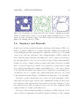
Assuming disk graph communication model (Section 1.1.4) and node density high
enough relative to the size of geometric features of the sensor field (narrow “passages”
and high-curvature boundaries), the algorithm computes a provably planar and well
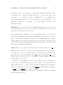
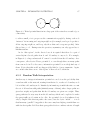
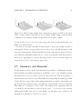
connected subgraph of the input communication graph (Figure 1.2 left), and its planar
embedding called network sketch (Figure 1.2 right). Network sketch captures network
topology in the sense that the union of its “small” faces (those adjacent to a number
of nodes below some absolute constant) has the correct topology. In other words,
“large” faces correspond to areas empty of sensors — finite faces to holes and the
infinite face to the “outside world”.
In general, “virtual” coordinates of nodes given by network sketch differ from real
2
If not specified otherwise, network topology means topology of the region covered by the network.
CHAPTER 1. INTRODUCTION
9
Figure 1.2: Planar “skeleton” (left) extracted from the communication graph, and its
planar embedding, the network sketch (right).
ones, i.e., the sketch is not guaranteed to be geometrically close to the original network
layout. However, nothing prevents their usage in protocols that are normally designed
to work with real geographic locations. For example, geographic routing, a simple local
routing paradigm originally defined for localized networks [6, 33, 40, 41, 39] provably
works in location-unaware networks when implemented using network sketches.
1.2.3
Data Discovery Using Information Potentials
In Chapter 4 we propose a way to use existing connectivity and topology infrastructure, discussed in Chapters 2 and 3 respectively, for information discovery and
brokerage among mobile producers and consumers of data.
A node acts as information producer if it detects an event or a data source in
its proximity3 . Data is always associated with a type, and it is assumed that the
type can be easily inferred from the data by the node itself. If a node detects a user
interested in certain data type, it becomes an information consumer for that type.
The goal of data discovery infrastructure is to connect the information consumers in a
communication-efficient way to one or more producers of their desired data type. Data
discovery is essential for sensor networks deployed in “human spaces”, i.e. occupying
the same physical space as its users (in contrast to, for instance, a community of
scientists collecting information from a remote observation site).
3
The mechanism of detecting events from raw data is not essential for the algorithm.
CHAPTER 1. INTRODUCTION
10
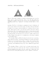
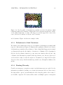
Figure 1.3: Information potential corresponding to a single data source (left), and to
a set of two data sources (right). The latter is obtained using composability.
We consider an application scenario in which the set of producers and consumers
is highly dynamic, for example due to mobility of participants, “burstiness” of data
sources and/or user interests. Combined with usual dynamics of network connectivity,
this creates significant robustness challenges.
In Chapter 4 we present a novel data discovery protocol that exploits existing
infrastructure given by the communication graph (Chapter 2) and network sketch
(Chapter 3). We propose to “diffuse” information away from source nodes holding
desired data, so as to establish information potentials that allow network queries
to navigate towards and reach these sources through local greedy decisions, following
information gradients. See Figure 1.3 (left) for an example of an information potential
of a single source.
We compute these information potentials by solving for a discrete version of the
Laplace equation with Dirichlet boundary conditions. We use boundary conditions
to encode knowledge of the physical network boundary. As a result, information
potential “knows” the shape of the network, and “ranks” nodes based on the their
distance to both data source and the boundary. Roughly speaking, a node has high
potential if it has a “corridor” to the data source which is “short” but also comparably
“wide”.
The solutions to the Laplace equation are classical harmonic functions, which have
a rich algebraic structure and many useful properties.
• Information potentials have no local maxima other than the source nodes, guaranteeing success of greedy routing using information gradient. This is what
CHAPTER 1. INTRODUCTION
11
enables the basic data discovery function.
• Information potentials can be computed using a simple iterative algorithm,
called Jacobi method [4, 3], that can be executed in a distributed manner, with
nodes exchanging information only with their network neighbors.
• The Jacobi method can be re-invoked to repair the information field when links
fail. Also, because of the aforementioned prefernce for “wide” paths, alternative
paths may be available even without any repair. We present empirical results
showing that these two properties (robust paths and quick repair of broken
paths) lead to high query success rate even with realistically modeled unrelaible
links.
• A (pointwise) linear combination of information potentials is a potential for the
union of sources (Figure 1.3 right). If there are many simultaneous queries for
the same of sources (e.g. sources of a given fixed data type), each query can
use a different linear combination of “basis” potentials, yielding an inexpensive
way to spread the communication load associated with these queries.
Chapter 2
Computing the Communication
Graph
In this chapter we present an algorithm for assigning transmission powers to sensor
nodes and computing the induced communication graph. The computation is done
in-network, without any pre-existing infrastructure, and with node deployment initially unknown to the algorithm. In particular, medium access problem has not been
solved, i.e., nearby nodes cannot transmit at the same time. In these conditions,
there is a tradeoff between connectivity and running time. Better connectivity of the
communication graph requires higher transmission power. This in turn causes more
interference, which takes more time to resolve. Our algorithm produces a graph which
is well connected (contains a power-optimal path between any two nodes), and yet
exhibits low interference so that it can be computed in a small number of time steps
(communication rounds).
In addition to assigning transmission powers and computing the associated communication graph, the algorithm also produces a efficient schedule of node transmissions that can be used (by higher-level infrastructure and application-level algorithms) for interference-free communication on the resulting communication graph.
The above mentioned fact that the output communication graph exhibits low interference also implies that the length of its transmission schedule (the number of time
slots in which every node can transmit once without any collisions) is small.
12
CHAPTER 2. COMPUTING THE COMMUNICATION GRAPH
13
The most important feature of the algorithm is that it computes both communication graph and a transmission schedule “from scratch” — other algorithms typically
assume one to compute the other. In particular, it explicitly deals with interference
while computing the graph. The algorithm is fully distributed and localized, i.e., only
nearby nodes communicate and store information about each other. We show that
the algorithm is especially fast when the spatial variations of node density are slow,
which is often the case in ad-hoc deployments.
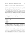
The rest of this chapter is organized as follows. In Section 2.1 we introduce the
problem of computing communication graphs, and discuss importance of location
information and variable transmission power in achieving good connectivity with
low interference. We give a detailed statement of our results in Section 2.2, and a
comparison with with existing approaches in Section 2.3. Section 2.4 describes our
algorithm in detail and analyzes its performance. In Section 2.5 we present a class
of deployments for which our algorithm performs particularly well. We conclude in
Section 2.6 with some remarks.
2.1
Communication Graph as Infrastructure
In Section 1.1.4 we defined the communication graph as an undirected graph which
encodes possible transmitter–receiver pairs, and introduced the disk graph radio propagation model in which communication graph depends on node locations and transmission powers. In ad-hoc deployments, node locations are unknown at programming
time, so it is impossible to precompute and assign transmission powers that nodes
should use in order to form a “good” communication graph. Instead, the graph has
to be computed by the nodes themselves, once they have been deployed. The main
topic of this chapter is an algorithm for computing a well connected communication
graph for a set of nodes initially unknown to the algorithm, and with no pre-existing
infrastructure of any kind.
Since the computation takes place in-network, it has to take interference into
account. In other words, we want an algorithm that maintains some kind of collision handling mechanism (Section 1.1.5) while it computes the graph. By contrast,
CHAPTER 2. COMPUTING THE COMMUNICATION GRAPH
14
most existing algorithms for computing communication graphs ignore interference
and assume atomic, reliable communication. The algorithm presented in this chapter
handles collisions using time-based multiplexing. Specifically, it maintains a schedule
of transmissions — assignment of time slots to nodes such that if each node transmits
in its assigned time slot using its assigned transmission power, no collisions occur. In
addition to maintaining a collision-avoiding transmission schedule during computation, our algorithm also produces a schedule which is valid for the output graph that
it computes.
Communication graph, equipped with a collision resolution mechanism such as
transmission schedule, is the most basic form of network infrastructure. It provides a
“clean” graph abstraction of the network, in which communication over a chosen link
is atomic operation, guaranteed to succeed. High-level applications, including most
existing algorithms for establishing other types of infrastructure (network localization,
routing, information brokerage), depend upon the ability of nodes within each other’s
radio range to exchange information reliably. Using this abstraction, they can be
implemented without worrying about low-level radio propagation effects and radio
interference.
2.1.1
Geometric Communication Graphs
Even though different application have somewhat different notions of a “good” communication graph, one common requirement is good connectivity. It is also desirable
that the topology be computed quickly after deployment, reducing the overall network
setup time. Finally, the communication graph should be accompanied by an efficient
(short) schedule of transmissions, an assignment of time slots to nodes, such that
all collisions are avoided if each node transmits with assigned transmission power in
assigned time slot.
However, the three goals conflict. Better connectivity requires higher transmission
power, which in turn induces more interference. As a result, it takes more time slots
to schedule a round of transmissions (one from each node) so as to avoid collisions.
Also, computing the schedule may take more time and communication.
CHAPTER 2. COMPUTING THE COMMUNICATION GRAPH
15
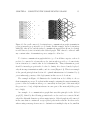
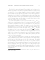
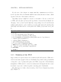
Figure 2.1: In a well-connected, low-interference communication graph, transmission
power is inversely proportional to node density. In this example, any node interferes
with O(1) other nodes, and the induced communication graph (not shown, for clarity)
is well-connected, since it includes the Gabriel graph. This cannot be achieved with
any constant value of transmission power, assigned to all nodes.
To obtain a communication graph which is “good” in all three aspects, each node
needs to be connected to a few nearby nodes, just enough to provide good connectivity,
but not interfere too much other nodes’ transmissions. Thus, transmission power
should be inversely proportional to local node density: if nodes are densely deployed,
only short-range transmissions suffice, and vice versa (Figure 2.1). This is an example
of the general principle from Section 4.1: optimal infrastructure is determined by (a
priori unknown) geometry of the deployment, in this case node locations.
The example in Figure 2.1 illustrates the benefit from nodes’ ability to choose
their transmission powers. Note that in this example, assigning the same transmission
power to all nodes results in either poor connectivity in some part of the network (if
the power is too low) or high interference in some part of the network (if the power
is too high).
An example of a communication graph that uses this principle is the Gabriel
graph [25], defined by the following geometric rule: nodes u and v are connected if and
only if the disk with diameter uv is has empty interior. Gabriel graph is well connected
in the sense that it contains all energy-optimal paths in the network. In other words,
when routing a message from source to destination via multiple relay nodes, smallest
CHAPTER 2. COMPUTING THE COMMUNICATION GRAPH
16
possible energy expenditure can be achieved by using only transmissions represented
by Gabriel edges1 . In particular, the Gabriel graph is connected, i.e., there is a path
between any two nodes.
Apart from good connectivity, Gabriel graph is also planar (Section 1.1.1), which
can be exploited in location-based routing [6, 33]. Planarity also implies sparsity —
the average degree of the Gabriel graph, like any planar graph, is less than 6, which
bounds the amount of local storage that a node needs (on average) to store information
associated with its neighbors (such as input/output buffers).
2.2
Contribution
In this chapter we present an algorithm for computing
• an assignment of transmission powers to nodes,
• a communication graph induced by that power assignment
• a time schedule of transmissions (one transmission per node) which guarantees
absence of collisions, i.e., interference-free transmissions.
The main advantage of our algorithm is the fact that it computes all three components
“from scratch”, i.e., without assuming pre-existing infrastructure.
The output communication graph is well-connected, in the sense that it contains
the Gabriel graph, w.h.p. (the algorithm is randomized). The length of the transmission schedule is O(∆), and the running time is O(∆ log
rmax
rmin
log2 n), where rmin (resp.
rmax ) are minimum (resp. maximum) distance between any two nodes, and ∆ is the
maximum number of nodes “near” any Gabriel edge — more precisely, within c times
the length of the edge, for a constant c that will be determined later. Intuitively, ∆
captures the worst-case number of nodes that can interfere with computation of any
edge that we insist on including in the final communication graph, i.e., any Gabriel
edge. Therefore, it is natural that performance degrades as ∆ increases.
1
This holds under the assumption that the transmission power (in the unit disk radio model,
Section 1.1.4) grows at least quadratically with transmission radius, which is often true in practice.
CHAPTER 2. COMPUTING THE COMMUNICATION GRAPH
17
How big is ∆ for various deployments? Even though it can be as large as n for
arbitrary deployments, we show that for deployments in which node density is locally
near-uniform (i.e., does not change abruptly, as a function of spatial coordinates),
then ∆ is small. We argue that such deployments are often found in applications.
In particular, if node density2 is an α-Lipschitz function with α small enough, then
∆ = O(1). The main reason why only local uniformity is required lies in the definition
of ∆: the relevant distance scale (the length of a nearby Gabriel edge) is locally
defined, and “adapts” to the local node density.
To execute the algorithm, nodes need to know the values of ∆, rmin and rmax .
In the absence of any information about node locations, true values can be replaced
by estimates (overestimates for ∆ and rmax , underestimate for rmin ), with performance guarantees changing accordingly. For example, rmin can be lower-bounded
using physical size of a node, and rmax can be upper-bounded using diameter of the
sensor field. In Section 2.6 we discuss other ways to select rmin and rmax . Note that
the estimate need not be very accurate, since the dependence on
rmax
rmin
is logarithmic.
To upper bound ∆, one needs to estimate the worst-case spatial variation of node
density. Also, n always works as an upper bound on ∆. Whatever the estimated
values are, they need to be equal at all nodes. Finally, the algoritrhm requires that
nodes’ local clocks be synchronized.
Some of the previous results hold more generally. One can make sure that the
output communication graph contains any fixed graph (instead of the Gabriel graph),
provided that ∆ is defined with respect to the edges of that graph. The running
time and scheduling bounds in terms of ∆, rmin and rmax do not change. The fact
that ∆ is small for locally near-uniform deployments does not hold in general, but it
holds for graphs that connect only “nearby” pairs of nodes, like the relative neighborhood graph [65], Yao graph [70], localized Delaunay graphs [45] etc. For clarity,
all proofs in this chapter deal with the Gabriel graph; adapting them to other cases
is straightforward.
2
Later in the chapter we will define a scalar function, defined on the plane, which serves as a
measure of node density.
CHAPTER 2. COMPUTING THE COMMUNICATION GRAPH
18
We assumed in the beginning that node locations are not known, and that is the
reason that our final communication graph is not equal to the Gabriel graph, but
only a supergraph thereof. If, however, each node knows its own location (e.g., by
having a built-in positioning device like GPS), but not locations of any other node, we
argue (referring to [23] for full proofs) that our algorithm can be extended to compute
exact Gabriel graph, with only a slight increase in running time. We also conjecture
that the algorithm be modified to compute some other geometrically defined “local”
graphs (relative neighborhood graph, localized Delaunay graph and Yao graph).
2.3
Related Work
Efficient distributed computation of communication graphs (often called topology control) and interference-avoiding transmission schedules have attracted a lot of attention
in the past. In this section we review existing algorithms for similar problems.
In [9] and [2], the authors introduce a quantity that can be computed for a given
communication graph in the plane, and serves as a measure of interference. Then
they propose centralized algorithms for computing communication graphs with low
interference. In [10], a connected dominating set of small size, constructed in a
centralized fashion, is used to obtain a communication graph.
A number of distributed algorithms [46, 47, 67] compute communication graphs
with desirable properties (like sparsity, bounded degree, planarity etc.) using an existing communication graph that does not have those properties, but whose links are
interference-free. So the goal is not to establish network “from scratch”, but rather assuming that the interference problem has already been solved. The only way to apply
these algorithms to our problem is to compute this “supporting” network beforehand
and make it interference-free by appropriate transmission scheduling. However, this
is very similar to the problem that we are trying to solve.
A number of algorithms compute a schedule of transmissions, but for a known
communication graph given as input [57, 60, 61]. Typically, the problem becomes
a variant of graph coloring which is then solved in a centralized fashion, exactly or
approximately, depending on the class of allowed input graphs.
CHAPTER 2. COMPUTING THE COMMUNICATION GRAPH
19
In a more realistic model [55, 37, 52] (which is also closest to the one we consider),
only power assignment and radio propagation model are known, while the induced
communication graph has to be computed in the presence of interference before transmissions on it can be scheduled. Our work further relaxes this model by introducing
flexibility in choosing transmission powers. However, unlike [37, 52], we assume that
collisions can be detected. A variant of the distributed algorithms in [55] will be used
in our approach as a subroutine.
Recent work of Moscibroda et al. [54, 53, 50] consider arbitrary, known communication graphs and algorithms for computing good power assignments and schedules.
Their algorithms are centralized, but guarantee good schedules for arbitrary networks
and use a more realistic model of interference, where signal and noise powers are
modeled explicitly, including their polynomial decay with distance, and a reception
is successful if signal-to-noise ratio at the receiver exceeds a given threshold.
2.4
The Algorithm
In this section we present the main result of this chapter. We start with the high-level
description of the main idea.
For the rest of this chapter, we will use lu to denote the longest Gabriel edge
adjacent to node u. Let (u, v) be the longest Gabriel edge adjacent to u. Obviously,
one way for u to learn all its Gabriel neighbors is to learn about all nodes in B(u, l u ).
This can be accomplished by having each node send a message with radius lu , announcing their presence. Then, ideally, u receives messages exactly from nodes in
B(u, lu ). In reality, however, there are two problems. First, some of the messages
from u’s neighbors to u may collide, so u may not learn about some of its Gabriel
neighbors. Second, single Gabriel edges are not known in advance, neither is lu .
We solve the first problem by scheduling messages, so that collisions are avoided.
Recall that the algorithm takes as input parameter ∆, the maximum number of nodes
that are “near” any Gabriel edge, where by “near” we mean at a distance at most
a constant times the length of the edge. The key observation is that the number of
nodes that can cause collisions is at most ∆, because all of them have to be “near”
CHAPTER 2. COMPUTING THE COMMUNICATION GRAPH
20
Gabriel edge (u, v). This implies, as it turns out, that transmissions can be scheduled
in about ∆ time slots, even in the distributed way. We solve the second problem
by “sweeping” the entire range of possible values of transmission radius r, trying to
“guess” the value of lu .
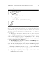
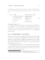
More formally, provided with parameters rmin and rmax , each node locally executes
e rounds (iterations of the main loop, lines 2 –
Algorithm 1, which consists of dlog rrmax
min
7). Each round corresponds to a value of transmission radius r, which increases by a
Algorithm 1 Main
1: r ← rmin
2: while r < rmax do
3:
Exploration
4:
TempSchedule
5:
Edges
6:
r ← 2r
7: end while
8: FinalSchedule
factor of 2 between rounds.
The communication graph is initially empty. According to the above description,
the goal of the round with radius r is to discover all nodes within distance r from
some subset of nodes for which r is a “good” communication radius. This motivates
the following definition.
Definition 1 A node is said to be active in a round with radius r if it is adjacent to
a Gabriel edge of length at least 2r . A node which is not active is called inactive.
Intuitively, r is a “good” communication radius for all nodes that are active in round
with radius r. Obviously, all nodes are active before the first round, and inactive
after the last round.
In each round, u first announces its presence to all other nodes within distance
r and listens to announcements from other nodes (line 3). Clearly, all received announcements are from nodes in B(u, r), but announcements of some nodes in B(u, r)
may not get through to u due to interference. To test if all neighbors have been
discovered, nodes compute a temporary transmission schedule (line 4) to be used only
CHAPTER 2. COMPUTING THE COMMUNICATION GRAPH
21
during the current round. The idea is to have all nodes announce themselves again,
but this time following an interference-avoiding schedule. Line 5 performs this test
and, if successful, creates edges from u to all discovered neighbors of u. If the test
fails, u creates no edges in the current round. Note that we expect the test to succeed
whenever r if u is an active node, and to fail when r is too large compared to the
length of any Gabriel edges adjacent to u.
After the end of the last round, u accepts the result of the last round in which its
test succeeded, i.e., sets the communication radius and the set of neighbors from that
round. It remains to schedule transmissions over the resulting communication graph,
which is done in line 8 using a procedure similar to that for computing temporary
schedules.
It is tempting to think that the test is unnecessary, because it cannot hurt to
create new edges to all discovered neighbors. However, this would actually create very
long edges (significantly longer than any adjacent Gabriel edge). High interference
caused by those edges would make it more difficult to compute the final transmission
schedule.
In the next four sections we explain each of the four subroutines in more detail.
Since the Exploration, TempSchedule and Edges subroutines operate with a fixed
communication radius r during a single round, in the next three sections (2.4.1,
2.4.2 and 2.4.3), we assume for brevity that all graph-related terms (hops, neighbors,
neighborhoods etc.) refer to UDG(r) unless noted otherwise. Also, we will sometimes
use ri to denote the radius corresponding to round i. Rounds are counted starting
from 1, so clearly ri = rmin 2i−1 .
2.4.1
Neighborhood Exploration
The goal of the Exploration subroutine is to ensure that active nodes (and some
near neighbors of active nodes, which will be needed later) successfully learn their
1-hop neighbors in UDG(r).
The pseudocode is shown as Algorithm 2. Each node stores its neighbors discovered so far in variable M , which is the main output of Exploration. The subroutine
CHAPTER 2. COMPUTING THE COMMUNICATION GRAPH
22
consists of I = O(log n) rounds (line 2), each of which is 2∆ time steps long (line 4).
In each round a node chooses a random integer t between 1 and 2∆ (line 3) and
transmits its ID at time step t of current round within radius r (line 6). In remaining rounds, it listens to other nodes’ announcements (line 9) and adds them to M
(line 10).
Algorithm 2 Exploration
1: M ← ∅
2: for i = 1, 2, . . . , I do
3:
t ← uniformly at random from {1, 2, . . . , 2∆}
4:
for j = 1, 2, . . . , 2∆ do
5:
if j = t then
6:
transmit u within radius r
7:
else
8:
if no collision then
9:
receive v
10:
M ← M ∪ {v}
11:
end if
12:
end if
13:
wait
14:
end for
15: end for
We pointed out in the introduction that the parameter ∆ passed to the algorithm
should be an upper bound on the number of nodes “near” any Gabriel edge, where
“near” is understood relative to the length of the edge. This is formalized in the
following definition.
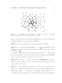
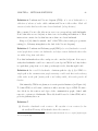
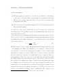
Definition 2 k-local neighborhood size of u, denoted by ∆k (u), is the number of
nodes contained in a disk B(u, klu ). k-local neighborhood size of the network is
∆k = maxu∈V ∆k (u).
See Figure 2.2 for an illustration. Observe that ∆k is a monotonically non-decreasing
function of k.
The following lemma shows that, as we argued informally, local neighborhood
sizes bound the number of nodes that can interfere with communication to and from
CHAPTER 2. COMPUTING THE COMMUNICATION GRAPH
23
u
Figure 2.2: Local neighborhood sizes ∆1 (u) = 5, ∆2 (u) = 12, ∆3 (u) = 20. Only
Gabriel edges adjacent to u and its neighbors are shown.
active nodes, when all nodes use the same transmission power. More precisely, they
bound the neighborhood of any active node in UDG(r).
Lemma 1 An active node has at most ∆2h h-hop neighbors in UDG(r).
Proof. Let u be active in round with radius r, so lu ≥ 2r . h-hop neighbors of u in
UDG(r) are contained in B(u, hr) ⊆ B(u, 2hlu ), so there are at most ∆2h of them,
by Definition 1.
The main result of this section is that parameter ∆ should be no smaller than
2(h+1)-local neighborhood size of the network in order to guarantee successful neighborhood discovery in the h-hop neighborhood of active nodes.
Lemma 2 If ∆ ≥ ∆2(h+1) , then upon termination of Exploration at all nodes,
all h-hop neighbors of all active nodes contain their (1-hop) neighborhoods in their
respective M variables w.h.p.
Proof. Let v be an arbitrary h-hop neighbor of u, and let w be an arbitrary 1-hop
neighbor of v. An announcement from w can collide only with an announcement from
another 1-hop neighbor x of v. All such x are clearly (h + 1)-hop neighbors of u, so
by Lemma 1, there are at most ∆2(h+1) of them, which is at most ∆, by assumption.
CHAPTER 2. COMPUTING THE COMMUNICATION GRAPH
24
On the other hand, w chooses its time slot from a pool of size 2∆. It follows that v
learns about w with probability at least
1
2
each time w transmits, and therefore w.h.p.
in I = O(log n) transmissions, for large enough constant in I. The claim follows by
union bound over all choices for u and v.
Note that nodes themselves do not know at this point if their neighborhood discovery succeeded or not. In order to test this, a temporary schedule of transmissions
needs to be computed, which is the subject of the next section.
2.4.2
Temporary Schedule
The goal of the TempSchedule subroutine (line 4 in Algorithm 1) in the round
with radius r, is to compute a temporary schedule which allows for collision-free communication, during the current round, between active nodes and their neighbors in
UDG(r). Recall that we are only concerned with neighborhoods of active nodes, because all Gabriel edges adjacent to inactive nodes are short, and have been computed
in previous rounds.
The following lemma introduces sufficient conditions for interference-free communication that our algorithm will aim to satisfy.
Lemma 3 Communication between active nodes and their neighbors is interferencefree if the following pairs of nodes never transmit simultaneously:
(i) an active node and another node within 2 hops from it,
(ii) two nodes in the 1-hop neighborhood of some active node.
Proof. Let u be an active node and let v be its neighbor. Since condition (i) holds,
v can receive transmissions from u without interference. Since condition (ii) holds, u
can receive transmission from v without interference.
Our algorithm is a slight variation of the one proposed in [55]. Next, we sketch
the latter and briefly discuss the required changes.
CHAPTER 2. COMPUTING THE COMMUNICATION GRAPH
25
The Distance-Two-Coloring Algorithm of Parthasarathy and Gandhi
Parathasarathy and Gandhi [55] presented an algorithm for distance-two-coloring,
i.e., assigning colors (integers) to nodes so that no two nodes within two hops of each
other are assigned the same color. Their algorithm assumes that each node knows its
1-hop neighbors and a bound on the number of 2-hop neighbors.
Refer to Algorithm 3. Each node maintains a list L of potential colors it can
choose from. Initially the list has 2C colors (line 1), and the number decreases over
time. In the end, variable t will contain the chosen color for each node. The algorithm
proceeds in rounds. In a typical round, some yet-uncolored nodes choose a color from
their list, and if this color has not been chosen by any 2-hop neighbors, these color
assignments become permanent, and all 2-hop neighbors remove the respective colors
from their lists. The algorithm terminates after I rounds. One round consists of 4
phases: Trial, TrialReport, Success, and SuccessReport.
Algorithm 3 DistanceTwoColoring
1: L ← {1, 2, . . . , 2C}
2: for i = 1, 2, . . . , I do
3:
Trial
4:
TrialReport
5:
Success
6:
SuccessReport
7: end for
The Trial phase (Algorithm 4) consists of 2C time slots. An uncolored node u
chooses a random color t from its list, and transmit a TRIAL message (u, t) in the time
slot corresponding to the chosen color. In other time slots it listens for other nodes’
TRIAL messages (line 9), which it concatenates into a TRIAL-REPORT message
(line 10).
The TrialReport phase (Algorithm 5) consists of B blocks of 2C time slots each.
In every block, a node chooses a random time slot among the 2C slots available in
a block, and sends its TRIAL-REPORT message. In all other slots, it listens to
other nodes’ TRIAL-REPORT messages, which it uses to determine if the color it
had chosen in the Trial phase is safe. The color is safe if TRIAL-REPORT messages
CHAPTER 2. COMPUTING THE COMMUNICATION GRAPH
26
Algorithm 4 Trial
1: if t = 0 then
2:
t ← uniformly random from L
3:
for j = 1, 2, . . . , 2C do
4:
if j = t then
5:
TRIAL ← (u, t)
6:
transmit TRIAL within radius r
7:
else
8:
if no collision then
9:
receive TRIALv
10:
TRIAL-REPORT ← (TRIAL-REPORT, TRIALv )
11:
end if
12:
end if
13:
wait
14:
end for
15: end if
have been received from all neighbors (line 20), each contains u (line 9), and none
contains the same color chosen by another node (line 12). Otherwise, the color is reset
(lines 10, 13 and 21). Note that knowledge of 1-hop neighborhood M is required to
perform this test.
The Success phase (Algorithm 6) consists of 2C time slots. Any colored node
u sends a SUCCESS message (u, t) in the time slot corresponding to its color tu ,
and in other time slots listens for other nodes’ SUCCESS messages (line 7), which it
concatenates into a SUCCESS-REPORT message (line 8). Note that newly colored
nodes will not participate in future Trial phases.
The SuccessReport phase (Algorithm 7) is similar to the TrialReport phase.
Nodes send their SUCCESS-REPORT messages in random time slots over B rounds,
and in other time slots they listen for other nodes’ SUCCESS-REPORT messages
(line 8), removing from their lists all colors contained in received messages (line 10).
Parthasarathy and Gandhi prove that if I = O(log n), B = O(log n), the following
three facts hold for any node u w.h.p. (we refer to [55] for details).
(a) A 2-hop neighbor of u (which is possibly u itself) can remain uncolored only if
it has more than C 2-hop neighbors.
CHAPTER 2. COMPUTING THE COMMUNICATION GRAPH
27
Algorithm 5 TrialReport
1: for i = 1, 2, . . . , B do
2:
c ← uniformly at random from {1, 2, . . . , 2C}
3:
for j = 1, 2, . . . , 2C do
4:
if j = c then
5:
transmit TRIAL-REPORT within radius r
6:
else
7:
if no collision then
8:
receive TRIAL-REPORTv
9:
if TRIAL-REPORTv does not contain TRIALu then
10:
t←0
11:
end if
12:
if TRIAL-REPORTv contains TRIALw s.t. w 6= u and tw = tu then
13:
t←0
14:
end if
15:
end if
16:
end if
17:
wait
18:
end for
19: end for
20: if TRIAL-REPORTv not received for some v ∈ M then
21:
t←0
22: end if
Algorithm 6 Success
1: for j = 1, 2, . . . , 2C do
2:
if j = t then
3:
SUCCESS ← (u, t)
4:
transmit SUCCESS within radius r
5:
else
6:
if no collision then
7:
receive SUCCESSv
8:
SUCCESS-REPORT ← (SUCCESS-REPORT, SUCCESSv )
9:
end if
10:
end if
11:
wait
12: end for
CHAPTER 2. COMPUTING THE COMMUNICATION GRAPH
28
Algorithm 7 SuccessReport
1: for i = 1, 2, . . . , B do
2:
c ← uniformly at random from{1, 2, . . . , 2C}
3:
for j = 1, 2, . . . , 2C do
4:
if j = c then
5:
transmit SUCCESS-REPORT within radius r
6:
else
7:
if no collision then
8:
receive SUCCESS-REPORTv
9:
if SUCCESS-REPORTv contains SUCCESSw = (w, tw ) then
10:
L ← L \ {tw }
11:
end if
12:
end if
13:
end if
14:
wait
15:
end for
16: end for
(b) Let v be a 2-hop neighbor of u. Assuming both u and v are colored, their
colors can be the same only if all their common neighbors x (including u and v
themselves, if u and v are adjacent) have more than C 2-hop neighbors.
(c) Let v and w be 1-hop neighbors of u (notice that v or w may be the same as u).
Assuming that, v and w are both colored, their colors can be the same only if
all their common neighbors x (including v and w, if v and w are adjacent) have
more than C 2-hop neighbors; in particular, only if u has more than C 2-hop
neighbors.
Note that in all three cases, the “bad event” occurs if some node has more than C
2-hop neighbors. So, Parthasarathy and Gandhi conclude that if C is set to be the
maximum size of any 2-hop neighborhood3 , then the result is a valid distance-twocoloring with probability at least 1 − n−χ for arbitrary χ > 0 (the constant factors
for C, I, B depend on χ). Clearly, the overall running time is O(C log 2 n).
3
In fact they set C to be the maximum size of any 1-hop neighborhood. Since for UDGs this is
within a constant factor from the maximum size of any 2-hop neighborhood, only the constants for
I, C, B change.
CHAPTER 2. COMPUTING THE COMMUNICATION GRAPH
29
What are the implications of this result in our case? Obviously, we would like to
use the distance-two-coloring algorithm to schedule transmissions in UDG(r), with
colors naturally corresponding to time slots in the schedule. Applying the algorithm
of [55] directly yields a schedule of length C computable in time O(C log 2 n). There
are two problems with this approach.
• Some nodes may not know their neighbors, and therefore may not be able to
perform the check in the Success phase.
• Maximum number of 2-hop neighbors can be as large as n, so setting C as in [55]
leads to a poor schedule length and computation time.
Fortunately, we do not really need a distance-two-coloring on UDG(r), but merely one
that satisfies the conditions of Lemma 3. It is not hard to see that the conditions of
Lemma 3 are satisfied if the properties (a), (b), (c) above hold for all active nodes u,
as opposed to all nodes u — (a) and (b) imply (i), while (a) and (c) imply (ii). After
this relaxation, the obstacles to applying the algorithm of [55] become less severe
• Only 2-hop neighbors of u need to execute the Success phase correctly, so only
they need to know their 1-hop neighborhoods.
• Also, when we look more carefully into (a), (b), (c), we see that “bad events”
occur only if some 2-hop neighbor of u has more than C 2-hop neighbors, which
happens only if u has more than C 4-hop neighbors.
By Lemma 2 with h = 2, 2-hop neighbors of active nodes know their 1-hop neighbors
if ∆ ≥ ∆6 . By Lemma 1, any active node can have at most ∆8 4-hop neighbors, so
“bad events” do not happen if C ≥ ∆8 .
Our subroutine TempSchedule is actually the DistanceTwoColoring algo-
rithm of [55] with C = ∆. Preceding discussion then proves the main result of this
section.
Lemma 4 If ∆ ≥ ∆8 , then upon termination of TempSchedule at all nodes u,
communication between all active nodes and their 1-hop neighbors is interference-free
w.h.p.
CHAPTER 2. COMPUTING THE COMMUNICATION GRAPH
2.4.3
30
Finding Edges
The Edges procedure (line 5 in Algorithm 1) adds or removes edges from the final
communication graph. The problem is to decide whether the radius r of the current
round is greater or smaller than lu , the length of the longest Gabriel edge adjacent to
u. Ideally, we would like to create edges if and only if r ≤ lu . The idea is to use the
number of “nearby” nodes as a proxy — create edges in round with radius r if and
only if the number of nodes in a larger concentric ball B(u, cr), for some constant c,
does not exceed the maximum number of nodes that can ever be found in that ball,
expressed in terms of an appropriate local neighborhood size (Definition 2).
Implementation is shown as Algorithm 8. The main output variables are the set
of neighbors N and the communication radius ρ, which are also outputs of the main
algorithm, once the final round has completed. The remaining piece of the output,
the transmission schedule, is computed by FinalSchedule, as explained in the next
section.
Lines 1 – 20 compare the number of “nearby” nodes of u in the current round to
a threshold ∆. To compare the number of neighbors to the threshold ∆, each nodes
announces its presence once more by sending a single message, this time not in a
random time slot (as in Exploration), but according to the temporary schedule. In
other time slots, each node simply collects other nodes’ announcements. The result
of the comparison is stored in the Boolean variable ok. It is equal to true if and
only if the node has collected at most ∆ announcements and has not experienced any
collisions.
The comparison is “fuzzy” in the sense that different outcomes use different definitions of “nearby”. ok=true implies that the number of neighbors (nodes in B(u, r))
is at most ∆, while ok=false implies that the number of nodes in B(u, 4r) is greater
than ∆. This is formalized in Lemma 5 and Lemma 6, respectively.
Lemma 5 If ok=true, then |N | ≤ ∆ and N is exactly the set of u’s neighbors.
Proof. If |N | > ∆, then ok=false by line 19. Hence |N | ≤ ∆. Obviously, all
nodes in N are neighbors of u. If there was a neighbor v of u which is not in N ,
CHAPTER 2. COMPUTING THE COMMUNICATION GRAPH
Algorithm 8 Edges
1: N 0 ← ∅
2: ok ← true
3: for i = 1, 2, . . . , 2∆ do
4:
if i = tu then
5:
transmit u with radius r
6:
else
7:
if no collision then
8:
receive v
9:
N 0 ← N 0 ∪ {v}
10:
end if
11:
else
12:
if collision then
13:
ok ← false
14:
end if
15:
end if
16:
wait
17: end for
18: if ok and |N 0 | > ∆ then
19:
ok ← false
20: end if
21: if ok then
22:
Label edges in N 0 \ N by i
23:
N ← N0
24:
ρ←r
25: else
26:
N ← N \ edges of N added for the first time in rounds i − 4 and later
r
27:
ρ ← 32
28: end if
31
CHAPTER 2. COMPUTING THE COMMUNICATION GRAPH
32
its transmission (line 5) must have collided, so ok=false (line 13), a contradiction.
Hence N is exactly the set of u’s neighbors.
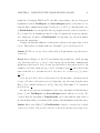
Lemma 6 If r is the radius of the current round, and B(u, 4r) has at most ∆ nodes,
then ok=true.
Proof. Clearly, u has at most ∆ 4-hop neighbors. The same argument as in the
proof of Lemma 4 proves that communication between u and its neighbors in the
current round is interference-free, so transmissions in line 5 so not collide. It follows
that N is equal to the set of u’s neighbors. Since B(u, r) ⊆ B(u, 4r), u has at most
∆ neighbors, so |N | ≤ ∆.
We need to satisfy two properties
(i) All Gabriel edges are included.
(ii) All edges (u, v) such that B(u, 9|uv|) contains more than ∆ nodes are excluded.
This will be useful for computing the final transmission schedule in Section 2.4.4.
Property (ii) can be satisfied by creating edges to all neighbors whenever ok=true
(line 23), and removing all edges created in the preceding 3 rounds whenever ok=false
(line 26).
Lemma 7 For any edge (u, v) of the final communication graph B(u, 16|uv|) contains
at most ∆ nodes.
Proof. Let i be the last round in which (u, v) was added. Assume without loss
of generality that round i + 4 exists (otherwise consider the last round j ∈ {i +
1, i + 2, i + 3} that exists, and observe that B(u, 16|uv|) contains the same nodes as
B(u, 2j−i |uv|)). Since |uv| ≤ ri =
ri+4
,
16
we have B(u, 16|uv|) ⊆ B(u, ri+4 ). Clearly,
(u, v) is not removed in round i+4, so ok=true in that round. By Lemma 5, B(u, ri+4 )
has at most ∆ nodes.
So far the value of ∆ was arbitrary, i.e., it only used the fact that ∆ is the same
as in Exploration and TempSchedule. However, to make sure that (i) is satisfied,
∆ has to be large enough.
33
CHAPTER 2. COMPUTING THE COMMUNICATION GRAPH
Lemma 8 If ∆ ≥ ∆8 , then any Gabriel edge (u, v) is added to the final communica-
tion graph in the (unique) round i in which
ri
2
< |uv| ≤ ri .
Proof. Clearly, u is active in round i. By Lemma 1, B(u, 4r) contains at most ∆8
nodes. By Lemma 6, ok=true in this round. By Lemma 5, v ∈ N , so (u, v) is added
in line 23.
Lemma 9 If ∆ ≥ ∆128 , no Gabriel edge is ever removed from the final communication graph.
Proof. Suppose that node u removes edge (u, v) in round i. Obviously, ok=false
in round i, so by Lemma 6, B(u, 4ri ) has more than ∆ nodes, which is more than
∆128 nodes. Let j be the first round in which (u, v) was added. Obviously, j ∈
{i − 4, i − 3, i − 2, i − 1}, so ri ≤ 16rj , and B(u, 4ri ) ⊆ B(u, 64rj ). It follows that
B(u, 64rj ) contains more than ∆128 nodes, so we have 64rj ≥ 128lu , i.e., lu ≤
|uv| >
rj
,
2
rj
.
2
If
then |uv| > lu , so (u, v) is not a Gabriel edge. Otherwise, let k be the
unique round in which
rk
2
< |uv| ≤ rk . Since |uv| ≤
rj
,
2
we have k < j. By choice of
j, (u, v) was not added in round k, so by Lemma 8 it is not a Gabriel edge.
Lemma 10 If ∆ ≥ ∆128 , then the final communication graph contains the Gabriel
graph.
Proof. Follows from Lemma 8 and Lemma 9.
2.4.4
Final Schedule
The goal of the FinalSchedule subroutine (line 8 in Algorithm 1) is to compute a
final schedule of transmissions which allows for collision-free communication on the
final communication graph computed by the main loop of Algorithm 1. Of course,
the rest of this section is conditioned on the fact that at the start of the procedure
final communication graph has been correctly computed, i.e., each node knows its
outgoing neighbors. From the previous discussion we know that this happens w.h.p.
with correct parameter choices.
CHAPTER 2. COMPUTING THE COMMUNICATION GRAPH
34
The main difference with respect to temporary transmission schedules, computed
by TempSchedule, is that the latter correspond to UDGs, while in the former case
nodes use different transmission powers. This means, for instance, that the nodes
that can interfere with communication between a given node u and its neighbors are
no longer contained in B(u, r), where r is u’s transmission radius.
The algorithm of [55] cannot be directly applied, because it is designed for UDGs.
Specifically, it may happen that nodes u and v propose the same time slot in the
Trial phase, and their messages collide, but all nodes that experience the collision
cannot report it to u and v because its communication radii are too small.
Fortunately, there is a simple modification that gets around this problem without
affecting the asymptotic performance.
(i) In the Trial (resp. Success) phase a node transmits within its final radius. In
addition to its ID and a proposed (resp. assigned) time slot, it also transmits
the value of its final radius.
(ii) In the TrialReport (resp. SuccessReport) phase, a node transmits within
the radius equal to the maximum radius received in the preceding Trial (resp.
Success) phase. Note that this radius is always at least as large as the final
communication radius.
(iii) When fixing a time slot (after receiving a TRIAL-REPORT message) and removing time slots from the list (after receiving a SUCCESS-REPORT message),
a given node only takes into account messages received from its outgoing neighbors.
(i) ensures that the collisions generated are exactly those that would occur in the
output communication graph. (ii) and (iii) ensure that the scheduling is correct, but
(ii) may hurt the running time — increasing the radii for the reporting purpose may
create additional collisions among the report messages. However, we show that the
same value of parameter ∆ used in the previous stages of the algorithm still suffices.
In Section 2.4.2 we observed that correctness of Parthasarathy and Gandhi distancetwo-coloring algorithm [55] follows from upper bound of ∆ on the size of any 2-hop
CHAPTER 2. COMPUTING THE COMMUNICATION GRAPH
35
neighborhoods in input UDG. Let G be the DG corresponding to the set of increased
transmission radii in TrialReport and SuccessReport phases. Obviously, G contains the final communication graph. For the proof of [55] to go through in the case
of FinalSchedule, it is enough that all 2-hop neighbors in the undirected version of
G be bounded by ∆. Intuitively, this is because G captures the worst-case interference during the execution of FinalSchedule, and ignoring edge directions further
increases the interference.
It turns out that this sufficient condition indeed holds for the same value of ∆ as
before. This is where we finally make use of Lemma 7, proved in Section 2.4.3.
Lemma 11 The size of any 2-hop neighborhood in G ignoring the edge directions is
at most ∆.
Proof. Refer to Figure 2.3. Let N be an arbitrary 2-hop neighborhood in G, ignoring
edge directions, and let e = (u, v) be the longest edge in the final communication
graph whose head is in N . Let e0 be any edge in G whose both vertices are in N . By
definition of G, there exists an edge e00 in G, of length at least
|e0 |
,
2
whose head is the
same as the tail of e0 , and therefore in N . By choice of e, we have |e00 | ≤ |e|, hence
|e0 |
2
≤ |e|.
Now, any node in N can be reached from u by following first e, and then at most
4 edges of G whose both vertices are in N (ignoring edge directions along the way).
Hence, N is contained in B(u, |e| + 4|e0 |) ⊆ B(u, 9|e|). By Lemma 7, N contains at
most ∆ nodes.
In other words, increased transmission radii create only limited additional interference, so the TrialReport and SuccessReport phases still succeed w.h.p. We
conclude that the algorithm of TempSchedule can be run with the same value of
∆, and the final values of t variables will contain a valid transmission schedule w.h.p.
Lemma 12 In time O(∆ log2 n), FinalSchedule computes a transmission schedule
(stored in t variables) that prevents collisions in the final communication graph w.h.p.
CHAPTER 2. COMPUTING THE COMMUNICATION GRAPH
e
N
e00
e0
36
u
v
Figure 2.3: For the proof of Lemma 11 – bounding the size of a 2-hop neighborhood
in the modified DG.
2.5
Lipschitz Deployments
Theorem 1 yields better results (faster algorithm and shorter transmission schedule)
if parameter ∆ is smaller. Of course, the value of ∆ is lower bounded by “intrinsic
interference” measured by ∆128 . In this section we introduce a class of deployments,
called Lipschitz deployments, for which this “intrinsic interference” is low, in the sense
that ∆128 does not depend on the number of nodes n.
Lipschitz deployments are those in which a certain measure of node density (defined below), cannot change too abruptly between two nearby points in the area of
interest. Such slowly varying node density is often found in practice. For instance,
consider a sensor network whose goal is to monitor physical quantities (such as temperature, humidity, exposure to light etc.) in a nature preserve. Suppose that there
is a set of points H that describes interesting “hot spots” to be monitored more accurately. The goal is to deploy more sensors close to the “hot spots”, and fewer sensors
further away.
For example, “hot spots” can be small animals that should be tracked by the
network. To minimize the work spent in adapting the sensor placement to animal migrations, it is reasonable to have a gradually increasing sensor density as the distance
to an object (in its current position) decreases.
Formally, assume that there is a scalar “interest function” f , defined on the plane,
which is small in regions of high interest and vice versa. An example is f (x) = |xH|,
37
CHAPTER 2. COMPUTING THE COMMUNICATION GRAPH
the distance to the closest “hot spot”, for any metric d defined on the plane. Then,
a well-deployed set of sensors V should satisfy |xV | ≤ εf (x) for any point x and
some fixed ε > 0. On the other hand, to minimize the cost of equipment, only
the necessary number should be used; in terms of the “interest function” f , the
appropriate condition is: for any point x, |V ∩ B(x, εf (x))| is bounded by some
universal constant β.
Definition 3 A set of nodes V is an (α, β)-Lipschitz deployment, for if there exists
an α-Lipschitz function ϕ, defined on the plane, such that for any point x, the disk
B(x, ϕ(x)) contains between 1 and β nodes.
The deployment in the example above is (ε, β)-Lipschitz (distance to a fixed set of
points is a 1-Lipschitz function). Observe that Definition 3 also allows for “oversampling” of the domain of interest, as long as the oversampling happens in a slowlyvarying manner. It also allows coverage holes (large areas with no sensors), as long
as sensor density increases gradually with distance from the hole. Now we prove the
main property of Lipschitz deployments.
Lemma 13 For an (α, β)-Lipschitz deployment, ∆k = O((k + 1)2 β) for k <
1
4α
− 1.
Proof. Consider a fixed node u, and let (u, v) be the longest Gabriel edge adjacent to
u, so that |uv| = lu . Let x be the midpoint of (u, v). Because (u, v) is a Gabriel edge,
any ball centered at x with radius less than
lu
2
is empty, which implies
lu
2
≤ ϕ(x).
Clearly, ∆k ≤ |V ∩ B(x, (k + 1)lu )|, so it suffices to bound the number of nodes in
B(x, R), where R = (k + 1)lu .
Using the above inequalities, we get R ≤ 2(k + 1)ϕ(x). As ϕ is α-Lipschitz, we
have for any y ∈ B(x, R) that ϕ(y) ≥ ϕ(x) − αR ≥ ϕ(x)(1 − 2(k + 1)α), that is, any
disk of radius at most r = ϕ(x)(1 − 2(k + 1)α) centered within B(x, R) contains less
k+1
)2 ) such disks. By assumption,
than β nodes. B(x, R) can be covered by O(( 1−2(k+1)α
α<
1
,
4(k+1)
k+1
so O(( 1−2(k+1)α
)2 β) = O((k + 1)2 β)
From this we directly derive a class of node deployments for which our algorithm
performs particularly well.
CHAPTER 2. COMPUTING THE COMMUNICATION GRAPH
Corollary 1 For an (α, β)-Lipschitz deployment with α <
1
916
38
and β = O(1), Algo-
log2 n) time steps, and produces a schedule of length O(1).
rithm 1 takes O(log rrmax
min
Of course, theoretical analysis in this section is very pessimistic and we expect the
algorithm to perform very well for many practical node distributions.
2.6
Summary and Remarks
We summarize the statements of Lemmas 2, 4, 10, and 12 in our main theorem.
Theorem 1 Let lu be the length of the longest Gabriel edge adjacent to node u, and
let ∆ be the maximum, over all u, number of nodes in B(u, 128lu ). Algorithm 1
runs in O(∆ log rrmax
log2 n) time and w.h.p. computes a communication graph that
min
contains the Gabriel graph, and a schedule of transmissions of length 2∆ which ensures
interference-free communication in this graph.
0
rmin can be replaced by any value rmin
such that the number of nodes contained in
0
any disk of radius 128rmin
is bounded by ∆. The lower bound on ∆ can be decreased
from ∆128 to ∆k for k < 128, by discretizing the range of transmission radii more
finely, i.e., using a constant smaller than 2 as multiplication factor for the geometric
progression. Finally, one may have an upper bound on the length of any Gabriel edge
(for instance if the deployment is known to be very dense). In that case rmax can be
set to that value.
If exact locations are available, which we do not assume in this thesis, the algorithm can be modified to compute exact Gabriel and an associated transmission
schedule. The main difference is in procedure Edges (Section 2.4.3). While in
Edges, edges can be safely created to all discovered neighbors (set N in Algorithm 8)
without any extra communication, in the analogous procedure GabrielEdges additional communication is required to check the Gabriel property for each edge. Notice
that the maximum number of Gabriel edge that can be created by one node in one
round is ∆. It turns out that, with help of the temporary transmission schedule of
length 2∆, computed previously by TempSchedule (Section 2.4.2), all checks can
be done in O(∆3/2 ) time steps per round. As a result, entire algorithm runs in time
CHAPTER 2. COMPUTING THE COMMUNICATION GRAPH
39
min
O(∆3/2 log rrmax
log2 n). Also, the lower bound on parameter ∆ is weaker, ∆ ≥ ∆8 .
We refer to [23] for details.
It can be ensured that the output communication graph contains any desired set
of edges (e.g., Gabriel graph, relative neighborhood graph, Yao graph etc.), provided
that the algorithm is given a value of parameter ∆ which is suitable for that set of
edges, i.e., a valid upper bound on the 128-local neighborhood size ∆128 . We expect
∆128 to be small for “local” topologies (in which each node is connected only to
nearby nodes) and Lipschitz deployments (in which node density has bounded spatial
variations). In particular, we have shown that ∆128 for the set of Gabriel edges.
Chapter 3
Network Sketching
In main topic of this chapter is an algorithm that computes a rough geometric layout
of the network using only connectivity information (the communication graph). The
restriction to connectivity information is motivated by the fact that real-world sensor
nodes more often than not lack the ability to determine their own location. Localization devices are usually not built-in because in the interest of minimizing cost and
maximizing network lifetime by saving energy. For example, GPS devices are too
energy-expensive for most applications. Furthermore, their performance can be poor
indoors.
The algorithm presented in this chapter first finds a planar subgraph of the communication graph, a skeleton of the network (Figure 3.1 left), and then computes its
embedding in the plane (Figure 3.1 right). The idea is to exploit the fact that embedding of a planar graph is combinatorially unique, provided sufficient connectivity,
so the embedding preserves the skeleton layout up to “stretching”. The embedding
yields virtual coordinates of the nodes in the skeleton, which can be used instead of
the real coordinates in several applications outlined below.
The algorithm should be viewed as a generic method for relaxing localization
requirements. It does not provide an accurate localization as is, but it reduces the
amount of geometric information required to obtain one, by decoupling the problem
of localizing the skeleton from the problem of localizing all other nodes with respect
to the skeleton.
40
CHAPTER 3. NETWORK SKETCHING
41
Figure 3.1: Using no location information, our algorithm computes a provably planar
subgraph of the communication graph (network skeleton) and its plane embedding.
The numbers denote corresponding nodes in the embedding and the original node
layout, which is unknown to our algorithm. Although the two layouts are different in
terms of absolute node coordinates, the network sketch is topologically correct (large
faces and correspond to holes).
3.1
Network Sketch as Infrastructure
Network sketch contains information about topology of the area covered by sensor
network (which we will also call sensor field). Informally, this means that the network
sketch is an image of the original sensor field under a “morphing” transformation
which does not change the connectivity; in particular, it does not “tear” the area into
multiple components, or form new “holes” by creating new adjacencies of the sensor
field with itself. For example, in Figure 3.1, the network sketch can be obtained from
the true sensor field by a vertical flip followed by a 90◦ clockwise rotation. Topology
information can be exploited in several application scenarios, such as hole detection
and routing.
Holes are connected areas that are empty of nodes. For example, if nodes are
deployed from the air, they can roll down a hillside, fall into a lake and short-circuit
etc., resulting in creation of holes. In some applications hole detection is the goal
in its own right, because holes represent events of interest. For example, in forest
CHAPTER 3. NETWORK SKETCHING
42
Figure 3.2: Applications of network sketching: environmental monitoring (left), highlevel route planning (center) and geographic routing (right).
fire tracking, holes correspond to areas where sensors have been destroyed after being deployment from the air (Figure 3.2 left). In network health monitoring, holes
correspond to areas where nodes ran out of energy due to increased activity for an
extended period. Being topologically equivalent to the original sensor, a network
sketch preserves identity of nodes on hole boundaries, and can be used as a building
block in these applications.
Topology awareness is crucial ingredient for guaranteeing message delivery in
location-based (geographic) routing algorithms. In the simple greedy forwarding method,
the rule is to always forward the packet to neighbor which is closest to the destination, in terms of Euclidean distance. The method is scalable, as its routing tables
are simplified due to geographic side-information — a node only needs to know the
locations of its neighbors and the destination in order to decide how to forward a
packet. However, greedy forwarding may not be possible if no neighbor is closer to
the destination than the node currently holding the packet, i.e., if the packet is at a
local minimum of the distance function. Due to the properties of Euclidean distance
function, such local minima only appear at hole boundaries.
One way to combat this problem, proposed in [19], is to compute a sparse subnetwork of “highways” (Figure 3.2 center) on which even non-geographic routing is not
too expensive, while “local” routing between the “highway network” and individual
nodes always takes place over short distances, and is therefore less likely to suffer from
the local minimum problem. Network sketch, or some suitable subgraph thereof, can
CHAPTER 3. NETWORK SKETCHING
43
be used for this purpose.
Another approach is to circumnavigate holes that cause local minima of the distance function (Figure 3.2 right). This is typically done by precomputing an embedded
planar subnetwork whose face cycles roughly follow the hole boundaries, and then,
when needed, routing around the face cycles using the “right hand rule” [6, 33]. However, computing the planar subnetwork is not trivial, and most existing approaches
rely on node locations for both planarization and embedding. Network sketching
makes it possible to apply this strategy even in location-unaware networks, because
it produces a embedded planar subgraph using only connectivity information.
Topology information can be exploited in other applications, such as data aggregation and information brokerage, to optimize the way in which information is moved
across the network. This will be the topic of Chapter 4. If additional geometric
measurements are available (e.g. locations of a few “anchor” nodes), they can used
to make the sketch more similar to the true network layout. This improved sketch
can then be used in applications that depend on true node locations, rather than just
topology of the sensor field.
3.2
Related Work
There have been a number of papers that aim to extract structural information about
the network by analyzing its communication graph. In this section we classify them
into those that detect boundaries (either as sets of nodes that lie near boundaries or
proper boundary cycles), and those that also provide a geometric embedding. Note
that obtaining an embedding from the set of boundary cycles is not trivial, because
of the cycle orientation ambiguity (Figure 3.3). Our algorithm can also be seen as a
way of resolving this ambiguity by examining how boundary cycles are connected to
each other through the interior.
First we discuss methods that only detect holes, but do not compute an embedding. Algorithm of Fekete et al. [22] assumes that node placement is governed by a
Poisson process of constant (but unknown) density over the sensor field. It distinguishes boundary nodes from interior nodes using the difference in their degrees. The
44
CHAPTER 3. NETWORK SKETCHING
c
c
f
d
a
f
e
e
b
a
d
b
Figure 3.3: If the relative orientation of boundary cycles in the plane is not correct, the
interior cannot be embedded in the plane. Left: a correct embedding. Right: after
changing the orientation of the face cycle cdf , the cycle acf d surrounds e in any
embedding (even the very “complicated” one shown), and thus cannot be a face
cycle.
algorithm of Kroöller et al. [36] makes no assumptions about node distribution. It
detects groups of interior nodes and the graph cycles that provably surround them.
It classifies a node as interior only if its neighborhood contains an elaborate “flower
graph”, which is why it seems to work only under restrictive theoretical conditions
(dense interior). The cycles are small at first, and in the second stage they merge until
they become boundary cycles. Even though the results are proved to be correct in any
unit-disk embedding of the network, it is not clear how to actually compute an embedding. Merging cycles requires a lot of communication, so the message complexity
of the algorithm is O(n3 ).
The algorithm of Funke and Klein [63] analyzes how the level-sets of certain hopdistance functions break into components upon hitting hole boundaries. The method
identifies a set of nodes that forms a provably good sample of hole boundaries. However, it does not connect the nodes into boundary cycles. It also requires good network
connectivity, even in simulations (average degree of the communication graph around
20).
The algorithm of Wang et al. [68] is based on detecting critical points of the
distance from a fixed source in the sensor field. The key observation is that such
points have multiple shortest paths to the source, which can be combined into cycles
that enclose holes. It subsequent stages these cycles are “tightened” around holes.
CHAPTER 3. NETWORK SKETCHING
45
Our planar skeleton (Section 3.4.1) is similar to witness complex of de Silva and
Carlsson [16]. If X is a metric space, Y is its subset, and point x ∈ X has exactly
k + 1 nearest neighbors in Y , then the set of nearest neighbors in called a k-simplex
witnessed by x. The witness complex is the set of all simplices defined in this way. The
vertices and edges of our planar graph are similar to 0- and 1-simplices, respectively,
of the witness complex under the hop-distance. We add extra conditions to guarantee
planarity and make efficient embedding possible.
Recent work of de Silva and Ghrist [17] addresses similar problems of topology
discovery in location-free networks using algebraic topology – homology of certain
simplicial complexes derived from the communication graph. Because the approach is
not based on planar graphs, but on more complicated higher-dimensional complexes,
it does not seem to allow for an efficient embedding procedure.
Now we turn to methods that compute an embedding. The problem that has
attracted the most attention is that of achieving low distortion, i.e. the worst-case
Euclidean distance (in the embedding) between two adjacent nodes in the network. It
is possible to embed a network in the plane with distortion polylogarithmic in n [51,
56]. Low distortion directly translates into low path stretch, so it is important for
routing. However, it does not imply geometric or topological accuracy of the layout.
Embedding algorithms in [51, 56] solve convex optimization problems distributedly,
so they are quite communication-expensive.
Multidimensional scaling (MDS) [14] is a classic embedding technique which computes a point set whose distance matrix is the best least-squares approximation to a
given matrix. When applied to sensor network localization [62, 13], distance matrices
can be obtained from time of arrival measurements, received signal strength measurements, or simply hop-distances. Error components are typically weighted according
to the reliability of the corresponding distance measurement, and various models
are used to estimate the latter. Unfortunately, MDS does not guarantee topological
accuracy.
Rao et al. [58] use barycentric embedding [66] to compute its two-dimensional
embedding in a distributed way, but the result is not guaranteed to preserve geometry
or topology of the sensor field. In fact, we use the same embedding technique — not
CHAPTER 3. NETWORK SKETCHING
46
on the whole network, but only on the skeleton. In our case topology is preserved,
due to the properties of the skeleton.
3.3
Contribution
In this chapter we present an algorithm for sketching the layout of a wireless network
represented only by its communication graph. Under the unit-disk communication
model, and sufficiently high node density in the interior, Our algorithm extracts
a skeleton of the network, a provably planar graph whose long face cycles follow
the boundaries of holes in the (unknown) true layout. The algorithm outputs a
sketch of the network, which is simply a planar embedding of the skeleton. Under
the same assumptions, we prove that this embedding is topologically correct, in the
sense that all boundary cycles are correctly oriented (cf. Figure 3.3). The actual
locations of the nodes in the skeleton need not be correct, but they can be improved
if additional inter-node distances or node locations are available. Sufficient node
density is required to guarantee sufficient connectivity of the skeleton, which in turn
relates to its “embeddability”. Even though theoretical density requirements are
unrealistic, our experiments show that the skeleton is reasonably well connected even
when they are not satisfied.
3.4
The Algorithm
Our network skeleton is actually a subnetwork called combinatorial Delaunay map
(CDM), a discrete analog of Delaunay triangulation in computational geometry ([15],
Chapter 9). The motivation comes from the fact that Delaunay triangulation is always
planar, and the goal is to preserve this property in discrete setting. In short, we do
this by viewing nodes as discrete samples of the underlying area, replacing Euclidean
by hop-distance in the network, and adding some extra “robustness” conditions on
Delaunay edges, to account for discretization effects. Once we have computed the
CDM, we compute its planar embedding using the barycentric algorithm [66].
CHAPTER 3. NETWORK SKETCHING
47
For the rest of the chapter we assume unit-disk communication model (Section 1.1.4), where all nodes transmit with the same radius, known in advance, which
depends on the size of the features of the area.
Algorithm 9 shows a high-level overview of our method. For two cycles C1 , C2
of CDM, d(C1 , C2 ) (line 9) denotes the hop-distance between their landmark sets.
“Merging” of face cycles C1 and C2 (line 10) corresponding to faces F1 and F2 means
adding together the face cycles of all faces on some path between F1 and F2 in the
dual graph, such that any face on the path is also within tl hops from both C1 and
C2 .
Algorithm 9 Main
1: k ← 34
2: ts ← face size threshold (see Theorem 4)
3: td ← face distance threshold (see Theorem 4)
4: select landmarks as a maximal k-packing (with respect to hop-distance)
5: compute CVD by Definition 4
6: compute CDM by Definition 8
7: embed CDM using any algorithm
8: C ← face cycles of length more than ts
9: while ∃C1 , C2 ∈ C such that d(C1 , C2 ) ≤ td do
10:
merge C1 and C2 , updating C appropriately
11: end while
12: return C
3.4.1
Definition of the CDM
Suppose that we are given a subset of nodes which we will call landmarks. CDM can be
viewed as an abstract graph on the set of landmarks. In geometric analogy, landmarks
correspond to a set of points in the plane, and CDM corresponds to their Delaunay
triangulation. CDM can also be viewed as a subnetwork of the input network, because
its abstract edges can be realized as paths connecting pairs of landmarks.
The first step is to define a discrete analog of the Voronoi diagram in geometry
([15], Chapter 7).
CHAPTER 3. NETWORK SKETCHING
48
Definition 4 Combinatorial Voronoi diagram (CVD)1 of a set of landmarks is a
collection of subsets of nodes called combinatorial Voronoi cells or tiles. Each cell
consists of nodes that have the same closest landmark (in hop-distance).
Like geometric Voronoi cells, tiles are in one-to-one correspondence with landmarks.
Notice that tiles are not disjoint, as there is no tie-breaking in Definition 4. Their
intersections consist of nodes that have more than one closest landmark.
Fang et al. [19] defined a natural “dual” of the CVD by direct analogy to geometric
setting (i.e., Delaunay triangulation, the dual of the Voronoi diagram).
Definition 5 Combinatorial Delaunay graph (CDG) of a set of landmarks is a undirected graph whose vertices are landmarks, and edges connect landmarks whose tiles
are within 1 hop from each other.
Note that landmarks whose tiles overlap are also considered adjacent. It is easy to
verify that landmarks a and b are connected by an edge in CDG if and only if there
is a path that, going from a to b, first goes through a’s tile, then through b’s tile.
Definition 6 Let a and b be landmarks. A witness path for edge (a, b) of CDG is a
simple path in the communication graph connecting a and b such that in the ordering
of the nodes on the path (starting with a and ending with b) all a-nodes precede all
b-nodes.
Unfortunately, CDG is not planar, not even in practical instances (see Figure 3.4).
To define CDM, we add extra conditions to filter out some edges of CDG. We introduce labels for the vertices and edges of the communication graph, defined with
respect to a given set of landmarks. These labels will be used to define CDM, and to
prove its planarity later on.
Definition 7
(i) Consider a landmark a and a vertex v. We say that v is an a-vertex if a has
the smallest ID among all landmarks whose tiles contain v.
1
Similar concepts have been proposed under the names landmark Voronoi complex [19] and graph
Voronoi diagram [18].
CHAPTER 3. NETWORK SKETCHING
49
Figure 3.4: A network and a set of landmarks with corresponding CVD (left) and
CDG (right). Notice that the CDG is not planar (finding a Kuratowski subgraph is
left to the reader).
(ii) Consider arbitrary landmarks a, b and an edge e = (u, v). We say that e is an
a-edge if both u and v are a-vertices. We say that e is an ab-edge if u is an
a-vertex and v is a b-vertex or vice versa.
Clearly, this rule assigns unique label to each vertex and edge, because IDs are unique.
Also note that any landmark a is an a-vertex. Now we can define CDM by taking
the edges of the CDG that have witness paths with suitably labeled neighborhoods.
Definition 8 (a, b) is an edge in CDM if and only if it is an edge in CDG and
the 1-hop neighborhood of the corresponding witness path (including the path itself )
consists only of a and b vertices.
We assume that all witness paths that we refer to from now on satisfy the extra
assumption if they witness edges of CDM.
3.4.2
CDM is Planar
For the rest of the chapter we assume that the communication graph is a UDG. In
this section we prove that CDM is planar. Given all the geometric analogies noted
CHAPTER 3. NETWORK SKETCHING
50
above, it is not surprising that the proof of planarity proceeds by showing that CDM
is contained in the dual graph of a Voronoi-like partition of the plane.
To define the partition, we introduce another labeling, this time of the points in
the plane. The labeling depends on the true embedding of the communication graph.
It is only used in the proof, and cannot be actually computed, since the embedding
of a given communication graph is not unique in general. This is in contrast to the
vertex and edge labeling introduced earlier (Definition 7), which is defined using only
the communication graph, and can be computed.
Definition 9 Let x be a point in the plane, lying on the geometric realization of an
edge e of the communication graph. We say that e labels x by a if the endpoint of
e closest to x is an a-vertex. By convention, the midpoint is closest to the endpoint
that has smaller ID. A path in the communication graph labels x by a if some edge
on the path does so. An edge of CDM labels x by a if the witness path for that edge
does so.
Notice that in this way the same point may be labeled differently by several edges
that cross in that point. Here is an important property of this labeling, a variation
of the well-known crossing lemma (see, for example, [42], Lemma 8.2).
Lemma 14 If two edges e1 and e2 cross in the geometric realization, and label some
shared point x as an a-point and b-point, respectively, then e1 and e2 are both adjacent
to the same ab-edge.
Proof. Let y and z be the endpoints of e1 and e2 , respectively, which are closer to x.
The point-labeling rule (Definition 9) implies that y is an a-vertex and z is a b-vertex.
If y and z were not adjacent, then the two opposite endpoints would not be adjacent
either (because their distance is at least as big). This configuration cannot happen
in a UDG, by Lemma 8.2 of [42]. Therefore, (y, z) is an ab-edge adjacent to both e 1
and e2 .
Note that the proof is valid even in the degenerate cases: if the edges intersect
along a line segment, or at a point that represents a vertex of one or both edges.
Now let us look at the implications of the adjacency criterion (Definition 8) in
this geometric labeling.
CHAPTER 3. NETWORK SKETCHING
51
Lemma 15 If two edges of CDM have intersecting witness paths, then they share
one endpoint. Furthermore, the two edges label all the intersection points only by the
common landmark.
Proof. Suppose the witness paths of (a, b) and (c, d) intersect at x. Without loss of
generality, let x be a-labeled by (a, b) and c-labeled by (c, d). Suppose that a 6= c.
By Lemma 14, there is an ac-edge in the 1-hop neighborhood of both witness paths.
Applying Definition 8 to (a, b) and (c, d) yields c = b and d = a, respectively. This
implies that (a, b) and (c, d) are the same edge, a contradiction. So it must be a = c,
which proves the first part of the claim. For the second part, note that the only
labels, except a, that the two edges can assign to x are b and d. Assume without
loss of generality that x is b-labeled. By Lemma 14, there is an ab-edge in the 1-hop
neighborhood of the witness path of (c, d). Applying Definition 8 to (c, d), combined
with c = a, yields b = d. Again, this implies that (a, b) and (c, d) are the same edge,
a contradiction.
The following lemma proposes a way to draw edges of CDM.
Lemma 16 For any edge (a, b), one can find a simple path Pab in the plane which
is a concatenation of a subpath of points that are labeled a by (a, b), and a subpath of
points that are labeled b by (a, b).
Proof. Refer to Figure 3.5 for illustration. Let x be the point in the plane which is
a geometric realization of the “midpoint” of the witness path for (a, b) (the middle
vertex or the midpoint of the middle edge, depending on whether the path has odd
or even length). By Definitions 8 and 9, there is a simple path Pa between x and
a, consisting of points labeled a by (a, b). Symmetrically, there is a simple path P b
between x and b, consisting of points labeled b by (a, b). Note that Pa and Pb have
at least one common point, i.e., x. Let y be the common point of Pa and Pb which is
closest to a and b (measured by the intrinsic distance along the paths). The desired
path Pab is the concatenation of the part of Pa between a and y and the part of Pb
between y and b.
In the rest of the proof we refer to the subpaths Pa and Pb as a-subpath and bsubpath of Pab , respectively. Now we can prove the main result of this section — that
52
CHAPTER 3. NETWORK SKETCHING
x
a
y
b
Figure 3.5: For the proof of Lemma 16. Solid and dashed lines represent labels a/b
(top), paths Pa /Pb (center), a/b-subpaths of Pab (bottom). In all cases, dotted lines
represent other edges of the communication graph.
b
a
c
b
a
c
Figure 3.6: For the proof of Theorem 2.
a planar embedding of CDM can be obtained essentially by drawing each edge (a, b)
as its associated path Pab .
Theorem 2 There exists a planar embedding of CDM that uses only the true geometric realizations of the network edges.
Proof. Consider the drawing of CDM where landmarks are in their true locations,
and each edge (a, b) is drawn as the path Pab . Suppose two paths Pab and Pcd intersect
at point x in the plane. Then, the witness paths of (a, b) and (c, d) also intersect at
x. By Lemma 15, they share an endpoint. Suppose without loss of generality that
a = c. Also by Lemma 15, the only labels assigned to x by (a, b) and (c, d) is a, so x
is in the a-subpath of both Pab and Pcd . So, all intersections occur between the edges
that share one endpoint, and they occur in subpaths that correspond to the shared
endpoint. Therefore, a planar embedding can be obtained by repeatedly “swapping”
path sections bounded by pairs of intersection points, as shown in Figure 3.6.
For the rest of the chapter, we will refer to the embedding constructed in the proof
CHAPTER 3. NETWORK SKETCHING
53
of Theorem 2 as the canonical embedding of a given CDM with a given set of witness
paths.
Note that the results of this section hold for any set of landmarks. In order for
CDM to capture topology of the sensor field, landmarks have to be dense enough
compared to the size of topological features. We will introduce this requirement later
on.
3.4.3
Canonical Embedding is a Good Sketch
In this section we prove that if node and landmark densities are high enough, then
long face cycles of CDM in the canonical embedding run very close to hole boundaries.
In other words, the canonical embedding could be used as a sketch, if we could
compute it. Starting from this, we show in Section 3.4.4 that actually, under the
same assumptions, any other embedding suits the purpose.
We assume that the nodes are dense enough in the interior of the sensor field.
Formally, we require that the nodes form an ε-cover of the sensor field, where ε is small
enough compared to geometric features of the sensor field. To simplify exposiiton, we
assume in the rest of the chapter that ε tends to 0, without deriving explicitly how
small it has to be.
We choose the set of landmarks L to be any k-packing (in the network’s shortest
path metric), where k will be determined later. Clearly, this implies that L is also
a k-cover. Also, for a fixed k, landmarks can be made as dense as we need if ε is
made suitably small. L is computed (line 4 of Algorithm 9) using a standard lineartime greedy algorithm, which iteratively adds a node to L and removes its k-hop
neighborhood from the graph.
The goal is to show that face cycles that surround holes (in the canonical embedding) are significantly longer than those that don’t. We start with two simple
observations about the distribution of landmarks.
Observation 1 Any two landmarks are at least (1 − ε)k away.
Proof (sketch). Follows from the fact that L is a k-packing of an ε-sample in a
UDG.
54
CHAPTER 3. NETWORK SKETCHING
w0
β|uv|
u
v
(1 − ε)k
Figure 3.7: For the proof of Lemma 17.
Observation 2 Any Delaunay edge with a witness center in the interior is of length
at most 2(k + ε).
Proof (sketch). Otherwise, the Delaunay disk would contain the landmark that
k-covers the node closest to its center.
The β-skeleton of a point set is an undirected graph whose vertices are points,
and (a, b) is an edge if and only if any disk of radius
β|ab|
2
that contains a and b on
its boundary circle is empty of other points. For β = 1 we obtain the Gabriel graph,
and for β > 1 we obtain a subgraph of the Gabriel graph. Intuitively, the β-skeleton
contains Gabriel edges whose dual Voronoi edges are longer than some threshold that
depends on β. This will be important for our proof.
Let G be the graph on the set of landmarks L that contains all edges of the
β-skeleton on L that are not longer than R = 2k + 3ε.
q
and ε small enough. If u and v are landmarks such that
Lemma 17 Let β = 64
63
|uv| ≤ R, then u and v are connected in G via a path that lies within 16|uv| from u
(and v, by symmetry) in the straight-line embedding of G.
Proof. Construct a short path between a and b in G as follows. Start with the
path consisting of a single edge (a, b). In each iteration, replace all edges (u, v) on
the path that are not in the β-skeleton of L by (u, w) and (w, v), where w is any
landmark in one of the disks of diameter β|uv| touching u and v, see Figure 3.7. |vw|
55
CHAPTER 3. NETWORK SKETCHING
is maximized when w is on the boundary of the disk, and in addition |uw| = (1 − ε)k,
due to Observation 1. Hence
¶
µ
1
(1 − ε)k
|vw|
.
≤ β sin arcsin + arcsin
|uv|
β
β|uv|
We have
(1−ε)k
|uv|
of (3.1) then
(3.1)
(1−ε)k
= (1−ε)k
, which approaches 21 as ε → 0. The right-hand
R√
2k+3ε
tends to 193+1
< 15
. So for small enough ε, we have |vw| ≤ 15
|uv|.
16
16
16
≥
side
The
same bound holds for |uw|, by symmetry. Hence in each iteration the maximum edge
length decreases by a constant factor. By Observation 1, edges cannot be arbitrarily
short, so the process terminates.
Notice that any point on the final path can be reached from u by following a sequence of edges, at most one coming from each iteration. Hence by triangle inequality,
∞
P
)i = 16|uv| from u.
the whole path is within |uv| · ( 15
16
i=0
Now we prove that all edges of G that are far away from the boundary are also
present in CDM.
Lemma 18 Assume k ≥ 34. If (a, b) is an edge of G such that the line segment
ab is at least ε away from any boundary, then (a, b) is also an edge of CDM whose
canonical embedding is at most ε away from the line segment ab.
Proof. Let (a, b) be an edge in G. We claim that the shortest path between a and
b is a witness path for (a, b). To prove this, we first show that any point x on the
segment ab which is closer to a than to b is also significantly closer to a than to any
landmark c 6= a, b.
By Observation 1, |ac| ≥ (1 − ε)k. Also, c is outside the two disks of radius
β|ab|
2
that pass through a and b. Refer to Figure 3.8. By symmetry, it suffices to
consider only c in the northwest quadrant of the coordinate system whose origin is
at the midpoint of the segment ab. Applying the sine law to 4x0 ac we find that
|xc|
|xa|
is minimized when x is at the origin, as shown in Figure 3.8. Furthermore, |xc| is
maximized when c is at the intersection of the r-circle centered at a and a β|xa|-cycle
56
CHAPTER 3. NETWORK SKETCHING
c
β|ax|
(1 − ε)k
y
√
β|ax|
x0
a
β 2 − 1|ax|
x
Figure 3.8: For the proof of Lemma 18: showing that cx is significantly longer than
ax.
centered at x. Then, applying the law of cosines to the angle at y of 4xyc.
p
|xc|2
2
β 2 − 1 cos ∠xyc
=
2β
−
1
−
2β
|xa|2
p
= 2β 2 − 1 − 2β β 2 − 1 cos(∠ayx + ∠cya)
p
|ac|
1
).
= 2β 2 − 1 − 2β β 2 − 1 cos(arcsin + 2 arccos
β
2β|ax|
We have
|ac|
2|ax|
≥
|ac|
|ab|
≥
(1−ε)k
R
right-hand side of (3.2) tends to
2
2β − 1 − 2β
p
β2
=
(1−ε)k
,
2k+3ε
which tends to
1
2
as ε → 0. Then, the
1
1
67
− 1 cos(arcsin + 2 arccos ) =
+
β
2β
63
where we substituted β =
q
64
.
63
(3.2)
√
193 − 1
5
> ,
64
4
Hence for a small enough ε we have |xc| ≥
√
5
|xa|.
2
Hop distances from x to a and c are at most d |xa|+ε
e, and at least d|xc| − εe,
1−ε
57
CHAPTER 3. NETWORK SKETCHING
respectively. The difference in hop counts is
»
|xa| + ε
d|xc| − εe −
1−ε
¼
which exceeds 1 as long as
|xa| + ε
≥ |xc| − ε −
−1
1−ε
!
Ã√
1
ε
5
−
−1
|xa| − ε −
≥
2
1−ε
1−ε
Ã√
!
(1 − ε)k
5
1
ε
≥
−
−ε−
− 1,
2
1−ε
2
1−ε
ε
+2
ε + 1−ε
³√
´.
k≥
5
1−ε
1
−
2
2
1−ε
√
When ε → 0, the right hand side tends to 8( 5 + 2) < 34, so the claim holds.
Since these “interior” edges of G are in CDM, the notion of canonical embed-
ding extends to them. Now we prove that this subgraph is “dense” when embedded
canonically, i.e., that its faces are small.
Lemma 19 Consider the canonical embedding restricted to edges of G that are at
least ε away from any hole when drawn with straight lines. Any face of this embedding
that is contained in the interior has size bounded by 12672.
Proof. Fix an arbitrary such face. Let s be the length of its bounding cycle. Consider
the Delaunay triangulation of the s vertices in its boundary. This is also a proper
triangulation of the face itself (viewed as a simple polygon), since all edges in the face
boundary are in the β-skeleton of L, and therefore Delaunay. There is a diagonal that
can be “cut” to partition the polygon in a balanced way, with no less than a third of
triangles in either part [28]. By Observation 2, the length of this diagonal is at most
2(k + ε) . By Lemma 17, at least a third of triangles is included in a disk of radius
32(k + ε). Using Observation 1 and a standard disk-packing argument, we conclude
that the number of vertices in this disk is
v≤
Ã
32(k + ε) +
(1−ε)k
2
(1−ε)k
2
!2
=
µ
64(k + ε)
1+
(1 − ε)k
¶2
≤ 652 + 1 ,
CHAPTER 3. NETWORK SKETCHING
for small enough ε. So we have
s
3
58
≤ v − 2 ≤ 652 − 1 which implies s ≤ 12672. This
proves that the faces are constant-sized in the straight-line embedding.
Now we argue about canonical embedding. By Lemma 15, witness paths intersect
only if they share an endpoint. Suppose that the witness paths of (a, b) and (a, c)
k(1−ε)
,
intersect. We have |ab|, |ac| ≤ 2k + 3ε, and |bc| ≥ k(1 − ε), so ∠bac ≥ 2 arcsin 2(2k+3ε)
which exceeds 28◦ for small enough ε. By Lemma 18, witness paths are within ε from
line segments ab and ac, so they can intersect at most O(ε) away from a. Therefore,
the counter-clockwise ordering of each landmark’s neighbors is the same in the two
embeddings, which is equivalent to the claim.
Assume that there exists δ > 0 such that for all δ 0 ≤ δ, the set of points exactly
δ 0 away from the holes has the same topology as the set of hole boundaries.
Lemma 20 For ε small enough, any path (resp. cycle) which is at least 18R away
from any hole can be continuously mapped to a path (resp. cycle) in canonically
embedded CDM so that any point on the path (resp. cycle) is within distance 17R
from its image.
Proof. We prove the claim for paths, the proof for cycles is similar. Let P be any
path which is at least 18R from any hole. Assume without loss of generality that
the length of P is divisible by ε, and let s1 , s2 , . . . be points on P such that s1 is an
endpoint, and the distance between two consecutive points in the sequence is ε along
the path. For each si there is a landmark li such that |si li | ≤ k + ε. Fix arbitrary
i ≥ 1. We have |li li+1 | ≤ |li si |+|si si+1 |+|si+1 li+1 | ≤ 2k +3ε = R. Therefore, (si , si+1 )
is an edge of UDG(R). By Lemma 17, there is a path Qi in G between li and li+1
contained in B(li , 16R). Furthermore, the distance between Qi and any hole is at
least 18R − (k + ε) − 16R ≥
3R
,
2
which is at most ε for small enough ε, so Qi is also
a path in CDM, by Lemma 18. Let Q be the concatenation of paths Qi for all i. A
continuous map from P to Q is obtained by mapping the part of P between si and si+1
to Qi . To prove that this map does not move points too much, let x be any points on
the path, and suppose it lies between si and si+1 . Then, its image y lies on Qi . Since
Qi ⊆ B(li , 16R), it follows that |xy| ≤ |xsi | + |si li | + |li y| ≤ ε + (k + ε) + 16R ≤ 17R.
CHAPTER 3. NETWORK SKETCHING
59
Theorem 3 If δ ≥ 106k, ts = 12672, td = 17k + 1, then Algorithm 9 correctly detects
holes of diameter at least 25347k.
Proof. Let H1 , H2 , . . . , Hi , . . . be holes of diameter at least 25347k (this also includes
the infinite area outside the sensor field). Fix an arbitrary hole Hi and consider
the set of points Ci which are exactly 18R from H. For small enough ε, we have
18R = 18(2k + 3ε) ≤ 37k ≤ δ, so Ci is a simple cycle that surrounds Hi . By
Lemma 20, there is a cycle Ci0 in canonically embedded CDM which is a pointwise
perturbation of Ci by at most 17R, and therefore also surrounds Hi . Furthermore,
any point x of Ci0 satisfies R ≤ |xHi | ≤ 35R.
The area outside all cycles Ci0 (for all holes Hi ) is contained in the interior, so all
faces of G inside this area are interior faces. By Lemma 19, they are small. Faces of
CDM inside this area are obtained by inserting new “edges” (paths in the canonical
embedding) which subdivide faces of G, and hence are also small.
There is exactly one face cycle Ci00 of CDM surrounding Hi . Let x and y be two
points on the boundary of Hi that maximize |xy|. Let x0 and y 0 be the intersection
points of the line through x and y with Ci00 . Finally, let x00 and y 00 be the two landmarks
on Ci00 closest to x0 and y 0 , respectively. The length of Ci00 is at least
|x0 y 0 | − 2 ·
|x00 y 00 |
≥
R
R
R
2
≥
|xy| − R
25347k
≥
− 1 > 12672 ,
R
2k + 3ε
(3.3)
for small enough ε. So, Ci00 is long, i.e., becomes an element of C in line 8 of Algo-
rithm 9.
However, C may also contain other long cycles that do not surround holes. Dealing
with this issue is the purpose of the while loop in lines 9 – 11.
All cycles in C are long, by construction. By previous discussion, all must be
contained in some Ci0 . Any cycle A ∈ C surrounded by Ci0 is close to Ci00 . Let x be
any landmark on A, let y be the point on Ci00 closest to x, and let z be the landmark
on Ci00 closest to y. We have
|xz| ≤ |xy| + |yz| ≤ 35R +
71R
213ε
R
=
= 71k +
≤ 71k + 1 ,
2
2
2
(3.4)
60
CHAPTER 3. NETWORK SKETCHING
for small enough ε, so d(A, Ci00 ) ≤ d(x, z) ≤ 71k + 1. One the other hand, any two
cycles A, B ∈ C surrounded by Ci0 , Cj0 , respectively, where i 6= j, are far away. We
have
|AB| ≥ |Ci0 Cj0 |
(A/B surrounded by Ci0 /Cj0 )
≥ |Hi Hj | − |Hi Ci0 | − |Hj Cj0 |
(triangle inequality)
≥ 212k − 35R − 35R
(assumption on δ)
≥ 72k − 1
(for small enough ε)
≥ 2δ − |Hi Ci0 | − |Hj Cj0 |
= 72k − 210ε
(definition of δ)
,
(3.5)
(R = 2k + 3ε)
which implies d(A, B) ≥ 72k − 1.
So, while there exists a cycle A in C that does not surround a hole, the while loop
cannot terminate, as A can be merged (in line 10 of Algorithm 9)with some Ci00 2 . On
the other hand, once no such cycles exist, no further merging can occur (because it
would require merging cycles surrounded by Ci0 and Cj0 for i 6= j), so the while loop
terminates.
3.4.4
Any Embedding is a Good Sketch
The previous section has shown that, roughly speaking, large holes are well captured
by large faces of canonically embedded CDM. However, canonical embedding depends
on true node locations. Therefore, it is unknown and presumably not easy to compute.
This section shows that the same information can in fact be recovered any planar
embedding of the CDM. We use the fact that the node density is high enough, so
CDM is sufficiently well connected.
To simplify explanations, for the rest of this section, all Euclidean distances involving parts of CDM (cycles, landmarks etc.) are measured in the canonical embedding
of CDM. Also, when talking about relationships between CDM and holes, we have
the canonical embedding of CDM in mind3 .
2
Note than in subsequent iterations the result of the merge becomes the new C i00 in the proofs,
as it also surrounds Hi and is surrounded by Ci0 , which is all that the proofs need.
3
Careful readers should not be surprised — the only space in which Euclidean distances and holes
61
CHAPTER 3. NETWORK SKETCHING
z
c
a
x
b0
Pcd
w
d
Pab
y
b
Figure 3.9: For the proof of Lemma 21. The thick polygonal line represents the
canonical embedding of C.
Lemma 21 If a face cycle in some embedding has a point which is farther than 86R
from holes, then its size is at most 74530.
Proof. Let C be a face cycle in some embedding, and at least 86R away from holes.
In the rest of the proof refer to Figure 3.9. Let x be the point on C which is farthest
away from holes.
First let us prove that C is contained in B(x, 68R + ε). Suppose this is not true.
Let y be any point on C such that |xy| = 68R + ε. Consider the circle of radius
34R +
ε
2
centered at x. y divides C into two paths, each of which must cross this
circle at least once. Let z and w be the points of first (closest to x along C) crossing
on each path. Clearly, there is a circular arc between z and w of angle at most 180◦
that stays on one side of C (the smaller of the two arcs that z and w form). Because
the angle of the arc is upper-bounded, x and y can be connected using a curve that is
always more than 34R away from the arc (happens to be a straight line in Figure 3.9).
are meaningful is the one in which hosts the real network. The canonical embedding lives in the
same space.
CHAPTER 3. NETWORK SKETCHING
62
Note that these two curves are also more than 86R − (68R + ε) > 17R away from
holes.
Applying Lemma 20 to the two curves yields two paths in CDM that do not
intersect each other: path Pcd , connects landmarks c and d on C (“close” to z and w,
respectively), always staying on the same side of C, and path Pab between landmarks a
and b on C (“close” to x and y, respectively). Clearly, the counter-clockwise ordering
of points along C is x, z, y, w. Given the upper bounds on point-to-landmark distances
|xa|, |yb|, |zc|, |wd|, and lower bounds on distances along the cycle |xz|, |zy|, |yw|, |wx|,
it is easy to see that the the counter-clockwise order of landmarks along C is a, c, b, d.
Since Pcd always stays on the same side of C, it divides the area on that side of C
into two parts, with a and b being in different parts. Since Pab crosses from one part
to the other without intersecting Pcd , the two paths cannot both be outside C in any
embedding4 . This contradicts the fact that C is a face cycle.
Therefore, C is contained in B(x, 68R + ε). Using the standard ball-packing
argument, we find that the size of C is at most
Ã
68R + ε +
(1−ε)k
2
(1−ε)k
2
!2
µ
¶2
136(2k + 3ε) + 2ε)
= 1+
≤ 2732 + 1 = 74530 ,
(1 − ε)k
for small enough ε.
The following theorem is the main result of this section. It is analogous to Theorem 3 in Section 3.4.3.
Theorem 4 If δ ≥ 259k, ts = 74530, td = 173k + 1, then Algorithm 9 detects all
holes of diameter at least 149063k.
Proof (sketch). To mimic the proof of Theorem 3, we need only these two essential
facts.
(i) All long cycles are contained in small neighborhood of some hole. This follows
from Lemma 21, with “small” meaning 86R.
4
In Figure 3.9, the subpath of Pab between a and b0 (the point of first crossing between the two
parts), can be used to see this more easily.
63
CHAPTER 3. NETWORK SKETCHING
(ii) Each hole has some face cycle that surrounds it. To prove the latter, we use
the fact that face cycles (in any embedding) form a basis of all cycles. In
particular, for any hole Hi , the cycle Ci0 which surrounds hole Hi (in the proof
of Theorem 3) is a linear combination of face cycles. This is only possible if
there exists a face cycle that surrounds Hi .
Now one can proceed the same way as in the proof of Theorem 3, substituting 86R
instead of 35R where necessary. In particular, the calculations are the same as in
Equations (3.4), (3.5), and (3.3).
3.4.5
Embedding the CDM
We have proved that any planar embedding of the CDM is suitable for identifying hole
boundaries. Now we discuss how to compute one such embedding. Of course, in the
centralized setting, any standard embedding algorithm could be used [26, 43, 5, 7], and
the description of our algorithm would end here. However, our main motivation are
sensor networks, so we devote this section to developing a more distributed embedding
procedure. We propose a practical and robust distributed heuristic for this problem.
It is based on Tutte’s barycentric embedding [66] (also called “rubber-banding”), which
is defined as follows.
Suppose we are given some cycle of size t ≥ 3, call it the seed cycle. Place the
nodes of the seed cycle at points x1 , x2 , . . . , xt ∈ R2 ordered counterclockwise around
the unit circle, and chosen uniformly at random from all such placements. Place the
remaining n − t nodes as given by the solution xt+1 , x2 , . . . , xn ∈ R2 to the linear
system
xu =
1
deg(u)
X
xj .
(3.6)
v∈NCDM (u)
In other words, each node which is not in the seed cycle is placed at the geometric
centroid of the locations of its neighbors in CDM. If the CDM is connected, then (3.6)
has a unique solution.
Tutte proved that the above algorithm produces a planar embedding with high
probability (over the random placement of seed cycle nodes), if the following two
64
CHAPTER 3. NETWORK SKETCHING
conditions are satisfied.
(i) The input graph is 3-connected, i.e., it cannot be disconnected by removing up
to two vertices. It is know that for such graphs the combinatorial embedding
(the set of face cycles) is unique [69, 66], i.e., the set of face cycles is the same
in any planar embedding.
(ii) The cycle given to the algorithm as input is a face cycle (in any planar embedding of the input graph).
Note that, due to the second condition, the seed cycle becomes a face cycle in the
embedding produced by algorithm. In fact, the algorithm always embeds the seed
cycle as the outer face cycle.
The main reason for considering this algorithm is its distributed nature. Specifically, (3.6) can be solved by a simple distributed iterative algorithm (also used in [58]
for a similar purpose) in which each inner node i periodically sets its location estimate
to the current centroid.
xu ←
1
deg(u)
X
xj .
(3.7)
v∈NCDM (u)
If CDM is connected, (3.7) converges and its fixed point is the unique solution to (3.6).
Unfortunately, the CDM is not guaranteed to be 3-connected. In fact, it is not
even “typically” 3-connected in experiments. For instance, even in networks with
quite high node density, we often see CDM nodes of degree less than 3, especially
in regions around hole boundaries. For graphs that are not 3-connected, there is a
weaker guarantee: if the seed is a face cycle in some embedding5 , then the barycentric
embedding is planar, but some of its faces may be degenerate (i.e., have zero area).
More precisely, the resulting embedding is obtained from some planar embedding
by “collapsing” some of its faces–if a face cycle can be separated from the seed by
removing up to 2 nodes, then the face is embedded in a subspace spanned by the
separator nodes (in case of a single-node separator – point, in case of two-node
separator – line segment). See Figure 3.10 for an illustration. The “collapsed” faces
5
Recall that in this case the set of face cycles depends on the embedding.
65
CHAPTER 3. NETWORK SKETCHING
a
a
d
b
d
c
c
b
Figure 3.10: If a face cycle of a planar embedding is not 3-connected to the seed cycle
(shown in red), it bounds a degenerate (zero area) face in the barycentric embedding.
Left: d has 3 vertex-disjoint paths to the seed. Right: d can be separated from the
seed by removing a and b.
are exactly those that “witness” the lack of 3-connectivity — those that can be
separated from the seed by removing less than 3 vertices.
Because we are only interested in face cycles surrounding holes, the new goal is to
find a seed that is well-connected to them, so that they do not “collapse”. Intuitively,
this is more likely to be satisfied if the seed is also a long cycle. We propose the
following heuristic, which maintains the invariant that the current seed is a face cycle
in some embedding, while trying to increase its length (and therefore, hopefully, its
connectedness to the cycles that we care about).
We initially establish the invariant using the fact that “small” triangles are face
cycles in canonical embedding.
Observation 3 Any triangle in G which is at least ε away from holes, and whose
√
edges have length at most k 3 corresponds to a triangular face in the canonical embedding of CDM.
Proof (sketch). Obviously, the triangle is in CDM, by Lemma 18. Due to the
β-skeleton condition, no other landmark can be in the space enclosed by the witness
paths for the three edges.
So the first step is to pick a small triangle in CDM, i.e., three landmarks pairwise
connected by short paths, and compute the barycentric embedding with this triangle
as the seed. In each step we look for a non-degenerate face cycle which is longer than
the current seed, and repeat the procedure using this cycle as the new seed. The
procedure ends when the longest face cycle is the current seed.
CHAPTER 3. NETWORK SKETCHING
66
Initial stages of the procedure, when the seed cycle is still small, are critical for its
success. As long as the current seed becomes large enough in the canonical embedding
so that it has three landmarks more than 68k+ε from each other, one can prove that it
is 3-connected to all cycles surrounding holes. We omit the proof, but it uses the same
techniques as Theorems 3 and 4, i.e., establishing the existence of three sufficiently
separated curves originating at the three landmarks, and applying Lemma 20 to them.
Also, if the current seed S is small, but it happens to be 3-connected to one cycle C
that surrounds a hole, the procedure is likely to succeed, because C is non-degenerate
in the barycentric embedding with respect to S, so the next seed in the sequence will
be at least as long as C. In our experiments (Section 3.5), this scenario often occurs
after only a few iterations, after which the algorithm terminates, because C is usually
some cycle that runs very close to the outer boundary, and such cycles tend to be the
longest (Figure 3.12).
A few informal remarks about the distributed implementation. Even though the
basic rubber-banding technique is decentralized, detecting a stable state and determining the longest face cycle are global operations. Even at the exact fixed point
of (3.7), if faces of nearly zero area are present, global reasoning seems necessary to
compute consistent face cycles. We leave these questions to future research.
Heuristically, one can make use of Lemma 19 in Section 3.4.3, i.e., the fact that
face cycles far away from boundaries are short. Such face cycles can therefore be
traced out by propagating “short-lived” messages (allowed to travel for at most 20k
hops, say) using the “right hand rule” in the current embedding and detecting their
return to the origin. These probes are quick and can be performed periodically. If
a node is able to discover most of its adjacent faces in this manner, it can take this
as a sign of near-optimal convergence and proceed to discover remaining adjacent
faces (some of which are potentially long) using “longer-range” messages. Upon the
first successful such long-range probe, an announcement is broadcast to the network,
because each node has to know the new seed.
CHAPTER 3. NETWORK SKETCHING
67
Figure 3.11: Performance on a large-scale deployment of 100,000 nodes with average
degree 12. Left: Node distribution (notice the irregular shape of the outer boundary).
Center: The outer boundary cycle is correctly detected using k = 3. Right: The
holes appear as large cycles in the final embedded CDM, with their relative sizes well
preserved.
3.5
Empirical Evaluation
The constants in Theorems 3 and 4, and the node density required for correctness
are of theoretical interest, and are not likely to be satisfied in practice. To show that
our algorithm still produces reasonable results even for smaller constants and node
densities, as well as to demonstrate advantages of our planarity-based approach, we
supplement theory with simulation results.
We first consider a large-scale deployment of reasonably densely connected nodes.
Figure 3.11 shows that irregular (non-rectangular) outer boundary does not present
a problem for our boundary detection method. It might only introduce additional
distortion in the final embedding.
Figure 3.12 shows three stages of the process of finding the (approximate) outer
face cycle. In this case it took only three invocations of the rubber-banding subroutine
to arrive at the final solution. The network size is about 30,000 and the average degree
is 14. In all the examples that we tried, the embedding heuristic was successful in
recovering a cycle which is very close to the true outer cycle in only a few (up to 5)
iterations.
Our next experiment shows that having denser landmarks is not necessarily better.
If the landmarks are too dense (Figure 3.13 bottom-left), very few CDM edges are
witnessed, since there is a lot of “interference” among Voronoi cells. As a consequence,
CHAPTER 3. NETWORK SKETCHING
68
Figure 3.12: Evolution of the seed cycle in our embedding heuristic. The bottom row
shows a sequence of rubber-band embeddings. Each embedding uses the red cycle in
the same column as the seed, producing the red cycle in the following column as the
new seed. The length of the seed strictly increases.
CHAPTER 3. NETWORK SKETCHING
69
Figure 3.13: The effect of varying landmark density. Top-left: communication graph
with about 8,400 nodes of average degree 10. Bottom-left: too dense a set of landmarks (k = 2) may lead to spurious large faces, ones that do not correspond to hole
boundaries. Center column: an appropriate choice of landmark density (k = 4), both
the larger and the two smaller holes show up in the embedding. Right column: If the
landmarks are too sparse (k = 7), smaller holes become indistinguishable.
CDM contains long face cycles that do not correspond to holes. Furthermore, it is
poorly connected, so the embedding heuristic is less likely to succeed. On the other
hand, if landmarks are too sparse, boundaries of small holes do not appear as long
cycles (Figure 3.13 right).
Finally, we test our algorithm on a very sparse deployment (Figure 3.14 left),
which present a problem for earlier statistical methods [22]. One can see that the
final embedding (Figure 3.14 right), the three face cycles corresponding to holes are
indeed longer than other face cycles.
CHAPTER 3. NETWORK SKETCHING
70
Figure 3.14: Performance on a sparse network. Left: A sparse communication graph,
9,000 nodes with average degree 7; one can notice numerous small holes as a consequence of weak connectivity. Center: The CDM constructed with parameter k = 4.
Right: The resulting embedded CDM.
3.6
Summary and Remarks
In this section we have presented the main contribution of this chapter. While computing a geometric realization of a complete unit-disk communication graph seems
a very challenging problem, particularly in a distributed scenario [8, 38, 58], taking
a macroscopic view and extracting a dense enough subgraph of CDG, it turns out
that a relatively simple, distributed algorithm can be used to extract a provably planar subgraph which we call combinatorial Delaunay map. Using a semi-distributed
heuristic we can also compute a planar geometric embedding of the latter, in which
large coverage holes appears as clusters of faces large faces. Apart from recovering
hole boundaries (including the boundary of the infinite hole, i.e., the outer boundary
of the network), this planar embedding allows for application of networking protocols that rely on node coordinates and a planar subnetwork, such as [6, 33], even in
location-unaware networks. Figure 3.15 illustrates the main steps of our algorithm.
It should be pointed out that the lower bounds on δ in the statements of Theorems 4 and 4 are in fact upper bounds on the communication radius. In other words,
if we define the “unit” appropriately, all nodes have low enough “curvature” and are
far enough from each other, as required by the proofs. Of course, scaling the radius
requires scaling node density by the same factor.
We described the sketching algorithm as operating on a UDG, but have not discussed so far how to implement it in the DG computed in Chapter 2. One possibility
CHAPTER 3. NETWORK SKETCHING
71
Figure 3.15: The sketching pipeline: computing CVD (left), computing CDM, by
finding paths that witness “robust” tile adjacencies (center), embedding CDM using
a simple “rubber-banding” scheme (right).
is to emulate a UDG transmission by a localized broadcast in the DG. Each packet
can have a special field that is initialized to 1 and decreased by each forwarding node
by the value of that node’s radius. All received messages with value 0 or negative
are ignored. We believe that one could prove correctness of such emulation under
sufficient node density assumption, but it is not clear how it would behave in realistic
networks. We leave both tasks for future research.
Our algorithm only imposes a lower bound on the node density, but does not
require it to be uniform. Also, we expect our method to perform well even in sparse
networks. One reason is that density does not affect the combinatorial structure
of CDM (planarity), while its connectivity (lengths of face cycles) is affected only
indirectly, through hop-distances.
Chapter 4
Information Potentials
Consider a scenario in which a sensor network is deployed in the same physical space
as its users (homes, offices, roads). Its goal is to guide users to data that they
mark as relevant by specifying appropriate data type as a set of attributes. This is
known under many names, including information discovery, information brokerage,
attribute-based routing and data-centric routing [72]. The main challenges come from
the highly dynamic environment. Users can be mobile, relevant data can appear and
vanish unpredictably, user interests can change etc. These are the distinguishing features that require a new approach, compared to both traditional scientific monitoring
applications and classical point-to-point routing.
It has been proposed to disseminate information about data sources to the rest of
the network in a diffusion-like process. This forms a “information strength” function
on the sensor nodes that decays with distance from the source, and can be used for
finding the source. We propose a new method in this space and demonstrate its
advantages.
Specifically, we “diffuse” information in the form of information potentials that
allow network queries to navigate towards and reach these sources through local
greedy decisions, following information potentials. We compute these information
potentials by solving for a discrete approximation to a partial differential equation
over appropriate network neighborhoods, through a simple local iteration that can
be executed in a distributed manner and can be re-invoked to repair the information
72
CHAPTER 4. INFORMATION POTENTIALS
73
field locally when links fail, sources move, etc. The solutions to this equation are
classical harmonic functions, which have a rich algebraic structure and many useful
properties, including the absence of local extrema, providing a guarantee that our
local greedy navigation will not get stuck.
Unlike shortest path trees, which can also be used to guide queries to sources,
information potentials are robust to low-level link volatility as they reflect more global
properties of the underlying connectivity. By exploiting the algebraic structure of
harmonic functions such potentials can be combined in interesting ways to enable
far greater path diversity and thus provide better load balancing than is possible
with fixed tree structures, or they can be used to answer range queries about the
number of sources in a certain regions by simply traversing the boundary of the
region. Potentials for multiple information types can be aggregated and compressed
using a variant of the q-digest data structure. We provide both analytic results and
detailed simulations supporting these claims.
4.1
Information Potentials as Infrastructure
Early applications of wireless sensor networks were distributed data collection systems.
They demonstrated the advantages of inexpensive networked sensors over more traditional centralized sensing systems. As technologies become mature and as sensor
networks grow large in size and become inter-connected, we expect that sensor networks will move beyond military deployments and the monitoring of animal or other
natural habitats to the places where humans work and live: homes, cars, buildings,
roads, cities, etc. Note that in these human spaces a sensor network serves users
embedded in the same physical space as the network, not a community of scientists
remote from the observation site. Furthermore, there is often the need to deliver
relevant information with very low latency, in order to allow users to act in a timely
manner, as for example with first responders in disaster recovery scenarios.
In this chapter we consider network infrastructure that aids information discovery
and navigation through a dynamic environment. This includes the navigation of
packets (answering user queries from any node), as well as the navigation of physical
CHAPTER 4. INFORMATION POTENTIALS
74
objects (people or vehicles) moving in the same space — such as users with handheld devices communicating with nearby sensor nodes to get real-time navigation
information. For example, road-side sensors can monitor local traffic congestion;
empty parking lots in downtown areas can be detected and tracked by sensors deployed
at each parking spot. A real-time navigation system in such a dynamic environment
is quite useful — for finding an empty parking spot, for guiding vehicles to road
exits in an emergency, for diverting cars to alleviate and avoid traffic jams, etc. The
embedded sensors serve two purposes: discovering/detecting the events of interest
(e.g., a parking spot is left empty); and forming a supporting infrastructure for users
to navigate towards or around and act on the detected events. In this setting, the
events of interest or the destinations to which the users want to navigate to are
modeled as sources and the users (or the nodes in which the query is generated) are
modeled as sinks.
These emerging application scenarios have a few characteristics that differentiate
them from traditional scientific monitoring applications.
• The environment can be dynamic: parking spaces are freed up or occupied over
time; road conditions are changing at different periods of the day. Thus the
navigation system needs to accommodate these environmental changes.
• An event of interest may emerge anywhere in the network and a node typically
does not have prior knowledge of when and where the event may appear.
• A data source is often of the most interest to the users in its immediate neighbor-
hood. For example, cars near a traffic jam may look for navigation suggestions
to avoid the jammed area; or an empty parking space is of the most value to
cars within a few blocks.
• Multiple queries may be arise at once seeking the same source, as in disaster
recovery.
• Unlike scientific monitoring applications in which data is gathered to the base
station for post processing at a later time, in these scenarios low latency in
answering queries is a major quality-of-service (QoS) requirement.
CHAPTER 4. INFORMATION POTENTIALS
75
These application characteristics and new QoS requirements demand a radically different system design for information discovery and routing.
4.2
Related Work
Information discovery protocols fall in the spectrum between proactive and reactive
according to the extent of precomputation done to facilitate discovery.
Proactive protocols precompute distributed data structures that support information discovery with nearly optimal communication cost (close to the hop-distance
between the user and the discovered data). The following are some of the typical
operations supported by these data structures.
• Routing to a node with given network address or geographic location.
• Discovering the address of the node that sees the mobile user with given ID
(location service).
• Mapping data attributes to a network address or geographic location that serves
as a rendez-vous point for all producers and consumers of that data type.
For example, a geographic hash table [59] uses a content-based hash function that
maps the event type to a geographic location so that sensors near the geographical
location store the data and serve as rendez-vous points for later queries. But the
separation of the logical structure from the physical structure introduces awkward
triangular routing — a user may need to visit a distant rendez-vous point first to learn
the way to the data source, even if the latter is very close. This further exacerbates
traffic bottlenecks at rendez-vous nodes holding popular data.
These data structures are often hierarchical, and often depend in intricate ways on
network connectivity. For example, the status of a single link may influence on many
levels of the hierarchy, some of which may be maintained by far away nodes. Hence,
proactive methods are more suitable for networks with stable links and powerful
nodes, such as the Internet.
CHAPTER 4. INFORMATION POTENTIALS
76
In highly dynamic ad-hoc networks the overhead of proactively maintaining information discovery infrastructure is too large, and it is more desirable to implement a
reactive protocol that discovers data on demand, with very little or no preprocessing.
In this chapter we restrict our attention to reactive protocols.
The following is an example of a very simple reactive protocol. A user interested
in data of a certain type announces its interest to the rest of the network by flooding, where each node remembers the first neighbor from which it received the flood
message. When a data source that learns about a matching user by receiving its
flood message, it can efficiently discover a path to that user by tracing back the steps
that the flood message took. Depending on the application, roles can be reversed,
i.e., data sources can flood their available data types, and users can discover paths
by backtracking. The former is often called “pull”, and the latter “push” approach.
The choice between “push”, “pull” or some combination thereof depends on whether
user parameters (positions, data types etc.) or data source parameters change more
frequently.
Of course, flooding-based discovery is expensive, and best suited for infrequent
queries of long duration (i.e., requests for streaming data). Directed diffusion [29] is
a general-purpose reactive information discovery framework that augments the basic
“push” and “pull” strategies with a host of practical heuristics aimed at reducing
the cost of flooding in real-world applications. For example, upon receiving a flood
message, a node may forward it only to a subset of its neighbors, leading to a more
“directed”, cheaper flood. Neighbors can be selected using locally cached data from
previously forwarded flood messages involving the same data type. Various link/path
reliability estimators for each neighbor may also be taken into account. Also, a node
may remember multiple neighbors from which it received the flood message, so that
multiple paths can be found to the same node, improving robustness. Figure 4.1 shows
an example of a “push” approach with a simple flood to announce data availability
followed by discovering two paths to the data source.
In this chapter we propose a new reactive information discovery method within
the directed diffusion framework. In particular, we replace flooding by a more elaborate process to diffuse information in the network. The result of this diffusion is
77
CHAPTER 4. INFORMATION POTENTIALS
src
usr
src
usr
src
usr
Figure 4.1: A simple reactive (diffusion-based) method for information discovery.
Left: Data source announces availability of its data type by flooding the network.
Center: Upon receiving a flood message, user initiates discovery of two paths to the
source. Right: When the source receives path discovery messages, the connection is
established. In principle, data flows both ways, and either side can initiate a change
in the set of paths being used, should any of the existing paths fail.
a scalar function on the nodes called information potential whose gradient direction
points back to the source of the diffusion, and can be used for path discovery. Note
that flooding also produces such a function – negative hop-distance. However, information potential provides strictly more functionality, as explained in Section 4.3. In
particular, it does not preclude the use of existing techniques proposed in [29].
Information potentials are harmonic functions which can be interpreted as electric
potentials in a resistive electrical network. Similar potential functions have been
used before for other sensor network applications. Kalantari and Shayman [30, 31,
32], as well as Toumpis and Tassiulas [64] examine the electrostatic potential that
results when sources and query nodes are replaced by positive and negative charge,
respectively. They relate the potential to optimal (in terms of throughput) node
density function, its gradient lines to optimal routing paths etc. None of these papers
consider dynamic environments. For example, sources and queries are known and
used in computing the potential. Also, it is assumed that network connectivity at all
times supports the potential computed in the continuous domain.
4.3
Contribution
In this chapter we explore an information diffusion scheme that maintains a potential
field and establishes information potentials in the network. Hints left on sensor nodes
CHAPTER 4. INFORMATION POTENTIALS
78
on the existence of data sources guide queries or mobile users towards desired sources.
The construction and maintenance costs of these information potentials are justified
by and amortized over the expected high frequency of queries about the data sources.
As long as environmental changes occur at a slower rate than the time it takes to
establish or repair these information potentials in relevant source neighborhoods, our
mechanism will successfully guide queries to their destination.
Information-guided routing has been explored before as a scalable approach for
settings with high query frequency [11, 49, 20, 21, 71]. Most of these gradient-based
approaches [11, 49, 20, 21] use the natural gradients of physical phenomena, since
the spatial distribution of many physical quantities, e.g., temperature measurements
for heat, follows a natural diffusion law. However, gradients imposed by natural laws
can be far from perfect guides, as witnessed by the existence of local extrema or large
plateau regions, forcing information-guided routing to deteriorate to a random walk.
The novelty of our construction is to create an artificial information potential field
that is guaranteed to be free of local maxima and minima. Specifically, we mimic
an information diffusion process by using harmonic functions [35]. For a Euclidean
domain Ω, a harmonic function f : Ω → R satisfies the Laplace’s equation ∇2 f = 0
in the interior of Ω. With boundary values specified, a harmonic function is uniquely
determined. In a discrete sensor network, we can specify the potential of a source
node as the maximum value1 and construct the potential field for the rest of the
nodes by solving for the harmonic function. This construction is possible by a simple
local iteration on the nodes, akin to gossiping with one’s neighbors. Due to their nice
algebraic properties, harmonic functions bring us a number of benefits.
Support for local greedy routing
Most importantly, the potential field induced by the harmonic function has no local
maxima. On each non-source node u, our discrete harmonic function satisfies a condition analogous to the mean value property of continuous harmonic functions: value
1
We also fix some other nodes, e.g., a few on the network boundary, as having potential 0, to
enforce an information gradient throughout the network. The nodes with preassigned potentials
form the Dirichlet boundary conditions for the harmonic function.
CHAPTER 4. INFORMATION POTENTIALS
79
of a node is the average of its neighbors’ values. From this it immediately follows
that we cannot have a node with higher information strength than all of its neighbors, unless it is a source node. Thus the information potentials support an efficient
local routing algorithm by simply ascending the potential field. The query messages,
or the physical objects navigating with the information potentials, will in each case
eventually reach the data source/destination of interest. The set of all links from
each non-source node to its neighbor with the highest information strength implicitly
defines a routing tree towards the source.
Routing diversity and traffic balancing
Multiple queries may simultaneously ask to be guided towards sources of the same
type. For example, many cars in a traffic jam may want to find freeway exits. It
is important to distribute evenly the traffic among the multiple destinations and
along the paths to these data sources. If multiple queries follow the same potential
field for the same source, the routing paths are likely to converge as they come near
the source. This subsequently introduces load accumulation for packet routing, and
traffic congestion for navigation of physical objects. But with harmonic potentials,
the query from each user can choose a set of random linear coefficients λi and ascend
P
the potential field
i λi f (si ), where f (si ) is the potential field for source i. The
linear combinations of harmonic functions are still harmonic, thus each query follows
its ‘personalized’ potential field towards one of the sources. We show that this will
uniformly distribute the users among different destinations, and furthermore spread
out the routing paths that the users take to these destinations. Such routing diversity
and traffic balancing can be appealing features for emergency evacuation.
Distributed gradient construction
Construction is accomplished by the classical Jacobi iterative algorithm. The data
sources fix their values at the global maximum and the rest of the nodes iterate
setting their value to the average of those of their neighbors. The process stops
when certain local convergence criteria are met. We emphasize that this construction
CHAPTER 4. INFORMATION POTENTIALS
80
and maintenance algorithm is completely distributed and “blind”. A node does not
need to know about environmental changes or the emergence/disappearance of data
sources, thus enabling the algorithm to automatically adapt to environmental changes
and link fluctuations. Such gossip-style algorithms are favored in dynamic networks.
Robustness to low-level link variations
Another potential function that can obviously be used for guiding queries to a source
node is the hop-distance to it. The advantage of information potentials is that they
can be repaired more quickly after a local connectivity change. A change in connectivity in general causes an error in the potential function which shows as one or more
local extrema at non-source nodes. In the case of the hop-distance function, this
error is pushed away from the source, which may cause a “wave” of local extrema to
travel all the way to the edge of the network. Before the function is repaired, many
queries may be stuck or lost due to these local extrema. On the other hand, with
information potentials, explicit local averaging rule of the Jacobi algorithm explicitly
divides the error component equally among all directions. As a result, the error “dies
out” quickly and the local extrema are repaired close to where they originated. Once
we explain the algorithm in detail, we will give a small example that illustrates this
effect.
The remainder of this chapter is organized as follows. In Section 4.4 we introduce information potentials, their main properties, and a simple local method for
computing and updating them after small changes in network connectivity or source
positions. In Section 4.5 we show how information potentials can be used for information discovery tasks. Section 4.6 contains experimental evaluation by extensive
simulation, aimed at better understanding the suitability and performance of these
techniques.
4.4
Definition and Properties
Before the formal description of information potentials, we introduce the following
terminology. The raw sensor readings are processed into high-level events, which are
CHAPTER 4. INFORMATION POTENTIALS
81
categorized into a set of data types. These data types might be chosen from a fixed
universe, such as the parking spots or road exits. The nodes holding data with a
particular type are called sources. The nodes that search for data of this type are
called sinks. We explore in this section information diffusion schemes for pushing
information about data sources into the network, so as to later facilitate information
discovery. We establish an information potential field, that indicates the intensity of
the diffused strength at any node, for an existing data type.
4.4.1
Harmonic Functions
The key to our information gradient scheme is the notion of harmonic functions. On
a domain Ω ⊆ R2 , a harmonic function f is a real function whose continuous second
partial derivative satisfies Laplace’s equation [35]
∂ 2 f (x, y) ∂ 2 f (x, y)
+
= 0.
∂x2
∂y 2
If the value of the function is specified on all boundaries, referred to as Dirichlet
boundary conditions, the solution to the Laplace’s equation is unique.
A dense sensor network can be viewed as a discrete approximation of the underlying continuous geometric domain. A node is either interior or boundary, which
can be thought of as points sampled from the interior and boundary, respectively, of
some underlying geometric domain. Boundary nodes are used for specifying Dirichlet
boundary conditions by fixing their function values. Assuming an undirected network, and approximating derivatives using finite differences, Laplace’s equation in
the discrete form becomes
f (u) =
X
1
f (v) ,
deg(u)
v∈N (u)
for all interior nodes u. In the generalized definition for directed networks, we replace
82
CHAPTER 4. INFORMATION POTENTIALS
Figure 4.2: Examples of the solutions to the discrete Laplace equation on a grid
network discretization of a rectangular domain. The boundary conditions are specified
as follows. Top left: The center node is maximum and all perimeter nodes are minima.
Top right: Maximum and minimum are fixed at two internal nodes, respectively.
Bottom left: The center node is maximum and 4 corner nodes on perimeter are
minima. Bottom right: Two internal nodes are maxima and all perimeter nodes are
minima.
neighbors by incoming neighbors.
f (u) =
1
X
degin (u) v∈N in (u)
f (v) .
(4.1)
Figure 4.2 shows solutions to (4.1) for different boundary conditions, where the
rectangular domain is discretized using a grid network. Notice that local extrema are
always at boundary nodes. This is a consequence of the min-max principle, a property
of harmonic functions that carries over to our discrete setting (Section 4.5.1). The
connection to the information discovery problem now becomes obvious: nodes that
have data of a given type can be made boundary nodes and assigned “high” values,
so that they are local maxima in a discrete harmonic function.
83
CHAPTER 4. INFORMATION POTENTIALS
Definition 10 Information potential for a given set of sources is a function that
satisfies Dirichlet boundary conditions — value 1 at each source, value 0 on some
arbitrary fixed (nonempty) set of nodes — and (4.1) at each interior node u.
We will use the terms 0-boundary and 1-boundary to denote the parts of the Dirichlet
boundary that are set to 0 and 1, respectively. Most interesting for applications is the
case when the 0-boundary is the physical boundary of the network, which includes
outer boundary, and may or may not include hole boundaries. For the rest of this
chapter we assume that 0-boundary consists of nodes on the cycles computed by the
sketching algorithm in Chapter 3.
4.4.2
Linearity
Algebraic properties of harmonic functions enable a number of possibilities for aggregation and compression of coherent data types, as well as navigation in the potential
field. For two data types a and b with potentials, fa and fb , respectively, we can use
the summation f = λa fa + λb fb to guide queries that search for either a or b, where
λa , λb ≥ 0.
It is easy to check, using the definition of harmonic function, that f is the harmonic
function under the boundary condition f (w) = λa fa (w)+λb fb (w), where w is a source
for a or b. Hence f cannot have local extrema except at the source nodes for data
type a or b. In Section 4.5.4 we exploit this feature to achieve routing diversity and
gradient aggregation.
4.4.3
Construction and Maintenance
Equation (4.1) suggests a method for computing information potentials iteratively.
Keeping the boundary conditions intact (1 at sources, 0 at physical boundary), all
non-boundary nodes modify their potential values by repeatedly performing the following local computation, called Jacobi iteration
f (k+1) (u) ←
1
in
X
deg (u) u∈N in (v)
f (k) (v) ,
(4.2)
CHAPTER 4. INFORMATION POTENTIALS
84
where f (k) (u) is the potential of node u in the k-th iteration. This process, called
Jacobi method or the rubber-band method, converges to the information potential for
arbitrary initial values f (0) at non-boundary nodes, as long as there is a directed path
from the boundary to any other node2 . Convergence rate depends on connectivity
of the network3 . “Diffusion” of information from the boundary to the interior that
takes place in the Jacobi method is adversely affected by network bottlenecks.
The algorithm can be intuitively understood, at least in the undirected case, by
imagining that all the edges in the network are rubber bands. Sources or boundary
nodes are pinned at their fixed values. The algorithm converges to the minimum
energy state where each node is placed at the center of mass of all its neighbors.
To perform one Jacobi iteration, a node collects values sent by its neighbors and
compute the average locally. It transmits the result in the following iteration. These
transmissions are scheduled according to the output of Algorithm 1 in Chapter 2.
Notice that only local neighborhood information is needed, so that the algorithm
can be easily realized in a distributed sensor network. This is why only incoming
neighbors are considered in (4.1).
For convergence of the Jacobi method it is not required that the updates be
synchronous, as implied by the index k in (4.2) which is common to all nodes. As long
as each node hears from all its incoming neighbors periodically, and uses the latest
value received for computing the average, convergence is guaranteed. That makes
the algorithm robust to link failures. Another attractive feature of the algorithm is
that it seamlessly handles addition and disappearance of sources of the same data
type. When a new source appears, it simply fixes its potential value at 1. When
an existing source disappears, its node becomes a non-boundary node and starts
preforming Jacobi iterations. In any case, no special action from any other node is
required.
In practice, to save on communication, it is advantageous not to transmit an
2
Laplacian matrix of the directed network is the iteration matrix of (4.2) and the system matrix of (4.1). Under this connectivity assumption, the Laplacian matrix is irreducibly diagonally
dominant, which is a sufficient condition for convergence and correctness of the Jacobi method [27].
3
Specifically, the number of Jacobi iterations is inversely proportional to algebraic connectivity,
the second smallest eigenvalue of the Laplacian matrix.
CHAPTER 4. INFORMATION POTENTIALS
85
updated value if it is very similar to the previous one sent. The update criterion can
be chosen to provide a tradeoff between update cost and gradient quality. We provide
the following two basic update criteria.
• Relative difference threshold: Node u does not transmit an update if the relative
difference between the new and the old potential value at u is below a threshold
δ. In other words, |f 0 (u) − f (u)| ≤ δ · max{f (u), f 0 (u)}. Smaller δ usually
means better approximation of the exact solution to (4.1), but it also means
higher communication cost.
• Stable relative ordering: Node u does not transmit an update if the relative
ordering of the potential values between u and all its neighbors does not change.
In other words, for all w ∈ N (u), f 0 (u) < f (w) if and only if f (u) < f (w). It is
easy to prove that this condition implies absence of local extrema at non-source
nodes.
Update condition controls the quality of the information potential, which in turn
affects query quality. It is a system parameter that can be tuned in an application
specific fashion to trade the cost of preprocessing (initial computation of potential)
for query time. For example, one can impose both conditions stated above. Updates
can also be triggered by user queries. Before the information potential stabilizes or
when the update condition is too weak (e.g., δ is too large), a query may get stuck
at a non-source local maximum, and trigger further Jacobi iterations at that node,
possibly with a tighter convergence condition.
4.5
4.5.1
Information Discovery Applications
Greedy Routing
A solution to (continuous) Laplace’s equation in a geometric domain satisfies the
maximum principle: it is free of local minima or maxima in the interior of the domain. Because of this prominent property, harmonic functions have been used in
many fields such as robot path-planning [12, 34], virtual coordinate construction in
CHAPTER 4. INFORMATION POTENTIALS
86
sensor networks [58] etc. It is easy to see from (4.1), that information potentials
have analogous property in undirected networks: no interior node can be strict local
maximum or minimum of the information potential.
Theoretically, there may be a node u that has equal potential as all its neighbors.
This does not contradict the min-max principle, but it does present a problem for
query forwarding. However, it can only happen at nodes that are not connected to
both 0- and 1-boundary by vertex-disjoint paths [66], which happens if and only if
the node can be separated from the Dirichlet boundary by removing a single node4 .
Hence, if the network does not have severe bottlenecks, there are no such “flat regions”.
Barring the degenerate cases described above, the maximum principle ensures that
greedy routing using an information potential succeeds in undirected networks: a path
obtained by repeatedly forwarding the query to the neighbor with highest potential
value is guaranteed to terminate at some source of that potential.
In directed networks, performance of greedy routing depends on the level of asymmetry in links, as quantified by the worst-case difference in “onward” and “return”
trip between two nodes.
Observation 4 If for any two nodes u and v the shortest path lengths from u to
v and from v to u differ by at most a factor of ρ, then any non-source node can
find a node with a potential value no higher/no lower than its value in its bρc-hop
neighborhood.
Proof. By (4.1), any node u has an incoming neighbor v with a potential value no
higher/no lower. As u can be reached from v in one hop, v can be reached from u in
at most bρc hops.
In practice, one can expect ρ to be small. For example, the communication graph
computed in by Algorithm 1 in Chapter 2 contains the Gabriel graph, so ρ is bounded
by a constant for “uniform” node density (cf. Lemma 17 in Chapter 3). Another way
4
This statement assumes that all symmetries in the graph are broken using randomization.
This can be done by choosing a weight wuv for each edge (u, v), and replacing f (k) (v) in (4.2)
by wuv f (k) (v). If wuv is not 1, as in (4.2), but a uniformly random real number from [0.9, 1.1],
chosen beforehand and kept constant throughout network operation, then one can show that w.h.p.
no two nodes than have disjoint paths to 1- and 0-boundary can have the same potential value.
87
CHAPTER 4. INFORMATION POTENTIALS
1
N
u
v
0
Figure 4.3: Trivial potential function in a large part of the network as a result of poor
connectivity.
to achieve small ρ is to preprocess the communication graph by having each node
“intersect” its incoming and outgoing neighbors (for example, send a probe packet to
all its outgoing neighbors, and keep only those that send a response packet). After
this we have ρ = 1. During network operation, asymmetry can only appear due to
link fluctuations.
As for “flat regions”, in the directed case it is required that there be a pair of
vertex-disjoint directed paths from 0- and 1-boundary to any node. For example,
in Figure 4.3, a large subnetwork N cannot be reached from the 0-boundary. As a
consequence, all nodes in N have potential 1, so even though there are many paths
from some node in N to the source, information potential dose not help find any of
them. Notice that this would not happen if the link (u, v) were symmetric. Again,
we conclude that there are no “flat regions” if there are no bottlenecks.
4.5.2
Random Walk Interpretation
Another way to interpret information potential at a node is as the probability that
a random walk on the network, starting from that node, reaches a 1-boundary node
before it hits a 0-boundary node. Intuitively, information potential takes into account
the set of all random walk paths (infinitely many of them), where longer paths are
given less weight, and paths that hit the 0-boundary are given zero weight. Thus,
query paths tend to stay away from the 0-boundary, which can be exploited to make
the query traffic avoid certain nodes. Also, the potential of a node is influenced not
only by length of the shortest path to the source, but also by its “width” — a node
that has many “parallel” long paths to the source may have higher potential than one
with few short paths. It follows that query path selection combines criteria of length
CHAPTER 4. INFORMATION POTENTIALS
88
Figure 4.4: Greedy paths on information potentials avoid the 0-boundary, which
balancing length and robustness. Paths in the lower branch shows that the “width”
of the path is taken into account. The large node in the upper-left corner is the
source, and the 0-boundary is only the outer boundary.
and robustness. Figure 4.4 shows an example of this.
4.5.3
Robustness to Link Variations
We return to the claim from Section 4.3 of robustness of information potentials with
respect to link variations. Figure 4.5 illustrates the qualitative difference in behavior
of information potentials and hop-distances. After a single link disappears in a simple
one-dimensional network, the number of iterations to eliminate all local maxima is
Ω(n) for the hop-distance function (or any monotonic function thereof) and only
constant for the information potential. In the hop-distance case, the error gets zeroed
out from left to right, because the update is determined by a single direction (the
direction of the source). In the information potential case, all neighbors influence the
update.
4.5.4
Routing Diversity
Consider an emergency evacuation scenario in which many users are guided by the
information potentials to building or road exits (each exit is modeled as a data source).
It is important to spread out uniformly the users along the paths to these exits, to
avoid traffic congestion. We abstract this scenario as multiple queries or navigation
89
CHAPTER 4. INFORMATION POTENTIALS
0
1
2
1
2
3
4
5
Figure 4.5: An example of a network (top) where, after a single link disappears,
information potentials (right) re-establish correct relative ordering much faster than
the hop-distance from the source (left). 1- and 0-boundary are the leftmost and the
rightmost node, respectively. Dashed lines show previous iteration.
requests for the same set of sources, and we would like to use local routing rules to
achieve global balancing of traffic.
Assuming that an information potential field fi has been constructed for each
source (e.g., exit) si , we could simply let each user choose uniformly at random
among the set of possible sources, and use the potential for that source to guide the
way. However, traffic tends to accumulate on the paths to the same source, as they
are directed by the same gradient function. Once two navigation requests converge
at one node, they are going to follow the same path from this point on.
Instead, each query j can choose random coefficients λij to form a “personalized”
P
potential field i λij fi , where fi is the potential for source i. By the linearity of
information gradients, this linear combination of harmonic functions is still harmonic.
Thus routing will not get stuck until it reaches a source node. However, each query is
guided by a different potential function, thus the query routes exhibit spatial diversity
and traffic load is more evenly spread out on the routes to these sources. In Section 4.6,
we present simulation results to demonstrate the effectiveness of this approach.
CHAPTER 4. INFORMATION POTENTIALS
4.6
90
Empirical Evaluation
We evaluate construction and maintenance costs and how it can be traded for query
quality, robustness to network dynamics, and ability to balance traffic by randomizing
query paths.
4.6.1
Simulation Setup
We use two types of networks. One is a grid network with radio range of 1 and exact
node degree of 4. In the other, nodes are sampled from the uniform distribution over
a rectangle.
We model wireless transmission using the same radio models as in TOSSIM [44, 1]:
simple mode and lossy mode. In the simple mode, all nodes within the transmission
range can communicate without data corruption. In the lossy mode, each link has a
bit error rate that reflects the bit-flipping probability and depends on the distance
between the communicating parties. Receiver detects a corrupted message using CRC
checksums. Sender uses implicit acknowledgment (by overhearing receiver’s retransmission), so it declares a message corrupted if the message does not get acknowledged
within some time from transmission. We feed node locations in the TOSSIM radio
model and obtain connectivity and link quality for each pair of nodes. To model link
failure, at any particular time slot we also disable a fraction of randomly selected
links.
The maintenance of the information potential is on-demand. Our implementation
uses the existing neighbor discovery protocol to notify the potential maintenance
component when neighbors appear or disappear.
4.6.2
Construction
We evaluated convergence speed of the Jacobi algorithm, with a simple scheme for
assigning good initial values. We initialized the potential of node u by 1 −
d(u,s)
,
D
where s is the source, and D is the diameter of the network5 . Clearly, initialization
5
In practice, the diameter can be upper-bounded, and preloaded onto all nodes. In our experiments we use the exact diameter.
91
CHAPTER 4. INFORMATION POTENTIALS
60
total updates
50
40
0.2% relative difference
0.5% relative difference
30
20
10
0
20
40
60
80
diameter
Figure 4.6: Number of iterations for construction by the Jacobi method with good
initialization. Parameters of the experiment: grid network with source at the center, simple communication model with communication radius 1, relative difference
threshold criterion with thresholds 0.2% and 0.5%.
takes a single network flood, which is the cost of computing the hop-distances.
Figure 4.6 shows the number of Jacobi iterations until convergence for a grid
network of varying size. under the relative difference threshold criterion, for a grid
network of varying size. We observe that the number of iterations increases very
slowly with network size. This is because far away from the source initial values
already satisfy convergence criterion for most nodes, so most Jacobi updates are
performed by a relatively constant number of nodes close to the source.
4.6.3
Robustness to Link Dynamics
When a link appears or disappears, the gradient maintenance components at both
endpoints are notified. If the convergence condition is violated, they perform a Jacobi
iteration and broadcast new values to neighbors.
In a 50 × 50 grid network with the source at the center, information potential is
constructed with 0.1% convergence threshold and maintained with 1% threshold. In
each trial, a node is sampled at a given distance from the source and one of its links,
CHAPTER 4. INFORMATION POTENTIALS
150 updates
92
1 probability
0.8
100
0.6
0.4
50
0.2
0
0 5 10 15 20 25
distance from the source
0
0 2 4 6 8 10
hops to triggering link
Figure 4.7: Maintenance after a single link failure in a 50 × 50 grid network. Left: the
number of iterations (in the whole network) required to re-converge as a function of the
distance from the source to the failed link. Right: empirical cumulative distribution
function of the distance from the failed link to a node performing a Jacobi iteration.
chosen at random, is disabled.
Figure 4.7 left shows that the number of iterations for the network to re-converge
depends very little on the distance between the source and the failed link, suggesting
that most updates are performed within some fixed distance from the failed link. This
is supported by Figure 4.7 right, which shows the empirical cumulative distribution
function of the distance from the failed link to a node performing a Jacobi update.
We observe that nearly 90% of the nodes that perform updates are within 6 hops
from the triggering node.
We also test the algorithm for scalability. We observe that both the number of
iterations for re-convergence (Figure 4.8 left) and the distance from the failed link to
Jacobi updates (Figure 4.8 right) with 1% convergence threshold do not change very
little as network size varies. This means that the maintenance process if restricted to
the area around the failed link.
4.6.4
Packet Loss and Routing Quality
We study the quality of information discovery in TOSSIM’s lossy communication
model, described in section 4.6.1. If a potential update message gets corrupted, it
93
CHAPTER 4. INFORMATION POTENTIALS
80 updates
5 avg. dist. of updated node
60
4
3
40
2
20
0
20
1
40
60
diameter
80
0
20
40
60
diameter
80
Figure 4.8: Maintenance after a single link failure on a grid network of varying size
with simple radio model. Left: number of iterations required to re-converge (for the
whole network and per node). Right: average hop-distance from Jacobi updates to
the failed link.
is simply dropped, which means that some Jacobi iterations that might have been
triggered by this message are skipped. However, this can be compensated in later
iterations. If a query message gets corrupted, the sender retries once. In the second
transmission fails, the sender chooses the neighbor with the next highest potential
higher than its own, if such neighbor exists, and the process repeats. The query fails
when there are no more neighbors to transmit to, i.e., when the node with the highest
potential in the 1-hop neighborhood of the sender is the sender itself.
Figure 4.9 shows the query success rate as a function of packet loss rate, which is
proportional to TOSSIM’s “lossy model scaling factor”. We compare two potential
functions, information potentials with 0.5% relative difference threshold (Figure 4.9
left) and negative hop-distance from the source (Figure 4.9 right), under the same
query algorithm explained above. We place the source randomly in a uniformly
distributed 4,000 node network, and collect statistics for all non-source nodes. The
results show that greedy routing using information potential is much more robust.
94
success rate
CHAPTER 4. INFORMATION POTENTIALS
1
0.8
inf. potential
(0.5% accuracy)
0.6
0.4
0.2
hop-distance
0
2
4
6
8
10
lossy model scaling factor
Figure 4.9: Query success rates in TOSSIM’s lossy model of the same greedy routing
algorithm using different potential functions. Parameters: network of 4,000 nodes,
placed uniformly at random in the unit square, with communication range 0.03.
4.6.5
Improving Routing Diversity
To demonstrate the use of information potentials to achieve routing diversity, we
consider a 25 × 25 perturbed grid network with two sources in the upper-right and
lower-right corners of the network. We generate 300 queries, each of them looking for
any one of the 2 sources. Each query originates from one of the three nodes along the
left boundary of the network (indicated by dark bars) chosen at random among the
three. To guide the query message, we follow the ascending path of a function which
is guaranteed to have all its local maxima at the sources. We compare three choices
of such function, namely
• the potential which is the strongest at the point where the query originates,
• a potential chosen uniformly at random,
• a linear combination of the potentials, with positive coefficients6 λ and 1 − λ,
where λ is chosen uniformly at random from [0, 1].
Figure 4.10 shows the results for the communication load. We see that in the third
case there is a significant improvement in the nodes’ communication load distribution,
6
If we allowed negative coefficients, there might be local maxima at the network boundary.
CHAPTER 4. INFORMATION POTENTIALS
95
Figure 4.10: Path diversity results. Left: using the strongest potential at the query
origin. Center: using a randomly chosen potential. Right: using a random linear
combination of potentials. Dark bars represent loads at query origins.
as long as they are not very close to the sources and query points (in the latter case
high load is unavoidable).
Because we diversify our paths, we may expect to pay some penalty in terms of
path stretch. Clearly, our approach provides a way to trade off path diversity for path
stretch by restricting the domain from which random coefficients are drawn. However,
our results show that this penalty is not too large even with the entire interval [0, 1].
In the above experiment we obtained the stretch value of 1.22 for the third approach,
versus 1.14 and 1.15 for the first two approaches.
4.7
Summary and Remarks
In this chapter we have shown that information potentials, a lightweight structure
that maintains and diffuses information availability, can be very helpful in guiding
information flow and data-centric queries in sensor networks. The rich structure of
harmonic functions allows for great flexibility and adaptability in routing algorithm
design. We have argued that routing using information potentials outperforms routing along shortest paths in terms of robustness to link dynamics and load balancing.
The former is a consequence of the “blind” and asynchronous computation (the Jacobi method), and the latter is achieved in two ways — by selection of 0-boundary,
which pushes traffic away, and by randomizing over the linear space formed by all
information potentials for a fixed set of sources.
CHAPTER 4. INFORMATION POTENTIALS
96
We emphasize the fact the information potentials can be combined with existing
methods for data-centric routing, such as directed diffusion [29]. In that context,
potential value can be used as an additional piece of information when deciding which
paths to reinforce.
Chapter 5
Conclusion
In this thesis we presented a sequence of algorithms for building increasingly complex
infrastructure in a wireless sensor network. In Chapter 2, we start with a freshly
deployed network in which nodes know nothing about each other, and show how
nodes can efficiently discover each othe, form a network, and schedule transmissions
so that they can communicate without collisions. The sketching algorithm in Chapter 3 computes a geometric layout of nodes in the plane. Being a “continuously
deformed” version of true deployment, this layout preserves the identity of nodes
near hole boundaries and the outer boundary of the sensor field. It can be used to
recover a representation of the boundary in the form of cycles in the communicaton
graph. In Chapter 4 we exploit this knowledge of boundary cycles to design a datacentric routing scheme that tries to push query traffic away from the boundaries, thus
avoiding narrow passages that cause congestion. In comparison to routing along shorest paths, this scheme is more robust to link dynamics, and admits a more effective
path randmization scheme, leading to better traffic balancing properties.
Of course, our work leaves a number of questions unanswered. In the following
few paragraphs we review several directions for future work.
In the algorithm for computing the communication graph, we do not know if it
is possible to automatically estimate parameter ∆ (maximum amount of interference
to be expected by the algorithm), for a geometrically defined communication graph,
such as the Gabriel graph. Perhaps his can be done by observing the collision pattern
97
CHAPTER 5. CONCLUSION
98
of a well chosen set of transmissions.
The solution computed by Algorithm 1 may be far from optimal in areas where
node density changes abruptly. This limitation is essentially due to the fact that all
nodes use the same transmission power at all times. Overcoming it would require
introducing dependence between transmission radii of nearby nodes.
Another interesting direction is adapting our algorithm to more realistic interference models, such as the one in [37, 52] where nodes cannot detect collisions, or the
signal-to-noise ratio model in [54, 53, 50].
In the network sketching, the main open problem is making the algorithm more
distributed, especially the embedding stage (Section 3.4.5), as well as finding a provable method for selecting a cycle which is a face cycle in some embedding of the
combinatorial Delaunay map.
Another issue that needs further work is automatic discovery of the appropriate
communication radius to define the UDG on which Algorithm 9 operates. In order
to execute the algorithm, all nodes have to agree on this radius. This is not a trivial
problem, even if node density is sufficient (so we know that a good radius value exists).
We have seen that computing information potentials is equivalent to solving a linear system with diagonally dominant system matrix. The algorithm in Chapter 4 uses
the one of the simplest methods for the task, the Jacobi method. Because of that,
convergence depends on network properties (via the mixing time of the associated
random walk) and can be quite slow, because sensor networks have few long-range
links. It would be interesting to adapt other iterative methods of numerical linear
algebra, such as steepest descent, conjugate gradient, and multilevel methods to sensor network setting. Such methods converge in less iterations, but their iterations are
harder to implement distributedly.
Among other topics that deserve further theoretical study are the worst-case
stretch of query paths and worst-case traffic thorugh a node, with and without path
randomization.
Bibliography
[1] TOSSIM: A simulator for TinyOS networks. User’s manual in TinyOS documentation.
[2] Friedhelm Meyer auf der Heide, Christian Schindelhauer, Klaus Volbert, and
Matthias Grünewald. Congestion, dilation, and energy in radio networks. Theor.
Comp. Sys., 37(3):343–370, 2004.
[3] Noel Black and Shirley Moore.
Gauss-Seidel Method.
World – A Wolfram Web Resource,
From Math-
created by Eric W. Weisstein.
http://mathworld.wolfram.com/Gauss-SeidelMethod.html.
[4] Noel
cobi
Black,
Method.
Shirley
From
Moore,
and
MathWorld
Eric
–
A
W.
Weisstein.
Wolfram
Web
JaResource.
http://mathworld.wolfram.com/JacobiMethod.html.
[5] Kellogg S. Booth and George S. Lueker. Testing for the consecutive ones property, interval graphs, and graph planarity using pq-tree algorithms. Journal of
Computers and System Sciences, 12:335–379, 1976.
[6] Prosenjit Bose, Pat Morin, Ivan Stojmenović, and Jorge Urrutia. Routing with
Guaranteed Delivery in Ad Hoc Wireless Networks. Wireless Networks, 7(6):609–
616, 2001.
[7] John M. Boyer and Wendy J. Myrvold. On the Cutting Edge: Simplified O(n)
Planarity by Edge Addition. Journal of Graph Algorithms and Applications,
8:241–273, 2004.
99
BIBLIOGRAPHY
100
[8] Jehoshua Bruck, Jie Gao, and Anxiao Jiang. Localization and Routing in Sensor
Networks by Local Angle Information. In ACM International Symposium on
Mobile Ad Hoc Networking and Computing (MobiHoc), pages 181–192, New York,
NY, USA, 2005. ACM Press.
[9] Martin Burkhart, Pascal von Rickenbach, Roger Wattenhofer, and Aaron
Zollinger. Does Topology Control Reduce Interference? In ACM International
Symposium on Mobile Ad Hoc Networking and Computing (MobiHoc), pages 9–
19, New York, NY, USA, 2004. ACM Press.
[10] Xiuzhen Cheng, Xiao Huang, Deying Li, and Ding zhu Du. A Polynomial-Time
Approximation Scheme for the Minimum-Connected Dominating Set in Ad Hoc
Wireless Networks. Networks, 42:2003, 2003.
[11] Maurice Chu, Horst Haussecker, and Feng Zhao. Scalable Information-Driven
Sensor Querying and Routing for Ad Hoc Heterogeneous Sensor Networks. International Journal of High Performance Computing Applications, 16(3):90–110,
2002.
[12] Christopher I. Connolly and Roderic A. Grupen. On the Application of Harmonic
Functions to Robotics. Journal of Robotic Systems, 10(7):931–946, October 1993.
[13] Jose A. Costa, Neal Patwari, and Alfred O. Hero III. Distributed WeightedMultidimensional Scaling for Node Localization in Sensor Networks. ACM Transactions on Sensor Networks, 2(1):39–64, 2006.
[14] Trevor F. Cox and Michael A. A. Cox. Multidimensional Scaling. Chapman and
Hall, 2nd edition, 2000.
[15] Mark de Berg, Marc van Kreveld, Mark Overmars, and Otfried Schwarzkopf.
Computational Geometry. Springer, February 2000.
[16] Vin de Silva and Gunnar Carlsson. Topological Estimation Using Witness Complexes. In Symposium on Point-Based Graphics, June 2004.
101
BIBLIOGRAPHY
[17] Vin de Silva and Robert Ghrist. Coordinate-Free coverage in Sensor Networks
with Controlled Boundaries via Homology. International Journal of Robotics
Research, December 2006.
[18] Martin Erwig.
The Graph Voronoi Diagram with Applications.
Networks,
36(3):156–163, 2000.
[19] Qing Fang, Jie Gao, Leonidas Guibas, Vin de Silva, and Li Zhang. GLIDER:
Gradient Landmark-Based Distributed Routing for Sensor Networks. In INFOCOM ’05: Proceedings of the IEEE Conference on Computer Communications,
2005.
[20] Jabed Faruque and Ahmed Helmy. RUGGED: RoUting on finGerprint Gradients
in sEnsor Networks. In IEEE International Conference on Pervasive Services
(ICPS), pages 179–188, July 2004.
[21] Jabed Faruque, Konstantinos Psounis, and Ahmed Helmy. Analysis of GradientBased Routing Protocols in Sensor Networks. In IEEE/ACM International Conference on Distributed Computing in Sensor Systems (DCOSS), pages 258–275,
June 2005.
[22] Sándor P. Fekete, Alexander Kröller, Dennis Pfisterer, Stefan Fischer, and
Carsten Buschmann. Neighborhood-Based Topology Recognition in Sensor Networks. In Algorithmic Aspects of Wireless Sensor Networks (ALGOSENSORS),
2004.
[23] Stefan Funke and Nikola Milosavljević.
Infrastructure-Establishment from
Scratch in Wireless Ad-Hoc Networks. In IEEE/ACM International Conference
on Distributed Computing in Sensor Systems (DCOSS), pages 354–367, 2005.
[24] Stefan Funke and Nikola Milosavljević. Network Sketching or: ”How Much
Geometry Hides in Connectivity? – Part II”. In ACM/SIAM Symposium on
Discrete Algorithms (SODA), 2007.
BIBLIOGRAPHY
102
[25] K. Ruben Gabriel and Robert R. Sokal. A New Statistical Approach to Geographic Variation Analysis. Systematic Zoology, 18(3):259–278, 1969.
[26] John Hopcroft and Robert Tarjan. Efficient Planarity Testing. Journal of the
ACM, 21(4):549–568, 1974.
[27] Roger A. Horn and Charles R. Johnson. Matrix Analysis. Cambridge University
Press, New York, NY, USA, 1986.
[28] Philip M. Lewis II, Richard E. Stearns, and Juris Hartmanis. Memory Bounds for
Recognition of Context-Free and Context-Sensitive Languages. In Symposium
on Switching Circuit Theory and Logical Design, pages 191–202, 1965.
[29] Chalermek Intanagonwiwat, Ramesh Govindan, and Deborah Estrin. Directed
Diffusion: a Scalable and Robust Communication Paradigm for Sensor Networks.
In ACM International Conference on Mobile Computing and Networking (MobiCom), pages 56–67, 2000.
[30] Mehdi Kalantari and Mark Shayman. Energy Efficient Routing in Wireless Sensor Networks. In Conference on Information Sciences and Systems, March 2004.
[31] Mehdi Kalantari and Mark Shayman. Routing in Wireless Ad Hoc Networks by
Analogy to Electrostatic Theory. In IEEE International Conference on Communications (ICC), pages 4028–4033, 2004.
[32] Mehdi Kalantari and Mark Shayman. Design Optimization of Multi-Sink Sensor
Networks by Analogy to Electrostatic Theory. In IEEE Wireless Communications and Networking Conference (WCNC), pages 431–438, April 2006.
[33] Brad Karp and H. T. Kung. GPSR: Greedy Perimeter Stateless Routing for
Wireless Networks. In ACM International Conference on Mobile Computing and
Networking (MobiCom), pages 243–254, 2000.
[34] Daniel Koditschek. Exact Robot Navigation by Means of Potential Functions:
Some Topological Considerations. In IEEE International Conference on Robotics
and Automation, pages 1–6, March 1987.
BIBLIOGRAPHY
103
[35] Steven G. Krantz. Handbook of Complex Variables. Birkhauser, Boston, MA,
1999.
[36] Alexander Kröller, Sándor P. Fekete, Dennis Pfisterer, and Stefan Fischer. Deterministic Boundary Recognition and Topology Extraction for Large Sensor
Networks. In ACM/SIAM Symposium on Discrete Algorithms (SODA), pages
1000–1009, 2006.
[37] Fabian Kuhn, Thomas Moscibroda, and Roger Wattenhofer. Initializing Newly
Deployed Ad Hoc and Sensor Networks. In ACM International Conference on
Mobile Computing and Networking (MobiCom), pages 260–274, New York, NY,
USA, 2004. ACM Press.
[38] Fabian Kuhn, Thomas Moscibroda, and Roger Wattenhofer. Unit Disk Graph
Approximation. In International Workshop on Discrete Algorithms and Methods
for Mobile Computing and Communications (DIALM), 2004.
[39] Fabian Kuhn, Roger Wattenhofer, Yan Zhang, and Aaron Zollinger. Geometric Ad-Hoc Routing: of Theory and Practice. In Symposium on Principles of
Distributed Computing (PODC), pages 63–72, New York, NY, USA, 2003. ACM
Press.
[40] Fabian Kuhn, Roger Wattenhofer, and Aaron Zollinger. Asymptotically Optimal Geometric Mobile Ad-Hoc Routing. In International Workshop on Discrete
Algorithms and Methods for Mobile Computing and Communications (DIALM),
pages 24–33, New York, NY, USA, 2002. ACM Press.
[41] Fabian Kuhn, Roger Wattenhofer, and Aaron Zollinger. Worst-Case Optimal
and Average-Case Efficient Geometric Ad-Hoc Routing. In ACM International
Symposium on Mobile Ad Hoc Networking and Computing (MobiHoc), pages
267–278, New York, NY, USA, 2003. ACM Press.
[42] Fabian Kuhn, Roger Wattenhofer, and Aaron Zollinger. Ad Hoc Networks Beyond Unit Disk Graphs. Wireless Networks, 14(5):715–729, 2008.
BIBLIOGRAPHY
104
[43] Abraham Lempel, Shimon Even, and Israel Cederbaum. An Algorithm for Planarity Testing of Graphs. In International Symposium on Theory of Graphs,
pages 215–232, 1967.
[44] Philip Levis, Nelson Lee, Matt Welsh, and David Culler. TOSSIM: Accurate
and Scalable Simulation of Entire TinyOS Applications. In ACM Conference on
Embedded Networked Sensor Systems (SenSys), pages 126–137, 2003.
[45] Xiang-Yang Li, Gruia Calinescu, Peng-Jun Wan, and Yu Wang. Localized Delaunay Triangulation with Application in Ad Hoc Wireless Networks. IEEE
Transactions on Parallel and Distributed Systems, 14(10):1035–1047, 2003.
[46] Xiang-Yang Li, Wen-Zhan Song, and Yu Wang. Localized Topology Control for
Heterogeneous Wireless Sensor Networks. ACM Transactions on Sensor Networks, 2(1):129–153, 2006.
[47] Xiang-Yang Li, Peng-Jun Wan, Yu Wang, and Ophir Frieder. Sparse Power
Efficient Topology for Wireless Networks. In Hawaii International Conference
on System Sciences (HICSS), volume 9, page 296b, Los Alamitos, CA, USA,
2002. IEEE Computer Society.
[48] Huijia Lin, Maohua Lu, Nikola Milosavljević, Jie Gao, and Leonidas J. Guibas.
Composable Information Gradients in Wireless Sensor Networks. In International
Conference on Information Processing in Sensor Networks (IPSN), pages 121–
132, April 2008.
[49] Juan Liu, Feng Zhao, and Dragan Petrovic. Information-Directed Routing in
Ad Hoc Sensor Networks. IEEE Journal on Selected Areas in Communications,
23(4):851–861, April 2005.
[50] Thomas Moscibroda. The Worst-Case Capacity of Wireless Sensor Networks. In
International Conference on Information Processing in Sensor Networks (IPSN),
pages 1–10, New York, NY, USA, 2007. ACM Press.
BIBLIOGRAPHY
105
[51] Thomas Moscibroda, Regina O’Dell, Mirjam Wattenhofer, and Roger Wattenhofer. Virtual Coordinates for Ad Hoc and Sensor Networks. In Joint Workshop
on Foundations of Mobile Computing (DIALM-POMC), 2004.
[52] Thomas Moscibroda and Roger Wattenhofer. Efficient Computation of Maximal
Independent Sets in Unstructured Multi-Hop Radio Networks. IEEE International Conference on Mobile Ad-hoc and Sensor Systems (MASS), pages 51–59,
October 2004.
[53] Thomas Moscibroda and Roger Wattenhofer. The Complexity of Connectivity
in Wireless Networks. IEEE International Conference on Computer Communications (INFOCOM), pages 1–13, April 2006.
[54] Thomas Moscibroda, Roger Wattenhofer, and Aaron Zollinger. Topology Control
Meets SINR: the Scheduling Complexity of Arbitrary Topologies. In ACM International Symposium on Mobile Ad Hoc Networking and Computing (MobiHoc),
pages 310–321, New York, NY, USA, 2006. ACM Press.
[55] Srinivasan Parthasarathy and Rajiv Gandhi. Fast Distributed Well Connected
Dominating Sets for Ad Hoc Networks. Technical report, Digital Repository at
the University of Maryland [http://drum.umd.edu/oai] (United States), 2004.
[56] Sriram V. Pemmaraju and Imran A. Pirwani. Good Quality Virtual Realization
of Unit Ball Graphs. In European Symposimum on Algorithms (ESA), pages
311–322. Springer, 2007.
[57] S. Ramanathan. A Unified Framework and Algorithm for Channel Assignment
in Wireless Networks. Wireless Networks, 5(2):81–94, 1999.
[58] Ananth Rao, Christos Papadimitriou, Scott Shenker, and Ion Stoica. Geographic
Routing Without Location Information. In ACM International Conference on
Mobile Computing and Networking (MobiCom), pages 96–108, 2003.
[59] Sylvia Ratnasamy, Li Yin, Fang Yu, Deborah Estrin, Ramesh Govindan, Brad
Karp, and Scott Shenker. GHT: A Geographic Hash Table for Data-Centric
BIBLIOGRAPHY
106
Storage. In ACM International Workshop on Wireless Sensor Networks and
Applications (WSNA), pages 78–87, September 2002.
[60] Arunabha Sen and Mark L. Huson. A New Model for Scheduling Packet Radio
Networks. Wireless Networks, 3(1):71–82, 1997.
[61] Arunabha Sen and Ewa Melesinska. On Approximation Algorithms for Radio
Network Scheduling. In Allerton Conference on Communication, Control and
Computing, pages 573–582, 1997.
[62] Yi Shang, Wheeler Ruml, Ying Zhang, and Markus Fromherz. Localization From
Connectivity in Sensor Networks. IEEE Transactions on Parallel Distributed
Systems, 15(11):961–974, 2004.
[63] Stefan Funke and Christian Klein. Hole Detection or: ”How Much Geometry Hides in Connectivity?”. In ACM Symposium on Computational Geometry
(SCG), pages 377–385, New York, NY, USA, 2006. ACM Press.
[64] Stavros Toumpis and Leandros Tassiulas. Packetostatics: Deployment of Massively Dense Sensor Networks as an Electrostatics Problem. In IEEE Conference
on Computer Communications (INFOCOM), volume 4, pages 2290–2301, 2005.
[65] Godfried T. Toussaint. The Relative Neighbourhood Graph of a Finite Planar
Set. Pattern Recognition, 12(4):261–268, 1980.
[66] William T. Tutte. How to Draw a Graph. Proceedings of the London Mathematical Society, 13:743–768, 1963.
[67] Peng-Jun Wan, Khaled M. Alzoubi, and Ophir Frieder. Distributed Construction
of Connected Dominating Set in Wireless Ad Hoc Networks. Mobile Networks
and Applications, 9(2):141–149, 2004.
[68] Yue Wang, Jie Gao, and Joseph S. B. Mitchell. Boundary Recognition in Sensor
Networks by Topological Methods. In ACM International Conference on Mobile
Computing and Networking (MobiCom), September 2006.
BIBLIOGRAPHY
107
[69] Hassler Whitney. Non-Separable and Planar Graphs. Transactions of the American Mathematical Society, 34:339–362, 1932.
[70] Andrew C. Yao. On Constructing Minimum Spanning Trees in k-dimensional
Spaces and Related Problems. Technical report, Stanford University, Stanford,
CA, USA, 1977.
[71] Fan Ye, Gary Zhong, Songwu Lu, and Lixia Zhang. GRAdient Broadcast: A Robust Data Delivery Protocol for Large Scale Sensor Networks. Wireless Networks,
11(3):285–298, 2005.
[72] Feng Zhao and Leonidas Guibas. Wireless Sensor Networks: An Information
Processing Approach. Morgan Kaufmann, July 2004.