Download The IMS 1270 CIPS 4.0 user`s guide (1)

THE IMS1270 CIPS USER'S MANUAL (1)
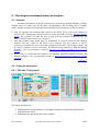
Starting and Running the instruments
Customizable Ion Probe Software
Version 4.0
EdC/ June 2003
The IMS 1270 CIPS 4.0 user's guide (1)
2/83
CIPS User's Manual (1), June 2003, not fully documented for the section Other Analysis
CONTENTS
end of contents
1.
INTRODUCTION............................................................................................................ 6
1.1
1.2
1.3
1.4
2.
THE IMS1270 DOCUMENTATION ................................................................................. 6
ABOUT CIPS ............................................................................................................... 6
THE SERVER ................................................................................................................ 6
CIPS OVERVIEW ......................................................................................................... 8
THE [M,B] TABLE........................................................................................................ 10
2.1
BASICS ...................................................................................................................... 10
2.1.1
The relationship between B and M................................................................... 10
2.1.2
The IMS1270 four mass ranges........................................................................ 11
2.1.3
Computing the magnetic field B after the table [M,B]..................................... 12
2.2
BUILDING-UP AND MODIFYING A [M, B] TABLE......................................................... 12
2.2.1
Overview........................................................................................................... 12
2.2.2
The Main MASS CALIBRATION Panel ........................................................... 13
2.2.3
Initializing the current [M, B] table................................................................. 15
2.2.4
Modifying the current [B, M] table from DISPLAY CALIB............................. 16
2.2.5
Modifying the current [M, B] table from the Mass Calibration program or with
Direct Calib...................................................................................................................... 17
2.2.6
Modifying a [B, M] table from SHIFT CALIB ................................................. 17
2.2.7
Procedure for Calibrating the TOF (Time of Flight)....................................... 18
2.3
THE [M, B] TABLE FILES AND THE SAVE AND LOAD FUNCTIONS............................ 20
3.
STARTING THE INSTRUMENT ............................................................................... 21
3.1
SAVING AND RESTORING KEYBOARD FILES ............................................................... 21
3.1.1
Overview........................................................................................................... 21
3.1.2
The COLUMNS panel ...................................................................................... 21
3.1.3
Starting and stopping the source...................................................................... 23
3.1.4
The source counters ......................................................................................... 23
3.2
THE INSTRUMENT SET-UP PANELS ............................................................................. 23
4.
CHECKING THE INSTRUMENT BEFORE AN ANALYSIS................................. 25
4.1
OVERVIEW ................................................................................................................ 25
4.2
TUNING THE INSTRUMENT ......................................................................................... 25
4.2.1
The main Tuning panel..................................................................................... 25
4.2.2
The Tuning Bargraph panel ............................................................................. 28
4.2.3
The Scan parameter panel................................................................................ 29
4.3
CHECKING THE MASS RESOLUTION AND THE PEAK FLATNESS ................................... 31
4.3.1
Defining and performing a High Resolution spectrum .................................... 31
4.3.2
Featuring a High Resolution Mass Spectrum with the "Peak Processing" ..... 32
4.4
MULTICOLLECTION CASE: SETTING THE TROLLEY POSITIONS .................................... 36
4.4.1
Introduction: The distance/mass multicollector metrology ............................. 36
4.4.2
The Multicollection Tuning panel .................................................................... 37
4.4.3
The Multicollection Control dialog box ........................................................... 38
4.4.4
The Multicollection Control Compute box....................................................... 40
4.4.5
The Multicollection Center Trolley panel ........................................................ 41
EdC/ June 2003
The IMS 1270 CIPS 4.0 user's guide (1)
3/83
4.4.6
5.
The Collector Position Calibration process..................................................... 42
DEFINING AND RUNNING AN ISOTOPE ANALYSIS ......................................... 43
5.1
OVERVIEW ................................................................................................................ 43
5.2
DEFINING AN ISOTOPE ANALYSIS ............................................................................... 44
5.2.1
Overview........................................................................................................... 44
5.2.2
The ANALYSIS DEFINITION panel ....................................................................... 45
5.2.3
Analytical parameters ...................................................................................... 46
5.2.4
The SPECIES TABLE box..................................................................................... 48
5.2.4.1 The species table in the monocollection mode............................................. 48
5.2.4.2 The species table in the multicollection mode ............................................. 50
5.2.4.3 The ratio defining box .................................................................................. 51
5.2.5
The additionnal ISOTOPE boxes ..................................................................... 52
5.2.5.1 Overview ...................................................................................................... 52
5.2.5.2 The Isotopes box: Analysis time, Cycles, Blocks ........................................ 53
5.2.5.3 Isotope analysis option (2): Pre-sputtering................................................... 54
5.2.5.4 The isotope analysis options (3): Reference signal...................................... 54
5.2.5.5 The isotope analysis options (4): Mass calibration Control......................... 54
5.2.5.6 The isotope analysis options (5): Sample HV Control................................. 56
5.2.5.7 The isotope analysis options (6): Overlapping crater................................... 59
5.2.5.8 The isotope analysis options (7): EM drift Control...................................... 59
5.2.5.9 The isotope analysis options (8): Beam Centering....................................... 60
5.3
CALIBRATING THE MAGNETIC FIELD BEFORE THE ANALYSIS ..................................... 60
5.3.1
Introduction...................................................................................................... 60
5.3.1.1 The mass calibration issue............................................................................ 60
5.3.1.2 The M-B memory effect............................................................................... 60
5.3.1.3 The cycling strategy ..................................................................................... 61
5.3.1.4 The ANALYSIS MASS CALIBRATION [m, b] table.................................... 61
5.3.1.5 Monocollection and Multicollection analyses.............................................. 61
5.3.1.6 Manual, semi-auto and auto Mass Calibration modes................................. 62
5.3.2
Analysis Mass Calibration Overview............................................................... 62
5.3.3
Manual Mass calibration ................................................................................. 63
5.3.3.1 The Analysis MASS CALIBRATION panel................................................... 63
5.3.3.2 The Manual MASS CALIBRATION panels .................................................. 66
5.3.3.3 The manual Mass Calibration process ......................................................... 67
5.3.4
Semi auto mass calibration .............................................................................. 67
5.3.4.1 Overview ...................................................................................................... 67
5.3.4.2 The Semi-Auto MASS CALIBRATION panels-1: The main window .......... 68
5.3.4.3 The Semi-Auto MASS CALIBRATION panels-2: The graphic window ...... 69
5.3.4.4 The Semi-Auto MASS CALIBRATION panels-3: The mass calibration table
70
5.3.4.5 The semi-auto mass calibration process....................................................... 71
5.3.5
Automatic mass calibration................................ Error! Bookmark not defined.
5.4
RUNNING AN ANALYSIS ............................................................................................. 72
5.4.1
Running a single analysis................................................................................. 72
5.4.1.1 Overview ...................................................................................................... 72
5.4.1.2 The main Analysis Control panel ................................................................. 73
5.4.1.3 Other windows attached with the Analysis Control..................................... 74
5.4.1.4 The analysis process..................................................................................... 74
5.4.2
Running chained analyses................................................................................ 76
EdC/ June 2003
The IMS 1270 CIPS 4.0 user's guide (1)
4/83
5.4.2.1
5.4.2.2
5.4.2.3
6.
Overview ...................................................................................................... 76
The chained analysis definition panel .......................................................... 77
The chain analysis control panel .................................................................. 78
OTHER ANALYSIS ...................................................................................................... 79
6.1
6.2
6.3
6.4
6.5
OVERVIEW ................................................................................................................ 79
DEPTH PROFILE ......................................................................................................... 80
ENERGY SCANNING ................................................................................................... 80
LINESCAN .................................................................................................................. 81
MASS SPECTRUM....................................................................................................... 82
7.
(DISPLAYING AND PROCESSING THE ISOTOPE ANALYSIS RESULTS)..... 83
8.
(THE EM CONTROL AND EM DRIFT CORRECTION) ....................................... 83
9.
(THE STAGE NAVIGATOR (HOLDER)) .................................................................. 83
10.
(IMAGE PROCESSING) .......................................................................................... 83
11.
(TOOLS) ..................................................................................................................... 83
12.
(APPENDICES).......................................................................................................... 83
12.1
12.2
12.3
12.4
12.5
12.6
(APPENDIX 1: THE EM PHYSICAL PRINCIPLES) ......................................................... 83
(APPENDIX 2: THE EM DRIFT CORRECTION PRINCIPLES) .......................................... 83
(APPENDIX 3: THE QSA EFFECT)............................................................................... 83
(APPENDIX 4: THE FARADAY CUP MEASUREMENT PRINCIPLE).................................. 83
(APPENDIX 5: FUNDAMENTAL OF STATISTICS) .......................................................... 83
(APPENDIX 6: LABVIEW® GRAPH OPTIONS AND GRAPH CURSORS).......................... 83
end of contents
Contents ↑
EdC/ June 2003
The IMS 1270 CIPS 4.0 user's guide (1)
5/83
1. Introduction
1.1 The IMS1270 documentation
The IMS1270 documentation consists of:
The IMS 6F/ IMS 1270 User's guide
The IMS1270 dedicated keyboard user's manual, version 98-1
The IMS1270 ion optics User's manual, version 96-1
User's guide for Multicollector release 1.1
IMS6f/1270 Maintenance guide
National Instruments LabVIEW® User Manual
This CIPS user's guide consists of 3 parts
(1) Starting and Running the instruments (This document)
(2) Processing and tools
(3) Appendices
1.2 About CIPS
The CIPS software has been developped by Cameca under the LabVIEW®
environment (From National Instruments) . It is mainly oriented towards geological
applications and isotope ratio analysis.
The LabVIEW® user manual is a part of the documentation delivered with the
LabVIEW full development version required for the IMS 1270. CIPS users must read the
Chapter 16 Graph and Chart controls indicators. Some pages of this manual are copied in the
appendix LabVIEW® graph options and graph cursors in the third part of this CIPS user's
guide.
Starting CIPS
• Login
• Display the openwindows menu (click in the blue background) and select CIPS (A window
CIPS is then opened)
• Answer Yes to the 2 questions which are asked along the installation of CIPS :
"Do you want to use the back-up holder file ?"
"Do you want to use the back-up calibration file ?"
CIPS scrash
If the program is frozen, type Ctrl C in the CIPS window
Restart CIPS as explained above.
Contents ↑
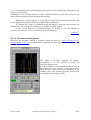
1.3 The Server
Both SUN workstation and microprocessor tasks can communicate between
themselves by the mean of a UNIX mailbox process called IPC (Inter Process
Communication). The so-called ServerSun program insures the message transfer between the
SUN workstation and the microprocessor.
EdC/ June 2003
The IMS 1270 CIPS 4.0 user's guide (1)
6/83
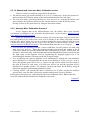
Some communication problems may result in server troubles. Possible error messages
are:
• Server generic error Continue or Stop. It is Highly recommended to click Continue.
• Server Timeout
If some CIPS applications are still scrashed, try to click the small button displayed in
the main menu bar, between TOOLS and Exit.
If clicking the small button fails to re-start the server, open a server window by
clicking server in the openwindows menu and type Ctrl C in this window.
Contents ↑
EdC/ June 2003
The IMS 1270 CIPS 4.0 user's guide (1)
7/83
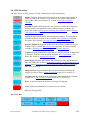
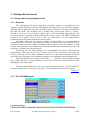
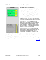
1.4 CIPS Overview
The main menu of CIPS consists of a bar containing the following buttons:
Holder ,Program dedicated to the control of the sample stage motion. It
allows to edit, to save and to recall locations of a given sample holder.
refer to the CIPS user's manual (2), section § The stage navigator
(Holder)
Columns Program dedicated to the ion optics save and restore functions.
It allows also to run automatic source start and stop procedures. See
below the sections § Saving and restoring Keyboard files and § Starting
and stopping the source
Tuning Program dedicated to the instrument setting on, in combination
with the keyboard. It allows also to call the Mass Calibration program.
See below the section § Checking the instrument before an analysis
Analysis Definition Program dedicated to the edition of analysis recipes.
It allows also to call the Mass Calibration program. See the hereunder
sections § Defining an isotope analysis and § Other analysis.
Acquire Program dedicated to run analyses. Analysis results are displayed
in real time. It allows also to call the program Mass Calibration . See
below the section § Running an analysis.
Data Paging Program dedicated to the processing of the output analysis
data. See below the sections § Checking the Mass resolution and the peak
flatness and § Displaying and processing the Isotope analysis results in
the user's manual (2).
Image Process Program dedicated to the processing of scanning ion
images. See the section § Image Processing in the user's manual (2)
Vacuum, Interface dedicated for displaying and controlling the Vacuum
system. See § The Vacuum synoptics in the user's manual (2)
Reset to be used when the kbd error message is displayed.
Tools Opens the additional Tools menu. See just below.
Exit For closing CIPS
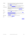
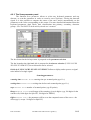
The Tools Bar
EdC/ June 2003
The IMS 1270 CIPS 4.0 user's guide (1)
8/83
Stability
Direct recording and displaying of any primary or secondary signals.
Statistical functions for featuring a recorded stability curve. See the
section § Stability in the user's manual (2)
Set-up
Panels for editing the actual configuration of the implemented hardware.
See the section § The Setup panels in the user's manual (2)
Periodic Table
Displays the Mendeleiev table, allows to select and edit a simple or
compound mass. For a given sample, computes all the interferences at the
neighbourhood af a given mass. See the section § Periodic Table in the
user's manual (2)
PHA
Program dedicated to the record of the EM Pulse Height distribution. See
the section § PHA in the user's manual (2)
Multicol
Opens the Multicollection control panel. See below the section § The
Multicollection control dialog box.
Test
A set of functions for testing and debugging the hardware. See the section
§ Other Tools in the user's manual (2)
More Tools
See the section § Other Tools in the user's manual (2)
Quit
Closes CIPS and Quits
Contents ↑
EdC/ June 2003
The IMS 1270 CIPS 4.0 user's guide (1)
9/83
2. The [M,B] table
2.1 Basics
2.1.1 The relationship between B and M
At a given accelerating voltage (V), the relationship between the magnetic field
(B) and the mass (M) is given by the relationship :
B2 = K * k(B) * M * V
where K is a constant for a given range (see below, § The IMS1270 four mass ranges) given
instrument and k(B) very close to 1 (comprised between 0.96 and 1.04)
At a given accelerating voltage V, approximating k(B) to 1, a single couple values
(M,B) may be used to determine K coarsely, but a single point is not sufficient to mass
calibrate finely the spectrometer. Practically, as high magnetic fields produce non-uniform
pole piece saturation and the magnetic field is measured with a single Hall probe system, k(B)
varies slightly over the B range. Therefore, to be accurate, the mass calibration program
works with a K*k(B) parameter which is mass range dependent.
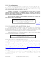
A mass calibration procedure consists of establishing a relationship between a
given mass and the corresponding magnetic field and of storing the values (M,B) in a mass
calibration table.
A mass calibration table consists of :
•
•
•
The secondary accelerating voltage
The secondary polarity.
N values (M,B)i , with 1< i <2000. Mi values are integer numbers.
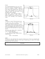
For every mass interval [Mi ,Mj] , Kj is computed following :
Kj = (Bj2 - Bi2) / (Mj - Mi)
Note : every interval width Mj- Mi can be different
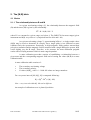
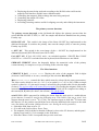
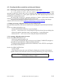
An example of calibration curve is plotted just below
EdC/ June 2003
The IMS 1270 CIPS 4.0 user's guide (1)
10/83
Mass calibration curve (B2 is given in arbitrary unit)
Accelerating voltage : 5 kV
Positive polarity
Kk
1.00
Kk
0.80
B2
Kj
0.60
0.40
Ki
0.20
(M,B)
(M,B) k
(M,B) j
(M,B) i
h
0.00
0
100
Mass
200
300
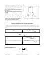
2.1.2 The IMS1270 four mass ranges
The magnetic field B is coded with 19 bits; its maximum numerical value is therefore
524 288. The B numerical value is displayed in the Tuning panel if the B field option is
selected, instead of Mass. Four mass ranges can be manually switched on the magnet power
supply chassis, located at the back of the instrument, underneath the coupling line. At a
secondary voltage of 10KV, these 4 mass ranges correspond respectively to M=300, M=150,
M=75 and M=40. In other words, if the range R300 is selected, the maximum value 524 288
corresponds approximatively to the Mass 300 a.m.u, at 10KV, and to the mass 600 a.m.u at
5KV.
The range R300 is the more commonly used. Other mass ranges are selected
whenever an analysis requires only low mass measurement at high resolution. For example,
let us suppose that the largest mass range, R300, is selected with a secondary voltage of 5KV.
The full scale, 524 288 corresponds to M=600, and M=17 will be obtained for B=88250. In
this case, an increment of one digit will lead to a relative mass increase of 23 ppm. Such a
resolution is not sufficient to center a flat top peak at a mass resolution of 6000 (See the
IMS1270 ion optics user's guide). The operator must then switch to a lower mass range,
according to the higher mass to be analysed.
A given [M, B] table is suited for a given configuration (Mass range, Sec Voltage)
Whenever the user either switches the mass range or modifies the Sample HV, he must
load the corresponding [M, B] table.
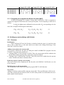
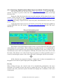
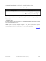
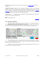
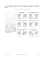
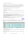
The following table gives the relationship between the hardware Mass Range, the
sample HV and the measurement displayed on the Hall probe Voltmeter (located on the
measurement chassis front panel).
EdC/ June 2003
The IMS 1270 CIPS 4.0 user's guide (1)
11/83
Mass Range R1
Mass Range R2
Mass Range R3
Mass Range R4
Sample HV=10KV
M = 300 Vhall = 10
M = 150 Vhall = 5
M = 75 Vhall = 2.5
M = 40 Vhall = 1.33
Sample HV=9KV
M = 333 Vhall = 9
M = 167 Vhall = 4.5
M = 83 Vhall = 2.25
M = 44 Vhall = 1.20
Sample HV=5KV
M = 600 Vhall = 5
M = 300 Vhall = 2.5
M = 150 Vhall = 1.25
M = 80 Vhall = 0.67
Contents ↑
2.1.3 Computing the magnetic field B after the table [M,B]
In different programs, for example, Tuning, Mass Calibration, CIPS is requested to
compute the magnetic field B from the current [M, B] table. The B computing is achieved as
follows:
Let Mk the highest mass calibrated in the mass table. Bx corresponding to the the
mass Mx is computed following the relationship :
if Mx ∈ [Mi , Mj]
Bx2 = Kj (Mx - Mi) + Bi2
(3)
if Mx > Mk
Bx2 = Kk (Mx - Mk) + Bk2
(4)
2.2 Building-up and modifying a [M, B] table
2.2.1 Overview
Initialization
When clicking INIT, the [M, B] table is initialized with the point (0, 0) and the point
(Mrange, Bmax), where Mrange is the mass which was edited in the editing field Range of the
main Mass Calibration panel .
Adding a new point to the current table
A new point is added into the table by calling the MASS CALIBRATION program from the
TUNING. 2 cases are to be considered:
• Clicking DIRECT CALIB from the TUNING. Then, the current point (M, B) is added to the
[M, B] table without opening Mass Calibration program windows.
• Clicking CALL CALIB from the TUNING. Then, the point will be added after the operator
clicks VALID in the Mass Calibration Panel.
Removing a point from the current table
This can be achieved by displaying the [M, B] table with DISPLAY CALIB and to use the
Delete function.
Modifying the overall current table
The overall table can be shifted by using the program SHIFT CALIB function.
Save/Load
Adding or deleting a point modifies only the current table. These modifications will be saved
only if the operator uses the function SAVE. It will be then possible to recall further the saved
table with the LOAD function.
EdC/ June 2003
The IMS 1270 CIPS 4.0 user's guide (1)
12/83
The overall Mass Calibration program is presented in the section § Defining and
Running an Isotope Analysis, subsection § Calibrating the magnetic field before the analysis.
Contents ↑
2.2.2 The Main MASS CALIBRATION Panel
SAMPLE HV , DISPLAY Field, is the sample HV which was recorded in the current [M, B]
table file when it was created.
POLARITY , DISPLAY Field, is the sample HV polarity which was recorded in the current
[M, B] table file when it was created.
MASS RANGE, DISPLAY Field, is the Mass Range, recorded in the current [M, B] table
file and corresponding to 524288 digits.
Mass and Bfield, DISPLAY Fields, display the current Mass and Bfield.
MRP, EDIT/DISPLAY Field, is initialized as the Analysis Mass Resolution MR if the mass
calibration routine is called from Analysis or the last used value if it is called from Tuning. It
can be also be edited by the operator and will then determine the scan width (See the
hereunder section § Calibrating the magnetic field before the analysis) .
Set calib detector (EM/FC1/FC2/L'2/L2...)
Calibration.
selects the detector involved in the Mass
CYCLING (TAGGED/NOT TAGGED) selection: If CYCLING is tagged in blue, that means that the
B field is always controlled under the current analysis cycle, with the actual analysis timing.
No calibration can be achieved in this mode.
EdC/ June 2003
The IMS 1270 CIPS 4.0 user's guide (1)
13/83
DISPLAY CALIB allows to display the current [M, B] table and to delete one or several
point if required. See the hereunder section § Modifying a [M, B] table from DISPLAY
CALIB.
SHIFT CALIB
allows to shift the overall [M, B] table. See the hereunder section §
Modifying a [B, M] table from SHIFT CALIB
CALIB TOF allows to display and to build the table [M, TOF]. See the hereunder section §
Procedure for Calibration the TOF (Time of Flight)
MASS CAL. MANUAL allows to perform a manual calibration and opens the corresponding
dialog box. See the hereunder section § Manual Mass Calibration
MASS CAL.SEMI-AUTO allows to perform a semi-auto calibration and opens the
corresponding boxes. See the hereunder section § Semi-Auto Mass Calibration .
CENTER TROLLEYS Is used for the multicollector, once a given mass peak has been
adjusted with respect to the corresponding detector, it allows to center mechanically the other
moving detectors with respect to other ion peaks. See the hereunder section § The
Multicollection Center Trolley Panel .
CALIB.FROM TABLE/ CALIB FROM CONDITIONS This selection is used only when
the Mass Calib is called from Analysis definition. Whenever CALIB FROM TABLE is selected
the initial Bfield corresponding to each mass is derived from the [B, M] table. Whenever
CALIB FROM CONDITIONS is selected the initial Bfield comes from the analysis [m, b]
table. See the hereunder section The Mass Calibration [m, b] table
FILE NAME DISPLAY Field displays the current [M, B] table filename.
QUIT closes the Mass calibration window.
File (load/ save/ save as/ Init new file/Init new file /file info allows to load and save a [M,B]
table. See the next hereunder panel.
Load allows to load a previously stored [M, B] table file. The loaded table becomes the
current [M, B] table. If the Sample HV, the secondary polarity and the Mass Range do not fit
the instrument current status, an error message appears.
Save, Save as allows to save the current [M, B] table. If the current [M, B] table has not yet
been saved, it will not be lost in case of a computer crash and will be backed up providing
that the operator answers "yes" when the software is restarted.
Init New File is used for initializing a new [M, B] table. It activates the reading of SAMPLE
HV, SECONDARY POLARITY and MASS RANGE. MASS RANGE is not read from the hardware but
from the set-up. After the reading, these 3 fields can be edited as well.
EdC/ June 2003
The IMS 1270 CIPS 4.0 user's guide (1)
14/83
File Dialog box
For K_TOF and T_TOF, See the hereunder section § Procedure for Calibrating the TOF
(Time of Flight)
Calibration_datas are purposed for the [B, M] initialization.
Contents ↑
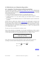
2.2.3 Initializing the current [M, B] table
• Click File/Init new file in the main Mass Calibration panel. Sample HV, Secondary
Polarity, are then read in the General Set-up panel (See the section § The instrument Set-up
panels) and displayed in the fields located in the main Mass Calibration panel.
• If required, edit modifications of the sample voltage and of the range fields. It is a way for
modifying the General Set-up panel.
• It is recommended to calibrate (DIRECT CALIB, from the Tuning) a real mass close to the
upper limit of the range, and then to delete the second default point which was created by
the table initialization.
• Save the file.
Contents ↑
EdC/ June 2003
The IMS 1270 CIPS 4.0 user's guide (1)
15/83
2.2.4 Modifying the current [B, M] table from DISPLAY CALIB
Click DISPLAY CALIB in the main Mass Calibration panel. The graphic window DISPLAY
CALIBRATION is then opened.
3 curves are displayed in the graphic window. The Y-scale is in B2, so that the points
(M,B) are on a striaght line in a first approximation.
• The [M,B] curve, segment_interpolate, consisting of the actual table points, and linear
interpolation between these points.
• The line Best linear fit, which fits as close as possible the actual curve [M, B]
• The difference between the first 2 curves, error, targetted to point out an spurious point (for
such a point, the difference between the 2 curves is expected to be far larger than for the
other points.)
2 cursors are available: a yellow cursor Del used for deleting a point and a green
cursor Mass dedicated to the diplay of the exact values in the display fields current Mass and
B field.
LIN/LOG allows to change the scale. Note that there is no reason to use a LOG scale
UNDO allows to restore the point which has just been deleted
Delete + VALID allows to delete a point of the [M, B] curve: put the yellow cursor Del onto
the point to be deleted, and click Delete. (The Del cursor option must be Snap to point)
Contents ↑
EdC/ June 2003
The IMS 1270 CIPS 4.0 user's guide (1)
16/83
2.2.5 Modifying the current [M, B] table from the Mass Calibration program or
with Direct Calib
Adding a new point or modifying a previous registered point requires to use the
function DIRECT CALIB (See the hereunder section § The main Tuning panel) or to call the
program Mass Calibration from the tuning.
DIRECT CALIB is the easiest way for adding a point to the [M, B] table: Set the Mass M in
the Tuning Panel. Set the B field by using the keyboard Mass thumbwheel (The actual value
of B is then displayed in the Tuning panel). Then click DIRECT CALIB
CALL CALIB can be used as well. It opens the main Mass Calibration panel. It is then
required to use the Mass Calibration program. See the sections § The Manual MASS
CALIBRATION panels and § The Semi-Auto MASS CALIBRATION panels. A (M, B) point is
added or modified in the current [M, B] table when clicking ALL DONE.
When using the Mass Calibration program from Analysis Def or from Analysis, the calibrated
values of B are directly included in the current analysis mass table, but not registered in the
[M, B] table.
Contents ↑
2.2.6 Modifying a [B, M] table from SHIFT CALIB
The SHIFT CALIB function allows to transform the current [M, B] table
according to the relationship
Bi(new) = Bi(old) x Bref(new) / Bref(old)
Where Bref(new) is the current B field value and Bref(old) is the value of B corresponding in
the previous [M, B] table to the current Mass, as it is displayed in Tuning.
Procedure
• In the Tuning Panel, set the mass which will be used as reference and set the B field with
the keyboard thumbwheel.
• Click CALL CALIB.
• In the main Mass Calibration Panel, click SHIFT CALIB.
• A small box is then opened in the Mass Calibration panel, allowing to select the mass
range the shift operation will be applied on. In this small box, if OVER RANGE is selected,
the shift will be applied for the overall table. If IN THE RANGE is selected, the shift
transformation will be applied only between Low Mass and High Mass, contained in the
small box editing fields.
• In the graphical window, click DO+VALID.
EdC/ June 2003
The IMS 1270 CIPS 4.0 user's guide (1)
17/83
The SHIFT CALIB Panel
The graphical window which is opened when clicking SHIFT CALIB is identical to the
DISPLAY CALIB graphical window, except that Delete is replaced by DO. UNDO cancels the
last DO action.
Contents ↑
2.2.7 Procedure for Calibrating the TOF (Time of Flight)
As the velocity of ions is not infinite, there is a delay between the primary beam
rastering and the ion detection which must be taken into account to reconstruct scanning ion
images. This delay, called Time of Flight (TOF), depends mainly on the secondary ion mass
and on the secondary voltage:
TOF ( µs ) = 2.285 ∗ L( m) ∗
M ( amu
U ( KV )
L, the distance between the sample plane and the EM, is 6.3m for the IMS1270. This
gives 72 µs at 10KV for the mass 250. This is not negligible for the scanning ion image, since
the pixel time is 2µs at the lower scanning rate and 0.2 µs at the higher scanning rate.
For a given mass, the TOF is determined by tuning the SII image (See The IMS 6F/
IMS 1270 User's guide, section § 6.2 Scanning Ion Image). The TOF calibration makes it
possible to record several points (M, TOF), to deduce the pair of coefficient K_TOF and
T_TOF of the best fitted function
TOF = T_TOF + K_TOF * M1/2
EdC/ June 2003
The IMS 1270 CIPS 4.0 user's guide (1)
18/83
Normally, only 2 points are necessary for determining the pair of coefficients, but
more than 2 points can be recorded and taken into account. The TOF calibration parameters
are saved in and loaded from the same file than the mass calibration table.
Procedure
• On the main Mass Calibration panel, click
• Select the required mass on the Tuning panel, tune B with the keyboard mass thumbwheel.
An EM signal is obtained.
• Adjust the TOF correction value on the SII chassis.
• On the graphical TOF CALIBRATION panel, click ADD + VALID. The TOF calibration
curve is updated (the curve is plotted only after the second point of the curve has been
calibrated).
The TOF CALIBRATION panel
ADD for adding a new point
Delete for deleting a point
VALID must be made before leaving the application for taking into account the
modifications in the current [M, B] table
Contents ↑
EdC/ June 2003
The IMS 1270 CIPS 4.0 user's guide (1)
19/83
2.3 The [M, B] table files and the SAVE and LOAD functions.
The [M, B] files are normally stored in the sub-directory calib
In the main Mass Calibration panel, click File
Save, save as This function saves, on the hard disk, the current [M, B] table. A box is opened.
Type a file name in the file name field. This box can be used as a [M, B] file manager. The
parameters displayed in the main Mass Calibration panel (Secondary Voltage, polarity and
mass range) are saved in the [M, B] file and the TOF coefficients as well. It is recommended
to give an explicit filename (for example neg_9KV_mass70)
Load The [M, B] table file manager box is opened and allows to load the selected [M, B]
table as the instrument current [M, B] table. This loaded table replaces the previous current
[M, B] table (do not forget to save it, if required). The secondary voltage, the polarity and the
mass range are displayed in the main Mass Calibration panel. The TOF coefficients are
loaded as well and replace the previous.
Init New File This function erases the current [M, B] table and creates a new table with 2
points (0, 0) and (Mrange, Bmax) where Mrange is the value displayed in Range, and Bmax=524288
Contents ↑
EdC/ June 2003
The IMS 1270 CIPS 4.0 user's guide (1)
20/83
3. Starting the Instrument
3.1 Saving and restoring Keyboard files
3.1.1 Overview
The configuration of all the instrument parameters which are controlled from the
computer and are normally tuned from the dedicated keyboard can be saved on the computer
disk and restored further by using the COLUMNS panel, available by clicking COLUMNS on
the main bar menu. The keyboard file is divided into several parts: Sources, Primary,
Secondary, Detection, Presets, Motors, which can be saved and loaded independently. The
lists of parameters contained in these different files can be read in The IMS1270 dedicated
keyboard user's manual and in User's guide for Multicollector for the multicollector
parameters saved and loaded with the Detection option.
Practically, when the user wants to change a keyboard file, it is recommended to
perform a Global Download. Normally this operation occurs whenever the main ion optical
parameters (Source, primary voltage, secondary voltage, sample z) must be changed. As long
as these main parameters are constant, the same keyboard file can be used and only Start and
Stop Source operations will be performed.
The partial save and load operations are recommended for Detection concerning the
multicollector which may be not used. Partial save and load operations concerning the
Primary parameters, the Secondary parameters, the Preset or the motor parameters are useful
especially at the first steps of the instrument setting on, for building the main keyboard files.
The keyboard files are normally saved in the ....... directory. All the global keyboard
files contains one type of sources among Cs+/Ga+/O2+/O-/O2-/Ar+ and they will be sorted
depending on this source type.
For more details about the save and restore keyboard file issue, read The IMS1270
dedicated keyboard user's manual, § Appendix7: Saving and Restoring the keyboard files.
Contents ↑
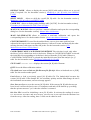
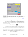
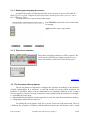
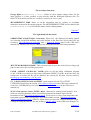
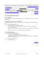
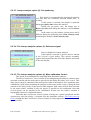
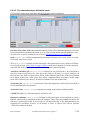
3.1.2 The COLUMNS panel
Left hand side bar
GLOBALS/SOURCES/PRIMARY/SECONDARY/DETECTION/PRESETS/MOTORS
EdC/ June 2003
The IMS 1270 CIPS 4.0 user's guide (1)
21/83
Selects which part of file will be downloaded, or saved or viewed (display of parameter values
on the computer screen).
Global Download includes also a possible start source.
Bottom bar
Cs+/Ga+/O2+/O-/O2-/Ar+/NEG
This bar appears only if the Source button is blue. It selects the source which will be started
or stopped.
Cs+ indicates Cesium Source
O2+ and Ar+ indicates the Duo Source in the positive polarity. The selection O2+/Ar+
implies only a file sorting.
O2- and O- indicates the Duo Source in the negative polarity. The selection O2-/O- implies
only a file sorting.
NEG indicates the Electron Gun
Right hand side bar
DOWNLOAD Restore a saved file and loads the parameters towards the intrument hardware.
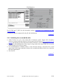
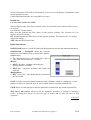
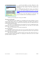
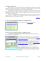
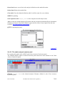
DOWNLOAD + GLOBALS opens the opposite
dialog box. The buttons allow to select some options:
Source (Cs+)
• The download process will include Start Source
only if the source button (Cs+) is blue.
Motors
• MOT is not blue: Nothing concerning the
aperture motors is loaded.
• MOT blue: Apertures positions and width are
restored.
Multicollector
• DET is not blue: The Multicollector parameters
are not loaded.
SAVE saves the current keyboard parameters with a filename edited in a dialog box. A first
dialog box allows to select the type of source which must be associated with the file.
VIEW allows to read (but not to edit) the parameters contained in any stored keyboard file.
Stop source, Start source allows to run the automatic procedure of starting or stopping a
source. A dialog box allows to select the type of source and to delay the Start or Stop
operation.
Contents ↑
EdC/ June 2003
The IMS 1270 CIPS 4.0 user's guide (1)
22/83
3.1.3 Starting and stopping the source
A detailed descrition of both Start and Stop source process is given in The IMS 6F/
IMS 1270 User's guide, Chapter Keyboard functions, section § Duo source files, Cs source
files, NEG source files.
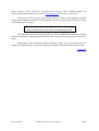
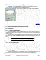
Clicking Stop Source opens the hereafter panel
Cs+/NEG/Duo selects the source which must
be stopped.
Apply runs the source stop routine.
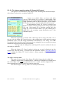
3.1.4 The source counters
This panels is displayed whenever CIPS is opened. The
source status (ON/OFF) are displayed, and for every
source the number of ON hours since the last reset.
Contents ↑
3.2 The instrument Set-up panels
The set-up panels are targetted to configure the software accordingly to the hardware
actually implemented. It is necessary to call and modify the set-up panels whenever the
hardware is modified; Most of these modifications are normally achieved by the Cameca
Service engineers, but the user may also achieve some modifications by himself, for example:
• Switching the mass range
• Mounting different diameter contrast apertures or new slits onto the multicollector trolleys.
• Changing the multicollector detectors.
For calling the set-up panels, click Set-up on the Tools bar of the main menu. There is
3 different Set-up panels, swichable with the button located at the left bottom corner of each
EdC/ June 2003
The IMS 1270 CIPS 4.0 user's guide (1)
23/83
panel: General Set-up/ Hardware Set-up/Detection Set-up. These different panels are
displayed and commented in the section § The Setup panels in the user's manual (2)
On the general Set-up panel, Mass Range (300/150/75/40) is the hardware switching
which can be manually selected at the instrument rear side. It corresponds to different ranges
of the Magnet power supply.
Whenever the operator switches the Mass Range, he
must update the set-up panel corresponding field
Note that both fields Mass Range and Energy can be modified from this panel, but also
from the main Mass Calibration panel (See above the section § Initializing the current [M, B]
table)
Mass Range "300" means that at 10KV secondary voltage, the on axis mass at the exit
magnet will approximatively 300 for the maximum magnetic field maximum value 524 488.
Contents ↑
EdC/ June 2003
The IMS 1270 CIPS 4.0 user's guide (1)
24/83
4. Checking the instrument before an analysis
4.1 Overview
Once the instrument is correctly configured for an analysis (suitable kbd file is loaded,
suitable source is started, the [M, B] table corresponding to the secondary HV is loaded),
before starting an analysis, the operator must check that the instrument is ready for analysis:
• First the operator must obtain some signal on the MCP device and on the main axis
detectors. The Tuning panel will be involved (see the hereunder section § The main Tuning
panel). The operator will then be able to play with the dedicated keyboard (See the
IMS1270 dedicated keyboard user's manual)
• Then the operator must check that the instrument is correctly tuned for the planned
analysis. (See the IMS1270 ion optics User's manual). For this purpose, it will be
necessary to estimate the mass resolution by looking at the MCP video camera image, and
in order to measure it more accurately, by achieving and featuring a High Resolution
Spectrum. (See the hereunder section § Checking the Mass resolution and the peak
flatness).
• In the case of a multicollection analysis, the operator must also position correctly the
moving collectors. (See the hereunder section § Multicollection case: Setting the trolley
positions).
Contents ↑
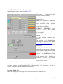
4.2 Tuning the instrument
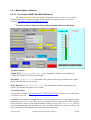
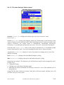
4.2.1 The main Tuning panel
Click Tuning in the main menu bar
The tuning functions are :
¾ Displaying the current primary or secondary intensities in both monocollection and
multicollection modes
¾ Displaying the current B field value (in digits)
EdC/ June 2003
The IMS 1270 CIPS 4.0 user's guide (1)
25/83
¾ Displaying the mass being analyzed according to the B field value read from the
magnetic field interface and the mass calibration table.
¾ Controlling the magnetic field to change the mass being analyzed.
¾ Controlling the sample HV offset.
¾ Displaying polarities
¾ Activating centering routines useful for aligning correctly and reliably the instrument.
The primary current functions
The primary current bargraph, at the left hand side diplays the primary current when the
switch BEAM ON/OFF is OFF (i.e. OFF the sample and therefore blanked into the primary
Faraday cup.
IONS OFF/ ON This switch is the image of the Beam ON/OFF key implemented on the
dedicated keyboard. It switches the primary ions onto the sample (ON) or onto the primary
Faraday cup (OFF).
e- OFF/ ON This switch is the exact image of the e- ON/OFF key implemented on the
dedicated keyboard (NEG Electron beam ON or OFF)
Lock OFF/ ON If Lock ON, IONS and e- are switched togeteher ON/OFF. But if IONS
ON/OFF or e- ON/OFF is switched from the keyboard, both functions are not linked.
PRIMARY CURRENT (above the bargraph) diplays the numerical value of the primary
current intensity, in Amperes or in cps, according to the selection A/cps
The Mass functions
CURRENT B field DISPLAY Field Displays the value of the magnetic field in digits
(between 0 and 524288) or in a.m.u, according to the selection Mass/B field
Mass EDITING Field controls the Mass which must be selected by the mass spectrometer.
The Mass can be edited in a.m.u (i.e. 161.1) or in symbol (i.e. Cs Si, or 29Si). When a simple
symbol is edited (i.e. Si), the major isotope is selected by the periodic table (See the hereunder
section § The species table in the monocollection mode). For loading the magnetic field on the
instrument, hit Enter on the computer keyboard. The B field will be computed according to
the current [M, B] table (See above, the section § The [M,B] table)
axial/L'2/L2/.../H1 is purposed for shifting the beam from the main axis to a multicollector
given detector. It must be used in the following way. This field is first set to axial. Let's
suppose that the mass is set to 28Si (27.98). The operator targets to shift this 28Si beam onto
the detector L'2 the position on which has been correctly initialized with respect to the main
axis. (See below, the section § Multicollection case: Setting the trolley positions).
• Switch the field from axial to L'2
• Si is still in the field set Mass. Press Enter
• The magnetic field is shifted so that the Si Beam is close to the L'2 detector, and the panel
displays axial and 29.15 (for example) in the field Mass.
• Note that "Direct Calib" corresponds always to the axail case.
EdC/ June 2003
The IMS 1270 CIPS 4.0 user's guide (1)
26/83
The secondary functions
Energy Offset EDITING Field + cursor allows to edit a sample voltage offset. For the
same purpose, it is also possible to play directly with the dedicated keyboard (See The
IMS1270 dedicated keyboard user's manual, section § the source pad)
MEASUREMENT TIME allows to set the integration time for primary or secondary
intensities measured in the tuning program. The MEASUREMENT TIME can be edited in the
DISPLAY/EDITING Field or set with the mouse on the rotating button.
Contents ↑
The right hand side bar menu
CORRECTION ON/OFF/define Corrections When ON, the displayed secondary signals
are corrected for the EM deadtime and yield, defined in the Detection Set-up panel (See the
sections § The EM Physical principles and § Detection Set-up panel in the CIPS user's
manual (2)). Define Correction is a shortcut for editing directly the correction parameters.
MULTICOL/MONOCOL MODE This selection leads to open the multicollection Bargraph
panel or the monocollection Bargraph panel.
CALIB (DIRECT CALIB/CALL CALIB) allows to call the Mass Calibration program
(CALL CALIB) or to achieve a direct mass calibration (DIRECT CALIB). In this last case, the
current pair of values (M, B) will be added to the current [M, B] table. See the section §
Building-up and modifying a [M, B] table.
FC_CALIB: OFFSET/ GAIN & OFFSET opens respectively the FCs OFFSET
CALIRATION panel (See the section § FCs Offset Calibration in the CIPS user's manual (2))
or the FCs CALIBRATION panel (See the section § FCs Calibration in the CIPS user's
manual (2)).
SCAN/ Field Aperture Center/ EM HV Adjust , shortcuts for running useful routines. Scan
allows to scan any parameter and to record any measurement channel ouput (See the
hereunder section § The Scan parameter panel). Field Aperture Center scans and centers the
beam with respect to the Field Aperture (See the hereunder section § The Scan parameter
panel/ Field Aperture Center). EM HV Adjust allows to reajust the Electron Multiplier High
Voltage all along the EM life (See the section § EM HV Adjust in the CIPS user's manual (2))
.
Contents ↑
EdC/ June 2003
The IMS 1270 CIPS 4.0 user's guide (1)
27/83
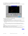
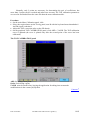
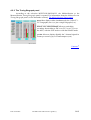
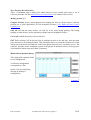
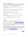
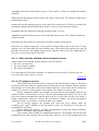
4.2.2 The Tuning Bargraph panel
According to the selection MULTICOL/MONOCOL, the Multicollection or the
Monocollection Tuning Bargraph panel is opened. For information about the Multicollection
Tuning Bargraph panel, see the hereunder section § The Multicollection Tuning panel.
more/ less diplays either simultaneously the 3 EM-FC1FC2 bargraphs (more) or just a single bargraph (less).
EM/FC1/FC2/SLIT/IMAGE allows to switch the
secondary beam either to EM or to FC1 or to FC2 or to
the MCP, with the SLIT mode or with the IMAGE mode.
cps/nA allows to display digitally the 3 channel signals in
counts per seconf (cps) or in nanoamperes (nA)
Contents ↑
EdC/ June 2003
The IMS 1270 CIPS 4.0 user's guide (1)
28/83
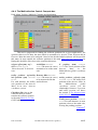
4.2.3 The Scan parameter panel
The function Scan parameter allows to select any keyboard parameter and any
detector, to scan the parameter in order to record a curve S(param), S being the detected
signal. It is also possible to compute the center of the curve and to automatically set the
parameter to the value corresponding to this center. For more detailed information about the
keyboard parameters (their labels, their classification into primary, secondary, detection
groups... See The IMS1270 dedicated keyboard user's manual.
The box located at the left top corner is purposed to the parameter selection
The bar located at the right hand side is purposed to the detector selection (L'2/L2/L1/C/H1
/H2 /H'2/ FC1/EM/FC2). Several detector can be selected.
Divide by L'2/L2/L1/C/H1 /H2 /H'2/ FC1/EM/FC2 allows to diplay and to process a signal
ratio instead of a single signal.
Scanning parameters
counting time EDITING Field counting time per scanned point (typ 0.1 s)
waiting time EDITING Field waiting time before each scanned point (typ 0.1 s)
steps EDITING Field number of scanned points. (typ 50 points)
Range EDITING Field overall range of the scanning, given in digits. (typ, 300 digits for the
entrance slit, 1000 digits for Sple HV, 300 digits for DSP2Y)
Offset EDITING Field the parameter will be set to the computed center of the curve + the
offset (typ 0, except +20 digits for Sple HV)
EdC/ June 2003
The IMS 1270 CIPS 4.0 user's guide (1)
29/83
The lower bar menu
PRINT for printing the graph
LIN/LOG graph scaling option
Center computes the center of the curve Xcenter (The maximum Ymax is firstly computed. Xleft
and Xright, corresponding to the interpolated points such as Y(Xleft)= Y(Xright)=Ymax/2, and
finally, Xcenter = (Xleft+Xright)/2. If several detectors are selected (for the multicollector tuning),
the curve to be computed is selected in the box Center on detector, located just under the
graphical window.
VALID After a center operation, clicking VALID actually sets the parameter center value.
START/RUNNING Clicking START launches the scan. At the end of each scan, the displayed
curves are erased and another scan restarts automatically as long as the user does not click
RUNNING for stopping the scan
Deriv if this button is marked, the derivative will be displayed.
snap Q24 if this button is marked, several scans corresponding to different detector
selections can be displayed in the same graph, providing the same parameter is scanned.
shift If this button is marked, it is possible to display on the same graph several scan,
corresponding to different parameters, providing the same detector is selected. After clicking
shift, the next scan will be saved and displayed. At each shift, the small DISPLAY box at the
right hand side of shift is incremented.
print to file It is possible to save the scan function results in a file. Set print to file to ON
The Field aperture Center case.
When selecting Field aperture Center in the Tuning
panel, 2 full scan & center routines will be achieved over
the parameters purposed to centre the beam within the
Field Aperture, LT1 defatx and LT1 defaty.
The operator is just required to select the detector
channel before the routine is started.
Both initial LT1 defatx and LT1 defaty are displayed in
the field x&y.
Contents ↑
EdC/ June 2003
The IMS 1270 CIPS 4.0 user's guide (1)
30/83
4.3 Checking the Mass resolution and the peak flatness
4.3.1 Defining and performing a High Resolution spectrum
As it was pointed out above (See the section § The main Tuning panel) a mass
spectrum around the current mass can be launched and displayed directly from the main
Tuning panel by clicking SCAN (at the panel right hand side). The displayed spectrum can be
printed, but it cannot be processed.
For being able to process a spectrum and thus to feature a peak (mass resolution,
flatness), it is necessary to launch a High Resolution Spectrum.
The process for running a High Resolution Spectrum is very similar to the Isotope
analysis (See below the section § Defining and Running an isotope analysis)
1. Editing and saving a High Resolution Spectrum definition file
From the main menu bar, click analysis definition for opening the ANALYSIS DEFINITION
box.
In the ANALYSIS DEFINITION box
• Select HIGH RESOLUTION as Acquisition Mode
• in File..., select Load or New for opening the High Resolution Spectrum dialog box.
• Enter the analysis input data (mass, scan parameters...) in the dialog box.
• Select on File... /save or save as for saving the analysis definition file.
2. For running a High Resolution Spectrum
In the ANALYSIS DEFINITION box
• Select the required analysis file
• It is possible to launch the Mass Calibration by clicking CALIBRATE, though it is
generally not required before a High resolution spectrum.
• After the mass calibration (quit the box calibration), click APPLY for opening the
ANALYSIS CONTROL box.
In the ANALYSIS CONTROL box
• Click START
•The High Resolution Spectrum will then be displayed at real time in the analysis
graphic window (See below the section § Defining and Running an isotope analysis)
In the High Resolution Spectrum scanning process, the B
field step is always 1 digit.
Contents ↑
EdC/ June 2003
The IMS 1270 CIPS 4.0 user's guide (1)
31/83
4.3.2 Featuring a High Resolution Mass Spectrum with the "Peak Processing"
The curve browser box (See the section § The curve browser box in the CIPS user's
manual (2)) allows to process either the current acquisition, or a previously saved High
Resolution file.
During the High Resolution Spectrum run, the spectrum will be plotted in the curve
graphic window (See the section § Displaying and processing the analysis results with the
curve panel in the CIPS user's manual (2))
For processing a High Resolution Spectrum peak, click MEASURE in the the curve
graphic window.
A High Resolution Spectrum curve can also be processed by the functions available by
clicking PROCESS (See the section § The curve processing functions in the CIPS user's
manual (2)).
The peak information panel
Each button of the panel bottom assigns cursors to special functions and opens a box
which displays the peak features. When using any processing function, it is recommended to
check that the cursors required for the processing are displayed on the screen. If they are not,
check that the cursor color is not transparent. Normally, the useful cursors can be driven with
the mouse. This feature is set in the Graph Properties panel. It is always possible to move a
cursor by blackening the square in the cursor table and by clicking the special cursor button
All the functions are purposed to feature a single peak. It is thus recommended to set
the graph scale in order to plot a single peak in the graphic window
Intensity
When clicking Intensity, the vertical cursor #0 is automatically positionned at the curve
maximum. It is possible to move the cursor to explore the curve. The (Mass, Intensity) box,
opened at the peak_information panel left hand side displays the coordinates of the curve
current point.
EdC/ June 2003
The IMS 1270 CIPS 4.0 user's guide (1)
32/83
Curs 2 (% max)
Center max
Intensity (cps)
Center
The second left hand side (Center min, Center
max) box is opened. 2 horizontal cursors #1
and #2 are assigned to define 2 different
levels. These levels (default value: 10% and
90% of the maximum) can be tuned by
editing the fields %min and %max or by
moving the cursors manually.
Each cursor peak intersection defines 2
points. The abcsissa of center of these 2
points is displayed in the field Center min or
Center max, according to the considered
cursor
Curs 1 (% min)
Center min
X(a.m.u.)
Curs 6 (% max)
Wmax
Curs 5 (% min)
Wmin
Intensity (cps)
Width
A third box is opened. The horizontal cursors
#5 and #6 are used for defining 2 levels
editable in the fields %min and %max.
The 2 display fields located below WIDTH
contains the respective peak width Wmin and
Wmax corresponding to the respective cursors
min and max. Wmin and Wmax are expressed
in ppm.
The delta (ppm) display field is intended to
feature the peak edge width:
delta= (Wmin+Wmax)/2
The Mass Resolution MRP (display field) is
related to Wmin
MRP= 1 000 000/Wmin
X(a.m.u.)
FLAT
The last box, at the right hand side is opened. Vertical Cursors #7 #8 #9 are assigned to this
peak flat top featuring. Cursor #8 is the center of both cursors #7 and #9. It is firstly
positionned at the curve maximum.
FLAT is dedicated to feature the part of the peak top located between the cursors
#7 and #9
EdC/ June 2003
The IMS 1270 CIPS 4.0 user's guide (1)
33/83
Intensity (cps)
Cursor 9
Cursor 8
dM/M
Cursor 7
The distance between both cursors #7 and #9
is the value displayed in the dM/M (ppm)
field. This field can be edited. The cursors can
also be moved manually.
Mean (display field) is the mean intensity of
the peak top.
Mse (display field) is the noise in the peak top
interval.
The flat top is approximated by a straight
segment which is displayed in the graph.
dI/I (%)(display field) is the difference of
intensities between the 2 ends of this segment.
Relative slope is the slope of this segment
Rms is the noise around this segment.
For a more detailed presentation, see below.
X(a.m.u.)
Detailed calculations of the the peak top features
N points are selected between the two cursors. Each point is considered as a pair of
coordinates (Mi, Ii) where Mi is the mass number of the measured point i and Ii the recorded
signal.
Mean
Mean =
I
=
i= N
Ii
∑N
i =1
=
M
i= N
∑
i =1
Mi
N
Mse
1
 i=N ( I − I )2  2

Mse =σ = ∑ i
N
 i =1

dM/M (ppm)
dM / M ( ppm)
= 106
M N − M1
M
Reduced coordinates (mi, si)
EdC/ June 2003
mi
=
si
=
Mi − M
M
Ii
I
The IMS 1270 CIPS 4.0 user's guide (1)
34/83
A regression linear function is calculated for fitting the N peak top points
s = α
m +
β
dI/I(%)
dI/I = 100 α(mN-m1)
Relative slope
Relative slope = α
Rms
1
σ ' 1  i = N (( I i − si ) I − I ) 2  2

Rms =
=  ∑
N
I
I  i =1

It is actually considered that the spread among the intensities Ii is generated by two
phenomenas:
- A linear drift.
- A stochastic effect.
dI/I and the "Relative Slope" correspond to the linear drift while Rms is the standard deviation
once corrected from the linear drift.
NOISE displays 2 parallels segments parallels to the flat top approximated segment,
corresponding to the noise level and distant of 1σ from the flat top segment.
Contents ↑
EdC/ June 2003
The IMS 1270 CIPS 4.0 user's guide (1)
35/83
4.4 Multicollection case: Setting the trolley positions
4.4.1 Introduction: The distance/mass multicollector metrology
The multicollector metrology is initialized by clicking INIT ALL, in the Multicollection
Control box (See below, the section § The Multicollection Control dialog box). For locating
all the detector positions along the trolley axis, in the same coordinate system, the following
data are taken into account:
• 10 mm is the distance between the collector C end stop and the main axis.
• The number of motor step between a given moving collector and its parking stop.
• A Trolley thickness of 5.5 mm, which actually gives the distance between 2 collector
parking stop.
• The Gap between the additionnal detectors L'2 and H'2 and their respective main detector
L2 and H2
All these data are coded in the software, except the Gap which must be entered in the
Detection Set-Up panel. (See the section § Detection Set-up in the CIPS user's manual (2)).
The Gap must be close to 30000. It is equal to the width along the X axis between L2 and L'2
(or between H2 and H'2), in millimeters, multiplied by 2700. The measured width is recorded
in the Multicollector test Sheet (§1.4, Collector thickness: 1-1' and 5-5' are respectively the
L2-L'2 and the H2-H'2 width)
The main axis is the zero of this global coordinate system.
Some of these data have an uncertainty of a few tenth of millimeters, so that, it can be
estimated that the displayed position in the Multicollection Tuning panel have a precision of
±2.5mm along the trolley axis, corresponding approximatively to dM/M=±1/1200
Multicollector Metrology precision:
Trolley axis: ±2.5mm
corresponding Mass Resolution: 600
In the Multicollection Tuning panel, the displayed values of the detector positions are
according to coded hereunder relationship between Mass and detector position :
∆M
 ∆M 
∆X = 1215 ∗
+ 1600 ∗ 

M
 M 
∆Z trolley = 2.7 ∆X
2
Contents ↑
EdC/ June 2003
The IMS 1270 CIPS 4.0 user's guide (1)
36/83
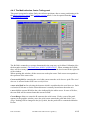
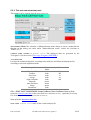
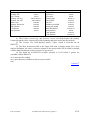
4.4.2 The Multicollection Tuning panel
Select Multicol in the main Tuning panel (See the section § The main Tuning panel)
The trolley position display bar This grey bar, at the top of the window displays the location
of all the detectors. One cursor corresponds to each collector: Blue for L'2-L2, green for L1,
yellow for C, orange for H1 and red for H2-H'2. The black cursor corresponds to the main
axis.
MASS/POSITION If POSITION, the display field above each detector gives in µm the detector
position along the trolley travel axis. If MASS, the display field gives expressed in a.m.u. and
mean the computed mass corresponding to each detector.
MASS RESO./SLIT SIZE If SLIT SIZE is selected, label of the collector entrance slit, as it was
entered in the General set-up panel (See the section § General Set-up in the CIPS user's
manual (2)). Each slit number is labelled by a value Wslit in microns. If MASS RESO. is selected,
the Mass Resolution, computed as 1215000/Wslit.
Slit #1 /#2/ #3 switches the multicollector exit slits (Standard values are 500µm, 250µm and
150µm)
WARNING: For the same slit position (1/2/3), all the detector slits will be identically
labelled, even if different slit bars are mounted onto the different detectors, and the displayed
corresponding mass resolution will be therefore identical.
CPS/A DISPLAY Field displays for each detector the measured signal, in cps or in A
Contents ↑
EdC/ June 2003
The IMS 1270 CIPS 4.0 user's guide (1)
37/83
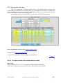
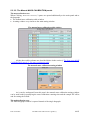
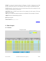
4.4.3 The Multicollection Control dialog box
Open this panel from the main menu Tools bar .
This panel is dedicated to the
movable collectors control
Init will measure the total travel of
all the trolleys.
MARK The checkboxes, at the left
hand side display the proximity with
other collectors (each movable
collector is equipped with an
electrical proximity stop.)
CURRENT
POSITION
(µm)
DISPLAY
Field
The trolley
position is expressed with respect to
its own origin.
Each trolley origin is its parking
position.
All the absolute positions are
positive.
The position in the Multicollector
metrology is displayed only in the
Multicollection Tuning panel and
not in this Multicollection Control
dialog box,
(GO TO) VALID Checkboxes are
purposed for selecting the collectors
which will be actually moved when
Clicking Go to Position or Go to
relative . The GO TO editing fields
close to the checkboxes corresponds
to the position if it is planned to
click Go to Position or just to the
distance to be run if it is planned to
click to Go to relative .
Go to Position, Go to Relative
Activates the motion corresponding to the position or the distance which must be edited
previously (in µm) in the column "GOTO". When pressing "Go to position" or "Go to
relative", only the "VALID" channels will be moved.
Low Mass, High Mass
Useful for setting the correct sign of "relative position" in the fields GO TO .
EdC/ June 2003
The IMS 1270 CIPS 4.0 user's guide (1)
38/83
Store Position, Recall Position
These 3 commands open a dialog box which allows to store, modify and restore a set of
collector positions. See this Multicollector position library box further in this section.
Modify position Q11
Compute Position opens a panel purposed for helping the user to edit the correct collector
position for a given application. See the hereunder Section § The Multicollection Control
Compute box
Park all will sent the outer trolleys (#1 and #5) at the outer buting parking. The buting
parking of other trolleys are the proximity butings between neighbour trolleys.
Center all send all the trolleys close to the axis
INIT Each collector will be driven from its parking location to its end stop, near the main
axis, and back to the parking location. This procedure allows to record the total travel of each
trolley and to measure each collector in the same global multicollector coordinate system. The
collector positions in this coordinate system are displayed in the Multicollector Tuning panel.
(Note that this routine lasts more than 30 minutes)
Multicollector position library
This single table contains all the
saved configuration.
A collector configuration
corresponds to a line.
Select a line for modifying,
deleting or loading a
configuration
Contents ↑
EdC/ June 2003
The IMS 1270 CIPS 4.0 user's guide (1)
39/83
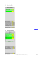
4.4.4 The Multicollection Control Compute box
Path: Menu Tool bar /Multicol /Compute position button
This tool is purposed for finding the collector positions for a given application. The
operator edits in axial Mass the mass which is assumed to be on axis. Then, he must edit in
Detector Mass the mass to be analysed. Once he has decided which collector will be used for
this mass, he may transfer the collector position to the main Muticollection control box by
hitting the checkbox-like close to the considered detector.
ref.pos. offset (µm): ref =
axis EDITING Field
Not to be used. To be set to
zero.
Axial Mass EDITING
Field The mass (in a.m.u.)
assumed to be on the main
axis
trolley position: ref=trolley Detector Mass EDITING
init position (µm) DISPLAY Field The mass (in a.m.u.)
Field
to be measured with the
For each detector, the trolley multicollector.
axis position of the detector
Mass, in its own detector
coordinate system.
Checkbox-like close to the
collector must be used to
transfer the collector postion
to the main Muticol. ctrl box
GOTO table
EdC/ June 2003
X
position (mm) DISPLAY
Field The X axis position of the
detector
Mass,
in
the
Multicollector global coordinate
system.
trolley position: ref=axis (µm)
DISPLAY Field The trolley axis
position of the detector Mass, in
the
Multicollector
global
coordinate system. For the
relationship between X position
and trolley position, see above
the section § The distance/mass
multicollector metrology
Trolley max position: DISPLAY
For each detector, its max
position (close to the main axis,
0 being the parking position..
Contents ↑
Field
The IMS 1270 CIPS 4.0 user's guide (1)
40/83
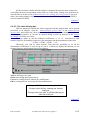
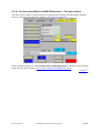
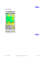
4.4.5 The Multicollection Center Trolley panel
This panel is targetted to adjust finely the collector positions, after a coarse positionning with
the Multicollection control and Compute position panels. It can be opened from the Main
Mass Calibration panel .
The B field is scanned over a range determined in the same way as for Mass Calibration (See
the hereunder section § The Semi-Auto MASS CALIBRATION ). When scanning the B field,
there will be as many spectra as selected (crossed) detectors in the box located at the right side
of the window.
When opening this window, all the cursors are at the plot center. Each cursor corresponds to
the spectrum of the same color.
Center axial field for centering the axial white cursor onto the axial detector peak. The axial
detector is selected in the field center axial field on .
center axial field on for selecting the detector which is considered as the axial detector. Such
a selection is relevant so far the selected detector is actually located near the main axis.
VALID shift the current B field to the value indicated by the white cursor. In case of ReStart,
the scan field will be centered onto this current B field.
Center Range allows to centre the B scan onto the axial cursor. If only a part of the peak
appears in the graphics window, move the axial cursor towards the peak and click Center
range. Nothing will be changed in the [m, b] table, but the peak will be contained within the
B scan.
EdC/ June 2003
The IMS 1270 CIPS 4.0 user's guide (1)
41/83
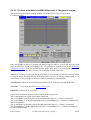
Center Field Automatic centering of each cursor onto the corresponding peak.
Center Trolley Each trolley, if checked in the displacement column, is moved to the position
corresponding to the cursor (The formula X=f(∆M), displayed above in the section § The
distance/mass multicollector metrology is used for this positionning).
WARNING: Enable Centering, in the right side box, is required to be clicked before Center
Trolley
displacement displays the targetted positions if clicking Center Trolleys. Checkboxes are for
validating the trolleys which would be actually moved.
Compute displacement displays in the columns the positions which will be targetted if
clicking Center Trolleys.
Set Trolleys (load position from file/ save position to file/ compute position) opens the
Multicollector position library box for load position and save position, and opens the
Compute position box in the last case.
Back
After clicking Center Trolley, Back recalls the previous trolley positions.
Abort displacement aborts the moving in progress.
Contents ↑
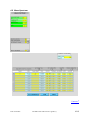
4.4.6 The Collector Position Calibration process
In a simple case, all the masses are measured simultaneously, at the same fixed
magnetic field. In the more general case, the multicollection analysis definition contains
several subsets of masses required to be analysed at the same step of the magnetic field cycle.
1st Case: All the masses are measured simultaneously
The operator must first achieve a coarse positionning with the help of the
Muticollector Tuning panel, the Multicollection Control dialog box and the Multicollection
Control Compute box.
• In the main Tuning panel, set the Mass (or the B field) corresponding to the main axis.
• In the Muticollector Tuning panel, it is possible to view the coarse detector positions,
measured either in microns, or in amu, providing that the metrology initialization has been
previously achieved (INIT in the Multicollection Control dialog box).
• In the Main Tool bar menu, click MULTICOL for opening the Multicollection Control dialog
box.
• In the Multicollection Control dialog box, click compute pos for computing the collector
required positions.
• For each detector, the mass to be measured may be entered, and the Compute box
computes the trolley position which can be transferred in the Multicollection Control
dialog box.
Once the coarse positionning is achieved, the operator must launch the Multicollection Scan
routine in order to get a fine positionning.
• From the main Tuning panel, click CALL CALIB for opening the Mass Calibration panel .
EdC/ June 2003
The IMS 1270 CIPS 4.0 user's guide (1)
42/83
• Set MRP. Taking into account that the coarse positionning precision corresponds to
∆M/M=±1/1200, It is recommended to set MRP to 600 in order to get all the peaks within
the scanning field.
• Click TROLLEY CENTER for running the scan and opening the Multicollection Trolley
Centering panel.
• Select the detectors which must be calibrated in this run.
• Shift the cursors onto their peaks, accordingly to the guidelines described in the above
section § The Multicollection Center Trolley panel.
• Move the trolleys to the cursor positions by clicking Center Trolley.
• Then increase the MRP, and TROLLEY CENTER again.
General case: The Multicollection analysis is achieved in a magnetic field switching
mode.
Then, all the masses to be measured are divided into subset, each subset corresponding to the
same magnetic field. Each subset masses will be measured simultaneously. It must be clear
that during the analysis, only the magnetic field will be switched, while the collectors are not
allowed to move. So, the procedure in this general case is the following:
• Set the positions of the first subset detectors, accordingly to the above described first case.
• Set the positions of the second subset detectors in the same way
• etc...
WARNING: If the same detector is used in several subsets, move it only at the first subset
calibration. At further steps, a magnetic field tuning must be used for centering this detector
peak.
Before running a switching mode multicollection analysis, a Mass Calibration
must be performed, accordingly to the guidelines given below in the section §
Calibrating the magnetic field before the analysis.
Contents ↑
5. Defining and Running an isotope analysis
5.1 Overview
For measuring isotope ratios of a given sample with the monocollection mode, the
operator must have first edited an analysis definition file which contains the input data of an
analysis: Species to be analysed, counting time for each species, ratios which are normally
computed etc... This is described below in the hereunder section § Defining an isotope
analysis.
Let us suppose that the instrument is started and tuned as it was explained above in the
sections § Starting the instrument and § Checking the instrument before an analysis
Before running an analysis, it is first necessary to carry the right point of the right
sample at the good location, at the cross point of both primary and secondary axis. (see § The
Sample Holder and Navigator in the user's manual (2))
Then the operator will recall the analysis definition file if it is not the current analysis
file, and normally, so far the analysis requires high mass resolution, it will be necessary to
achieve a mass calibration in order to assign a precise magnetic field to each species. Due to
EdC/ June 2003
The IMS 1270 CIPS 4.0 user's guide (1)
43/83
the magnet hysteresis, this operation must normally be repeated each time the instrument is
out of the cycle of the analysis. See the hereunder section § Calibrating the magnetic field
before the analysis .
The instrument is then ready for starting an analysis. see below the section § Running
an analysis.
The analysis produces an output data file. For obtaining relevant results, the user can
use some processing facilities such as the isotope spreadsheet . See the section § Processing
the results with the isotope spreadsheet in the user's manual (2).
Contents ↑
5.2 Defining an isotope analysis
5.2.1 Overview
The operator may edit an analysis definition file for running it later or for running it
immediately.
Editing and saving an analysis definition file
From the main menu bar, click analysis definition for opening the ANALYSIS DEFINITION
box.
In the ANALYSIS DEFINITION box
• Select ISOTOPES as Acquisition Mode
• Click EDIT LAST CONDITIONS or Load Conditions or New for opening the
Species Table dialog box.
• Enter the analysis input data (masses, counting time...) in the Species Table dialog
box.
• Click on save or save as for saving the analysis definition file.
For running an analysis
In the ANALYSIS DEFINITION box
• Select the required analysis file
• Launch the mass calibration by clicking CALIBRATE
• After the mass calibration (quit the box calibration), click APPLY for opening the
ANALYSIS CONTROL box.
In the ANALYSIS CONTROL box
• Click START
Contents ↑
EdC/ June 2003
The IMS 1270 CIPS 4.0 user's guide (1)
44/83
5.2.2 The ANALYSIS DEFINITION panel
This pannel can be opened from the main menu bar.
MULTI/MONO Mode The selection of Multicollection mode allows to select a multicollector
detector in the dialog box table while "Monocollection mode" restrict the selection to
"EM/FC/FC2"
SAMPLE NAME, SAMPLE X DISPLAY Field. The displayed data are generated by the
"Navigator" (See the section § The stage Navigator (HOLDER))
ANALYSIS TYPE
It selects the suitable dialog box, according to the analysis, and filters the displayed files
according to selected acquisition mode
Avalaible acquisition modes
Depth profile
isotopes
lines scan
energy
high resolution
bargraph
mass spectrum
image
Parameters
Mono/
Multi
both
both
both
both
both
mono
mono
mono
both
Analysis file extension
.ddp
.dis
.ls
.en
.ddr
.
.
.
File...: EDIT LAST CONDITIONS/ Load Conditions/ Save Conditions/ Save as/ New
opens the SPECIES TABLE box in the cases Edit last conditions or New , opens the file dialog
box in the cases load conditions or save or save as.
New opens the SPECIES TABLE box.
FILE NAME DISPLAY Field
name of the current analysis file
EdC/ June 2003
The IMS 1270 CIPS 4.0 user's guide (1)
45/83
PERIODIC TABLE calls the Periodic table tool. See the section § Periodic table in the user's
manual (2).
Analytical Parameters opens the box Analytical Parameters. The set of Analytical
Parameters gives an overall information of the instrument setting during the analysis. This list
will be included in the analysis output data (See the hereunder section § Analytical
Parameters). Some of them are read on the instrument. Other are entered by the operator.
These last parameters will be attached to the analysis definition.
COMMENTS Edit Field Comments to be attached to the analysis definition file. They will be
printed with the analysis definition field
QUIT
Back to the main menu bar
Contents ↑
5.2.3 Analytical parameters
This table contains editing fields related to the status of the instrument hardware.
Some values are directly read when the button READ is clicked.
WARNING, this program calls a 68030 µP routine which is actually not well-suited to
the IMS1270. Some display fields are irrelevant or wrong (Transfer lens, field aperture)
All these parameters will be included in all the analysis output data files. Some of
them are read and are targetted to record the status of the instrument hardware during the
analysis. Other are filled by the operator.
The analysis does not depend at all on what the operator has written in this box. All of
this information is considered as comments.
EdC/ June 2003
The IMS 1270 CIPS 4.0 user's guide (1)
46/83
Ion Species
Primary HV
Arc Current
Primary cur beg.
Primary cur end
Raster size
Primary beam size
HR aperture
L4 aperture
Duo pressure
EDITED/READ
Edited
READ
READ
MEASURED (1)
MEASURED
EDITED
EDITED
EDITED
EDITED
READ
Sample HV
ESA inner
ESA outer
Transfer lens
Gate DTOS
Gate SII
Entrance slit width
Energy slit width
Mass Resolution
Anal pressure
Cont aperture
Field aperture
EDITED/READ
READ
READ
READ
READ (2)
EDITED
EDITED
EDITED
EDITED
EDITED (3)
READ
EDITED
EDITED (4)
(1) The Primary current beg. and Primary current end fields display the primary
current measured values, respectively at the beginning and at the end of the last analysis.
(2) The Transfer lens field displays always "35µm" which is irrelevant for an
IMS1270.
(3) The Mass Resolution field is the single field with a (slight) action: For a new
analysis definition, the Mass resolution column of the species table will be filled by default
with the Mass Resolution written in Analytical parameters
(4) Not suited for an IMS1270: possible selection is 1/2/3/4 while 5 presets are
available with the IMS1270.
READ activates the reading
SET copies the mass resolution to the new species table
EDIT
Contents ↑
EdC/ June 2003
The IMS 1270 CIPS 4.0 user's guide (1)
47/83
5.2.4 The SPECIES TABLE box
This box is purposed to edit the analysis recipe; The analysis process consists of a
given number of identical cycles. During each cycle, the magnetic field will be swiched to the
values resulting from the mass calibration. Each field step consists of a waiting time targetted
to allow the magnet to settle and a counting time.
All the table fields are editing fields except the Mass ans the B field columns.
GO TO ACQUISITION calls the main Analysis Control panel.
CALIB calls the Mass Calibration panel
CANCEL Closes the panel without saving the modifications.
Contents ↑
5.2.4.1 The species table in the monocollection mode
Main table
All the columns are Edit Field, except the columns Mass and B Field.
A line can be suppressed by deleting the species label and pressing ENTER.
EdC/ June 2003
The IMS 1270 CIPS 4.0 user's guide (1)
48/83
Symbol
Mass
Detector
waiting time (s)
Species to be analysed;
Possible formats:
"130.5" ; then the calculated mass will be 130.5
"Si" ; then the calculated mass will be the Si major isotope exact mass:
27.9769
"30Si2 B" ; then the calculated mass will be 2*29.97649 + 11.00931
"30Si++" ; then the calculated mass will be 0.5*29.97649
The number of atoms for a given species is limited to 99 and a molecular
isotope cannot contain more than 4 different isotopes.
Display Field (the value, in Dalton is calculated as described above)
EM/FC1/FC2
Edit Field If Manual is selected in the Analysis Definition box
Default value 0.5
Display Field If Auto is selected in the Analysis Definition box,
automatically computed according to the formula
∆B
MR
wt =
∗
+ 0 .1
100000
300
An additional waiting time is edited in the right top corner for taking into
account the FC settling time.
Counting time (s) Edit Field
Offset (Volt)
Sample HV voltage offset to be applied for this species.
Must be comprised between -127 V and +127V
Resolution
Mass resolution, identical for all the species. By default, it will be the
value edited in Analytical parameters. It must be approximatively (1.2
106/Exit slit width) where the width is expressed in µm.
The mass resolution will determine the initial range in mass calibration.
B field
Display Field, is filled according to the current table [M, B] if the
analysis definition is new, of from the analysis [m, b] table if analysis
definition was loaded from a file. The [m, b] table results from the last
mass calibration.
EM drift
The EM Drift routine, if it is selected (See the hereunder section §
Additional Isotope boxes) will be launched for the checked species. See
also the § EM Drit control
If required, the lines can be scrolled with the button located at the top left side of the table.
The number displayed besides the scrolling button is the number of the first displayed line.
The ISOTOPIC RATIO table
This read only table displays all the isotope ratios which will be normally computed in
real time during the analysis and listed in the output spreadsheet. The table two columns
correspond respectively to the ratio numerator and denominator which are edited by the ratio
defining box (See the hereunder section § The ratio defining box). Both of them are linear
combination of the measured species which can be edited by the means of the define ratio box
which appears when clicking define ratio.
The COMMON PARAMETER table
FC Waiting time, Edit Field, is the additionnal waiting time concerning the species to be
measured with a FC mode. It depends on the required precision and on the FC amplifier
resistor. Typically, for a required precision of 2 10-4 and a resistor of 1011 ohms, it must be set
EdC/ June 2003
The IMS 1270 CIPS 4.0 user's guide (1)
49/83
to 10sec. (See the appendix 4 § The Faraday cup Measurement principle in the user's manual
(3))
Contents ↑
5.2.4.2 The species table in the multicollection mode
With the multicollection mode, the analysis definition is sligthly more sophisticated
since, additionally to the magnetic field values which must be successively switched at each
field step, the analysis definition file must also contains which detector will be used for each
specie. Consequently, the species table consists of different subtables, each subtable
corresponding to the species subset which will be measured simultaneously at each field step.
The scroll button at the table top left corner allows to switch from one subtable to another
one.
Each species subtable contains the 7 lines corresponding respectively to a particular
collector L'2/L2/L1/C/Main/H1/H2/H'2 which are displayed in the column Detector.
According to the detection set-up, which must be updated by the operator whenever a detector
FC or EM is switched on a moving collector (See the section § Detection setup in the user's
manual (3)) the instrument is aware of which detector is mounted onto a given moving
collector. For the fixed Main collector, the operator must select the detector FC1/FC2/EM,
since the 3 detectors are always mounted and available.
In a given subtable, the waitingtime, counting time, offset, resolution and B field
columns accept a single value. Editing any line will automatically set all the column to this
edited value.
In the multicollection mode, if the option from table was selected in the Analysis
definition box (instead of from condition), the column B field is an Edit Field. The reason
is that, at this stage of operation, the instrument was not yet given the data of the collector
locations. So, it cannot deduce which mass will correspond to the main axis, and then, which
magnetic field B can be interpolated from the table [M, B]. Q26
EdC/ June 2003
The IMS 1270 CIPS 4.0 user's guide (1)
50/83
So, the first time a multicollection analysis is defined, the operator must estimate for
each subset the mass corresponding to the main axis. If the trolley settings were performed as
described above in the section § Multicollection case: Setting the trolley positions, for each
subset, the tuning displays which value must be entered as B field, providing that FIELD is
selected instead of MASS.
Contents ↑
5.2.4.3 The ratio defining box
This box purposed to define the ratios computed with the analysis data can be opened
previously to an analysis, from the monocollection species table or the multicollection
species table, and in this case, these ratios can be displayed in real time along the analysis in
the Isotope Spreadsheet. It can also be opened during or after an analysis in the Isotope
Spreadsheet to define new ratios.
The box allows to edit the different coefficients c1, c2, c3... associated to each
measured species for building respectively the numerator and the denominator in the form
c1*M1 + c2*M2 + c3*M3 ... +c0
Obviously, zero will be often choosen. Note that the possibility to set all the
denominator coefficients to zero except c0 (set to 1) allows to display the intensity of one
measured species in the output Isotope Spreadsheet.
Add for defining a new ratio.
Delete for deleting the displayed ratio.
Cancel for closing the box without any modification.
OK for closing the box and saving the last modifications.
It is possible but not necessary to define
isotope ratios before running an isotope
analysis.
Isotope ratio can also be defined during or
after the analysis
Contents ↑
EdC/ June 2003
The IMS 1270 CIPS 4.0 user's guide (1)
51/83
5.2.5 The additionnal ISOTOPE boxes
5.2.5.1 Overview
A single additional box is required to be filled for defining an isotope ratio since: The
Isotopes box which is opened simultaneously with the analysis species table and defines the
analysis timing. Other boxes are optional and may be selected from the Isotopes box.
1. Beam-Blanking
If this option is selected, the primary beam is set off (blanked) during
the waiting time.
This option is recommended when material must be saved.
2. Pre-sputtering
See the hereunder section § Pre-sputering
3. Reference Signal
See the hereunder section § Reference signal
4. Mass calib control See the hereunder section § Mass calibration Control
5. HV sample control See the hereunder section § Sample HV Control
6. Overlapping
crater
7. EM Drift
Measurement
8. BEAM Centering
See the hereunder section § Overlapping crater
See the hereunder section § EM drift Control
See the hereunder section § Beam Centering
Contents ↑
EdC/ June 2003
The IMS 1270 CIPS 4.0 user's guide (1)
52/83
5.2.5.2 The Isotopes box: Analysis time, Cycles, Blocks
The isotope analysis cycle parameters
ANALYSIS TIME, Edit Field, is the total analysis
time, in seconds, which will be further rounded off for
consisting of an integer number of cycles. When the
field ANALYSIS TIME is edited, the following field
NUMBER OF CYCLES is computed taking into account
the waiting time and the counting time selected for
each species, and displayed. Reversly, if the field
NUMBER OF CYCLES is edited, the field ANALYSIS TIME
is computed and displayed.
NUMBER OF CYCLES , Edit Field is the total number
of cycle. See above the interaction with ANALYSIS TIME.
is a number of cycles
smaller than the total number of cycles. The analysis
will consist of an integer number of blocks. In the
isotope spreadsheet, , the data will processed in real
time block per block. It will be possible to modify the
block size in the post-processing mode.
BLOCK SIZE, Edit Field
Rejection condition, Edit Field is a parameter of the
statistical analysis which is achieved in real time. See
the spreadsheet documentation. Enter 0 for no
rejection, and 3, for example for a rejection at 3 σ.
At the box bottom, ckeckboxes allow to select analysis options. Except the first option
(Beam-Blanking), other options are additional routines which can be included within the
analysis timing.
If these options (2/3/4/5/6/7/8) are selected, clicking the text button opens the dialog
box purposed for entering the option input data.
Contents ↑
EdC/ June 2003
The IMS 1270 CIPS 4.0 user's guide (1)
53/83
5.2.5.3 Isotope analysis option (2): Pre-sputtering
This option is recommended for ensuring the analysis
will start once the secondary emission steady state is
reached.
If this option is selected, the sample is sputtered
during pre-sputter time before this analysis.
During the pre-sputter time, the Raster size is
Raster size start while during the analysis, it will be Raster
size end .
In the same way, the primary current preset can be
different during the sputtering time (Prim. intensity start)
and during the analysis (Prim. intensity end)
5.2.5.4 The isotope analysis options (3): Reference signal
Not very helpful for isotope analyses
If this option is selected, a species must be entered
in the reference signal dialog. This species secondary
signal is then measured at the end of the analysis and stored
in the raw data file.
5.2.5.5 The isotope analysis options (4): Mass calibration Control
This option is recommended for long High Mass Resolution analyses.
The Mass Calibration Control consists of recording during the analysis a narrow mass
spectrum centered onto the mass species specified in the dialog box Mass calib control. This
mass species must be contained in the main species table of the analysis. New automatic mass
calibrations will be achieved during the analysis for this mass each n cycles (n being the data
entered in the field period); all the species table magnetic field values will be then corrected
by the same relative variation if only one species is specified to be recalibrated. Note that
several species can be specified to be recalibrated. In this case, the relative variation is
interpolated between 2 recalibrated masses.
When the Mass Calibration Control routine is being run, a panel is displayed and the
operator may take the priority, if required (See the hereunder section § The auto-centering
panel), though the Mass Calibration Control routine is firstly targetted to be run without any
operator action.
EdC/ June 2003
The IMS 1270 CIPS 4.0 user's guide (1)
54/83
period, the number of cycles between 2 mass
calibration is edited in the field PERIOD. The field cycle
numb edits the cycle number of the first in-analysis mass
calibration
Count.time,#meas./dM, mass range, cycle numb are
the mass calibration parameters (see the hereunder section §
The Semi-Auto MASS CALIBRATION panels-1: The main
window)
The list of the ∆B computed at each mass calib
control is included in the raw data analysis output file.
2 modes, peak shift and peak centering are available.
The peak centering mode
This mode involves the standard center algorithm used in mass calibration. It can be
used provided that the species to be calibrated corresponds to the highest peak within the
scanned range and that this peak is separated from other peaks in the area comprised between
both sides Half Maximum points.
The actual center algorithm detects the maximum Y0 over the scanned range, then,
respectively on the up side and the down side, the points (X1, Y0/2) and (X2, Y0/2), and the
peak center is computed as (X1+X2)/2.
The peak centering mode is run entirely automatically.
The peak shift mode
This mode is required whenever the peak centering mode cannot be used. It cannot be
run automatically since the operator must set the output B value with the cursor onto the first
mass calib control mass spectrum.
This first mass spectrum is recorded, and the next mass calib control will involve a
standard correlation function algorithm for computing the shift between the first recorded
spectrum and the new spectrum.
EdC/ June 2003
The IMS 1270 CIPS 4.0 user's guide (1)
55/83
5.2.5.6 The isotope analysis options (5): Sample HV Control
This option is recommended for long analyses onto insulating and metallized samples
when using O- and positive secondary Sample HV.
2 modes are available: Offset correlation and Offset
centering. Other modes (slit correlation...) which appear in the
dialog box are not working. Both modes consist of checking the
energy distribution, and if a shift is detected, to give the sample
HV an offset in order to cancel the shift which was measured.
To understand the Sample HV Control, it must be clear
that the secondary ion beam is dispersed in energy by the main
ESA, and if the sample HV is therefore scanned while the
energy slit is set to a narrow width (<1eV), the resulting curve
I(Sple HV) is the secondary energy distribution curve of the
considered species.
When the sample HV is scanned with a rather large (25eV) energy slit width - that is
the case with the Sample HV Control process - the recorded curve is not exactly the energy
distribution curve, but the energy distribution convoluated by the energy slit width.
Nevertheless both correlation and centering modes are using this curve to recenter the energy
distribution with respect to the energy slit position.
The list of the ∆V computed at each Sample HV control is included in the raw
data analysis output file.
When the Sample HV Control routine is being run, a panel is displayed and the
operator may take the priority, if required (See the hereunder section § The auto-centering
panel), though the Sample HV Control routine is firstly targetted to be run without any
operator action.
The Offset centering mode
This mode can be used only if the Energy Slit width is larger than the edited Gap.
Taking in account what is explained above, it must be clear that the curve displayed on
this section figure is the virtual energy distribution curve, which would be displayed if an
energy spectrum was recorded with a very narrow energy slit.
Note that the Offset centering mode is run entirely automatically.
EdC/ June 2003
The IMS 1270 CIPS 4.0 user's guide (1)
56/83
Sample HV Control dialog box (EditING FieldS)
MASS
A reference species . It must belong to the list of species analyzed in
order to keep the same cycling sequence of the magnet for the
overall analysis.
APPLY AT CYCLE #
The number of the cycle for the first sample HV calibration control.
The control procedure is executed at the beginning of this cycle.
PERIOD
The period N (entered in number of cycles) of the sample HV
calibration control .
ENERGY MIN (eV)
Offset min. : the low limit of the offset range to be scanned in order
to record the reference energy distribution.
ENERGY MAX(eV)
Offset max. : the high limit of the offset range to be scanned in order
to record the reference energy distribution.
ENERGY STEP (eV)
The offset step to record the energy distribution.
ENERGY BAND
The energy pass band of the mass spectrometer which is controlled
by the energy slit width.
ENERGY GAP (eV)
The energy gap : it is a gap left between the beginning of the energy
distribution and the low energy side of the energy slit.
MODE
(Offset) peak-centering/ Offset Correlation
COUNTING TIME (s) The counting time per data point to record the reference energy
distribution.
Sample HV Control Procedure in the offset centering mode
The analysis starts. When the cycle previous to the cycle selected to carry out the first
sample HV control is completed, the magnet field cycling goes on, complying with the
waiting times but not with the counting times on different species, until the reference species
is reached.
While being on the reference species, the sample offset is scanned from the low limit to
the high limit entered by the operator. For the scan, the offset is added to any offset value
already applied provided that the sum remains lower than 127 V. A reference energy
distribution is recorded. During the acquisition, this energy distribution can be displayed in a
window of the analysis control program .
The program determines the offset value corresponding to the maximum of the energy
distribution Voff(max.), and then the offset value Voff(5%) yielding to 5% of the maximum
intensity measured towards the low energy side of the energy distribution. The new sample
HV offset value applied to go on the analysis is computed with the relationship :
(
Voff = V5% − E w − E gap
(
Voff = V5% + E w − E gap
)
)
for positive secondary ion analysis.
for negative secondary ion analysis.
The acquisition re-starts with the new sample HV offset value applied until the next
control .
EdC/ June 2003
The IMS 1270 CIPS 4.0 user's guide (1)
57/83
The Voff(new) values determined during the acquisition can be displayed in a dialog
box of the analysis control program. They are saved in the raw data file at the end of the
analysis.
The energy distribution centering routine
The illustration shown in step
#0 shows the status of the
energy distribution centering
before the sample HV
control. It is not correct
because the low energy side
of the energy distribution is
stopped by the low energy
edge of the energy slit.
The illustrations shown in
step #1 and step #2
correspond to an analysis of
positive
secondary
ion
analysis. In case of negative
secondary ion analysis, in
step #1, the offset voltage
would be equal to V(old)+
offset max. and V(old)+
offset min. in step #1 and step
#2, respectively.
EdC/ June 2003
The IMS 1270 CIPS 4.0 user's guide (1)
58/83
The Offset correlation mode
With the Offset correlation mode, the process compute the shift between the first
control curve and the current control curve. This mode is required whenever the required Gap
would be larger than the slit width. It cannot be run entirely automatically.
The dialog box Gap field is not used. It is replaced by an interactive mode after the
first control which occurs normally before the analysis (set APPLY AT CYCLE# at 0. The
operator must then use the cursor to set the first sample HV offset. This first recorded curve
will be used as a reference curve.
Further, at each Sample HV Control, the shift between the reference curve and the new
recorded curve is computed with a standard correlation function algorithm and it is
substracted from the previous sample HV offset.
Contents ↑
5.2.5.7 The isotope analysis options (6): Overlapping crater
For this function, use the pre-sputtering option
5.2.5.8 The isotope analysis options (7): EM drift Control
This option is recommended whenever the Em is suspected to drift or whenever it is
important to check it does not drift
The EM Drift Control Routine is run every cycle nb cycle.
(See the decription of this routine in the section § Em Drift
Measurement Description of the user's manual (2))
Count. time and Period are the routine parameters, as they
are defined in the measurement parameters box (See the
decription of this routine in the section § Set Thresholds for
the PHA featuring routine of the user's manual (2). In the
Set Threshold boc, "period" is labelled "#cycle")
Mode Auto/Manual The routine is run automatically if
Auto, and stops at the EM Drift Control panel if Manual.
The operator may then change some parameters and must
click Start)
EdC/ June 2003
The IMS 1270 CIPS 4.0 user's guide (1)
59/83
5.2.5.9 The isotope analysis options (8): Beam Centering
This option is recommended whenever the analysis is included within a chained
analysis with large stage motion between different analysis points.
The scan parameter Routine is run at the analysis beginning,
just after the presputtering, successively for The DT1 X&Y
Centering, for the Entrance Slit (X-axis), the Contrast aperture
(Y-axis) and the energy slit (X is scanned, W is constant)
(See the decription of this routine in the above section § Scan
parameters)
waiting time and counting time corresponds to the waiting time
and the counting time of the scan parameter panel.
Mode auto/manual The routine is run automatically if Auto,
and stops at the scan parameter panel if Manual. The operator
may then change some parameters and must click Start)
Contents ↑
5.3 Calibrating the magnetic field before the analysis
5.3.1 Introduction
5.3.1.1 The mass calibration issue
The mass calibration routine which is achieved just before starting an analysis is
targetted to determine as precisely as possible the value B which will give the right mass M at
the exit slit center.
The same mass calibration routine is used for setting the field Bi of the point (Mi, Bi)
of the [M, B] table, but the output Bi fills the analysis species table and not the current [M, B]
table.
The Mass Calibration routine, when called from
Analysis does not modify the current [M, B] table.
5.3.1.2 The M-B memory effect
It must be first emphasized that while M is the exact mass which is expected on axis at
the exit slit plane, B is not the actual magnetic field within the magnet, which is not a single
value, but a distribution along the main path. B is the input value sent to the servoed system
which controls the magnet supply with the constraint that the difference between B and the
Hall probe output measurement is zero.
For different physical reasons, magnet hysteresis, Hall sensor thermal effects, eddy
currents, the mass M which results from adressing B to the magnet supply depends on the last
{... Bt-3, Bt-2, Bt-1} history.
The issue is to determine the value B which will set the required mass M onto the exit
axis. The above memory effect produces an uncertainty onto the relationship B(M).
EdC/ June 2003
The IMS 1270 CIPS 4.0 user's guide (1)
60/83
5.3.1.3 The cycling strategy
This last uncertainty is dramatically reduced when the same B serie (Bmin, B2... Bi,...
Bmax) is cycled, and providing that the successive B values are growing from Bmin to Bmax.
After a few number of cycles, the value of the mass produced at the exit axis reaches a steady
state, and its uncertainty can be reduced down to a few ppm.
Fortunately, it is possible to keep regular B cycles over an analysis. The mass
calibration strategy consists therefore to calibrate the values Bi associated to the respective
masses Mi while cycling B according to the analysis cycle and to avoid to get out of the cycle
between the mass calibration and the analysis.
So far a high mass resolution is required, each time the analysis cycle is broken, the
mass calibration must be performed again.
From the Mass Calibration stage up to the end of
the analysis, the instrument must be kept in the
same analysis B field cycle
Contents ↑
5.3.1.4 The ANALYSIS MASS CALIBRATION [m, b] table
The ANALYSIS MASS CALIBRATION routine involves a [m, b] table different from
the current [M, B] table. This [m, b] table is initialized by the analysis species table. Along
the mass calibration process, the b values are modified (but never the m values), and at the
end of the process, the modified b values are sent back to the analysis species table.
In the multicollection case, "m" does not correspond to a given species, but to a subset
of species which must be measured at the same time.
The Mass Calibration defines the B to the magnet
control system for each mass
5.3.1.5 Monocollection and Multicollection analyses
The main issue of a monocollection analysis is the memory effect. The solution is to
record the successive high resolution peak spectra within a cycle in order to calibrate each
mass B field.
Some multicollection analyses do not require magnet switching. In this case, the B
field calibration consists just to achieve a single B field scan and to select the right static B
field. But previously the different collectors required by the analysis must be correctly
positionned. This issue is addressed in the above section § Checking the instrument before an
analysis/ Multicollection case: Setting the trolley positions . The mass calibration which
simultaneously displays all the collector signals allows also to check the collector
positionning.
The multicollection analyses which involve magnet switching will require a first stage
of collector positionning and a second stage of B field calibration identical to the
monocollection case.
EdC/ June 2003
The IMS 1270 CIPS 4.0 user's guide (1)
61/83
5.3.1.6 Manual and semi-auto Mass Calibration modes
2 Mass Calibration modes are proposed to the operator:
• The manual mode, (previously labelled as PUNCTUAL CALIBRATION), invites the operator to
tune manually the B field by means of the keyboard thumbwheel for each mass.
• The semi-auto mode, (previously labelled as CALIB. AID MANUAL), scans the B field for each
mass, displays the spectrum and invites the operator either to set the B field by mouse
driving a cursor on the spectrum or by using an autocenter routine.
5.3.2 Analysis Mass Calibration Overview
Let us suppose that in the multicollection case, the trolleys have been correctly
positionned, accordingly to the procedure described above in the section § Multicollection
case: Setting the trolley positions.
Either the operator has selected an analysis file from the main ANALYSIS DEFINITION
box, and in this box, he clicks MASS CALIB, or he is already in the ANALYSIS with a current
analysis file, and he clicks MASS CALIB in order to update the species table B field, the MASS
CALIBRATION panel appears on the screen (See the panel in the hereunder section § The
Analysis MASS CALIBRATION panel). The recommended procedure is as it follows:
• At a first step, the operator performs a coarse calibration. For this purpose, he must click
onto MASS CAL. MANUAL . Then, the program switches successively the magnet at the B
field values which are contained within the mass calibration [m, b] table. At this mass, the
operator is allowed to play with the dedicated keyboard thumbwheel and to search forward
the right value of the magnetic field by maximizing the bargraph signal level or by
positionning the entrance slit image on the MCP camera image.
• At a second step, the operator performs a fine calibration by running the semi-automatic
mass calibration. It is recommended first to run a few number of cycles (CYCLING+ START).
Then, the operator must click MASS CAL. SEMI-AUTO and will be assisted for the search of
the right B field: For each mass, a B field scan will be run and the spectrum will be
displayed in a graphic window. The operator can then tune finely the B field by using an
autocenter routine or positionning manually a cursor.
• Clicking APPLY will transfer the Mass Calibration [m, b] table towards the analysis
species table, close the Mass Calibration window and open the Analysis Window.
During these both processes, a table displays the mass calibration status: Which mass has
been still calibrated and which field is assigned to each mass.
Contents ↑
EdC/ June 2003
The IMS 1270 CIPS 4.0 user's guide (1)
62/83
5.3.3 Manual Mass calibration
5.3.3.1 The Analysis MASS CALIBRATION panel
The Analysis MASS CALIBRATION panel is displayed if MASS CALI MANUAL is clicked
from the main MASS CALIBRATION panel. 2 other panels are opened as well, see the next
section § The Manual MASS CALIBRATION panels
The Analysis Mass Calibration Panel with the manual calibration Bargraph
Top horizontal bar
SAMPLE HV , EDITING/DISPLAY Field, is the sample HV which was recorded in the
current [M, B] table file when it was created.
POLARITY , DISPLAY Field, is the sample HV polarity which was recorded in the current
[M, B] table file when it was created.
MASS RANGE, EDITING/DISPLAY Field, is the Mass Range which was recorded in the
current [M, B] table file when it was created.
Vertical menu bar
See the above section § The Main MASS CALIBRATION Panel for DISPLAY CALIB and SHIFT
CALIB and CALIB_TOF.
CYCLING (TAGGED/NOT TAGGED) selection: When clicking CYCLING, it gets tagged in blue,
and new buttons START, STOP, nb of cycles are displayed at the right top side of the window.
START activates a mass cycling with the analysis timing. Nb of cycles, EDIT Field, must be
used for programming a given number of cycles. In a fine calibration, it may be useful to run
some cycles before the calibration to reach faster the steady state.
EdC/ June 2003
The IMS 1270 CIPS 4.0 user's guide (1)
63/83
No calibration can be achieved when CYCLING is ON. CYCLING must first be stopped
(Click the button CYCLING and it will no more tagged). Note that the dynamic cycle is always
stopped, without broking but the B field cycling.
If CYCLING is tagged in blue, any mass
calibration cannot be performed
DISPLAY CALIB See the section § The Main MASS CALIBRATION Panel
SHIFT CALIB See the section § The Main MASS CALIBRATION Panel
CALIB_TOF See the section § § Procedure for Calibration the TOF (Time of Flight)
MASS CAL. MANUAL allows to perform a semi-auto calibration and opens the
corresponding dialog boxes.
MASS CAL.SEMI-AUTO corresponds to the entirely automatic mode but has not yet been
validated for the version 3.1
CENTER TROLLEYS Is used for the multicollector, once a given mass peak has been
adjusted with respect to the corresponding detector, it allows to center mechanically the other
moving detectors with respect to other ion peaks. See the above section § The Multicollection
Center Trolley Panel
The bottom bar
START : If MASS CAL. MANUAL or MASS CAL.SEMI-AUTO is selected, starts the mass calibration
process. The button is then labelled CALIB. The mass calibration [m, b] table is then filled by
the species table values.
VALID must be clicked once the bi field is correctly tuned for the current species mi. This
value bi is then displaced to the [m, b] table, and the calibration process steps automativally to
the next species mi+1
DTOS (ON/OFF) enables ou disables the DTOS function.
OFFSET ON/OFFSET OFF If OFFSET OFF is selected, the sample HV offset listed in the
species table are not loaded.
APPLY The calibrated fields bi are transfered from the Mass Calibration [m, b] table to the
Analysis definition file. The MASS CALIBRATION panel is closed, and back to the panel
ANALYSIS.
STOP The Mass Calibration process is immediately stopped and the B cycle can therefore
be broken. The mass calibration [m, b] table may then be transferred to the analysis mass
species table by clicking APPLY, or a new mass calibration process may be started by clicking
Start . This new process will then be intitialized by the current mass calibration [m, b] table
(as it was when clicking STOP).
EdC/ June 2003
The IMS 1270 CIPS 4.0 user's guide (1)
64/83
The scan parameters at the panel center
#dM, EDIT Field, defines the half number of peak width to be scanned. The peak width, if
expressed in B field digits is equal to 2*B/MR. Note that the peak width is actually equal to
B/MR if the Mass Resolution MR entered for the analysis is equal to K/(Exit slit width), the
mass dispersion coefficient K being equal to 1210000 µm for the IMS1270.
scan width = (2*B/MR) * (#dM)
Default value: #dM=4
MR is the value displayed in the field MRP (See above, the section § The Analysis MASS
CALIBRATION panel)
#Measurement, EDIT Field, is the number of points which are stepped within one peak
width. This leads to the rounded step between 2 points, in B field digits and to the total
number of points.
Step = rounded((2*B/MR) /(#Measurement))
Default value: #Measurement = 11
If Max is crossed, the scan will step at all the magnetic field digits.
Counting time, EDIT Field, is the counting time per points, expressed in seconds.
Default value: 0.2 sec
PEAK SCAN TIME, DISPLAY Field, is the scanning time of the currently displayed mass,
resulting from the other 3 field data:
Peak scan time = (#dM) * (#Measurement) * (Counting time)
Checking set to Default gives the above parameters their default values.
Other fields
FILE NAME, DISPLAY Field, is the name of the current [M, B] table file.
File (load/ save/ save as/ Init new file/Init new file /file info allows to load and save a [M,B]
table. See the file dialog box in the above section § The Main MASS CALIBRATION Panel
MRP, EDIT Field, is the Mass Resolution MR, to be defined by the operator. When opening
the Mass Calibration window, the displayed value is the Analysis Mass Resolution if the
Mass Calibration routine is called from Analysis or the last used value if it is called from
tuning. This value determines the B field scan width.
CALIB.FROM TABLE/ CALIB FROM CONDITIONS This selection is used only when
the Mass Calib is called from Analysis definition. Whenever CALIB FROM TABLE is selected
the initial Bfield corresponding to each mass is derived from the [B, M] table. Whenever
CALIB FROM CONDITIONS is selected the initial Bfield comes from the analysis [m, b]
table. See the above section The Mass Calibration [m, b] table
Set calib detector (EM/FC1/FC2/L'2/L2...)
Calibration.
selects the detector involved in the Mass
Contents ↑
EdC/ June 2003
The IMS 1270 CIPS 4.0 user's guide (1)
65/83
5.3.3.2 The Manual MASS CALIBRATION panels
The monocollection case
When Clicking MASS CAL. MANUAL, 2 panes are opened additionally to the main panel and to
the bargraph
• The manual mass calibration table window
• A tuning window very similar to the main tuning window.
The manual mass calibration table window
All the above table columns are described below in the section § The Semi-Auto MASS
CALIBRATION panels-3: The mass calibration table
The manual mass calibration tuning window
As it can be understood from this panel, the manual mass calibration tuning window
can be used both for modifying the mass calibration counting time and the sample HV offset
and for setting the B field.
The multicollection case
The multi-bargraph window is opened instead of the single bargraph.
EdC/ June 2003
The IMS 1270 CIPS 4.0 user's guide (1)
66/83
5.3.3.3 The manual Mass Calibration process
• After clicking START, the magnetic field is set to the value corresponding to the analysis
first species.
• Move the magnetic field thumbwheel of the dedicated keyboard, while monitoring either
the bargraph if EM or FC1 or FC2 was selected, either the MCP image if SLIT was selected.
(It is not relevant to select IMAGE)
• When the B field is correctly tuned (generally, maximum signal on the bargraph), he must
click VALID in the Mass Calibration main window. This current B field value is then
transferred into the Mass Calibration [m, b] table
• The field is then automatically switched to the next species B field value
5.3.4 Semi auto mass calibration
5.3.4.1 Overview
This Mass Calibration name is labelled "semi-auto" because, on one hand, the B field
scanning is launched automatically, and the routine provides with automatic peak centering,
but on the other hand, it requires an operator action for validating the peak centering.
The monocollection case
When Clicking onto PUNCTUAL CALIBRATION, 2 additional windows are opened:
• The graphic window which diplays the S(B) plot
• The output table window
The multicollection case
The same graphics window as in the monocollection mode is opened, but several curves are
displayed simultaneously.
Contents ↑
EdC/ June 2003
The IMS 1270 CIPS 4.0 user's guide (1)
67/83
5.3.4.2 The Semi-Auto MASS CALIBRATION panels-1: The main window
The next Analysis Mass Calibration panel is opened when clicking CALIB from the analysis
SPECIES TABLE box (See the above section § The SPECIES TABLE box.
In the semi-auto mode, the main analysis mass calibration panel is identical to the manual
mode (See the above section § The Analysis MASS CALIBRATION panel).
Contents ↑
EdC/ June 2003
The IMS 1270 CIPS 4.0 user's guide (1)
68/83
5.3.4.3 The Semi-Auto MASS CALIBRATION panels-2: The graphic window
This panel is opened when clicking MASS CAL.SEMI-AUTO in the Analysis Mass
Calibration panel
Once this graphic windows is opened, the analysis species table is cycled, and for every field
step, the B field is scanned according to the scan parameters defined above in the main mass
calibration window. With the multicollection mode, there may be several channels involved
in a given steps and therefore as many curves displayed at the same time
Auto/ L'2/... allows to select the displayed field step. Auto displays in real time the step which
is being scanned. Selecting another field step allows to freeze an already scanned peak it if it
is necessary to keep it longer in order to centre it manually or automatically.
24.938221/L'2 allows to select the detector which will be used for centering the Bfield.
Single/Multi
To be used only with Center trolley Q27
LOG/LIN Switches the Y-axis scale.
Center firstly computes the peak center with the following routine
The y-maximum over all the scan points is detected.
The x-coordinate of the first point at the left hand side such as y < Ymax/2 is detected
The x-coordinate x1 of the left hand side point corresponding to y1 = Ymax/2 is computed by
linear interpolation
The x-coordinate of the first point at the right hand side such as y < Ymax/2 is detected
The x-coordinate x2 of the right hand side point corresponding to y1 = Ymax/2 is computed
by linear interpolation
EdC/ June 2003
The IMS 1270 CIPS 4.0 user's guide (1)
69/83
The peak center is computed as (x1+x2)/2
VALID transfers the current mass m cursor 2 position b to the mass calibration [m, b] table
to range allows to centre the B scan onto the cursor2. If only a part of the peak appears in the
graphics window, move the cursor2 towards the peak and click to range. Nothing will be
changed in the [m, b] table, but the peak will be contained within the B scan.
Clear set the accumulated curve Y(B) at zero. The previous scans are lost.
amu/Bfield Switches the X-axis scale.
accumulate if the box is checked, the successive scans corresponding to the same species are
accumulated.
Plot1/Plot2.... allows to select the displayed mass scan, and the to move the cursor and to
perform a VALID
The cursor1 corresponds to the value b of the mass calibration [m, b] table.
The cursor2, which can be mouse driven or automatically shifted with Center corresponds to
the next value of b is VALID is clicked.
The cursor3, corresponds to the value of the analysis mass to be analysed, if a reference mass
is selected for the calibration instead of the analysis mass. See below, section § Reference
mass and analysis mass
WARNING: At the beginning of a mass calibration process, both cursors 1 and 2 are at the
same location, at the center of the graphics window.
Contents ↑
5.3.4.4 The Semi-Auto MASS CALIBRATION panels-3: The mass calibration
table
Subscript Number of the species
CALIB (YES/NO) Normally, all the masses must be set to YES. If NO, the calibration will be
not proposed for this mass.
DONE A cross is displayed in the square when the mass is validated. Can be de-validated by
clicking the cross.
EdC/ June 2003
The IMS 1270 CIPS 4.0 user's guide (1)
70/83
Mass Symbol, Mass (amu) to be considered just as a label for the mass calibration routine.
REFERENCE (Symbol), EDIT Field. When this field is filled, at this cycle step, the reference
mass will be scanned around during the mass calibration. the analysis mass B field will be
computed as
Bana = Bref * (1 + 2 * (Mana-Mref)/Mref)
A reference mass is to be used whenever the analysis mass signal is to low to be
correctly calibrated. Another mass, not too distant from the analysis mass and then called
reference mass is used for peak centering.
Note that the reference Mass can be another specie of the analysis species table. This
mau be particularly useful and convenient for rare earth analysis where it is difficult to
observe any peak for some masses. See also some lines below the selection Scan Reference
Masses only/ Scan all .
If a Reference Mass has been selected for several masses to be analyzed, a single
validation is sufficient for all the set of masses defined with this Reference Mass.
REFERENCE (amu), DISPLAY Field.
Detector, Waiting Time, Counting Time, Offset, Resolution, DISPLAY Field. The species table data
are displayed there.
Bfield The values of the magnetic field b contained in the mass calibration [m, b] table.
Initialized by the analysis species table. Clicking VALID in the graphic window modifies the
validated mass.
Trolley position The trolley position for the corresponding species
Scan Reference Masses only/ Scan all If the field reference Mass is filled for some masses,
this selection allows the operator to check firstly if the peaks can be used for validation. It is
then recommended to select Scan all. The operator may validate the larger peaks peaks. In a
second step, the operator will select Scan Reference Masses only, and the program will scan
only the reference masses.
5.3.4.5 The semi-auto mass calibration process
Some cycles may be run with the analysis timing for reaching the hysteresis steady
state. (Click CYCLING, program the number of cycles, and click START at the window top)
Clicking START , at the window bottom menu double bar starts the process. The [m, b]
table is filled with the analysis species table data.
• The B field is scanned around the first species mass m1, and the curve Y(B) is displayed
within the graphic window.
• When the first scan is over, the B field is switched to the beginning of the second scan.
After the waiting time defined in the analysis species table, the scan around the mass m2 is
achieved.
• Once one scan was performed around each mass, the B field is switched again at the
beginning of the m1 scan. A new scan is accumulated to the previous accumulated curve
EdC/ June 2003
The IMS 1270 CIPS 4.0 user's guide (1)
71/83
Y(B), providing that the scan parameters are not modified. If they were modified, the
accumulated curve would be automatically set to zero.
So, at any time, it is possible to display within the graphic window a given accumulated
curve.
Contents ↑
5.4 Running an analysis
5.4.1 Running a single analysis
5.4.1.1 Overview
It is possible to open directly the analysis panels by clicking ACQUIRE in the main
menu bar. The current Analysis Definition file is displayed in the top third field.
It is also possible to open these panels from the main ANALYSIS SPECIES TABLE box
when clicking GO TO ACQUISITION.
In the main Analysis Control panel, the set of buttons START, STOP, PAUSE, CONTINUE,
ABORT allows to launch an analysis with different options for stopping it.
Additionally to the main Analysis Control panel, either a curve window or a
spreadsheet window is opened. It is possible to switch from one to the other one by clicking
SPREADSHEET, in the curve window or CURVE in the spreadsheet window. These both
windows display the analysis output data in real time, either a "mass versus time" plot for
every mass in the curve window, or processed into ratios in the spreadsheet window. From
both the curve and the spreadsheet windows, it is possible to call post-processing routines.
(See the section § Processing the results with the isotope spreadsheet in the user's manual (2)
or above, the section § Featuring a High Resolution Spectrum with the "Peak Processing"
The Isotope analysis output files are saved with the extension .ais
The more current way of running analyses consists of keeping the same analysis
definition during a given session and of running it several times on different location. It is
also possible to edit this process recipe including the X-Y stage location where the analysis
must be run, and to run automatically all this analysis set. See below the section § Chained
Analysis.
Once an analysis has been started, the analysis B field cycling is going onand
can be stopped by only 3 ways:
1. Calling the Tuning
2. Clicking STOP in the Mass Calibration panel
3. Modifying the analysis definition and clicking CALIBRATE or APPLY (The
modified cycle is then going on.
Contents ↑
EdC/ June 2003
The IMS 1270 CIPS 4.0 user's guide (1)
72/83
5.4.1.2 The main Analysis Control panel
The main Analysis Control window
ISOTOPE DISPLAY Field displays the analysis type (ISOTOPE/ Parameter/ HIGH
RESOLUTION...)
Filename EDIT Field Name of the analysis output file. Default name is the the name of the
Analysis Definition with a different suffix. When launching successive analyses with the same
Analysis Definition, the output name is automatically incremented filename@n,
filename@n+1, providing the operator does nor select "Overwrite" at the end of an analysis.
Cond name data DISPLAY Field Name of the analysis definition file. To download another
analysis definition file, click ANALYSIS for opening the main Analysis Definition panel
ACQ STATUS DISPLAY Field displays STANDBY if no analysis is running and RUNNING if an
analysis is running.
Bfield DISPLAY Field displays the actual Bfield along the cycling.
Mass DISPLAY Field displays the species table Mass along the cycling.
START starts the analysis. The analysis cycle will be kept on until it will be stopped by only 3
possible ways:
• Calling the Tuning
• Clicking STOP in the Mass Calibration panel
• Modifying the analysis definition and clicking CALIBRATE or APPLY (The modified cycle is
then going on.)
CALIB Calls the Mass Calibration routine. In the Mass Calibration panel, clicking APPLY will
recall the Analysis Control panel.
EdC/ June 2003
The IMS 1270 CIPS 4.0 user's guide (1)
73/83
ANALYSIS opens the current analysis Species Table panel. It allows to modify the analysis
definition.
STOP will stop the analysis process at the end of the current cycle. The analysis output file is
automatically saved.
PAUSE will stop the analysis process at the end of the current cycle. It allows to modify the
instrument settings with the dedicated keyboard. CONTINUE will resume the analysis.
CONTINUE must be clicked for restarting an analysis after a PAUSE.
ABORT will stop the analysis process at the end of the current cycle. The Analysis output file
cannot be saved.
QUIT quits the main Analysis Control panel, but the cycling is still going on.
SAVE saves an analysis output file. To be used for saving partial results in the case of a long
analysis, or to save the output file after clicking ABORT. Not useful in the general case, since at
the end of an analysis, the program propose to the operator either to save the output data in a
new file, or to overwrite the previous one.
5.4.1.3 Other windows attached with the Analysis Control
Other windows are normally opened during or after an analysis:
• The curve_browser box
• The curve graphic window
• The isotope spreadsheet
For a description of all of these windows, see below the sub-sections of § Displaying and
processing the Isotope analysis results.
Contents ↑
5.4.1.4 The analysis process
The operator has edited an Analysis Definition file and clicked CALIBRATE. The Mass
Calibration has been achieved, all the analysis masses have been validated, and the operator
has clicked APPLY in the Mass Calibration window and APPLY in the main Analysis Definition
window. The Analysis Control panel is then opened. The analysis is ready to start.
Before starting the analysis, the operator can select the real time display mode for the
analysis results: SPREADSHEET or CURVE. The last used window (Spreadsheet or Curve) will
have been opened automatically with the main Analysis Control panel. In the Curve panel, a
button SPREADSHEET allows to swich to the Spreadsheet window, and in the Spreadsheet
window, a button CURVES allows to switch to the Curve window.
For an Isotope analysis, the operator may select the Curve display mode for
visualizing the signal stability or the Spreadsheet mode for checking at real time the
computed ratio relevancy.
Before starting the analysis, it is also recommended to check the analysis filename.
The operator is allowed to edit a suitable filename.
The operator clicks START for launching the analysis. The analysis will last upto the
defined last cycle if the operator does not click STOP, ABORT or PAUSE. The operator may click
EdC/ June 2003
The IMS 1270 CIPS 4.0 user's guide (1)
74/83
PAUSE, for modifying the keyboard tuning, and click CONTINUE when being back again in the
Analysis Control Panel.
WARNING: if the operator achieves a mass calibration between PAUSE and CONTINUE, the
mass calibration output will not be taken into account.
During the analysis process, it is possible to switch between both Spreadsheet and
Curve display mode and to modify these both window parameters.
If a Sample HV Control is scheduled during the analysis, when the control occurs, the
Sample HV curve in progress is displayed a window specially opened.
At the end of analysis, the program propose by default to save the analysis as
previous_filename@n+1 or to overwrite previous_filename@n.
Contents ↑
5.4.1.5 The auto-centering panel
Whenever an automatic control is included within an analysis ( Mass calibration/ HV
Sample/ Beam Centering), a control panel is opened in real time when the centering routine is
being run.
This panel is basically targetted for display.
Nevertheless, it is also possible to select the
LIN/LOG display mode.
It is also possible to select manual instead of auto. In
the manual case, the operator is given the priority.
Then he may center the cursor manually or by
clicking center. The operator gives the priority back
to the analysis by clicking VALID.
EdC/ June 2003
The IMS 1270 CIPS 4.0 user's guide (1)
75/83
5.4.2 Running chained analyses
5.4.2.1 Overview
The chained analysis program allows to run in a batch mode several analyses on
different locations of the same sample holder. It is possible to include modifications of any
keyboard parameters in the batch, providing that these modifications were recorded and saved
in a keyboard file before starting the chained analysis.
The elementary step of a chained analysis is defined by one (X, Y) position, one
analysis definition and keyboard filename. The keyboard filename is required only if some
keyboard parameters are required to be modified along the chained analysis process. These
data are contained in a Chained analysis definition file which must be edited previously to the
run.
Typical procedure for running chained analyses
• Edit the definition of analyses which must be run in the chained analysis. (ANALYSIS
DEFINITION)
• Prepare the sample(s) on the sample holder. (Manual operation)
• Open the CIPS HOLDER panel.
• Click LOAD HOLDER to move the stage to the loading position.
• Load the sample holder into the analysis chamber. (Manual operation)
• Set the instrument in the conditions of the first analysis.
• Prepare step by step the chained analysis process
o Move the stage close to the step analysis position (HOLDER) while viewing the
sample with the optical microscope.
o Adust the primary beam and the secondary signal. If some parameters must be
modified for this step analysis, record them in a keyboard file (primary or
secondary or motor which will be recalled before the analysis.
o Record the stage (X, Y) in the Holder list. (HOLDER)
• Edit the chained analysis definition with the help of the Holder List. (Chain Definition)
• Start the chained analysis. (Apply in the Chain definition panel + Start)
Typical keyboard parameters wich may be modified for an analysis :
- (v_xpos, v_ypos) Beam position or (v_defatx, v_defaty) Dynamic Transfer for recentering
the beam in the Field Aperture, in the case of a height sample change. If the Beam Pos must
be modified, a .PRI file must be recorded and loaded. If (v_defatx, v_defaty) must be
modified, a .SEC file must be recorded and loaded.
- Overall set of primary parameters, in the case of different spot sizes required by different
chained analyses (.PRI file)
- Entrance slit position (centered over the beam). Then, the MOTOR file must be recorded and
loaded.
It must be pointed out that the centering routines which have been included in this
CIPS 4.0 (See the sections § The Scan parameter panel and § The isotope analysis options
(8): Beam Centering will be preferred to loading new keyboard files.
Contents ↑
EdC/ June 2003
The IMS 1270 CIPS 4.0 user's guide (1)
76/83
5.4.2.2 The chained analysis definition panel
Click CHAIN in the main menu Bar, and the following panel is displayed
file (Edit New Chain/ load/ save/ save as) Allows to edit a new chained acquisition or to load
a previouly defined chained acquisition or to save the present edited chained definition. load,
save ans save as opens a dialog box (See below the chained analysis file dialog box).
Item Display Field will be automatically incremented (buttons Insert item, delete item and
clear table may also be used)
X:Y Editing Field Clicking on this field opens a box purposed to select a point in a Holder
List (See the section § The stage Navigator (Holder)in the user's manual (2). Select the point
and click OK in the Holder list panel. X and Y can also be edited manually.
Analytical Condition file Editing Field Clicking on this field opens a box purposed to
select an Analysis Definition file. (See above the section § Defining an isotope analysis). In
the first line, this field is required to be filled. In the following lines, this field is not required
to be filled. In this case, when a new line will be validated with a new name, all the empty
lines will be filled by the Analysis Definition filename of the last defined line.
Destination file Editing Field is the name of the data output file. If this field is not filled, it
will be automatically incremented.
Acquisition time, Display Field, computed according to the analysis definition data
VALID (Yes/No) if No, this line analysis will not be run.
Keyboard conditions Editing Field Clicking on this field opens a box purposed to select a
Kbd file which will be loaded just before the analysis. These files are normally located in the
directory Cipsdata/Keyboard. It is necessary to fill this field only if the Kbd parameters are
required to be modified. Primary, or Secondary or NEG, or Motors files can be selected.
*.GLO files cannot be loaded.
EdC/ June 2003
The IMS 1270 CIPS 4.0 user's guide (1)
77/83
Insert Item Inserts a new line in the analysis definition at the marked location.
Delete Item Deletes the marked line.
Clear table Clear the chained definition table. It will be ready for a new edition.
PRINT for printing
total acquisition time Display Field is the computed overall analysis time
APPLY creates the chained analysis file name and may increment automatically the destination
filenames if only the first field is filled. It opens also the Chain Control panel (See the next
section § The chain analysis control panel )
QUIT for quitting the panel
The chained analysis file dialog box
Contents ↑
5.4.2.3 The chain analysis control panel
For opening this panel, click APPLY in the Chain Analysis Definition panel
The chained analysis which is started from this panel must have been defined in the Chain
Analysis Definition panel.
filename Display Field the chained analysis filename defined in the Chain Analysis
Definition panel.
EdC/ June 2003
The IMS 1270 CIPS 4.0 user's guide (1)
78/83
START for starting the chained analysis the filename of which is displayed in the field
filename. Opens main Analysis Control the panel. The first analysis is automatically started.
PAUSE during the chained analysis process, it has the same effect as for an analysis. See the
section § The main Analysis Control panel
CONTINUE After a PAUSE, same effect as for an analysis. See the section § The main
Analysis Control panel.
NEXT After a PAUSE, the analysis in progress is not finished. The next analysis is started.
ABORT Aborts the chained analysis process.
QUIT quits the panel.
CHAIN STATUS Display Field
Contents ↑
6. Other Analysis
6.1 Overview
The Species table
EdC/ June 2003
The IMS 1270 CIPS 4.0 user's guide (1)
79/83
6.2 Depth Profile
Contents ↑
6.3 Energy scanning
EdC/ June 2003
The IMS 1270 CIPS 4.0 user's guide (1)
80/83
Contents ↑
6.4 Linescan
Contents ↑
EdC/ June 2003
The IMS 1270 CIPS 4.0 user's guide (1)
81/83
6.5 Mass Spectrum
Contents ↑
EdC/ June 2003
The IMS 1270 CIPS 4.0 user's guide (1)
82/83
7. (Displaying and processing the Isotope analysis results)
See The IMS 1270 CIPS user's guide (2)
8. (The EM Control and EM drift correction)
See The IMS 1270 CIPS user's guide (2)
9. (The stage Navigator (HOLDER))
See The IMS 1270 CIPS user's guide (2)
10. (Image Processing)
See The IMS 1270 CIPS user's guide (2)
11. (TOOLS)
See The IMS 1270 CIPS user's guide (2)
Contents ↑
12. (Appendices)
12.1 (Appendix 1: The EM Physical Principles)
See The IMS 1270 CIPS user's guide (3)
12.2 (Appendix 2: The EM drift correction principles)
See The IMS 1270 CIPS user's guide (3)
12.3 (Appendix 3: The QSA effect)
See The IMS 1270 CIPS user's guide (3)
12.4 (Appendix 4: The Faraday cup Measurement principle)
See The IMS 1270 CIPS user's guide (3)
12.5 (Appendix 5: Fundamental of Statistics)
See The IMS 1270 CIPS user's guide (3)
12.6 (Appendix 6: LabVIEW® graph options and graph cursors)
See The IMS 1270 CIPS user's guide (3)
Contents ↑
EdC/ June 2003
The IMS 1270 CIPS 4.0 user's guide (1)
83/83