1
Alma Mater Studiorum – Università di Bologna
DOTTORATO DI RICERCA
ASTRONOMIA
Ciclo XXII
FIS/05
Development and optimization of graphic user
interfaces (GUIs) for infrared spectrometers at
the Telescopio Nazionale Galileo
Presentata da:
Vincenzo GUIDO
Coordinatore Dottorato
Relatore
Prof. Lauro MOSCARDINI
Chiar.mo Prof. Bruno MARANO
Co-relatori
Dott.sa Livia ORIGLIA
Dott. Emanuel ROSSETTI
Esame finale anno 2009
1
2
Index
Introduction
1. Infrared observations
2. Overall structure for astronomical software
3. Graphic User Interface
3.1 Why a new Nics GUI
3.2 Tcl/tk language for GUI developing
4. TNG and NICS
4.1
4.2
4.3
4.4
NICS in imaging mode
NICS in spectroscopic mode
NICS detector
NICS electronics
5. The NICS interface
5.1 Acquisition window
5.1.1 Defining and performing the telescope movements (mosaics)
5.1.2 Offsetting the telescope
5.1.3 Computing the offset of a mosaic
5.1.4 Structure of the fits files
5.1.5 Mosaic offset in header fits
5.2 Maintenance window
5.2.1 Interface encoder, absolute counter and historic log
5.2.2 Interface startup
5.2.3 Recovery of motor #7 when stuck at initialization
5.2.4 Mechanical problems
5.2.5 Resetting the motors
5.2.6 Optimizing wheels movement (passing through zero)
5.2.7 Commands to serial
5.3 Quicklook and pre-reduction facilities
5.3.1 Moving an object in the field
5.3.2 Centering the object in the slit
5.3.3 Tools for observations
6. Protocols and devices communication
6.1 Fasti-Nbridge
6.2 Lantronix
6.2.1 Troubleshot in communication with the Lantronix device
3
6.3
6.4
6.5
6.6
OEM300 Compumotor
Lakeshore & Balzers (Temperature and pressure monitor devices)
WSS-Bridge (middleware-level software for the telescope tracking)
ORACLE (instrument variables archive)
7. Notify NICS status via SMS and email for instrument responsible
7.1 Short Message Service (SMS) and Gateway SMS
8. GUI tests: Atmospheric extinction
8.1 Telluric features
8.2 Observation and telluric standards
8.3 Spectral analysis
8.3.1 Relative flux versus air mass
8.3.2 Molecular absorption bands and features
8.3.3 Features depth versus air mass from the AMICI spectra
Conclusions
Appendix A
Appendix B
Appendix C
4
5
Introduction
Astronomical instruments require suitable interfaces to be properly operated and maintained
and for an optimized acquisition of astronomical data. The latter aspect is crucial to optimize
data reduction and maximize the scientific output from the acquired data.
The aim of this PhD thesis has been the design and development of an optimized
graphical user interface (GUI) for the near infrared camera spectrometer (NICS) installed on
the Nasmyth A of the TNG (Telescopio Nazionale Galileo, La Palma, Canary Island). The
thesis work has been entirely undertaken at the TNG.
The thesis work deals with either the very low-level control software (for technical
connections and communications with sensors, detectors, motors, database and so on) and the
high-level software (users interaction windows), providing a number of important tools for
observations, and implementing them in a Graphical User Interface.
The first and second Chapters are an introduction to infrared astronomy and
astronomical software.
The third Chapter describes what is a GUI and the adopted software language and
environment (Tcl/tk) to develop the GUI for NICS.
The fourth Chapter describes the Telescopio Nazionale Galileo and the details of all
mechanical components of NICS in its imaging and spectroscopic modes: motors, detectors,
optics etc.
The fifth Chapter deals with the GUI for NICS, describing the three windows to
manage observations, the tools implemented, structures and functions.
The sixth Chapter introduces the protocol and main device communications. Indeed, a
spectrometer as NICS is not a stand alone instrument but it is connected to many other devices:
temperature and pressure sensors, calibration lamps etc.
6
The seventh Chapter deals with a warning system implemented for NICS as for the
other instruments at TNG. This software constantly monitors the temperature and pressure of
the instruments and in case of unusual values, sends an email and an SMS to the responsible to
notify the problem.
The eighth Chapter describes a scientific application with the twofold goal of checking
the correct functioning of the new GUI and of studying the atmospheric extinction at the
Roque de Los Muchachos. During some engineering time, two telluric standard stars have been
observed with the AMICI prisms and the JH and HK grisms. Data have been analyzed and
some information of the trend of atmospheric extinction as a function of the air mass have been
obtained.
Finally the last Chapter contains a summary of the results and conclusions.
7
Chapter 1
Infrared observations
Astronomy is a continuously evolving science. Whereas since antiquity and until the
19th century, the observations were made in the visible domain, the celestial vault is now
studied in the whole electromagnetic spectrum wavelengths: Gamma rays, X rays, Ultraviolet
(UV), Visible, Infrared (IR), Millimeter and sub-millimeter domain, Radio, etc....
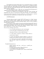
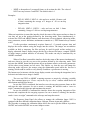
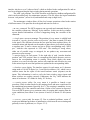
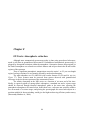
Actually, the Universe sends us light at all wavelengths of the electromagnetic
spectrum. However, most of this light does not reach us at ground level because the
atmosphere blocks out many types of radiation while letting other types through (see Figure 1).
Fortunately for life on Earth, our atmosphere blocks out harmful, high energy radiation like Xrays, gamma rays and most of the ultraviolet rays. It also blocks out most infrared radiation, as
well as very low energy radio waves. On the other hand, our atmosphere lets visible light, most
radio waves, and small wavelength ranges of infrared (IR) light through, allowing astronomers
to study the Universe at these wavelengths.
Most of the IR light coming from the Universe is absorbed by water vapor and carbon dioxide
in the Earth's atmosphere. Only in a few narrow wavelength ranges, infrared light can make it
through (at least partially) to a ground based IR telescopes.
The best view of the IR universe, from ground based telescopes, is at infrared
wavelengths which can pass through the Earth's atmosphere and at which the atmosphere is
dim in the IR. Ground based IR observatories are usually placed near the summit of high, dry
mountains to get the lowest content of water vapor and to stay well above the inversion layer.
Even so, most IR wavelengths are completely absorbed by the atmosphere and never make it to
the ground. The IR windows, where atmospheric transparency is good enough, are mainly at
wavelengths below 5 microns and around 10 micron.
8
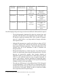
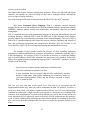
Figure 1 – Atmospheric opacity as function of electromagnetic wavelengths.
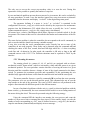
Infrared Windows in the Atmosphere
Wavelength
Range
Band
Sky Transparency
Sky Brightness
1.1 – 1.4 μm
J
high
low at night
1.5 - 1.8 μm
H
high
very low
2.0 - 2.4 μm
K
high
very low
3.0 - 4.0 μm
L
3.0 - 3.5 μm: fair
3.5 - 4.0 μm: high
low
4.6 - 5.0 μm
M
low
high
7.5 - 14.5 μm
N
8 - 9 μm and 10 -12 μm: fair
others: low
very high
17 - 40 μm
17 - 25 μm: Q
28 - 40 μm: Z
very low
very high
very low
low
330 - 370 μm
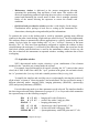
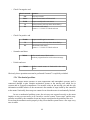
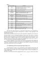
IR is usually divided into 3 spectral regions: near, mid and far-IR. The boundaries
between the near, mid and far-IR regions can vary depending on the type of detector
technology used for gathering IR light 1 .
1
http://coolcosmos.ipac.caltech.edu/
9
SPECTRAL
REGION
WAVELENGTH
RANGE (microns)
TEMPERATURE
RANGE
(degrees Kelvin)
WHAT WE SEE
Near-Infrared
(0.7-1) to 5
740
to
(3,000-5,200)
Cooler red stars
Red giants
Dust is transparent
Mid-Infrared
5 to (25-40)
(92.5-140)
to
740
Planets, comets and
asteroids
Dust warmed by
starlight
Protoplanetary disks
Far-Infrared
(25-40) to (200-350)
(10.6-18.5)
to
(92.5-140)
Emission from cold
dust
Central regions of
galaxies
Very cold molecular
clouds
Near-IR imaging and spectroscopy are much more difficult / different than in optical 2 .
2
•
The sky background is dominated by night sky emission lines, and
especially in the K-bands by the temperature of the atmosphere. The
IR detectors usually get saturated after 10-20 seconds of exposure
time in K, which leads to a very large number of images with rather
short exposure times.
•
Although IR instruments are usually cooled down to about 60-70 K
in order to suppress heat radiation, the telescope and surrounding
dome remain at ambient temperature. Their heat radiation has to be
carefully kept out of the instrument in order to minimize the
background noise.
•
Background subtraction is a critical step since very often the target
sources are significantly fainter than the background noise. IR array
detectors are intrinsically unstable, their response depends on
illumination (hence a mere subtraction of a dark frame as for optical
CCDs it is not sufficient) and can vary on typical timescales of
minutes. This requires a periodic acquisition of background frames
(the so-called sky-frames). Sky frames can be acquired by dithering
techniques and/or by telescope nodding.
•
The read-out of IR detectors is also different from CCDs. Each pixel
is read independently, so for example, there are no blooming effects,
and during an exposure the array can be read several times (multiple
non-destructive read mode, MNDR) in order to reduce the readout
noise (especially useful for spectroscopy).
http://www.ing.iac.es/Astronomy/instruments/liris/liris_obs_tech.html
10
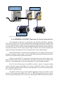
In the recent years, many of the 4-8m class ground-based telescopes have been equipped with
Adaptive Optics (AO) capabilities to improve the overall image quality. An AO system can
potentially remove the effects of the atmospheric turbulence and other optical distortions by
using a suitable wavefront sensor to monitor them and a deformable mirror to compensate for
them.
11
Chapter 2
Overall structure for astronomical software
All wavelength regions are, nowadays, studied by specific instruments and telescopes:
•
Optical astronomy is the part of astronomy that uses optical
components (mirrors, lenses and solid-state detectors) to observe light
from near infrared to near ultraviolet wavelengths. Visible range falls in
the middle of this range.
•
Infrared astronomy deals with the detection and analysis of infrared
radiation (this typically refers to wavelength longer than the detection
limit of silicon solid-state detectors, about 1 μm wavelength).
•
Radio astronomy detects radiation from millimeter to tens of meters
wavelength. The receivers are similar to those used in radio broadcast
transmission but much more sensitive.
•
High-energy astronomy includes X-ray, gamma-ray and extreme UV
astronomy as well as studies of neutrinos and cosmic rays.
The instruments to study each spectral range are very different in concept, kind of arrays and
optic systems but in its general structure the software to manage these devices and to do the
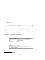
observation is very similar and can be subdivided into 4 main levels (Rossetti, 2008):
•
the low-level software. This level is designed to handle all hardware
related functions and detector controls. It is physically split in two
12
locations: one inside the NICS PC and the other into the embedded
processor (FASTI) located at the focal plane electronics.
•
the middle-level software. This level works like a bridge between the
high-level software and the low-level software managing all commands,
messages and errors.
•
the high-level software. This level is intended to fulfill all astronomyrelated tasks and also to act as an interface between the low-level
software and the astronomer. Hence, it includes several GUI to provide
a full control of all sub-systems.
•
the scientific software. It includes the observing block preparation tools
and the off-line data reduction pipeline.
The goal of the low-level software is to interact directly with the hardware, and to
provide an easy-to-use interface between the electrical devices and the high level software. The
low-level software typically manages directly electronic devices like: array,
temperature/pressure sensors, motors, calibration lamps etc. Usually it is equipped with a
command line interface which allows to communicate using a serial or socket connection to the
external world.
The middle-level software is very useful when we have to communicate with the array.
It is very important to provide a secure and clean communication to prevent damages of these
delicate devices. The middle-level software provides to do that, managing the errors before
their arrival to the low-level software and ensuring a good quality communication checking all
commands sent to the array.
The high-level software provides an interface between the users and the low/middlelevel software. It manages all human errors allowing the interaction with all instruments and
devices. It allows to monitor and have a full control of all sub-systems such as the telemetry,
the calibration lamps status, the motors status and the setting up of all the observational
parameters.
The scientific software is composed by packages of facilities tools dedicated to simplify
the data reduction and the planning of the observations. Usually includes a quick-look software
which ensures a wide displayer for the images visualization comprehending the possibility of:
•
making a field zoom
•
creating a box around the object to do statistics
•
estimating some important parameters like Full Width Half Maximum
(FWHM) and relatives sigma in x and y, the peak of the intensity, the
background value etc...
These criteria ensure a stable, complete and user-friendly GUI; for these reasons the GUI for
NICS at the TNG, has been developed following this structure (see Chapter 4).
13
14
Chapter 3
Graphical User Interface
A Graphical User Interface (GUI) is a type of user interface which allows people to
interact with electronic devices like computers, hand-held devices, household appliances and
office equipment. A GUI offers graphical icons, and visual indicators as opposed to text-based
interfaces. The actions are usually performed through direct manipulation of the graphical
elements. The term came into existence because the first interactive user interfaces to
computers were not graphical; they were text-and-keyboard oriented and usually consisted of
commands you had to remember and computer responses that were infamously brief. The
command interface of the DOS (Disk Operating System) is an example of the typical usercomputer interface before GUI arrived. An intermediate step in user interfaces between the
command line interface and the GUI was the non-graphical menu-based interface, which let
you interact by using a mouse rather than by having to type in keyboard commands. Elements
of a GUI include such things as: windows, pull-down menus, buttons, scroll bars, iconic
images, wizards, mouse pointer etc.
A major advantage of GUI is that they make computer operation more intuitive, and thus easier
to learn and use.
The GUI allows users to take full advantage of the powerful multitasking (the ability for
multiple programs and/or multiple instances of single programs to run simultaneously)
capabilities of modern operating system by allowing such multiple programs and/or instances
to be displayed simultaneously. The result is a large increase in the flexibility of computer and
devices use with a consequent rise in user productivity. The GUI has become much more than a
mere convenience. It has also become the standard in human-devices interaction. Moreover, it
has led to the development of new types of applications and entire new industries.
15
3.1 Why a new NICS GUI
The necessity of a new GUI for NICS is due to the hardware evolution. The hardware
evolution normally leads up to the necessity of a software update in order to fully exploit new
technology. A GUI to properly work, needs to be based on libraries. A library is a collection of
subroutines or classes used to develop software. Libraries contain code and data that provide
services to independent programs.
Some operative systems and libraries may not be compatibles with the oldest softwares.
For this reason, usually, the PC dedicated to an instrument is updated with care to the latest
software versions to avoid the problems due to the incompatibility risks. Year after year the
software/hardware update necessity becomes more and more important until it becomes
essential. The best solution is to develop a new GUI based on the newest software and libraries
to exploit the new hardware resources.
3.2 Tcl/Tk language for GUI developing
Nowadays, there are a lot of different languages for GUI developing; some of the most
used are: Perl, Java, Python, C++, HTML, PHP, IDL and Tcl.
For the new NICS GUI developing I used Tcl for the follow reasons:
•
•
•
•
•
•
•
•
•
All data types can be manipulated as strings, including code.
Everything can be dynamically redefined and overridden.
Everything is a command, including language structures.
Extremely simple syntactic rules.
Event-driven interface to sockets and files. Time-based and user-defined
events are also possible.
Simple exception handling using exception code returned by all command
executions.
All commands defined by Tcl itself generate informative error messages on
incorrect usage.
Readily extensible, via C, C++, Java, and Tcl.
Interpreted language using byte-code for improved speed whilst maintaining
dynamic modifiability.
Tcl stands for Tool Command Language3. Tcl is a scripting language, and an interpreter for
that language that is designed to be easy to embed into the applications. Tcl and its associated
graphical user-interface toolkit, Tk, were designed and crafted by Professor John Ousterhout of
the Berkeley University of California and provides a “virtual machine” that is portable across
UNIX, Windows, and Macintosh environments.
The Tcl interpreter has been ported from UNIX to DOS, Windows, OS/2, NT, and
Macintosh environments. The Tk toolkit has been ported from the X window system to
Windows and Macintosh.
As a scripting language, Tcl is similar to other UNIX shell languages such as the Bourne
3
http://www.tcl.tk/about/index.html
16
Shell (sh), the C Shell (csh), the Korn Shell (ksh), and Perl. Shell programs let you execute
other programs. They provide enough programmability (variables, control flow, and
procedures) to let you build complex scripts that assemble existing programs into a new tool
tailored for your needs.
It is the ability to easily add a Tcl interpreter to your application that sets it apart from other
shells. Tcl fills the role of an extension language that is used to configure and customize
applications.
The Tcl C library has clean interfaces and it is simple to use. The library implements the
basic interpreter and a set of core scripting commands that implement variables, flow control,
and procedures. There is also a set of commands that access operating system services to run
other programs, access the file system, and use network sockets.
There are many Tcl extensions freely available on the Internet. Most extensions include a C
library that provides some new functionality, and a Tcl interface to the library. The script-based
approach to user interface programming has three benefits:
•
Development is fast because of the rapid turnaround: there is no
waiting for long compilations.
•
The Tcl commands provide a higher-level interface than most
standard C library user-interface toolkits. Simple user interfaces
require just a handful of commands to define them.
•
The user interface can be factored out from the rest of your
application. The developer can concentrate on the implementation
of the application core and then fairly painlessly works up a user
interface. The core set of Tk widgets is often sufficient for all your
user interface needs. However, it is also possible to write custom
Tk widgets in C, and again there are many contributed Tk widgets
available on the network.
Moreover, Tcl/Tk is largely used for developing specific astronomical tools and applications
like:
4
5
6
7
8
9
•
DS9 SAOImage4 (HEA Harvard-Smithsonian Center for Astrophysics)
•
Skycat5 (ESO, communication with astronomical archives and catalogs date)
•
Fv6 (NASA, fits viewer)
•
RAC7 (NASA, radio astronomy controller)
•
BOB8 (ESO, manage Observation Blocks at VLT)
•
COBRA9 (Jodrell Bank Observatory).
http://hea-www.harvard.edu/RD/ds9/
http://archive.eso.org/cms/tools-documentation/skycat
http://heasarc.nasa.gov/docs/software/ftools/fv/
http://dsnra.jpl.nasa.gov/development/rac/
http://www.eso.org/sci/facilities/lasilla/sciops/observing/bob.html
http://www.jb.man.ac.uk/research/pulsar/tech03/
17
Chapter 4
TNG and NICS
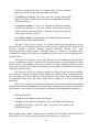
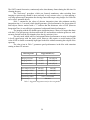
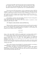
The TNG (Figure 2) is a new concept telescope located in the Roque de Los
Muchachos, La Palma (Canary Islands). To take full advantage of the seeing quality in this site
(Milian M., 1996), the TNG is furnished with an active optical correction system which allows
to minimize the errors due to the mechanical components: micro bend effects, thermal
dilatation etc... The air flux inside the telescope dome is constantly monitored and regulated to
improve the seeing near the incoming optical beam.
The optical design is a Ritchey-Chretien type with two hyperbolic mirrors: the principal
mirror called M1 is concave with a diameter D = 3.6 m and the second one (M2) is a convex
mirror which provides a focus at F/11. The third mirror is plane (M3) and provides two
Nasmyth focus (named A and B). The TNG is provided with an alt-azimuth mount. For this
reason the telescope needs a field derotator for each Nasmyth.
The TNG is equipped with a mechanic derotator which consists in a flange ring with a
diameter D = 1.7 m in which are mounted the scientific instruments. These flange rings can
rotate to 295 degrees in both directions around the elevation axes of the telescope. Each of
those are equipped with an optical pointing system, the auto-guide and a Shack-Hartmann
wavefront sensor (WFS) for the optic active corrections, performed on M1 through 78
actuators.
TNG (Barbieri C., 1989), with its instruments, allows astronomers to investigate optical
and Near-Infrared (NIR) wavelengths. In particular to study the NIR ranges, TNG is equipped
with NICS and in the near future will be equipped also with GIANO (Oliva E., 2006).
18
Figure 2 – The Telescopio Nazionale Galileo.
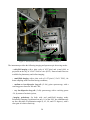
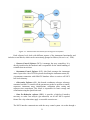
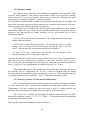
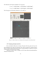
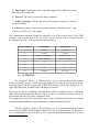
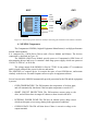
NICS is the TNG infrared (0.9-2.5 µm) multi-mode instrument which is based on a
HgCdTe Hawaii 1024x1024 array. It was designed and built for the TNG by the infrared group
at the Arcetri Observatory in Firenze (Italy) and placed in Nasmyth A as shown in the
following image (Baffa C., 2001).
19
OEM motors
controller
Nics
Fasti
Lakeshore 330
Balzers
DualGauge
Lantronix
Figure 3 – NICS and the electronic devices mounted in Nasmyth A.
The instrument provides the following imaging and spectroscopic observing modes:
wide-field imaging with a plate scale of 0.25''/pixel and a total field, as
projected on the sky, of 4.2'x4.2' field of view (FOV). Narrow-band filters are
available for photometry and in-line imaging;
•
small-field imaging with a plate scale of 0.13''/pixel (2.1'x2.1' FOV), for
better sampling under excellent seeing conditions;
•
medium to low-dispersion long-slit (4' slit) grism spectroscopy with a
resolving power between 300 and 1300;
•
very low-dispersion long-slit (4' slit) spectroscopy with a resolving power
~50, by means of an Amici prism;
•
imaging polarimetry for both wide and small-field imaging mode.
Polarimetry imaging is performed on only 1/4 of the FOV, but simultaneously
on four directions of polarization angle (0, 45, 90, and 135 degrees), with a
clear gain of relative sensitivity;
•
20
spectro-polarimetry with a reduced (25%) slit length, but with four directions
of polarization angle (0, 45, 90, and 135 degrees) measured simultaneously.
•
Three of these modes: low-dispersion, long-slit, spectroscopy and simultaneous angle
polarimetry/spectro-polarimetry are unique to NICS (Baffa C., 2001), and provide, the
possibility to reliably perform these measurements in the infrared.
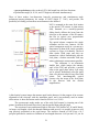
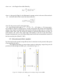
NICS is mounted at the same focal station
as the optical CCD camera. A plane mirror
(M4), mounted on a remotely-operated
sliding bench, deflects the beam from the
telescope to the entrance of the IR camera,
that has its optical axes perpendicular
respect to the telescope beam.
The optical scheme comprises the single
collimator and the two cameras. All the
optical components reside in a vacuum at a
temperature of about 80 K, inside a suitable
cryostat (see Figure 4 for details). The focal
plane masks (field stops and slits) are
mounted on a wheel. Immediately after the
focal plane, a further removable field stop
makes polarimetric measurements possible.
The collimator is an achromatic
doublet lens, which images the entrance
pupil of the TNG and provides a parallel
beam at the pupil plane where Lyot stops
can be placed. Immediately after the pupil
plane, two adjacent wheels carry filters and
grisms. Two interchangeable optical
systems relay the image of the focal plane
on the detector with the desired
magnification.
Figure 4 – Mechanical Layout of NICS cryostat.
A third optical system images the entrance pupil on the detector, for the purpose of an accurate
alignment of the telescope with the instrument pupil, and is not normally used in routine
observations. A short discussion can be found in Gennari et al (1995).
The spectroscopic mode makes use of the wide–field camera by inserting one of the
grisms, located on the second filter wheel, into the parallel beam after the pupil.
The rejection of stray and thermal light is left to the TNG baffles in J, H, and K bands.
At longer wavelengths, where the thermal radiation could prevail, it is possible to insert a cold
stop precisely positioned at the pupil image. The sensitive element of NICS has a 18.5
μm/pixel pitch and is sensitive to radiation at wavelengths between ~0.90 μm and ~2.5 μm. Its
21
performance in term of dark current, efficiency, and read noise, is comparable or better than the
256 × 256 NICMOS 3 (e.g. Lisi et al.,1996). The electronic noise is dominated by the detector
and by the first cold amplifier and is ~25 e− , if a suitable number of detector resets (more than
32) is performed at each integration.
4.1 NICS in imaging mode
The LF offers a 4.2'x 4.2' FOV and a pixel scale of 0.25'' /pixel. The LF images are, on
the other way, characterized by a significant pin-cushion distortion which is intrinsic to the
optics design and amounts to 1% at the edges and 3% at the array corners. This effect is
wavelength independent and can be accurately modeled and corrected for during the image
reduction.
The small field camera (SF), with its 2.1'x2.1' FOV and a pixel scale of 0.13'' /pixel, is
primarily intended for imaging programs, requiring a fine sampling of the point spread
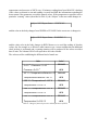
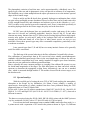
function. LF and SF main characteristics are shown in Table 1.
Camera
Image scale
Field of view
LF
0.25"/pix
4.2' x 4.2'
SF
0.13"/pix
2.2' x 2.2'
LF+Adopt
0.08"/pix
1.4' x 1.4'
SF+Adopt
0.04"/pix
0.7' x 0.7'
Table 1 - Main characteristics of LF and SF camera.
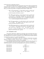
The instrument is equipped with a number of broad and narrow band filters which are listed in
Table 2.
Filter
Center wl (µm)
FWHM (µm)
K
2.20
0.34
K'
2.12
0.35
H
1.63
0.30
J
1.27
0.30
Js
1.25
0.16
1mic
1.02
0.13
Kcont
2.275
0.039
Brgamma
2.169
0.035
H2
2.122
0.032
FeII
1.644
0.027
Hcont
1.570
0.023
CH4s
1.60
0.12
CH4l
1.68
0.12
SW
Cut-off 1.75
Cut-off 1.75
Table 2 - Filters characteristics.
22
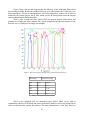
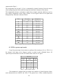
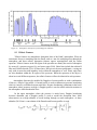
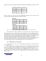
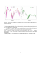
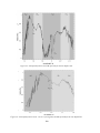
Figure 5 shows the spectral response and the efficiency of the wide band filters which
are presently available. Besides the standard filters for J, H, and K bands, NICS offers the 1 μm
filter centered at 1.030 μm in correspondence with a fair atmospheric window, the Jn filter as
defined by the Gemini project, the K' filter which cuts the K band portion where the thermal
emission dominates the background flux.
There is also a band pass filter (labeled SW) for general purpose observations and
pointing and a high–pass filter (labeled LW) which, along with the spectral response of the
detector, acts as a band pass for longer wavelengths.
Figure 5: Spectral response and efficiency of NICS wide-band filters.
Wavelength
Attenuation (mag)
(µm)
gray5
gray10
1.03
4.8
~9.5
1.25
5.1
~10.0
1.65
5.5
~10.5
2.15
5.7
~11
Table 3 – Attenuators characteristics.
NICS is also equipped with two attenuators (gray filters) which can be used in
combination with any of the broad and narrow band filters whenever observing bright objects
which would otherwise saturate the detector. The main characteristics of the gray filters are
23
summarized in Table 3.
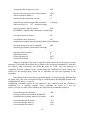
The background flux beyond 2.15 µm is dominated by thermal emission from the mirrors
which strongly depends on the ambient temperature and on the cleanness of the mirrors.
The background at shorter wavelengths is mainly due to airglow emission which may vary by
up to about a magnitude on time scales of hours. A list of typical values of zero points and
background sky emission is shown in Table 4.
Filter
Zero point
(mag per 1 ADU/sec)
Background
(mag/sq-arcsec)
K
21.8
12.5-13.0
K'
21.9
13.1-13.6
H
22.3
13.4-14.7
J
22.1
15.0-16.0
Js
22.1
15.0-16.0
1mic
22.5
16.0-17.0
Kcont
18.8
12.5-13.0
Brgamma
18.8
13.0-13.5
H2
18.8
13.5-14.0
FeII
19.2
13.4-14.7
Hcont
19.1
13.6-14.9
SW
~23
13.5-14.5
Table 4 - Typical values of zero points and background sky emission.
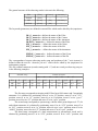
4.2 NICS in spectroscopic modes
Long slit spectroscopic observations are performed by inserting a slit (see Table 5) at
the entrance focal plane and a disperser (grism or prism) in the collimated beam. All
spectroscopic modes make use of the LF camera with a scale of 0.25"/pixel.
NICS slits
Name
Width
Length
0.5
0.5" = 2 pix
4'
0.75
0.75" = 3 pix
4'
1.0
1.0" = 4 pix
4'
1.5
1.5" = 6 pix
4'
2.0
2.0" = 8 pix
4'
Table 5 – Slits available in NICS.
The instrument is equipped with one prism and a number of grism dispersers whose
main characteristics are listed in the Table 6. The grisms have a fairly constant dispersion
24
(Å/pix) throughout the spectrum and, therefore, their resolving power increases going towards
the red. The Amici prism, on the contrary, delivers a spectrum with a quasi-constant resolving
power and its dispersion varies by more than a factor of 3 over its spectral range. All the low
resolution dispersers can be used in combination with the gray filters to take spectra of very
bright objects which would otherwise saturate the array.
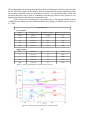
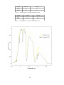
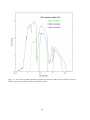
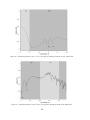
Figure 6 shows the resolving power (associated to the 1'' slit) and the efficiency of the
available grisms which are resin–replicated Milton-Roy gratings on IRGn6 prisms (Vitali et
al., 2000).
NICS dispersers
Low resolution
Name
wl-range (µm)
dispersion (Å/pix)
Res.power with 1" slit
Amici
0.8-2.5
30-100
50
IJ
0.9-1.45
5.5
500
JH
1.15-1.75
6.6
500
JK'
1.15-2.23
11.6
350
HK
1.40-2.50
11.2
500
0.96-1.09
2.0
1250
Js
1.17-1.33
2.5
1200
J
1.12-1.40
2.5
1200
H
1.48-1.78
3.5
1150
High resolution
1mic
KB
1.95-2.34
4.3
Table 6 – NICS grism dispensers and main characteristics.
Figure 6 – Resolving power and efficiency of NICS grisms.
25
1250
4.3 NICS detector
The detector is a Rockwell 1024x1024 HgCdTe Hawaii array which, alike other devices
used in various astronomical instruments, has some peculiar characteristics.
Data acquisition and control system are based on the controller developed by the CCD
Working Group of TNG, suitably modified to adapt it to the architecture of infrared arrays
(Baffa, C., 2001). The controller is based on a set of Transputer processors, which are
responsible for handling data and sending commands, and on a DSP Motorola 56001, which
generates the synchronized clock pattern needed for accessing and reading the array
multiplexer.
The analog signal read on each pixel of the four quadrants is buffered by four FET
amplifiers located on the same board that hosts the detector. After that stage, there is a set of
four 16-bit A/D converters, which convert the pixel intensity of the four quadrants in parallel.
The parallel outputs from the converters are translated to the Transputer serial protocol using a
dedicated programmable logic chip from Xilinx.
The Transputer stage sends the digital data to a Linux PC by means of a fiber link
which exploits the fast serial connection capability built into each Transputer. The controller
takes care of telemetry and stepper motors by means of dedicated RS–232 serial ports.
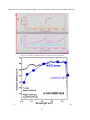
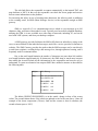
The array multiplexer has a stubborn attitude to remember whatever strong signal was
recorded in the previous frame(s). This ghost image will also persist in the subsequent frames
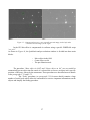
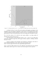
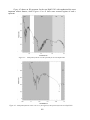
with intensity slowly fading down to below the noise level (see Figure 7).
Figure 7 - Evolution of the level of persistency signal (ghost) after a strongly
saturated frame. The level of persistency has decreased about a
factor of 3 after the new acquisition electronics (FASTI- NICS).
Contrary to standard CCD devices, the "bias" of this detector is not uniform over the
array, but has a distinct horizontal pattern with pronounced maximum at rows Y=1 and Y=513.
26
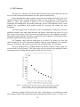
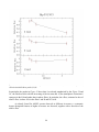
Moreover its level is not constant along a row but increases with X (see for example Figure 8).
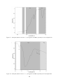
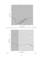
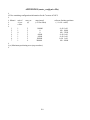
Figure 8 – NICS array quantum efficiency function of the wavelength.
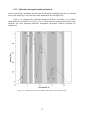
Figure 9 - A typical 60s dark frame with cuts along the two axes shows the NICS detector bias.
27
The amplitude of the peaks and their slopes are not constant but strongly vary with the
level of the signal. In dark exposures, the pattern is characterized by a prominent maximum
with quite gentle slopes, while at higher levels of illumination, the peaks become progressively
narrower. This effect could produce annoying features when subtracting images/spectra taken
under variable sky conditions.
The values displayed in Figure 9 (blue dots) were determined from measurements of
standard stars both in imaging and low resolution spectroscopy (prism).
The data were corrected for the transmission of the optics, filters and prism and
normalized to the value at 2.2 micron given in the typical efficiency curve (black triangles).
Evident and somewhat unexpected is the quite rapid decrease of efficiency below 1.4 microns
which translates into a significant loss of sensitivity in the J and 1micron bands.
4.4 NICS electronics
The infrared detector control is named FASTI. FASTI meant to be a "light" electronic
system, which is modular, flexible, extendible, and avoids obsolescence as much as possible.
The design does not constrain the downhill controlling computer: FASTI is seen as a peripheral
through a network connection.
FASTI contains a central controller for start-up, general housekeeping, global control of
operations (start integrations for example), data collection, formatting and buffering, or for data
pre-processing when needed. That is realized with a disk-less embedded computer, using an
Intel or Alpha family CPU and a number of commercial boards.
There are many advantages in this choice:
•
it is very flexible and its behavior can be easily changed
•
it is fast and capable of substantial data pre-processing
•
it has plenty of built-in or easily available interfaces
•
it is much cheaper compared to alternate solutions based on
custom interface adapters
•
it is seen by the instrument controller computer as a socket in a
standard (or fast) Ethernet connection, giving no constraints on it
•
it is scalable and can be replaced with similar models (hopefully
more powerful) without big modifications to the existing
software
The global characteristics are:
•
•
•
•
standard interfaces and bus: a serial port, a parallel port,
Ethernet, PCI bus
no moving part (such as hard or floppy disk drivers)
very fast parallel interface (described later)
it can be used as an embedded system, with no external human
interaction
28
The FASTI control electronics, continuously takes short dummy frames during the idle time for
cleaning the array.
The "clear-array" procedure, which was formerly mandatory when switching from
imaging to spectroscopy, should be now used only in very extreme cases, e.g. when starting a
very long spectroscopic integration after having centered the target using images of a field with
one or more saturated objects.
Table 7 summarizes the values of detector integration times (the minimum on-chip
integration time is 3 seconds) which should guarantee good performances for observations of
faint objects. Entries marked with a "*" indicate that the maximum value of DIT (Detector
Integration Time) is not sufficient to guarantee background-limited performances.
The imaging with the SF should require integration times a factor of 4 longer than those
with the LF. In spectroscopy, the data taken with low and medium resolution grisms are readout noise limited at all the wavelengths where the sky emission is low.
The only mode which achieves background limited performances at most wavelengths
is low-R spectroscopy with the Amici prism. However, this requires a careful tuning of the
value of DIT to obtain a reasonably high signal in the blue without saturating the red part of the
spectrum.
The value given in Table 7 guarantees good performances in the blue with saturation
starting at about 2.4 microns.
Observing mode
Suggested DIT (sec)
Imaging J/Js/1mic
60 (LF)
240 (SF/pol)
Imaging H/K'/K
25 (LF)
100 (SF/pol)
Ima narrow band
150 (LF)
600 (SF/pol)
Ima+AdOpt J/Js/1mic
600 (LF)
600*(SF)
Ima+AdOpt H/K'/K
240 (LF)
600*(SF)
Ima+AdOpt N.B.
600*(LF)
600*(SF)
Spectroscopy Amici
120 x (1"/slit-width)
Spectroscopy
600-900*
Table 7- Suggested integrations time for observing modes.
29
Chapter 5
The NICS interface
In its general structure the NICS software system can be subdivided into 4 main levels
as already described in Chapter 2 and here summarized:
•
the low-level software. This level is designed to handle all hardware related
functions and detector controls. It is physically split in two locations: one
inside the NICS PC and the other into the embedded processor located at the
focal plane electronics.
•
the middle-level software. This level works like a bridge between the high-level
software and the low-level software managing all commands, messages and
errors.
•
the high-level software. This level is intended to fulfill all astronomy-related
tasks and also to act as an interface between the low-level software and the
astronomer. Hence, it includes several GUIs to provide a full control of all subsystems.
•
the scientific software. It includes the pre-reduction facilities and some useful
tools for the observations.
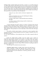
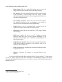
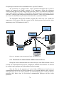
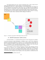
Figure 10 shows the main architecture of the NICS Control Software.
30
Figure 10 - Main architecture blocks for the high-level software.
Each software level deals with different aspects of the instrument functionality and
includes several blocks, which can be conveniently grouped as follows (Rossetti et al., 2008):
• Detector Control Software (DCS): it manages the array controllers. It is
directly interfaced to the hardware and is responsible for the initial handling of
scientific data in real time.
• Instrument Control Software (ICS): this block manages the instrument
status. It provides a list of FITS keywords describing the instrument status (IS).
A permanent connection with ORACLE database allows to retrieve all NICS
low-level telemetry.
• Observation Software (OS): this branch coordinates telescope telemetry
command variables. It controls all the parameters needed to perform scientific
exposures: instrument setup, initializations, calibration units, setting and
exposure time count-down. This block is responsible for frame storage and
visualization using the Quick-look task.
• Data Pre-Reduction software (DRS): it provides a high-level interface
necessary to make fast analysis (pre-reduction) on all the NICS acquired
frames like a sky subtraction, apply a cross-talk correction etc...
The NICS interface communicates with the array control system via socket through a
31
dedicated “bridge” program running on the same PC (see Chapter. 6.1). The DCS consists of
two different parts: the first resides inside the PC-Linux and the second runs on the embedded
processor at the focal plane electronics and has direct access to the hardware. The two branches
are interfaced by means of a standard Ethernet connection, on which data and commands are
sent to Unix-like sockets. The software portion inside the embedded processor manages the
data flow controls and can handle special observing modes such as multiple starts and stops.
More specifically, it can perform any of the following tasks:
•
setting the array read-out mode and detector integration time
(DIT)
•
starting an integration and, at its end, transferring the resulting
frame to the instrument workstation
•
averaging a NDIT number of individual DITs before transferring
the image
•
executing a sequence of dummy images (useful to clean the array
from persistence effects)
A typical observation with NICS consists of a mosaic of exposures taken with the
telescope pointing at different positions (coordinates) in the sky. Informations on the mosaic
positions are saved in the header fits files where the images are stored (see Chapter 5.1.5).
Each exposure produces and writes on disks a number of frames characterized by the DIT,
NDIT parameters. These parameters are saved in the header of the fits files where the images
are stored.
The interface includes separate buttons to start/stop the various acquisition modes
foreseen by the system. A running acquisition can always be stopped or aborted by the user as
described in Chapter 5.1.
The last acquired integration is always displayed using a Ds9 window integrated within the
interface.
Besides the standard buttons available in the Ds9 window (some of which are
deactivated by the program), the interface also includes a few buttons which can be used to
modify the display and to perform a few analysis on the image. The latter includes
measurements of the FWHM of the stellar profile, the possibility of selecting an object and
move it to a certain position of the field by offsetting the telescope (see Chapter 5.3.1) and the
procedure to compute and execute the telescope offsets necessary for centering the object in
the slit (see Chapter 5.3.2).
The Observing GUI is divided in three main windows:
•
Acquisition window manages everything which concerns the single frames or
mosaics acquisitions. It allows the observing mode selection and setting
acquisitions parameters like: DIT, NDIT, NINT, calibration lamps etc.. Also
provides detailed and useful informations on telemetry parameters, telescope
and NICS status.
32
•
Maintenance window is dedicated to the motors management allowing
operations like positioning, Stop and Reset of each motor. This window also
checks all engineering parameters allowing the users to have a complete motors
control and monitoring the overall status of them. Also it manages potential
blocks of the motors allowing the superuser to restore the normal work
conditions.
•
Quick-look and pre-reduction window provides a wide display for the images
visualizations and a package of tools acts to: setting up the instruments for
observations, showing the seeing and radial profiles informations.
To optimize the space on the desktop and to avoid its saturation, opening many different
windows in the same virtual desktop, a light software called Devilspie10 has been implemented.
This software allows to automatically redirect applications to a specific virtual desktop. At the
startup, Devilspie looks for scripts ending with ".ds" in a ".devilspie" directory in the home
directory. The “.ds” files have been opportunely configured to organize the windows in three
virtual desktops: the workspace 1 is reserved for the Observing window, the second one for the
Quick-look window and the third one is used for the maintenance window. In this way, the
user, has at hand all the instruments in separated windows avoiding confusions due to their
overlapping.
5.1 Acquisition window
NICS observational modes require selecting a given combination of the elements
mounted on the 7 movable axis existing inside the cryostat.
For example, large field imaging in K requires selecting: the “LF” camera in the camera
wheel, the K filter in the filter wheel, the ”open” position in the grism, slit and mask wheels,
the “in” position in the Lyot-stop slide and a suitable position of the focusing slide.
To simplify the interface and avoid the user to work manually selecting the position of
all the wheels, a system of ”observing modes” has been defined. The user can choose among 4
different observing modes: imaging (IMA), imaging polarimetry (IMAPOL), spectroscopy
(SPE) and spectro-polarimetry (SPEPOL).
For each observing mode up to three parameters can be selected. The interfaces handles
the observing modes and relative parameters as groups of 2, 3 or 4 keywords which summarize
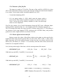
the requested setup as in the following examples :
IMA
K LF G0
IMA
K LF G5
IMAPOL J
SPE
IJ 1.0 G0
SPE
IJ 1.0 G10
SPEPOL HK 1.5
:
:
:
:
:
:
Imaging in K with LF objective
as above but with a 5-mag gray filter
Imaging polarimetry in J
Spectroscopy with IJ grism and 1.0'' slit
as above but with 10-mag gray filter
Spectropolarimetry with a HK grism and 1.5'' slit
10 http://burtonini.com/blog/computers/devilspie
33
The general structure of the observing modes is shown in the following:
IMA
[Filter]
[Camera]
[Attenuator]
IMAPOL
[Filter]
---
---
SPE
[Grism]
[Slit]
[Attenuator]
SPEPOL
[Grism]
[Slit]
---
The keywords (parameters) are defined in external files which can be edited by the (super)user:
IMA_1_menu.nics : defines the names of the Filter
IMA_2_menu.nics : defines the names of the Camera
IMA_3_menu.nics : defines the names of the Attenuator
IMAPOL_1 menu.nics : defines the names of the Filter
SPE_1_menu.nics : defines the names of the Grism
SPE_2_menu.nics : defines the names of the Slit
SPE_3_menu.nics : defines the names of the Attenuator
SPEPOL_1_menu.nics : defines the names of the Grism
SPEPOL_2_menu.nics : defines the names of the Slit
The correspondence between observing mode setup and positions of the 7 axis (motors) is
defined within the text file “obsmodes_tab.nics” which can be edited by the (super)user for
maintenance purposes.
This file contains comments (records starting with “#”) and one record per observing setup as
in the following examples :
Obsmode.setup
Position of motors
#1
#2
#3
#4
#5
#6
#7
IMA
H
LF
G5
LF
LF1
in
H
gray5
LF
open
SPE
Amici
0.75
G0
LFS
LF1
in
open
Amici
0.75
open
SPE
Dark
1.00
G0
LFS
any
any
any
close
any
any
The first setup corresponds to imaging with H filter, large field camera and 5-magnitude
attenuator. It is obtained by positioning motor#1 at its LF position, motor#2 at its “LF1”
position, motor#3 at its “in” position, motor#4 at its H position, motor#5 at its “gray5”
position, motor#6 at its “LF” position and motor#7 at its “open” position.
The second setup corresponds to spectroscopy with the Amici-prism disperser, 0.75'' slit
and without attenuator, it is obtained by positioning motor#1 at its “LFS” position, motor#2 at
its “LF1” position, motor#3 at its “in” position, motor#4 at its “open” position, motor#5 at its
“AMICI” position, motor#6 at its 0.75'' position and motor#7 at its “open” position.
The third setup corresponds to a dark measurement in spectroscopic mode and is
obtained by positioning motor#1 at its “LFS” position, motor#5 at its “close” position, and
34
leaving the other motors at the current position (keyword any).
The translation between motor position keywords and physical positions (i.e. encoder steps) is
performed using the information contained in the text files “motor1_pos.nics” through
“motor7_pos.nics” which can be edited by the (super)user for maintenance purposes. The
structure of these files is described in the header and comment lines of each file.
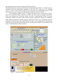
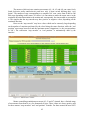
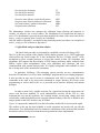
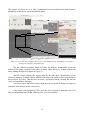
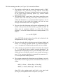
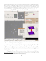
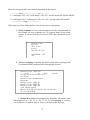
The acquisition window (Figure 11) allows the users to have a full control of NICS,
show the overall NICS status, telemetry variables and allows users to manage acquisitions.
Users can introduce the observing setting, can start a single/multiple frame or mosaic
acquisition, monitor the motors status and all telemetry parameters, manage the calibration
lamps and the connection with the telescope (obviously if there is no connection with the
telescope the mosaic tools will be disabled). This window is also equipped with a detailed log
window act to provide an historical observations log and giving moreover, the possibility to the
users, to manually add personal comments.
Figure 11 – Acquisition window.
35
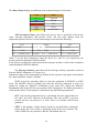
The Motors Status display uses different color to show the status of each motor:
Color
Status
Green
In position
Blue
Moving
Red
Error
Grey
Not set
Yellow
Not in position
NICS Instrument Status panel allows the users to have a quick-look of the dewar
status, showing temperatures and pressure values. The text color changes when the
temperature/pressure increase over the normal ranges as shown in the following:
Green
Orange
(K)
Red
Tn <= 80 (K)
80 < Tn < 100
Tn >= 100 (K)
TArray <= 87 (K)
87 < TArray < 95 (K)
TArray >= 95 (K)
PArray <= 0.000005 (mbar)
0.000005 < PArray < 0.0005 (mbar)
PArray >= 0.0005 (mbar)
Where Tn are the three temperature along the dewar, PArray and Tarray are respectively, the
pressure and the temperatures inside the dewar.
It also allows to manage the connection with the telescope and have a look on the connection
status through the ORACLE database.
The Telescope telemetry panel shows all the telescope telemetry parameters retrieved
from the ORACLE database (see Chapter 6.6).
Instrument setups for the observations are defined in the exposure setup panel which include
the “Start acquisition” and the “FreeRun”.
START Acquisition procedure allows to start the acquisition in MOSAIC or NINT
mode. The MOSAIC mode is available only when the telescope connection is active. It's
granted by setting the MOSAIC checkbutton in the status ON. Setting the MOSAIC
checkbutton in the status OFF the user performs NINT integrations. The frames generated are
saved into the archive. Each exposure is characterized by the following parameters:
•
DIT, is the on-chip integration time or, equivalently, the time elapsed between
the “start” and “end” read-outs of the detector. The value of DIT is given in
seconds and can vary between 3 to 9999. There is no default value for this
parameter.
•
NDIT, is the number of single frames which are averaged before writing the
image on the disk. The average is performed by the lower level software. The
value of NDIT can vary between 1 and 100. The default value is 1.
36
•
NINT, is the number of (averaged) frames to be written the disk. The value of
NINT can vary between 1 and 9999. The default value is 1.
Examples:
•
DIT=20, NDIT=2, NINT=4 : take and save on disk 4 frames each
of them containing the average of 2 images of ~20 sec on-chip
integration time.
•
DIT=900, NDIT=1, NINT=1 : take and save on disk 1 frame
containing 1 image of ~900 sec on-chip integration time.
When an Acquisition is started the interface check the status of the motors and moves them in
case they are not at the position defined by the observing mode. Then, simultaneously, it
activates the STOP and ABORT buttons, and deactivates all set-up buttons (observing mode,
array parameters, mosaic definition, maintenance controls etc.). EXIT button always remains
active.
FreeRun procedure continuously acquires frames of ~3 seconds exposure time and
displays the results without saving the images into the archive. The images are nevertheless
available on disk as temporary fits files and may be used for quick on-line analysis (e.g.
display subtracted frames, display images divided by reference-flat frames, compute FWHM
of stellar images, perform statistics of sub-areas). This mode can only be terminated by an
ABORT command.
When a Free-Run is started the interface checks the status of the motors simultaneously
and move them in case they are not at the position defined by the observing mode. Then
activates the ABORT button and deactivate the set-up buttons relative to the array parameters.
All the other set-up buttons are left active. This implies e.g. that the user can change the
observing mode and move the motors using the maintenance panel while the free-run is
running, which could be useful to verify directly if and how a given motor is moving.
The buttons used to interact with the image display remain active during the integration, but is
be deactivated when a new image is loaded.
The user can STOP or ABORT a running exposure or mosaic by selecting a suitable
key. This command pops-up a “Please confirm the stop (or abort)” window which blocks all
other buttons until the user answer.
In case the STOP is confirmed, the interface saves the on-going exposure frame on disk
and stops the other exposures. In case a mosaic is running, the interface sends a “move to
origin” command to the telescope and terminates the mosaic.
In case the ABORT is confirmed the interface aborts the on-going integration of the
detector and completes the the on-going exposure. In case a mosaic is running, the interface
sends a “move to origin” command to the telescope and stops the mosaic.
The Exposure Setup Panel also allows to manage the calibration lamps. NICS is
equipped with three different calibration lamps: Halogen, Xenon, Argon and a diffusor.
The procedure to manage the calibration lamps allows the user to put the diffusor in position
ON/OFF and switch ON/OFF one or more lamps at a time.
37
The connection between the GUI and the lamps is guaranteed by the port number 5 on the
Lantronix. Using this connection the following list of commands allows to manage the
calibration lamps.
Command
Description
#5 / #6
Halogen ON / OFF
#7 / #8
Argon ON / OFF
#9 / #0
Xenon ON / OFF
#r
read all lamps status
#a
put diffusor in ON/OFF state
When the GUI is starting up, an “#r” command is sent to the lamps and their actual status is
shown into the GUI.
The user must wait approximately 20 seconds, while the diffusor is positioning. During this
time the acquisition buttons are disabled but the user can continue working on the current or
latest image.
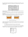
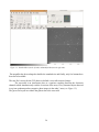
During the diffusor positioning the label “Dif” (Figure 12) is shown in blue color to notify that
diffusor is moving. The color become light green when the diffusor is in “close” position.
Figure 12 - All lamps OFF and the diffusor in Close position (left)
Halogen and Xeno lamps ON (right).
Finally, the GUI shutdown procedure checks the status of the lamps before close the GUI and
notifies, when necessary, if some lamps are ON or if the diffusor is in “open” position allowing
the user to switch OFF.
5.1.1 Defining and performing the telescope movements (mosaic)
A typical IR observations consist of several frames taken with the telescope pointing at
different positions. The instructions on how the telescope should be moved are contained in the
“mosaic files”. They are simple text files (extension .txt mandatory) structured as follows:
[MODE]
X_offset1
X_offset2
X_offset3
X_offset4
X_offset5
....
Y_offset1
Y_offset2
Y_offset3
Y_offset4
Y_offset5
38
The header MODE is optional and specifies how the offsets must be interpreted. Four modes
are feasible:
•
REL2SOURCE_AD: offsets are in arcsec. The first column contains the RA
offset and the second the Declination offsets. The origin (0,0) is the
position of the telescope before starting the mosaic. Offsets are absolute
with respect to this position. This is the default mode. A mosaic without an
header will be interpreted and executed in this way.
•
REL2LAST_AD: also in this case units are arcsec and the columns contain
RA and Dec offsets, but now they are relative to the previous mosaic
position.
•
REL2SOURCE_XY: offsets are in pixels for the LF camera and are defined
along rows (X) and columns (Y) of the array. They are absolute offsets with
respect to the origin (0,0), i.e. the position of the telescope before starting
the mosaic.
•
REL2LAST_XY: the same as REL2SOURCE_XY except that the offsets are
relative to the last mosaic position.
The GUI executes the mosaic command according to the following steps:
1. Reads the mosaic file, determines the offsets and stores the offsets values
2. Moves the telescope to the first mosaic position and waits for telescope settling.
Obviously, this operation is skipped in case the offset amplitudes are both = 0.
3. Acquires frame
4. Moves telescope to next mosaic position and waits for telescope setting
5. Repeats steps 3-4 until the mosaic ends
6. Moves to the origin, i.e. moves the telescope back to the original position of the
mosaic and waits for telescope settling before reactivating the START button.
In case of a STOP or ABORT command the GUI sends the telescope directly to the step 6.
5.1.2 Offsetting the telescope
The interface can move the telescope sending to the tracking the command GDOFFS in the
following format:
GDOFFS dAR dDEC
39
This command is issued to the telescope tracking system through the WSS-bridge (see Chapter
6.5). The parameters dAR and dDEC are the α and δ offsets, in arcsec, to give to the telescope.
Everytime this command is used, the interface must wait for the telescope to settle: first
of all the time necessary for the tracking system to accept the command (about 4 seconds), thus
periodically (every second), check the value of the telemetry variable TRKOK.
The telescope is settled when TRKOK=1. During this waiting the interface blocks the
image acquisition, but allows other operations, e.g. handling of the display etc.
In case the waiting lasts more than 30 seconds (parameter to be stored and read from the
configuration file overall_config.nics) the interface times-out produces an error message. If a
mosaic is running the interface suspends the mosaic leaving the telescope in the current
position and informs the user of the amplitude of the α, δ offsets which must be (manually)
applied to return to the origin position of the mosaic.
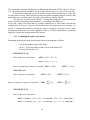
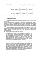
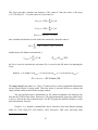
5.1.3 Computing the offsets of a mosaic
Depending on the mosaic mode the telescope offsets are determined as follows:
–
–
–
•
Let θp be the position angle of the frame
Let X(i) , Y(i) be the entries of the i-th line of the mosaic file
Let X(0)=0.0 and Y(0)=0.0
REL2SOURCE_AD
Move to the next i-th position:
dARi= X i− X i−1
dDEC i=Y i−Y i−1
Move to origin from current m-th position: dAR=−X m
•
dDEC=−Y m
REL2LAST_AD
Move to the next i-th position:
dARi= X i
m
Move to origin from current m-th position:
;
dAR=−∑ X j ;
J=1
•
;
dDEC i=Y i
m
dDEC=−∑ Y j
J =1
REL2SOURCE_XY
Move to the next i-th position:
dARi=Scale∗{−[ X i−X i−1]∗cos θp[Y i−Y i−1∗sin θp]}
dDEC i=Scale∗{ [ X i− X i−1]∗sin θp−[Y i−Y i−1∗cos θp] }
40
Move to origin from current m-th position:
dAR=Scale∗[ X mcos θP −Y m sinθ P ]
dDEC=Scale∗[−X msin θP −Y m cosθ P ]
•
REL2LAST_XY
Move to the next i-th position:
dAR=Scale∗[−X i cosθ P Y i sinθ P ]
dDEC=Scale∗[ X isin θP Y icos θP ]
Move to origin from current m-th position:
{[∑ ]
{[ ∑ ]
m
dAR=Scale∗
J=1
[∑
[∑
m
X j cosθ P −
m
dDEC=Scale∗ −
J=1
J=1
Y j sinθ P
m
X j sinθ P −
J=1
]}
]}
Y j cosθ P
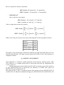
Where Scale is the pixel scale (in arcsec/pix) which depends on observing mode as follows :
IMA-LF
0.25
SPE/POL
0.25
IMA-SF
0.13
IMA-LF-AdOpt
0.086
IMA-SF-AdOpt
0.043
The angle θp is the position angle of the frame, defined as the angle between the detector Y-axis
and the North direction. The angle increases going from North to East. This parameter is
computed as follows:
θp = RPAOFF +NICS_DEROFF
where RPAOFF is a telemetry variable generated by the telescope tracking system, while
NICS_DEROFF is a constant which must be stored and read from the configuration file
overall_config.nics.
During a mosaic the values of DEL_RA, DEL_DEC are shown in green if the mosaic is
of type REL2SOURCE_AD or REL2LAST_AD, otherwise in default color (gray) for
REL2SOURCE_XY or REL2LAST_XY.
The values of DEL_X, DEL_Y are shown in green if the mosaic is of type REL2SOURCE_XY
or REL2LAST_XY, otherwise in default color (gray) for REL2SOURCE_AD or REL2LAST_AD.
41
5.1.4 Structure of the fits files
The images are stored in I*2 fits files. The name of the each file is XXXZiiii.fts, where
XXX is the session name which is create by the telescope tracking and read from the database.
It is a unique 3 letter counter which is normally updated every 24 hr.
•
Z is the label identifying NICS
•
iiii is an integer number (1...9999) which counts the images within a
given session. This counter is updated everytime a new frame is stored. Its
value is saved (also in the telemetry database) to make sure that image
names are never duplicated
Fits files also contain a lot of useful informations about the NICS state, calibration lamps,
motors positions, acquisition time, etc... (an examples of fits file is shown in Appendix A).
The GUI manages the header fits using a specific Tcl library named fitsTcl 2.2.This library is
an extension to the script language Tcl/Tk, which uses the CFITSIO library and provides
general users with a simple interface to read/write FITS file.
5.1.5 Mosaic offsets in the header fits
During a mosaic the values of the offsets, relative to the origin, are also stored in the
header file of the image in the keywords DEL_RA, DEL_DEC, DEL_X, DEL_Y. These values
differ from that sent to the tracking because in that case they are always referred at the
REL2LAST_AD mosaic (see Chapter 5.2.3 for details), while the offset values stored in the
header fits are computed as follows.
Let θp be the position angle of the frame, m be the current position of the mosaic.
•
REL2SOURCE_AD
DEL_RA= X m
;
DEL_DEC= Y m
While the keywords DEL_X and DEL_Y are not saved.
m
•
REL2LAST_AD
DEL_RA=
∑ X j
m
; DEL_DEC=
J=1
∑ Y j
J=1
While the keywords DEL_X and DEL_Y are not saved.
•
REL2SOURCE_XY
DEL_X =
X m
;
DEL_Y= Y m
dAR=Scale∗[−X mcos θP Y msinθ P ]
dDEC=Scale∗[ X msinθ P Y mcos θP ]
42
m
•
REL2LAST_XY:
DEL_X=
m
∑ X j
; DEL_Y=
J=1
{[
DEL_RA Scale∗ −
[∑
{[∑ ]
[∑
∑ X j cosθ P
J=1
m
DEL_DEC=
J=1
]
m
Scale∗
J=1
X j sin θP
∑ Y j
m
J=1
Y jsinθ P
]}
m
J =1
Y jcos θP
]}
Where Scale is the pixel scale (in arcsec/pix) which depends on the observing mode.
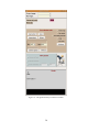
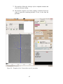
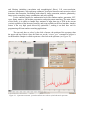
5.2 Maintenance window
The maintenance window is the interface which allows the control of the NICS motors
(see Figure 13).
The NICS instrument includes 7 axis driven by stepper motors. Each of the stepper motors is
controlled by a OEM300 Power Module (Chapter 6.3) which, among other operations, keeps
track of all the movements performed (steps) and updates a "step-encoder" value which, in
practice corresponds, to the absolute position of the axis, unless some mechanical problem
occurs.
The controller holds the value of the step-encoder only as long as it is powered, i.e. the
information is lost when the system is switched off. Consequently, a "reset" operation is needed
whenever the system is turned-off and on and it is also useful to check and correct for
mechanical problems.
The 7 axis/movements perform the following operations:
•
Motor #1 rotates the "cameras wheel" which houses 3 cameras (LF, SF,
PR) and one "close" position. The step-encoders corresponding to the
cameras positions are listed in the text file motor1_pos.nics which can be
edited for maintenance purposes. The wheel can rotate freely (no
mechanical blocks) and has one home-switch used to define the zeroposition. A complete 360˚ turn requires about 100,000 motor steps, the exact
value is stored in the configuration file motors_config.nics.
•
Motor #2 drives the "focus slide" which moves the array detector
perpendicularly to the optical axis. The step-encoders corresponding to the
optimal focus positions in the various observing modes are listed in the text
file motor2_pos.nics which can be edited for maintenance purposes. The
slide has two limit-switches, limiting the movement from 0 to about +9000
steps. Besides these hardware limits, the interface also foresees “software
limits” which are defined in the configuration file motors_config.nics and
are used to avoid approaching the limit switches during normal operations.
A home switch is also present but, in practice, is not used.
43
•
Motor #3 drives the "pupil stop slide" used to insert or remove a Lyot
pupil stop. The step-encoders corresponding to the "in" and "out" positions
are listed in the text file motor3_pos.nics which can be edited for
maintenance purposes. The slide has two limit-switches, limiting the
movement from 0 to about +33000 steps. Besides these hardware limits, the
interface also foresees “software limits” which are defined in the
configuration file motors_config.nics and are used to avoid approaching the
limit switches during normal operations. A home switch is also present but,
in practice, is not used.
•
Motor #4 rotates the "filters wheel" which can house up to 21 optical
elements. The step-encoders corresponding to the "filters" positions are
listed in the text file motor4_pos.nics which can be edited for maintenance
purposes. The wheel can rotate freely (no mechanical blocks) and has one
home-switch used to define the zero-position. A complete 360˚ turn requires
about 60,000 motor steps, the exact value is stored in the configuration file
motors_config.nics.
•
Motor #5 rotates the "grisms wheel" which can house up to 18 optical
elements. The step-encoders corresponding to the "grisms" positions are
listed in the text file motor5_pos.nics which can be edited for maintenance
purposes. The wheel can rotate freely (no mechanical blocks) and has one
home-switch used to define the zero-position. A complete 360˚ turn requires
about 60,000 motor steps, the exact value is stored in the configuration file
motors_config.nics.
•
Motor #6 rotates the "apertures wheel" which can houses up to 15 optical
elements. The step-encoders corresponding to the "apertures" positions are
listed in the text file motor5_pos.nics which can be edited for maintenance
purposes. The wheel can rotate freely (no mechanical blocks) and has one
home-switch used to define the zero-position. A complete 360˚ turn requires
about 200,000 motor steps, the exact value is stored in the configuration file
motors_config.nics.
•
Motor #7 rotates the "mask wheel sector" housing up to 3 masks useful for
polarimetric observations. The step-encoders corresponding to the masks
positions are listed in the text file motor7_pos.nics which can be edited for
maintenance purposes. The wheel sector cannot rotate freely and has two
limit-switches limiting the movement from about 0 steps to about +50,000
steps. Besides these hardware limits, the interface also foresees “software
limits” which are defined in the configuration file motors_config.nics and
are used to avoid approaching the limit switches during normal operations.
Due to a manufacturing error, the two limit-switches are connected in
parallel, i.e. the controller cannot recognize which of the two is activated.
Consequently, this motor requires ad-hoc operations for defining the zero
position and for the initialization.
44
The motors which activates rotation movements (#1, #4, #5 and #6) can rotate freely
(both clockwise and/or anticlockwise) and have only a home switch defining their “zero
points”. The number of step corresponding to a complete 360˚ turn, varies from 60 000 to 200
000 steps depending on the motor. Of course it is convenient to make the motor move in the
rotational direction that minimize the motion and, consequently, the time needed to accomplish
it. This implies that the step encoder may have positive or negative values, depending on the
rotational direction.
However the “step encoder” may have values which can be extremely large depending
on the number of rotations performed by the wheel along the same direction, while the “real
position” must range between 0 and the maximum motor elongations (i.e. the correspondence
to 360˚). The conversion “step encoder” to “real position” is automatically done by the
interface.
Figure 13 – Maintenance window.
Motors controlling translation movement (#2, #3 and #7) instead, have a limited range
of movements from about 0 to a few thousands of steps. These values are always positive and
for these motors “step encoders” and “real position” coincide. For these motors the new NICS
45
interface also has a set of “software limits” which are defined in the configuration file and are
used to avoid approaching the limit switches during normal operations.
The valid “real positions” for all NICS motors are defined in a hidden configuration file
which can be modified only for maintenance purposes. This file allows the logical translation
between “real position” (at low-level) and instrumental setup (at high-level).
The maintenance window allows all low-level remote operations related to the motion
of different motors. This panel has been designed and tested to work as:
an entry-command. The NICS superuser can type and send command directly to
the controller without any “filtering” by the interface. In this case the log window
reports detailed informations of what is happening during the execution of the
command.
•
a single-motor movement manager. The position of every motor is codified both
in terms of “encoder absolute and actual position” (the latter is named GUI units
in the panel). The difference between the two units has been explained above for
rotational motors and depends, on the number of times that a given wheel performs
a complete turn. To move a motor one has to fill the corresponding entry “NEW
pos.” with the value expressed in “GUI units”. The entering of wrong values,
either out of possible range or mistyped, do not produce any movement and
generate an error message.
• a motion-display for each motor. To the right side of each “encoder absolute
position” and “GUI position” there is a transparent label which becomes active as
soon as the corresponding motor is starting. These labels display the motor
position, every one in its own units, and are active until the end of motion. As soon
as the motor stops the new final position are updated in the corresponding labels.
•
a hardware status display. The interface reports, for each motor, an 11 character
string made of 10 ASCII digits (0 or 1) and a device address (1-8), which is not a
software status but the report of the actual hardware status (response) on the
inputs. This information is used to verify the limit switches, trigger inputs and
home switches are working correctly. Furthermore the “Rq.” label indicates the
status of each motor: “R” stands for ready, “B” for busy.
•
a resetting motors utility. For every motor it is possible to launch a reset
procedure, which is rather simple for the rotating wheels and more complicated for
the translational movements (especially for #7). The resetting is mandatory in case
of switching ON of the controller and when a failure of the system in suspected.
Test on all NICS motors give a maximum value of resetting time (starting from the
worst conditions) from about 20 sec (motors #4 and #5) to abouts 2.5 min (motor
#7).
•
a recovery system (only for motor #7). Due to technical problems, motor #7
requires an additional procedure of initialization, which must be run at starting and
generally in case of problems (see Chapter 5.2.3).
•
46
a multi-motions procedure. More than one motor can be moved at the same time.
The command “GO all” is able to perform this action provided that the “NEW
pos.” entries have been filled with right values. If only one new entry position is
entered the command “GO all” is equivalent to the “GO” command for that motor.
•
The new low-level NICS motor interface is able to communicate with the OEM750X
controller (see Chapter 6.3) in two different ways: through a direct serial connection (when the
controller is linked directly with the serial port of NICS workstation) or by means of an IP
socket (when the controller is linked to a port of the terminal server ETS8PS see Chapter 6.2).
The interface also has an internal queue manager, which activates when the resetting
procedures are launched.
This algorithm is extremely useful when dealing with motor #7 whose resetting and/or
recovering proceeds through a series of logical conditions.
Finally each operation done using this new NICS motor interface is recorded in a local
(rotational) log file (Rossetti E., 2008).
5.2.1 Interface encoder, absolute counter and historic log
When the wheels are moving, the step-encoders from the controller may have negative
values or values larger then $N$, the number of steps corresponding to a complete 360˚ round.
This occurs for example, when passing through the zero position. To avoid confusion, the
program uses the “interface encoders” X defined as:
X =xi∗N
0≤ XN
where x is the “step encoder” read from the controller and i is an integer number which is
updated by the interface whenever necessary. The GUI should only display the value of X.
All the positions stored in the configuration files motor*_pos.nics are measured in
interface encoder units, i.e. are ≥0 and N . When targeting a new position the
program reads the value X from the configuration file and computes the target value in stepencoders as x =X −i∗N .
In parallel to the step-encoders information available from the controller, the interface should
keep track of the total number of steps moved by each motor since the last reset, and update the
“absolute step counter”'.
This is useful for instance when deciding if it is convenient to perform a reset during a
“passing through zero” operation. Its value should be displayed on the GUI.
The interface also updates for each movement an historical log-file where minimal
information of all the movements performed are stored. It could be also useful to
maintain/update an historical step-counter which is the sum of all the movements performed
since the first time the interface has been used.
47
5.2.2 Interface startup
The interface sends, first of all, the initialization commands to the controllers. Then
reads the actual positions of the motors (step-encoders) which are not explicitly excluded,
checks if motor #7 is in a critical position, and recovers it, if necessary. Obviously, the latter
test must not be performed if motor#7 is explicitly excluded.
The controllers are mounted inside a single rack and connected to the same power-supply. The
motor-rack is normally kept powered and, therefore, the controllers keep memory of the stepencoder positions even when the interface is not operative.
If the motor-rack is switched-OFF and ON again, all the controllers restart with the
step-encoder counters set to zero. Since the useful motor positions never correspond to the zero
position of the step-encoder, the startup procedure for the step-encoders can be easily
performed as follows.
if all the active motors have step-encoders ≠0 simply takes the values and
displays them on the panel
•
If all the active motors have step-encoders =0 the interface opens a window
saying “motors controllers have been most likely switched off, ready to reset all
motors”, and executes the reset operation after the user confirms it.
•
If some of the active motors have step-encoders =0 the interface issues
warning message(s) but does not perform any reset.
•
After that, the interface searches if the current positions of the active motors corresponds to an
observing mode. This is performed by searching, for each motor and in the motor*_pos.nics
files, the keyword corresponding to the actual position, within the positional error defined in
motors_config.nics. If no correspondence is found the keyword “any” is used.
The program then checks if the combination of keywords thus produced is present in
the obsmodes_tab.nics configuration file. In case it exists the program takes the strings
describing the observing mode from the corresponding “_menu.nics” files and updates the GUI
accordingly. Otherwise the GUI displays “Not Set” in the observing mode window.
5.2.3 Recovery of motor #7 when stuck at initialization
Due to a manufacturing error, the limit switches of this motor are mounted in parallel,
i.e. when one of the two is activated the controller sees both limit switches as active.
Consequently, if the limit switches are active the motor is stuck (i.e. cannot move in any
direction) and one cannot know at which of the two edges the axis is positioned.
The “motor-stuck” condition can be recognized using the status command 7IS which,
under stuck conditions, answers “????11????7” where “?” means that the digit is unimportant
for this limit-switch status control.
If the interface detects this condition it operates as follows:
48
•
Check if at negative end
Serial command
7PZ
•
Define inverted status of limit-switch
7D300
Prepare a small positive movement
7G
Start movement (will stop almost immediately)
7IS
Check limit switch status
if answer = ?????00???7 Unlock and reset
Check if at positive end
Prepare a small negative movement
7G
Start movement (will stop almost immediately)
7IS
Check limit switch status
if answer = ?????00???7 Unlock and reset
Surrender and abort
7OSA0
•
Reset step-encoder
7OSA1
7D-600
•
Comment
Define normal status of limit-switch
then abort program/interface with an alarm message
Unlock and reset
7OSA0
Define normal status of limit-switch then reset
motor
Obviously, these operations must not be performed if motor#7 is explicitly excluded.
5.2.4 Mechanical problems
Each stepper motor operates at room temperature and atmospheric pressure and is
connected, through a quite complex mechanical system, to the moving axis which lies in
vacuum and at cryogenic temperatures. No encoder exists on the moving axis and the only
information available relative to the movement is the number of steps issued by the controller
to the motor. Noticeably, these steps are counted even when the motor is mechanically blocked.
In case a mechanical problem occurs, the axis may not respond correctly to the motor
impulse or may even not move at all. In such a case the system "looses steps" and the stepencoders recorded by the controller do not any longer correspond to the position of the axis.
Even when the mechanics works properly it may occur that the system looses a few steps every
once in while.
49
The only way to recover the correct step-encoders value is to reset the axis. During this
operation it is also possible to quantify the number of steps lost.
In case mechanicals problems prevent the movement of a given motor, this can be excluded by
all setup procedures. In such a case the interface ignores any setup, movement or telemetric
command related to the motor and display “excluded” in the engineering status panel.
The parameter defining if a motor is “active” or “excluded” is contained in the
configuration file motors_config.nics which can be edited by the (super)user for maintenance
purposes into the Maintenance GUI which allows the user to modify the “active” motors
column contained in motors_config.nics file, simply using a checkbutton.
All motors have a relative checkbutton which allows superuser to include/exclude it for the
movements. The format of this text file is described in the header and comment lines of the file
itself.
The most obvious problem is when the controllers do not respond to the serial commands, in
such a case the interface should exit issuing a suitable message.
It may also occur that the serial communication works correctly but one or more of the
controllers do not work properly. These faults can be detected using the command nIS and
checking the status of the first, second, third and fifth digit which are =1 when everything
works fine and =0 otherwise. In other words, the controller is OK only as long as the nIP
command answers with 111?1?????n. Different situations must be reported as "fault" by the
interface.
5.2.5 Resetting the motors
The rotating wheels (i.e. motors #1, #4, #5 and #6) are equipped with an electromechanical switch ("home-switch") which is activated by a shaft when the system is at a given
mechanical position. The reset procedure consists therefore of moving the motor in a given
direction until the controllers detects a change of state of the signal connected to the homeswitch. To guarantee the maximum precision and repeatability of this positioning the axis
should always approach the home-switch from the same direction and with the same speed.
The motor controller foresees a specific command GH to perform the reset operation.
The parameters to be set are the direction and the speed. This command also sets to zero the
step-encoder at the end of the operation. The resets of NICS wheels are all performed in the
negative direction and with different speeds for the different motors.
In case of mechanical problems with the axis (e.g. stuck) or electrical problems with the
home-switch (e.g. disconnected), the reset command would result in a never-ending rotation of
the motor driving the wheel. This must be prevented using the following strategy.
Using the command W3 the interface can monitor the reset process and count the
number of steps moved since command has been issued. If this number largely exceeds the
number of steps corresponding to a 360˚ turn (N, defined in motors_config.nics), the interface
stops the movement (command nS) and displays an error message.
50
Due to a manufacturing error, the negative limit switch of axis #2 and #3 are mounted
very close to the home-switch. Consequently, the GH procedure cannot be performed in a selfconsistent way and the resetting of the motor must rely on the information provided by the
limit switch.
The procedure in this case is as follows:
Motor 2
Serial Command
2MPI
2D-9500
2G
wait/count
2MPA
Comment
Set incremental moving mode
Prepare movement toward negative limit-switch
(number = total length of the slide + 500)
Start movement
Follow movement until motor stops
Set absolute moving mode
2IS
Check limit switch status (should be ?????10???2)
2PZ
Reset step-encoder
Motor 3
Serial Command
Comment
3MPI
Set incremental moving mode
3V0.3
Set a slow velocity for the motor
3D-3350
3G
wait/count
3MPA
Prepare movement toward negative limit-switch
(number = total length of the slide +500)
Start movement
Follow movement until motor stops
Set absolute moving mode
3IS
Check limit switch status (should be ????10????3)
3PZ
Reset step-encoder
3V1
Set normal velocity for the motor
Due to a manufacturing error, the seventh axis does not have a home-switch. Moreover,
the limit switches are mounted in parallel, i.e. when one of the two is activated, the controller
sees both limit switches as active.
Hence the reset of the axis must be performed using the information available from the
limit-switch as follows:
51
Motor 7
Serial command
7IS
Comment
Check limit switch status, must be ?????00???7
if not follow emergency recovery
7V0.3
Set a slow velocity for the motor
7MPI
Set incremental moving mod
7D-60000
7G
wait/count
7IS
Prepare movement toward negative limit-switch
(number = total length of sector + 500)
Start movement
Follow movement until motor stops
Check limit switch status, it should be ?????11???7
7OSA1
Define inverted status of limit-switch
7D1000
Prepare movement to a positive target to open limitswitch
7G
7MPA
Start movement (will stop almost immediately)
Set absolute moving mode
7IS
Check limit switch status (must be ?????00???7)
7PZ
Reset step-encoder
7OSA0
7V2
Define normal status of limit-switch
Set normal velocity for the motor
The reset of the slides (motors #2, #3) and wheel sector (motor #7) are performed by
moving the motor toward the negative limit-switch by a number of steps equivalent to the
maximum allowed range .
Under normal circumstances the movement will be prematurely stopped by the activation of
the limit switch. In case of mechanical problems with the axis (e.g. stuck) or electrical
problems with the limit-switch (e.g. disconnected), the limit switch would remain inactive even
after movement is completed. If this occurs the interface displays an error message: “Limit
switch of motor#n not found. Please resend reset command and visually check if motor is
moving. If this does not work contact instrument responsible.”
Using the command W3 the interface can monitor the reset process and compute the
number of steps which the axis has moved since the reset command has been issued. Once the
command is terminated the interface can compare the total number of steps moved with the
step-encoder position prior to the reset command.
5.2.6 Optimizing wheels movement (passing through zero)
As described above, motors #1, #4, #5 and #6 drive wheels which can rotate freely. The
same position x (encoder steps from controller) can be therefore reached by moving the motor
to the complementary positions N+x or x-N, N being the number of steps corresponding to a
complete 360˚ round.
The value of N is defined inside the configuration file motors_config.nics which can be edited
52
by the (super)user for maintenance purposes.
It may therefore happen that a new setup position can be more effectively performed by
moving the motor to the N+x or x-N complementary positions, i.e. passing through the zero
position. In such a circumstance it is convenient to adopt the following procedures. Please note
that x, y are encoder steps which are computed from the interface encoder values.
•
Case 1: the target position (x) is larger than the actual (y) position and
x −y≫N/2 The program moves to the (negative)
x−N
position and updates the interface encoder X.
•
Case 1R: the target position (x) is larger than the actual (y) position and
x −y≫N/2 . The absolute step encoder (i.e. the number of steps
since the last reset), is larger than, 1∗10 6 . The program, first sends a
reset command and, once terminated, moves the motor to the (negative)
x −N position and updates the interface encoder X.
•
Case 2: the target position (x) is smaller than the actual (y) position and
y−x ≫N/ 2 . The program moves the motor to the xN
position and updates the interface encoder X.
•
Case 2R: the target position (x) is smaller than the actual (y) position and
y −x ≫N/ 2 . The absolute step encoder (i.e. the number of steps
since the last reset) is larger than, 1∗106 . The program, first moves
the motor to position N3000 then sends a reset command and,
finally, moves the motor to the x position.
5.2.7 Commands to serial
The program communicates with the drivers through a single serial channel and using a
relatively simple protocol of string (ASCII) commands. Although the drivers always respond to
the command, however, the answer is sometimes “queued” and issued only when the motor has
terminated the movement (see e.g. the PR command below).
During this time the controller accepts other commands. Consequently, the program
must be designed to handle “delayed answer” or, alternatively, to issue “dangerous
commands”, only when the system is ready to answer promptly.
The maintenance panel must also foresee a terminal-like interface where the (super)user
can type the commands to send to the controllers without any “filtering” by the interface.
In the following there is a list of the serial commands used to control/move the NICS motors.
Reset motor #1
Reset motor #2
Reset motor #3
Reset motor #4
Reset motor #5
Reset motor #6
Reset motor #7
1GH-2
see Chapter 5.2.5
see Chapter 5.2.5
4GH-2
5GH-2
6GH-2
see Chapter 5.2.5
53
Set step-encoder of motor n to zero
nPZ
Prepare motor n to move to xxx step-encoders
Start movement of motor n
Start movement of all motors at once
nDxxx
nG
G
Send message when movement has terminated
(where message is a 17 characters string)
n”message
Get step-encoder value for motor n
nPR
(WARNING: responds only when motor is not moving)
Get indexer status of motor n
nR
Get hardware status of motor n
nIS
(returns limit switches status and general status of the hardware)
Get steps moved since last G command
(useful to get telemetry when motor is moving)
nW3
Stop movement of motor n
Stop all movements
Switch-off motor #n
Switch-off all motors
nS
S
nST1
ST1
Whenever a change of the setup is requested, all the motors involved are moved at the
same time. The interface must follow the evolution of the movement (command W3, used only
for relatively long movements) and define the motor as "ready" once the trajectory is
completed. This last condition can be checked using the command R or, more simply, just
waiting for the message-string which can be requested just after the beginning of the
movement.
Note that the motors may stop at a position slightly (1-2 steps typically) different than
the target value. This error is accepted as long as it remains below the threshold defined in the
configuration file motors_config.nics.
Initialization commands, have to be sent whenever a new connection with the controller is
established (i.e. at interface startup). These commands are stored in a text file
(motors_iniseq.nics) which can be edited by the (super)user for maintenance purposes.
Set mode normal for all motors
Set step resolution for all motors & MR1000
Set absolute step-encoder mode for all motors
MN
Set acceleration for all motors
Set acceleration for motor#2
Set acceleration for motor#3
A1.5
2A0.5
3A1.5
54
MPA
Set velocity for all motors
Set velocity for motor#2
Set velocity for motor#3
V2
2V0.3
3V1.5
Set active state of home switch for all motors
Set active state of limit switches for all motors
Set "back to home" option for all motors
Set power-on to all motors
OSC1
OSA0
OSB0
ST0
The Maintenance window also manages the calibration lamps allowing the superuser to
exclude, via software, one or more motors. The checkbutton in red means that the motor is
active. If a checkbutton is pressed, the procedure modifies the status of the motor into the file
motors_config.nics passing from 1 (active) to 0 (disabled).
Only the motors with status 1 are implied in the positioning motor procedures. An examples of
motors_config.nics file is shown in Appendix B.
5.3 Quicklook and pre-reduction window
The Quick-look procedure is performed by a modified version of SAOImage DS9.
The Ds9 is the next version of the popular SAOtng display program. It is a Tk/Tcl application
which utilizes the SAOtk widget set. It also incorporates the new X Public Access11 (XPA)
mechanism to allow external processes to access and control its data, GUI functions, and
algorithms. DS9 supports the direct display of FITS images and binary tables, multiple frame
buffers, region cursor manipulation, many scale algorithms and colormaps, and easy
communication with external analysis tasks. It is highly configurable and extensible to meet
the evolving needs of the astronomical community.
In particular, SAOImage XPA messaging system provides an easy communication
between DS9 and other Unix/Linux tasks, including X programs and a few scripting languages.
It also provides an easy way for users to communicate with DS9 by executing XPA client
commands in the shell or by using such commands in scripts. Because XPA works at the
programming as well as shell levels, it is a powerful tool to interface different environment
packages.
In order to make Ds9 a suitable tool only for a quick-look during the observation, the
source code has been modified. To avoid undesiderable activities on the GUI (i.e. data
reduction) the user can only perform a few essential actions: set the zoom, change scale and
color display, enable horizontal/vertical cut graph. Manual loading of fits files is disabled: only
images present in the NICS archieve may be loaded.
Figure 14 compares the standard Ds9 (on the left) and the modifed Ds9 version (on the right).
The toolbar on the top has been disabled to avoid operations not strictly tied up with the
observations. Two information boxes for automatic visualization of the mean and the standard
deviation in a box of 9x9 pixel around the mouse position have been implemented.
11 http://hea-www.harvard.edu/RD/xpa/
55
Figure 14 – Standard Ds9 (on the left side) and modified Ds9 (on the right side).
The magnifier has been enlarged to double the standard size and finally, only few buttons have
been leaved available.
The new Ds9 version for the GUI shows as default a cross-talk corrected image.
The cross-talk is an interference due to a spurious coupling between the electronic
channels which simultaneously read the 4 sections of the array. Every saturated object detected
in a given quadrant produces negative ghost images in the other 3 ones (see Figure 15).
The green circles put in evidence the ghosts due to the cross-talk
56
Figure 15 - Comparison between a non crosstalk corrected image (on the left) and a
crosstalk corrected image (on the right).
In the GUI this effect is compensated via software using a specific FORTRAN script
“crt_nics”.
As shown in Figure 16, the Quicklook and pre-reduction window is divided into three main
blocks:
•
•
•
Move object in the field
Center object on slit
The pre-reduction tools
The procedure “Move object in field” and “Center object on slit” are very useful to
automatically put an object into the center of a selected slit or to move an object into a specific
position of the array, chosen by the astronomer. These procedures are described more in details
in the paragraphs 5.3.1 and 5.3.2.
The “Tools” procedure (see paragraph 5.3.3 for more details) contains a large
number of useful tools which allow the astronomers to retrieve important informations on the
objects and simplify the finding procedure.
57
Figure 16 – The Quicklook and pre-reduction window.
58
In the follow the tools available on the GUI:
•
Rotate image: This is a tools which allows user to rotate the
images and provides a suitable tools for the object seeking.
•
Sky subtract: Allows the subtraction between the images selected
in the combobox12 “Current image” and “Sky image”. Default
subtraction is made between the last two images taken, but the user
can choose different images.
•
Cross-talking corrections: Allows the correction for the crosstalk.
The default is ON but for test or maintenance it is possible to
switch OFF the correction and see the original image.
•
Graph: Shows a plot of a horizontal and a vertical cut of the
region of the image centered into the mouse position.
•
Zoom mode: Allows the user to zoom IN or OUT simply clicking
into the image
•
DSS server (Digital Sky Survey server)13: Displays an image
retrieved from DSS server, at the current coordinates of the
telescope position angles after a radiation corresponding to the
target position angle.
•
Image/Spectrum analysis: Shows the most important informations
of the selected object: coordinates of the centroid, value of the
ellipticity, Flux, FWHM, etc...
•
Focus: Automatically calculates the correction for the M2 mirror
to optimize the focus.
•
Distance: Calculates the distance in arcsecond between two
objects.
Every tools which needs the object selection like the “Image analysis”, “Center object
on slit” or “Move object in field” uses SExtractor to automatically recognize the objects
present in the field and allowing to choose one of those. A layout of the Sextractor procedure is
shown in Figure 17.
12 http://en.wikipedia.org/wiki/Combo_box
13 http://archive.eso.org/dss/dss
59
Figure 17- Layout of the main SExtractor procedures. Dashed arrows represent optional inputs.
Usually SExtractor is oriented towards reduction of large scale galaxy-survey data, but it also
can work on moderately crowded star fields. Its main features are:
•
•
•
•
•
•
•
•
•
•
•
•
Support for multi-extension FITS
Speed: typically 1 Mpixel/s with a 2GHz processor.
Ability to work with very large images (up to 65k × 65k pixels on 32 bit
machines, or 2G × 2G pixels on 64 bit machines), thanks to buffered
image access.
Robust deblending of overlapping extended objects.
Real-time filtering of images to improve detectability.
Neural-Network-based star/galaxy classifier.
Flexible catalog output of desired parameters only.
Pixel-to-pixel photometry in dual-image mode.
Handling of weight-maps and flag-maps.
Optimum handling of images with variable S/N.
Special mode for photographic scans.
XML VOTable-compliant catalog output.
60
The purpose of SExtractor is to find a compromise between refinement in both detection,
photometry of the objects, and computational speed.
Figure 18 – Stars selection procedure: blue circles in the zoomed portion of the image are the objects
found by the procedure using SExtractor.
The star selection procedure works as follow: the interface automatically zooms the
portion of the image centered on the click of mouse while SExtractor routine analyzes the
image finding the objects as shown in Figure 18.
The blue circles evidence the objects found by the procedures: the dimension of the
circles are adaptive. It change with the FWHM of the objects to minimize the overlap problems
due to objects very close. Then the user can select a given object simply clicking into the blue
circle corresponding to the target.
A red cross shows the selected object; than the user can decide if changes the object or
continues in the analysis on the selected one.
If the object is not recognize by SExtractor the user can decide to manually select it. In
this case information like FWHM, ellipticity, flux etc. is not available.
61
5.3.1 Moving an object in the field
The “Moving an object in the field” procedure (see Figure 19) is executed as follows:
•
•
The interface verifies that the current observing mode is IMA or
IMAPOL and takes an image with the current DIT, NDIT combination.
The user selects an object on the display. The interface determines the
centroids xc, yc of the object using SExtractor. If SExtractor does not
properly work (e.g. error in fitting, center values outside the box), the
interface takes the mouse position as the object position.
•
The user selects/defines the position to which the object should be
moved. For example: center of field, mouse position, X-Y coordinates
entered manually.
•
The program computes the distortion-corrected distance in pixels, ΔX
and ΔY, from the target position and transforms them in α, δ offsets:
dARi=Scale⋅[− ΔXcos θp ΔYsinθp ]
dDEC i=Scale⋅[ ΔXsinθp ΔYcos θp ]
where θp is the position angle and Scale is the pixel scale in arcsec/pix
(see Chapter 5.1.3 for details). The Scale parameter is stored in the
configuration file overall_config.nics.
•
The interface transmits the offsets to the telescope and waits for
telescope settling
•
The interface acquires a new frame, displays it and asks if the user
wants to repeat the centering procedure. If not, it exits from the
procedure.
Into the Ds9 are shown the current object position (red cross), the final object position
the user choiseand the distance between the two positions in arcsecond. A pop-up informs the
user about the values of the offset and permits the user to decide if it is necessary move again
the telescope or not.
Note that the LF images are affected by pin-cushion distortion which amounts to ≈1 % and
≈3 % at the array edges and corners, respectively. Any measurement of pixel coordinates
must then be corrected for this effect using the following algorithm.
Let x and y be the measured pixel coordinates (x,y= {1:1024}).
Let Robs be the normalized distance from the frame center:
Robs =
x−5122 y−5122
62
512
The distortion-corrected pixel coordinates X,Y are given by:
X =x∗ 1−0.0055⋅Robs −0.0072⋅Robs 0.0021⋅Robs
2
4
6
Y = y∗ 1−0.0055⋅Robs −0.0072⋅Robs 0.0021⋅Robs
2
4
6
The SF images are not affected by distortion, i.e. X=x and Y=y;
Figure 19 - Move procedure as an example of the moving object in the field procedure.
5.3.2 Centering the object in the slit
Due to mechanical inflections, the image of the slit on the array may move by a few
pixels depending on the angle of the derotator where NICS is mounted. To guarantee that the
object is properly centered in the slit the interface can take advantage of a small arrow inserted
at the top-center of the mask for LF imaging.
This arrow is clearly visible as a shadow in all LF frames taken with broad-band filters
and typical integration times.
63
This slit-centering procedure (see Figure 20) is executed as follows:
1. The interface verifies that the current observing mode is “IMA”
with objective “LF” and takes an image with the current DIT,
NDIT combination. The image is displayed on the screen and ready
for the typical image processing options (e.g. subtract another
image, divide by flat).
2. The interface selects a small area of the frame around the arrow
position, from x=500--590 and y=990--1024, verifies if the arrow is
visible and determines xa, its central position along the x axis. In
case the arrow in not visible the program exits with an error
message which includes some wise suggestions.
3. The user selects the slit among the list in the configuration file (the
default is the previous slit used) and the yt position at which the
object must be positioned (default is yt=560). The X-target
position, xt, is derived from the fitted arrow central position, xa, as
follows:
xt = xa + SLIT_DX
where SLIT_DX depends on the selected slit and is tabulated in the
configuration file overall_config.nics.
4. The user selects the object with the mouse on the image display and
defines if a centering algorithm should be performed (default is
“yes”). An option for exiting from the procedure is also available.
5. If the centering is requested, the interface determines the centroids
Xc , Yc of the object using a suitable centering algorithm. If the
algorithm does not properly work (e.g. error in fitting, center values
outside the box), the interface issues an error message and return to
step 4. If no centering algorithm is requested, the parameters X c ,
Yc are set equal to the mouse position.
6. The program computes the distortion-corrected distance in pixels,
ΔX and ΔY, from the target position and transforms them in α , δ
offsets:
dARi=Scale⋅[− ΔXcos θp ΔYsin θp ]
dDEC i=Scale⋅[ ΔXsin θp ΔYcos θp ]
where θp is the position angle and Scale is the pixel scale
(arcsec/pix) correspondent to the LF objective (0.25"/pix).
64
7. The interface offsets the telescope by the computed amounts and
waits for telescope settling.
8. The interface acquires a new frame, displays it and asks if the user
wants to repeat the centering procedure. If not, it exits from the
procedure.
Figure 20 – Example of the “Center object on slit” procedure.
65
5.3.3 Tools for observations
One of the most important tools for observation is the Focus procedure (see Figure 21).
Figure 21 – Focus procedure: useful to calculate the correction to
send to M2 mirror for optimizing the focus of the
telescope.
The focus is performed acquiring an image using a focus pyramid on the light beam.
The pyramid splits the image in four different beams (I1, I2, I3, I4) as shown in the following:
I1
I2
C
Dcenter
I3
I4
Array center
66
The focus procedure calculates the distance of the center C from the center of the array
(512,512) where Xn , Yn are the center of every beams (In):
4
X mead =−512∑ X n /4
i=1
4
Y mead =−512 ∑ Y n/4
j=1
Dcenter = X mead 2Y mead 2
than, calculates the distance of each of the four centroid (I n) from the center C:
4
In C= ∑ ∣ X c− X mean ∣∣Y c−Y mean ∣
n=1
2
2
and the mean of In distance normalized at 1:
4
IN mean = ∑ I n C /4
Dnorm =Dcenter / 512
n=1
the Dnorm is used to calculate the correction (Zcorr) to send to the M2 mirror for adjusting the
focus :
Ratio=1−0.0066∗2∗Dnorm −0.0076∗4∗Dnorm 30.0016∗6∗Dnorm 5
Z corr =INmean−45.1/ Ratio/28
The image analysis procedure (see Figure 22) allows users to retrieve important informations
on the selected object in image mode. When the object is selected SExtractor analyzes the
image and the results are shown into a popup window.
The user can then retrieve informations as: the centroid coordinates, the ellipticity, the
flux and the FWHM of the object. Moreover a 3D graph automatically pops up to make easier
to have a look on the object characteristics. For the 3D graph the interface includes a really
powerful software: Gnuplot.
Gnuplot14 is a portable command-line driven interactive data and function plotting
utility for UNIX, IBM OS/2, MS Windows, DOS, Macintosh, VMS, Atari and many other
14 http://www.gnuplot.info/
67
platforms. Gnuplot supports many types of plots in either 2D and 3D. It can draw lines, points,
boxes, contours, vector fields, surfaces, and various associated texts. It also supports various
specialized plot types and many different types of output: interactive screen terminals (with
mouse and hotkey functionality), direct output to pen plotters or modern printers, and output to
many file formats (eps, fig, jpeg, LaTeX, metafont, pbm, pdf, png, postscript, svg, ...).
Figure 22 – “Object analysis” procedure: allows user to know the most important parameters of the
selected object and shows a 3D graph of it.
For the spectrum analysis the interface implements the Eclipse15 software. The
“Spectrum extraction” procedure asks to the user to select, with a click of the mouse, an upper
and a lower limit containing the spectrum and the position of the spectrum into the array. These
values are sent to the Eclipse software which extracts the spectrum and shows the graph into a
Gnuplot window.
Eclipse is a library offering numerous services related to astronomical image
processing: FITS data access, various image and cube loading methods, binary image handling
15 www.eso.org/shi/data-processing/software/eclipse/eug/eug/eug.ps.gz
68
and filtering (including convolution and morphological filters), 2-D cross-correlation,
connected components, cube and image arithmetic, dead pixel detection and correction, object
detection, data extraction, flat-fielding with robust fit, image generation, statistics, photometry,
image-space resampling, image combination, and cube stacking.
It also contains support for mathematical tools like random number generation, FFT,
curve fitting, matrices, fast median computation, and point-pattern matching. The main feature
of this library is its ability to handle large amounts of input data (up to 2GB in the current
version) regardless of the amount of memory and swap available on the local machine. Another
feature is the very high speed allowed by optimized C, making it an ideal base tool for
programming efficient number-crunching applications.
The user only have to select, by the click of mouse, the position of the spectrum, than
the upper and lower limits. Once the limits are set the “extract_spec” command of eclipse is
invoked and the Gnuplot is called to print out a first look at the spectrum (see Figure 23).
Figure 23 - “Spectrum extraction” procedure allows user to have a first look on the spectrum.
69
Chapter 6
Protocols and devices communication
A protocol is a convention or standard that controls or enables the connection,
communication, and transfer between two computing endpoints. The term "protocol" is very
generic and is used for hundreds of different communications methods. A protocol may define
the packet structure of the data transmitted or the control commands that manage the session,
or both.
In its simplest form, a protocol can be defined as the rules governing the syntax,
semantics, and synchronization of communication. Protocols may be implemented by
hardware, software, or a combination of the two. At the lowest level, a protocol defines the
behavior of a hardware connection.
It is difficult to generalize about protocols because they vary so greatly in purpose and
sophistication. Most protocols specify one or more of the following properties:
•
•
•
•
•
•
•
•
Detection of the underlying physical connection (wired or wireless), or
the existence of the other endpoint or node
Handshaking
Negotiation of various connection characteristics
How to start and end a message
How to format a message
What to do with corrupted or improperly formatted messages (error
correction)
How to detect unexpected loss of the connection, and what to do next
Termination of the session and or connection.
70
Computers have no way of learning protocols, so network engineers have written rules for
communication that must be strictly followed for successful host-to-host communication.
6.1 FASTI-NBRIDGE
The acquisition controller device is managed by a dedicated PC named PC104 in which
runs a control software called server104.
The server104 manages the acquisition system settings and acts like an interface for the array.
These tasks are executed under the total control of the low-level software (Nbridge) running on
the Pc-embed (Fasti).
The Nbridge application interacts also with the high-level software (NICS GUI) which
allows the users to manage NICS and starts the acquisitions.
We can image Nbridge as a “bridge” between the high-level software (NICS GUI) and the
middleware-level software as the array control software. Through Nbridge pass all the
commands, messages and errors to/from the NICS GUI and server104 applications.
The communications between NICS GUI and Nbridge takes place by a socket. This
socket can be a local socket (socket UNIX) or an Internet socket. The protocol used is
structured in packages as suggested by the standard protocols used in Internet. These
communication packages have a standard format: they are composed by an header formed by 8
words of 16 bits each and followed by 1400 bytes, as maximum length, of data field. The
structure of the header is described as follows:
Word
Description
Value examples
1
Magic-number
2
Destination
3
Type
4
Command
5
Data length
6
Restricted
7
Package number
form 1 to 65535
8
Checksum
from 0 to 65535
0xA50F
NICS GUI, Fasti
command/data/message/ack ..
DUMMYREAD, RUN, ...
form 0 to 1400
1. Magic-number. This value contains a start package mask. It's composed by a
pattern of characteristic bits (10100101 00001111) making easier the protocol
synchronization. It accepts only the 0xA50F value.
71
2. Destination. Contains the pointer to the destination process for the package.
Description
Value
server104
0x1001
nbridge
0x1004
3. Type. Contains informations about the package type. CMD if is a command,
ACK if is a receiving check, etc.
Description
Value
COMMAND
0x0010
MESSAGE
0x0020
ACK
0x0006
ERROR
0xFF00
4. Command. Contains the real operation. For example if the package type is
CMD contains the effective command, if the package is MSG contains the priority
level etc.
The values of the commands has been subdivided as follow:
•
sequence generator commands from 0x0100 to 0x01ff
•
integration parameter commands from 0x0200 to 0x02ff
•
acquisition commands from 0x0300 to 0x03ff
•
state commands and debug from 0x0400 to 0x04ff
The defined command at a time are:
Name
Value
Comment
LOADWAVE
0x0109
Select a wave form
DOUBLE
0x0202
Single or double acquisition
QUADRANTS
0x0203
Number of quadrants to use
ONDISK
0x0204
Enable/disable write on disk
STOP
0x0302
Stop the acquisition
ABORT
0x0303
Abort the acquisition
INTEGRA
0x0304
Start the integration
FREERUN
0x0305
Free-run
SOCKDS9
0x0306
Set the socket name for Ds9
REINIT
0x0310
Reinitialize
STATUS
0x0400
Show the variable status
READLOG
0x0410
Print a log
KILLTERM
0x0445
Close connection socket
72
5. Data length. Contains the value of the data length. Due to efficiency reasons
this value can't exceed 1400.
6. Reserved. This value is reserved for future expansion.
7. Number of package. Contains the value of the number package. It is used by
the ACK package.
8. Checksum. Controls mask for the package integrity. Calculates as the 16 bits
sum of value from 1 to 7 of the header.
The communication protocol includes the possibility of a ACK received check. Every CMD
packages sent from the GUI to the server104 or to the Nbridge will be confirmed by the
receiving process with a ACK type package built as follows:
Position in header
Sent package
ACK package
1
0xA50F
0xA50F
2
0x1001
0x1003
3
0x0010 (COMMAND)
0x0006 (ACK)
4
0x0400 (STATUS)
0x0400 (STATUS)
5
0
---
6
---
---
7
11
11
8
Checksum
Checksum
6.2 LANTRONIX
The Lantronix16 ETS8p is a Multiport Device Servers that provides shared network
access to terminals, devices, console ports, and printers for a variety of network protocols and
operating systems. The ETS supports the TCP/IP, IPX (NetWare), Local Area Transport (LAT),
AppleTalk (EtherTalk), and Microsoft LAN Manager protocols.
This device is used to communicate and manage the OEM Compumotor devices, calibration
lamps and pressure/temperature devices. Figure 24 shows a connection scheme between Pc
Fasti and the other devices using a Lantronix ETS8P.
The management of all NICS sensors and controls of the mechanical movements are a crucial
point that must be handled by dedicated functions called Instrument Status (IS).
The more practical solution to build IS block is to use a socket transmission protocol
between the PC and the related hardware controller. In case of serial controllers it is possible to
use a "serial-Ethernet" transceiver like e.g. the commercial Lantronix multi-port devices. Each
16 http://www.lantronix.com/
73
IS input/output command is driven and addressed to a specific IP number.
The spectrometer is equipped with 5 sensors positioned throughout the cryostat to
monitor the temporal and spatial variation of the temperature during the instrument
cooling/warming processes and during normal operations. These are commercial temperature
sensors and controllers (Lakeshore 330 and Balzers DualGauge) which communicate directly
with the PC-control system using their dedicated serial protocol. These serial communications
are re-routed on the Ethernet by a commercial terminal server (Lantronix ETS8P).
The temperature and pressure monitor program (IS) reads every few seconds the
temperatures of all sensors inside the cryostat and the dewar pressures and sent the values
immediately to the TNG database by the ICS.
Calibration
Lamps
PC Fasti
Lantronix
port 10
OEM
750X
Ethernet
Switch
Lakeshore
Balzers
Figure 24 – Schematic connection between Fasti pc and NICS devices.
6.2.1 Troubleshot in communication with the Lantronix device
During the motors communication tests at the telescope, some different kinds of errors
occured. The communication between the Compumotor OEM300 and Lantronix was affected
by overlap in reply packages and by hexadecimal values incoming.
Since the first test the appearance of various kind of different and casual errors in
communication between the two devices leaded to a very frequent interface crash. A specific
and depth study acts to solve these problems was started analyzing, first of all, the software
procedure that, delays time in receive/send communication packages and the socket
parameters.
74
There are two typical and correct answers depending by the motors:
<---------- head ----------> <----------- res------------->
1) "valid input"<CR><LF>"valid answer"<CR><LF> (for the motors M1,M4,M5,M6,M7)
2) "valid input"<CR>"*valid answer"<CR><LF><LF> (for the motors M2 and M3)
<----------------- string ------------------>
After some tests I have subdivided the class of errors in tree main groups:
1. Wrong command: the received command was not the sent command. In
the example the sent command was 7IS (request status for the motor
number 7) but the OEM device received 7IW (this command does not
exist)
16/03/07 12:06:12
SENT: 7IS
06:12 6 bytes
received:
7IW<CR><LF><LF>
Reply ERROR: 7IW
7IS
2. Answer overlapping: frequently the OEM sent the answer packages with
a considerable delay producing the following kind of errors.
28/03/07 17:51:39 SENT: 7IS
51:39
18
bytes
received:
7IS<CR><LF>11111111118<CR><LF>
11111111118
28/03/07 17:51:39 Input Status info:
motor 8 OK
28/03/07 17:51:39 SENT: 7R
28/03/07 17:51:40 SENT: 7IS
28/03/07 17:51:40 SENT: 7R
51:40 19 bytes received
7R<CR><LF>S<CR><LF>7IS<CR><LF><LF>7R<CR><
LF><LF><CR>S7IS7R
3. Hexadecimal values: the packages was frequently affected by some
control character as : ^M, ^Z, ^L, ^O, ^E, ^H, ^N (corresponding to Carriage
return, Substitute, Formfeed, Shift in, Enquiry, Backspace and Shift out).
75
Finally, the solution of the overlap packages were found in some Lantronix port settings:
ETS8P Version V3.6/4(000712)
Uptime:
0:41:35
Hardware Addr: 00-xx-xx-xx-xx-xx
Name/Nodenum: ETS_66AABE/ 0
Ident String: ETS Terminal Server
LAT Circuit Timer (msec):
Inactive Timer (min):
Queue Limit:
Keepalive Timer (sec):
Multicast Timer (sec):
TCP/IP Address:
Nameserver:
TCP/IP Gateway:
Domain Name:
DHCP Server:
80
30
32
30
30
Password Limit:
Console Port:
Retrans Limit:
Session Limit:
Node/Host Limits:
161.xx.xx.xxx
161.xx.xx.xx
161.xx.xx.x
tng.iac.es
161.72.52.38
Serial Delay (msec):
30
Prompt:
Local_%n%P>
Groups: 0
3
1
25
4
50/(none)
Subnet Mask:
255.255.255.0
Backup Nameserver: xxx.xx.xx.xxx
Backup Gateway: (undefined)
IP Time:
Daytime
TCP Keepalives:
Enabled
Lease Time:
0:08:51
Network Buffering:
2048
Characteristics: Announce Broadcast Lock
Incoming logins: LAN Telnet (No password Required)
The settings responsible in answer overlaps are evidenced in red color; the IP time
allows Lantronix to send a request package to the server for the date and time updated, the
Lease Time allows Lantronix to update, every specific time, the IP address when the DHCP
protocol is enabled. The overlap in answer occured when the Lantronix was busy for this kind
of communications. Disabling the lease time and setting static IP for the Lantronix the overlap
packages problems are solved.
The problem of the hexadecimal values was due to a wrong pin connection cable.
Initially I used a serial cable for the Lantronix/OEM communication. This allowed to
communicate with Lantronix but not in the best way.
The Lantronix output is provided by a RJ45 cable and the input of OEM is provided by
a DB9 connector. An ad hoc connector has been created to ensure a good communication
between these two devices as schematized in Figure 25:
76
RJ45
DB9
7 RTS
RTS
DTR
Tx+
TxRXRX+
DSR
CTS
4 DTR
3 TXD
5 Ground
1
2
3
4
5
6
7
8
2 RXD
1 DCD
8 CTS
Figure 25 – Pin out of special connector used for connecting the Lantronix to the motors controller.
6.3 OEM300 Compumotor
The Compumotor OEM300 (Original Equipment Manufacturer) is an high performance
motion control modules.
It is composed by a OEM Series Drivers and a Power Module and Motors. The devices
connection is described in Figure 26.
The OEM300 (PM) Power Module provide power to Compumotor's OEM Series of
microstepping drivers and servo. It contains a dual range power supply which can operate at
120VAC or 240VAC, at 50/60 Hz.
The voltage output of the OEM300 is fixed at 75VDC. It can produce 2.7A continuous
and 4.0A peak, and provides power for drivers and motors.
The OEM PM is a compact device. It occupies the space of two OEM drivers, and mounts
similarly to the drivers. Its small footprint conserves space in equipment cabinets.
Several circuits in the OEM300 automatically provide protection for the PM and the equipment
it powers:
•
OVER-TEMPERATURE. The PM monitors the temperature of its heat plate,
and will automatically shut down if the heat plate temperature exceeds 60°C.
•
SHORT CIRCUIT PROTECTION. The PM monitors current going to the
drive, and will shut down its output if it detects a short circuit in the drive.
•
INTERNAL POWER DUMP. The PM has an internal power dump circuit
which can dissipate excess energy during load regeneration conditions.
•
OVERVOLTAGE. The PM will shut down if there is excessive voltage at its
output terminals.
77
OEM300 Power Module
OEM Series Drives
OEM Series Motors
Figure 26 – Internal OEM connection.
6.4 LAKESHORE & BALZERS (Temperature & Pressure monitor devices)
The temperature and pressure are measured by the Lakeshore and Balzers controllers.
The Lakeshore Model 330 is a microcontroller-based Autotunning temperature controller. This
model accommodates three of the most common cryogenic temperature sensors with the flip of
a switch. These are field selectable, without calibration. Isolated excitation currents allow true
four-lead measurement of the sensors signals. High resolution A/D converters digitalize the
signal at both inputs simultaneously for use in thermometry, control and autotuning.
Precision thermometry is the most basic building block of any digital controller and is
necessary for stable, accurate control. Careful analog design and ground isolation provide the
Model 330 with stable and repeatable measurement.
Software in the Model 330 compares the measured value of the control sensor to the
desired control setpoint and acts with the three term (PID) control function to minimize the
difference. Control parameters can be entered manually or by the autotuning algorithm.
Up to 50 watts of heater power is available to control a variety of cryogenic cooling
systems. The power output of the Model 330 is a quiet, variable DC current to ensure as little
noise coupling as possible between the heater and experiment. Two lower heater ranges allow
for a variety of cooling systems.
The Model 330 allows up to ten user defined temperature zones to be entered over the
interface. The setpoint ramp, settable from 0.1 to 99.9 K/min, allows the user to set the
rate at which the setpoint increases or decreases when changed. IEEE-488 and serial interface
78
provide remote access to data and stored parameters in the Model 330 and allow setting of
most front panel functions.
The Pfeiffer Balzer DualGauge TPG 262 is a dual-channel measurement and control
unit for compact gauges. It is allowed to measure pressure from 1.000 mbar up to
5∗10−9 mbar. These two devices are connected to the Lantronix ETS8P device with a
standard serial connection RS232C and send to the archive ORACLE the T/P status every few
seconds.
6.5 WSS-BRIDGE (middleware-level software for the telescope tracking)
WSS Bridge (see Figure 27) is a software solution that provides a bridge between the
outside world and the WSS Telescope Control System. The principle is very simple: there is a
server process which provides two connection pools, one for the outside processes and another
one for the different native Ancillary Processes (AP); in essence, it works like a switch.
The BRG (or BGE) ancillary process accepts commands, settings, and telemetry calls from the
outside via socket from the remote bridge server.
It accepts 3 WSS Command: START, STOP, EXIT. The START command opens a
socket connection to the WSS-bridge server, while the STOP command closes the socket.
The EXIT command is called internally by WSS once the system is shutting down.
Once the connection to the WSS-bridge server is active, the AP will check every second
if data arrive through the socket. If something has arrived it will be parsed and the appropriate
WSS function will be called.
It accepts 3 type of actions, getting telemetry, setting telemetry and sending commands;
2 kinds of command are available, one waits for completion and the other one returns without
waiting.
If any problem happens with the socket, an alarm will be shown on the screen where the AP is
executing; at the same time, if there’s sent any actions that doesn’t exist inside the WSS
system, an alarm window will be shown.
The AP is written in C99, so it works under the HP-UX workstation; the logging
information will be shown on the standard output and on a log file.
The WSS Bridge Server is a daemon process. The WSS Bridge Server is an Event
Driven Multitasking Server running some Components. It has 2 Connection Pools components,
and a logging component.
One connection pool listen on the port 9000. This is the port the outside clients connect to, in
order to talk with the WSS Telescope Control System. The other port, 9001 is the port used by
the native AP from WSS.
The WSS Bridge Server uses a configuration file in order to know which AP should
perform the requested action from an outside client. This also permits to have a setup where
one AP is responsible for executing actions for different units, so you get an easy mechanism
for load balancing.
79
The logging facilities also uses a separate configuration file, so that you don’t need to
change the main configuration to add for example a new logging dispatcher.
The WSS Bridge Server uses a simple mechanism to know to which outside client belongs an
action. It attachs the client unique ID to the message sent to the BRG AP, then the BRG AP
uses this ID only to compose the response message which then will be parsed again by the
WSS Bridge Server to send the response coming from the BRG AP back to the correct client.
The WSS Bridge Server parses all the messages going through so that it checks if a message
coming from an outside client is malformed, before sending it to a BRG AP.
Figure 27 - Schematic representation of WSS-bridge/Tracking connection.
6.6 ORACLE (instruments variables archive)
An Oracle database17 is a collection of data treated as a unit. The purpose of a database
is to store and retrieve related information. A database server is the key for solving the
problems of information management. In general, a server reliably manages a large amount of
data in a multiuser environment, so that, many users can concurrently access the same data. All
this is accomplished while delivering high performance. A database server also prevents
unauthorized access and provides efficient solutions for failure recovery.
Oracle Database is the first database designed for enterprise grid computing, the most
flexible and cost effective way to manage information and applications. Enterprise grid
computing creates large pools of industry-standard, modular storage and servers. With this
architecture, each new system can be rapidly provisioned from the pool of components. There
is no need for peak workloads, because capacity can be easily added or reallocated from the
17 http://www.oracle.com/lang/it/database/index.html
80
resource pools as needed.
The database has logical structures and physical structures. Because the physical and logical
structures are separate, the physical storage of data can be managed without affecting the
access to logical storage structures.
One of the most powerful tools to communicate with ORACLE is the SQL 18 language.
SQL means Structured Query Language. That is a database computer language
designed for the retrieval and management of data in relational database management systems
(RDBMS), database schema creation and modification, and database object access control
management.
SQL is a standard interactive and programming language for querying and modifying data and
managing databases. Although SQL is both an ANSI and an ISO standard, many database
products support SQL with proprietary extensions to the standard language. The core of SQL is
formed by a command language that allows the retrieval, insertion, updating, and deletion of
data, and performing management and administrative functions. SQL also includes a Call
Level Interface (SQL/CLI) for accessing and managing data and databases remotely.
The strengths of SQL provide benefits for all types of users, including application
programmers, database administrators, managers, and end users. Technically speaking, SQL is
a data sub-language. The purpose of SQL is to provide an interface to a relational database
such as Oracle Database, and all SQL statements are instructions to the database. In this SQL
differs from general-purpose programming languages like C and BASIC. Among the features
of SQL are the following:
•
It processes sets of data as groups rather than as individual units.
•
It provides automatic navigation to the data.
•
It uses statements that are complex and powerful individually, and that
therefore stand alone. Flow-control statements are commonly known as
"persistent stored modules" (PSM), and the PL/SQL extension to Oracle
SQL is similar to PSM.
SQL lets you work with data at the logical level. You need to be concerned with the
implementation details only when you want to manipulate the data. For example, to retrieve a
set of rows from a table, you define a condition used to filter the rows. All rows satisfying the
condition are retrieved in a single step and can be passed as a unit to the user, to another SQL
statement, or to an application. You need not deal with the rows one by one, nor do you have to
worry about how they are physically stored or retrieved. All SQL statements use the optimizer,
a part of Oracle Database that determines the most efficient means of accessing the specified
data. Oracle also provides techniques that you can use to make the optimizer perform its job
better.
18 www.sql.org
81
SQL provides statements for a variety of tasks, including:
•
Querying data
•
Inserting, updating, and deleting rows in a table
•
Creating, replacing, altering, and dropping objects
•
Controlling access to the database and its objects
•
Guaranteeing database consistency and integrity
SQL unifies all of the preceding tasks in one consistent language.
In the ORACLE database, the telemetry variables of all TNG instruments are stored.
Using the SQL standard language to communicate with the ORACLE, the most important
telemetry variables are retrieved by the interface, allowing the user to exactly know the
telescope position; moreover the temperature and pressure variable are updated every 3
seconds allowing a complete monitoring of NICS status.
An example of SQL code acts to retrieve the temperature and pressure from ORACLE is
shown below:
select variable_name name,
to_char( to_date('19700101','YYYYMMDD') + data/86400, 'YYYY-MM-DD
HH24:MI:SS')
data, num_value value
from current_telemetry
inner join hashtable using (id)
where id between 150 and 154
order by id asc
82
Chapter 7
Notify NICS status via SMS for instrument responsible
To simplify the instrument responsibles life and avoid troubleshoots due to anomalous
level of pressure and temperature, an additional facilities for NICS has been implemented. The
NICS Status Monitor (NicSM) is a useful utility which constantly and regularly watchs the
instruments status and reports the problems sending an immediate notification to the
responsibles by sending email and an SMS19.
An example of the typical Status Email structure is:
Subject: NICS Report Status – GOOD Body:
#NICS HEALT REPORT STATUS
DELAY
#===================================================
Date...............:
2009-09-17 UPDATE
Time(U.T.)..............:
08:50:27
Pressure.................:
7e-07 mbar
Temperature_Array.......: 85.00 °K
Temperature_1..............: 68.86 °K
Temperature_2..............: 64.65 °K
Temperature_3..............: 64.99 °K
#===================================================
Link: Nics Internal Telemetry
The NicSM is based on a similar connection with ORACLE database, used by the
interface, to retrieve the values of the parameters. The software, continuously monitors the
19 http://en.wikipedia.org/wiki/SMS
83
temperatures and pressures of NICS every 30 minutes, reading them from ORACLE, checking
if the values are normal or not and sending via email and SMS the informations regarding the
dewar status if the parameters exceed the normal values. If the temperature or pressure reach a
particular “warning” values (described in Table 8), the “Subject” in the next email changes in:
Subject: NICS Report Status – CHECK ME and the color in the body changes from GREEN to YELLOW. In the worst case it changes in:
Subject: NICS Report Status – WARNING !!!
and the value color in the body changes in RED. Moreover, to avoid the reading of obsolete
values, due for example to a defective cable/contact or on a sensor malfunction an additional
check on date is performed and a warning situation will be produced if the values are oldest
than 30 min. The column DELAY will report how old is the variable.
The values used for establishing the different kind of emails are:
Value
Label
−6
−4
5∗10 Pressure5∗10
YELLOW
RED
−4
Pressure≥5∗10
YELLOW
95 ° KTemperature Detector87 ° K
Temperature Detector ≥95° K
RED
100° K Temperature180 ° K
YELLOW
Temperature 1≥100 ° K
100° K Temperature280 ° K
Temperature 2≥100 ° K
100° K Temperature 380 ° K
Temperature 3≥100 ° K
RED
YELLOW
RED
YELLOW
RED
Table 8 – Ranges of internal pressures and temperatures of NICS.
84
The web link allows the responsible to connect automatically to the internal TNG web
page dedicate to NICS. In that way the responsible can check the dewar graphs and retrieve
most accurate informations on the problem.
For increasing the safety, in case of warning status detections, the software sends, in addiction
to the warning email, an SMS (Short Message Service) to the responsible trough an SMS
gateway.
SMS (see Appendix C) is a communication service which is a text message up to 160
characters long, no matter what method is used. Typically used on mobile telephone handsets,
utilizing the GSM, it is now available on a wide range of networks, including 3G, and can be
used with VOIP systems, and from your desktop computer.
A SMS gateway provider facilitates the SMS traffic between subscribers, acting as the
server or network hub for the individual messages, much like a service provider for Internet or
websites. The SMS Gateway provides the path so that the SMS messages can be sent directly
to and from recipients, avoiding delays and message loss, through optimized routing, and is
frequently used for communications.
Due to the total length limitation in number of characters (no more than 160) and the
row length limitation (approximatively 40 characters), the SMS must be much more compact
than emails but its must include all the informations to the responsibles and must be easy to
understand. To create an exhaustive but compact SMS I have studied a structure as described in
the following table:
Subject:
NICS Warning
Text:
Time 15:14:58 2009-09-16 OK
Press GREEN OK
Tdewar RED NO
T1 GREEN
OK
T2 GREEN
OK
T3 GREEN
OK
The labels (GREEN,YELLOW,RED), as in the emails, change in base of the wrong
values. The second column shows if the values are updated or not. In the case above, I show an
example of the dewar temperature (Tdewar) fault and the reasons is that it's obsolete (the
second column report a “NO”).
85
Chapter 8
GUI tests: Atmospheric extinction
Although some astronomical spectroscopy today is done using space-based telescopes,
much is still done in ground-based observatories. Ground-based astronomical spectroscopy is
plagued by absorption/extinction within the atmosphere. Absorption features that originate in
the Earth’s atmosphere are referred to as telluric features and are prevalent in the IR and visible
regions of the spectrum.
There is significant atmospheric transmission across the entire 1 to 2.5 μm wavelength
region, but large sections of it are strongly affected by molecular absorption.
The main absorbers are CO2 and H2O with weaker features of CH 4 and O2 etc (see
Figure 27). These features must be removed from spectra observed with ground-based
telescopes to derive the true spectrum of the astronomical source.
The telluric absorption in the NIR varies as a function of air mass and of the time.
Ideally, in spectral regions of strong telluric absorption, a standard star and a science target
should be observed through identical atmospheric paths at the same time, allowing the
atmospheric absorption to be canceled out. In this ideal case, a reference star would be within a
few arcseconds of a science target, and placing the spectrograph slit across both objects in a
position suitable for beam switching would give the highest observing efficiency and accuracy
(Kenworthy Matthew A., 2004).
86
Figure 27 - Atmospheric absorption of electromagnetic radiation.
8.1 Telluric Features
Telluric features are atmospheric absorption lines of the Earth’s atmosphere. When an
astronomer observes something from the Earth, such as a star, the starlight passes through the
atmosphere and these telluric absorption features appear superimposed with the stellar
spectrum. Telluric features in the IR region of the spectrum are mainly the result of absorption
by ozone (O3), gaseous oxygen (O2), and water vapor (H2O). Other lines include the sodium-D
lines and Carbon dioxide (CO2). Of these lines, H2O proves the most problematic, varying not
only with air mass but with humidity levels within the atmosphere as well. Water vapor lines
are also abundant within the IR region of the spectrum. When the spectrum of the object is
taken in several different exposures, the telluric features will not be identical in each spectrum.
Atmospheric lines may be modeled by Doppler or Lorentz profiles or with a combination
of the two, called a Voigt profile. A Lorentz profile is used to characterize pressure broadening
which is caused by collisions between molecules. Pressure broadening is dominant in the lower
atmosphere where pressures are high. A Doppler profile is used to model molecular motions in
the atmosphere which broaden the lines.
In the upper atmosphere where the pressure is much lower, Doppler broadening
becomes dominant, and a Doppler profile is used to model the absorption lines. Most
observatories are at high altitudes to avoid looking through so much atmosphere. At these
altitudes (20-50 km), a convolution of the Doppler and Lorentz profiles is used:
87
where α D is the Doppler line width defined by:
where c is the speed of light, k is the Boltzmann’s constant, and m is the mass of the molecule.
α L is the half-width of the Lorentz line shape defined by:
where P is the pressure and T is the temperature.
α0 is the reference half-width at T 0 = 273 °K, P 0 = 1013 mbar. n = 1/2 for most gases.
Line widths are subject to changes due to varying wind speeds, and pressure and temperature
changes. The central wavelength of the lines may also shift due to high winds as a result of the
Doppler Effect. Water lines are affected by altitude at which the observations are made, air
mass related to the secant of the zenith angle, and humidity at the time of the observations.
Seasonal variations also occur. All of these things must be taken into account before removal of
the lines can take place (Wood E., 2003).
8.2 Observation and telluric standards
By observing from the ground, strong OH sky lines in emissions are also present in the spectra
of any astronomical source.
The standard procedure to remove them consists in observing a target along two slit
positions (A & B) through an ABBA cycle, as sketched in Figure 28.
Figure 28 – Examples of a nodding on slit technique using a mosaic ABBA.
88
The main steps for a spectrum reduction are as follows:
•
Crosstalk correction
•
A-B and B-A pairs
•
Flat fielding
•
Spectra co-adding
•
1-D Extraction
•
Telluric line correction
•
Flux calibration
The first step in data reduction consists in the correction of the spectra for the crosstalk.
Then one computes A-B, B-A pairs and applies a shift to match the median values, in
order to properly cancel out the OH sky lines.
In case of no dithering between different A-B, B-A pairs, a 2-D co-adding of the various pairs
can be applied and then the final 2-D spectrum will be divided by the flat field.
The coadding spectra is a technique in which the spectra are combined to increase the signal to
noise ratio.
In case of dithering, each A-B, B-A pair will be divided by the flat field, then the
corresponding 1-D spectra will be extracted and co-added.
Flat fields are obtained by taking many exposures of an halogen lamp switched on and
off thus, computing the difference on-off and normalizing the final 2-D frame.
As emphasized at the beginning of this chapter, the most prominent absorption features
in the near IR spectra are the telluric features due to the Earth's Atmosphere.
Correction for telluric lines is computed by observing suitable telluric standard stars.
Such "telluric standards" are not standards in the classical sense at all; they are simply bright
stars of known spectral type for which the intrinsic stellar features are either negligible or
easily recognized and separated from features introduced by the Earth's atmosphere.
Normally the telluric lines do not scale linearly with air mass, so it is necessary to
observe a star, which we call a telluric standard, at an air mass as close as possible to that of the
target and with the same instrumental setup.
The choice of the “best” telluric standard depends on the spectral resolution and on the
wavelength regime of interest.
Stars of spectral type O and early B are the most featureless in the near IR (they only
show a few HeII and/or HeI lines), but they are also relatively rare and so it may be hard to
find at a good air mass match with the target.
89
The photospheric emission of such hot stars, can be approximated by a blackbody curve. The
spectral type of the star and its photometric colors can provide an estimate of its temperature.
The blackbody curve is then multiplied into the object spectrum to recover the intrinsic spectral
shape of the scientific target.
Early to mid-A and late B dwarfs have primarily hydrogen recombination lines, which
are quite strong and highly pressure broadened. However, these lines can be fit and removed in
a fairly straight-forward way and techniques and software exist to do this (Matthew A. et al.,
2003), so these are the spectral types most commonly used. If one is interested specifically in
measuring hydrogen lines in the science target, they may not be the best choice.
IN G0V stars, the hydrogen lines are considerably weaker (and many of the weaker
lines seen in A dwarfs are essentially negligible); however, lines of Mg, Si, Fe and other
elements are strong. Intrinsic lines in G2V spectra can be fit using high-resolution, high signalto-noise solar spectra. At early-mid F many of the hydrogen lines still are intermediate in
strength and width and almost all of the lines of other atomic species are not yet very
noticeable. Hence these spectral types may offer a reasonable compromise, particularly at low
to moderate resolution.
Later spectral types (late G, K and M) have too many intrinsic features to be generally
useful for telluric corrections.
The final step of the spectral reduction is the flux calibration if scientifically relevant.
Flux calibration of spectroscopic data in IR is not trivial since suitable spectrophotometric
standards with tabulated spectroscopic fluxes in the wavelength range of interest are still rare
and the available compilation have been mainly intended to support space based missions,
hence they are not optimized to calibrate ground based data.
Hence, normally the most common procedure to (roughly) flux-calibrate IR spectra is to use
the broad band magnitudes of the target. The filter band passes are then convolved with the
spectrum to determine the appropriate scaling factor. Alternatively, one can use a standard
stars , which is measured through both the 2" slit and the slit used for the science target, to set
the absolute scale.
8.3 Spectral analisys
With the twofold goal of testing the new GUI of NICS and studying the atmospheric
absorption at the Roque de los Muchachos (La Palma, Canary islands), a number of
spectroscopic observations of telluric standard stars have been performed during the TNG
engineering time on 22 and 23 March 2009.
For the tests, I chose two O8 telluric standard stars: Hip031567 (06 h36m25s.89; 06h04m59s.50
J2000.0, V= 6.87) and Hip031303 (06h33m50s.96 : 04h31m31s.60 J2000.0, V= 8.27), observed at
different air masses.
The data were acquired using the JH (R ̴1000), HK (R ̴1000) grisms and the AMICI prism at
very low resolution (R ̴100), with a 0.5'' slit in LF mode (0.25 arcsec/pixel) .
For each star and each instrumental setup a standard ABBA mosaic has been used (i.e. a
4 points mosaic with a separation of 20'' between the points as shown in Figure 28). Different
90
exposure times have been adopted for different instrumental configurations, as shown in Table
9.
Filter
Dit (sec.)
Ndit
Amici
7
1
JH
40
1
HK
60
1
Table 9 – Observational exposure times.
Table 10 shows for each stars and each instrumental setup the air mass values for the
observations taken during the photometric night 22/03/2009.
Hip031303
JH
1,21
1,7
2,07
HK
1.13
1,35
1,62
AMICI
1,2
1,32
2,12
JH
1,16
1,42
1,92
HK
1,1
1,41
1,83
Hip031567
AMICI
1,1
1.16
1,57
Table 10 – Air mass values for each telluric standard star at the different instrumental setups.
Data reduction has been performed by using IRAF 20 tasks with the support of
SAOImage Ds9 for the visualization. The spectra obtained by using the ABBA mosaic have
been subtracted (A-B, B-A) and combined using a IRAF macro (sp_comb) (Maiolino, private
communications), to obtain a mean of all the spectra and to subtract the sky contribution. The
spectra have been extracted using the APALL task and thus calibrated in wavelengths.
In particular for the spectra AMICI a lookup table has been used for the wavelength calibration
because the AMICI spectra have a too much low resolution for using calibration lamps.
The resulting spectra have been normalized dividing every counts by the mean.
8.3.1 Relative flux versus air mass
In the following I show some results obtained comparing the spectra observed at
different air masses.
Figure 29 and Figure 30 show two AMICI spectra for the standard stars Hip031303 and
Hip031567 respectively, taken at different air masses after a normalization at the same flux
value, corresponding to a mean of the fluxes in a wavelengths range values around 1.1 m .
As expected, systematic deeper absorption features at higher air masses are observed, together
with a decrease of the relative flux. The corresponding observational conditions are shown in
Table 11 and 12.
20 http://iraf.noao.edu/
91
Graph
Air mass
Seeing
Yellow
1,57
1.5”
Black
2.12
1.5”
Table 11 – Data parameters for the standard Hip031303
Graph
Red
Air mass
Seeing
1,1
1.0”
Cyan
1.57
1.0”
Table 12– Data parameters for the standard Hip031567
Figure 29 – Comparison of two AMICI spectra taken at different air masses for the star Hip031303.
92
Figure 30 – Comparison of two AMICI spectra taken at different air masses for the star Hip031567.
Figure 31 shows two spectra for the star Hip031303 taken at different air masses with the HK
(on the left) and JH grism (on the right). Thanks to the higher spectral resolution of these
grisms compared to the AMICI prism (Figure 29), the absorption features of CO2 are
somewhat better defined.
93
Figure 31 – Comparison of two HK (on the left) and JH spectra (on the right) taken at different air masses
for the star Hip031303.
It is interesting to check the effects of the atmospheric extinction with varying the air mass in
each of the photometric J ,H ,K bands.
In order to do that, the AMICI spectra at the different air masses of the telluric standard
star Hip031303 have been convolved with the J,H,K filter transmission profiles.
Figure 32 shows an example of the results of such computation, while Figure 33 compares
relatives fluxes of four spectra taken at different airmasses and convolved with the J, H, K
band profiles.
It was not possible to do the same test for the standard stars Hip031567 due to lack of data.
94
Figure 32 – The observed AMICI spectrum of Hip031303 (black line) and the same spectrum convolved
with the J (green line), H (blue line), K (red line) filter profiles.
95
Figure 33 – Comparison of four AMICI spectra taken at different air masses for the star Hip031303,
convolved with the filters profile J, H, K.
In particular, the graphs in Figure 33 show that: i) as already emphasized by the Figure 29 and
30, the flux decreases with the increasing of the air mass and ii) the atmospheric extinction is
strongest in the K band rather than in others filters. In particular, the effect, estimated as loss of
relative flux, is about 10% in the filter J and H and 30% in K.
As already found for AMICI spectra observed at different air masses, a systematic
deeper absorption features at higher air masses are observed, together with a decrease of the
relative flux.
96
8.3.2 Molecular absorption bands and features
As the main features and bands are the same for the spectra obtained from the two standard
stars, in the following, I only show the results obtained for the star Hip031303.
Figures 34 evidences the molecular absorption features and bands of an AMICI
spectrum for the star Hip031303. Figures 35 to 37 show different zoomed regions for the same
spectrum: the most important molecular atmospheric absorption features and bands are
emphasized.
Figure 34 – Absorption features in an AMICI spectrum for the star Hip031303.
97
Figure 35 – Absorption features in the 0.6 - 1.2 µm region in an AMICI spectrum for the star Hip031303.
Figure 36 - Absorption features in the 1.2 - 1.7 µm region in an AMICI spectrum for the star Hip031303.
98
Figure 37 – Absorption features in the 1.7 - 2.2 µm region in an AMICI spectrum for the star Hip031303.
As shown in Figure 34, one of the most common and important constituents of our
atmosphere is the water vapour. Its importance is due not only to its determining effects on the
weather development within the troposphere, but also to the role, as an important partner, in the
photochemical reactions and important agent of the heat exchange and of atmospheric motions.
Due to the bent structure of its molecule, water vapour exhibits a very large number of
absorption lines along whole the spectra.
The Earth presents strong absorption features at 0.8 m and 1.26 μm, bands likely
produced by molecular oxygen (O2), and oxygen collision complexes, including collisions
between O2 and N2.
Oxygen is supplied to the atmosphere from formation of sedimentary rocks and as a
result of photodisintegration of water vapour in the upper atmosphere layers.
In the 1.6 micron region CH4 and C02, have significant absorption features.
Figure 38 shows an HK spectrum for the star Hip031303 with marked the most important
telluric features, while Figures 39 to 41 show some zoomed regions of such a spectrum.
99
Figure 38 – Absorption features in an HK spectrum for the star Hip031303.
Figure 39 – Absorption features in the 1.35 to 1.8 µm region of an HK spectrum for the star Hip031303.
100
Figure 40 – Absorption features in the 1.7 to 2.1 µm region of a HK spectrum for the star Hip031303.
Figure 41 – Absorption features in the 2.0 to 2.5 µm region of an HK spectrum for the Hip031303.
101
Figure 42 shows an JH spectrum for the star Hip031303 with emphasized the most
important telluric features, while Figures 43 to 45 show some zoomed regions of such a
spectrum.
Figure 42 – Absorption features in a JH spectrum for the star Hip031303.
Figure 43 – Absorption features in the 1.05 to 1.3 µm region of a JH spectrum for the star Hip031303.
102
Figure 44 - Absorption features in the 1.3 to 1.55 µ m region of a JH spectrum for the star Hip031303.
Figure 45 – Absorption features in the 1.5 to 1.8 µ m region of a JH spectrum for the star Hip031303.
103
Thanks to the higher spectral resolution of these grisms compared to the AMICI prism (see
Figure 29), the absorption features of O2 and CO2 are somewhat better defined.
8.3.3 Features depth versus air mass from the AMICI spectra
This section shows the behavior of some selected absorption features with varying the air mass
from the AMICI spectra of both telluric standards.
Table 13 shows the wavelength ranges in which the selected molecular features fall
together with the corresponding percentages of the absorption.
Atmospheric
species
Wavelength range
( m)
Absorption difference betwwe 1.2
and 2 airmasses
O2
0.758 – 0.768
95,87%
H2O
0.930 – 0.940
55,55%
H2O
1.120 – 1.130
37,50%
H2O
1.350 – 1.360
78,95%
O2
1.254 – 1.264
86,67%
C02
2.060 – 2.070
Table 13 – List of the visible features in the AMICI, JH, HK spectra.
56,82%
The quoted depths are the observed ones, not necessarily the intrinsic ones.
Figure 46, Figure 47 and Figure 48 show the depth trend respectively of: O2 (~0.8μm
and 1.25μm) , CO2 (~2μm) and H2O ( ~0.9, ~1.12 and ~1.35 μm) versus the air mass, for the
star Hip031303. The most relevant result of this study is that the depth of the features increases
with the airmass as already emphasized at the beginning of this chapter.
The last column of Table 13 reports the differences of the absorption percentage at air mass 1.2
and 2 respectively.
Figure 46 – Observed depth of the O2 features at 0.75 µm and 1.25 µm versus the air mass for the star
Hip031303.
104
Figure 47 – Observed depth of the CO2 features at 2.05 µm versus the air mass for the star Hip031303.
Figure 48 - Observed depth of the H2O features at 0.9, 1.12 and 1.35 µm versus the air mass for the star
Hip031303.
105
Conclusion
This Phd thesis was entirely developed at the Telescopio Nazionale Galileo (TNG,
Roque de los Muchachos, La Palma Canary Islands) with the aim of designing, developing and
implementing a new Graphical User Interface (GUI) for the Near Infrared Camera
Spectrometer (NICS) installed on the Nasmyth A of the telescope.
The idea of a new GUI for NICS has risen for optimizing the astronomers work through
a set of powerful tools not present in the existing GUI, such as the possibility to move
automatically, an object on the slit or do a very preliminary images analysis and spectra
extraction. The new GUI also provides a wide and versatile image display, an automatic
procedure to find out the astronomical objects and a facility for the automatic image crosstalk
correction.
Moreover, some other improvements regarding the technical aspect of the GUI has been
implemented, such as the time for the startup has been optimized in comparison to the existing
version, the serial motors connection have been replaced by an ethernet connection making
easier the relocation of the control room to the downstairs floor as planned by the director of
the TNG.
Special care was taken to simplify the mosaic procedure, for examples, the return to the
origin position of the telescope (0,0) when the exposure ends or is aborted.
Within the project of progressively automatizing the telescope (planned for the next
years) the new interface will allows easy communications with a new system of observing
blocks manager for the execution of sequences of exposures in a fully automatic way, that
should become available in near feature.
106
In order to test the overall correct functioning of the new GUI for NICS, and providing
some information on the atmospheric extinction at the TNG site, two telluric standard stars
have been spectroscopically observed within some engineering time, namely Hip031303 and
Hip031567. The used NICS set-up is as follows: Large Field (0.25'' /pixel) mode, 0.5'' slit and
spectral dispersion through the AMICI prism (R~100), and the higher resolution (R~1000) JH
and HK grisms.
Such observations provide: i) a successful testing of the GUI, including mosaic
procedures, the general connection with motors and detectors, the FITS creator procedures; ii)
a preliminary study of the atmospheric extinction in the near IR spectral range at the Roque de
Los Muchachos. The variation of the observed depth of the most important absorbers like
water, CO2 and oxygen, with varying the air mass has been also investigated as well has their
integrating contribution in the J, H and K photometric bands. Air mass is a critical parameter
when estimating the overall attenuation of the IR flux by the atmosphere, particularly in the K
band: by changing air mass from 1 to 2, the overall attenuation factor increases by ~30%, while
is only within ~10% in the J and H bands.
107
APPENDIX A (fits file examples)
SIMPLE =
BITPIX =
NAXIS =
NAXIS1 =
NAXIS2 =
EXTEND =
TELESCOP=
INSTRUME=
BSCALE =
BZERO =
BUNIT =
EXP_ID =
OBS-TYPE=
FILENAME=
NUMBER =
DATE-OBS=
DATE =
TIME =
EXPSTART=
ORIGIN =
J-DAY =
PROGRAM =
OBJECT =
OBJCAT =
RA-RAD =
DEC-RAD =
RA-HOURS=
DEC-DEG =
DEL_RA =
DEL_DEC =
RA =
DEC =
LST =
PARANG =
EQX-OBS =
EQUINOX =
AIRMASS =
AZ =
EL =
POSANG =
ROT-POS =
ROT-OFF =
CRPIX1 =
CRPIX2 =
CRDELT1 =
CRDELT2 =
DETOFF1 =
DETOFF2 =
DETSIZ1 =
DETSIZ2 =
T
16
2
1024
1024
T
' TNG '
'NICS '
1.
0.
' COUNTS '
' JRZZ0052 '
' science '
' JRZZ0052.fts '
52
' 2008-03-01 '
' 2008-03-01 '
' 06:31:13 '
' 06:29:58 '
' CGG '
4526.77167824097
'A17TAC_9 '
' GRB080229 '
' GRB080229 '
3.983067
-0.2564538
15.21419
-14.69372
-10.
10.
15.2144
-14.7018
15.9545
0.2396734
2000.
2000.
1.404435
0.2655523
0.7923853
-3.814697E-06
2.594846
-1.099558
1
1
1
1
0
0
1024
1024
/ file does conform to FITS standard
/ number of bits per data pixel
/ number of data axes
/ length of data axis 1
/ length of data axis 2
/ FITS dataset may contain extensions
/ Observatory
/ Instrument name
/ real_value = tape_value * BSCALE + BZERO
/ real_value = tape_value * BSCALE + BZERO
/ Each count is about 8 electrons
/ exposure identifier
/ exposure type
/ FITS file name
/ Incremental acquisition number
/ UT date of data acquisition
/ UT date when the file was written
/ UT Time file was written
/ UT Time exposure was started
/ file written at CGG
/ Julian date of acquisition minus 2450000
/ Program name
/ Identifier of source
/ Identifier of source
/ Telescope Right ascension (rad)
/ Telescope Declination (rad)
/ Telescope Right ascension (hours)
/ Telescope Declination (deg)
/ current AR offset from source (arcsec)
/ current DEC offset from source (arcsec)
/ RA of catalog hours
/ DEC of catalog deg
/ Local Siderial Time
/ Parallatic Angle (rad)
/ equinox of telescope coordinates
/ equinox of catalog coordinate
/ Airmass when acquisition started
/ starting azimuth (rad)
/ starting elevation (rad)
/ Position angle (deg)
/ Derotator position (rad)
/ Derotator offset angle (rad)
/ reference X pixel
/ reference Y pixel
/ binning (X axis)
/ binning (Y axis)
/ X offset on detector
/ Y offset on detector
/ detector size (X axis)
/ detector size (Y axis)
108
OBSMODE =
'' IMA '
FILTER =
'K '
FLT_ID =
'K
'
OBJECTIV=
'LF '
PIXSCALE=
'0.25 '
GRAY =
'G0 '
MOTOR1 =
'LF 57950'
MOTOR2 =
'LF1
3000'
MOTOR3 =
'in 32800'
MOTOR4 =
'K 14108'
MOTOR5 =
'open
4800'
MOTOR6 =
'LF 72780'
MOTOR7 =
'open
300'
TIME-INT=
30.00115
DIT =
30.00115
COADDS =
2
NDIT =
2
MOSAIC =
'grb080229_mos#2'
BQ1 =
0
BQ2 =
0
BQ3 =
0
BQ4 =
0
POLTEN1 =
0
POLTEN2 =
0
DUMMYR =
0
NRESETS =
255
SAMPLING=
2
DINTEGR =
0
HAL_LAMP=
0
AR_LAMP =
0
XE_LAMP =
0
DIFFUS =
0
END
/ Observation Mode
/ Filter name
/ Filter name
/ Objective
/ arcsec per pixel
/ Attenuator
/ Camera Wheel
/ Array Focus
/ Lyot Slide
/ Filter Wheel
/ Grism Wheel
/ Aperture Wheel
/ Aperture Sector Paddle
/ Integration time on detector 30.0 * 2
/ Same as TIME-INT
/ Number of frames added together
/ Same as COADDS
/ Name of mosaic file & position in it
/ Bias quadrant 1
/ Bias quadrant 2
/ Bias quadrant 3
/ Bias quadrant 4
/ Polarimeter tension 1
/ Polarimeter tension 2
/ Dummy read =1 set 0 not
/ number of resets before integration
/ =1 single integration =2 standard
/ =1 dummy integration before real, =0 not
/ HAL lamp =1 on, =0 off
/ Ar lamp =1 on, =0 off
/ Xe lamp =1 on, =0 off
/ Diffusor =1 on, =0 off
109
APPENDIX B (motor_config.nics file)
#
# Files containing configuration information for the 7 motors of NICS
#
# Motor# active?
max_err
steps/round
software limiting positions
#
>0 yes
(a)
(<=0 for slides)
(+/-1e10 = none)
#
<=0 no
#
1
1
2
100000
-1e10 1e10
2
1
2
0
100 8000
3
0
3
0
100 32950
4
1
2
60000
-1e10 1e10
5
1
2
60000
-1e10 1e10
6
1
2
200000
-1e10 1e10
7
1
4
200000
100 49000
#
# (a) Maximum positioning error (step encoders)
#
110
APPENDIX C - Short Message Service (SMS) and Gateway SMS
SMS is a communication service standardized in the GSM mobile communication
system, using standardized communications protocols allowing the interchange of short text
messages between mobile telephone devices. SMS text messaging is the most widely used data
application on the planet.
SMS as used on modern handsets, was originally defined as part of the GSM series of
standards in 1985 as a means of sending messages of up to 160 characters (including spaces),
to and from GSM mobile handsets.
SMS gateway providers facilitate the SMS traffic between businesses and mobile
subscribers, being mainly responsible for carrying mission-critical messages, SMS for
enterprises, content delivery and entertainment services involving SMS, e.g. TV voting.
Considering SMS messaging performance and cost, as well as the level of messaging services,
SMS gateway providers can be classified as aggregators or Signaling System 7 (SS7) providers.
The SS7 protocol is used in the public switched telephone system (the "intelligent network" or
"advanced intelligent network") for setting up calls and providing services.
The aggregator model is based on multiple agreements with mobile carriers to exchange
2-way SMS traffic into and out of the operator’s SMS platform, also known as local
termination model. Aggregators lack direct access into the SS7 protocol, which is the protocol
where the SMS messages are exchanged. SMS messages are delivered in the operator’s SMSC, but not the subscriber’s handset, the SMS-C takes care of further handling of the message
through the SS7 network.
Another type of SMS gateway provider is based on SS7 connectivity to route SMS
messages, also known as international termination model. The advantage of this model is the
ability to route data directly through SS7, which gives the provider total control and visibility
of the complete path during the SMS routing. This means SMS messages can be sent directly
to and from recipients without having to go through the SMS-Centers of other mobile
operators. Therefore, it’s possible to avoid delays and message losses, offering full delivery
guarantees of messages and optimized routing. This model is particularly efficient when used
in mission-critical messaging and SMS used in corporate communications.
Message Service Centers communicate with the Public Land Mobile Network (PLMN)
or PSTN via Interworking and Gateway MSCs.
Subscriber-originated messages are transported from a handset to a Service Center, and
may be destined for mobile users, subscribers on a fixed network, or Value-Added Service
Providers (VASPs), also known as application-terminated.
Subscriber-terminated messages are transported from the Service Center to the
destination handset, and may originate from mobile users, from fixed network subscribers, or
from other sources such as VASPs. It is also possible, on some carriers, for non-subscribers to
send messages to a subscriber's phone using an E-Mail to SMS gateway. Additionally, many
carriers, offer the ability to do this through their respective websites. For example an AT&T
subscriber whose phone number was 555-555-5555 would receive e-mails to
[email protected] as text messages. Sending a message this way is free but subject to the
normal length limit.
111
References
Baffa, C.; Comoretto, G.; Gennari, S. et al. 2001, A&A 378, 722:
NICS: The TNG Near Infrared Camera Spectrometer
Baffa, C; Giani, E. 2006, Internal report:
Protocollo di comunicazione tra il programma Gbridge e l' interfaccia utente
Bailey, J.; Simpson, A.; Crisp, D. 2007, PASP 119, 228:
Correcting Infrared Spectra for Atmospheric Transmission
Barbieri, C; Zambon, M. 1989, G. Astron., Vol. 15, N. 3 - 4, p. 3:
Il telescopio nazionale Galileo.
Gennari, Sandro; Vanzi, Leonardo; Lisi, Franco 1995, Proc. SPIE Vol. 2475, p. 221-227:
Optical design of the infrared camera for the Galileo Telescope (TNG)
Kenworthy, M., A.; Hanson, M., M. 2004, PASP 116, 97:
Minimizing Strong Telluric Absorption in Near-Infrared Stellar Spectra
Lisi, F.; Baffa, C.; Bilotti, V.; Bonaccini, D. et al. 1996, PASP 108, 346:
ARNICA, the Arcetri Near-Infrared Camera
Oliva, E.; Origlia, L.; Baffa, C. et al. 2006, Proc. SPIE, Vol. 6269, pp. 626919:
The GIANO-TNG spectrometer
Rossetti, E.; Guido; V., Oliva, E. 2008, Proc. SPIE 7019, pp. 70191R-70191R-8:
The software upgrade of NICS
Rossetti, E.; Oliva, E.; Origlia, L. 2008, Proc. SPIE 7019, pp. 70191S-70191S-9:
The Giano Control System
Vitali, F.; Cianci, E.; Lorenzetti, D. et al. 2000, Proc. SPIE Vol. 4008, p. 1383-1394:
Silicongrisms for high-resolution spectroscopy in the near infrared
Manuals
ETS Reference Manual available at www.lantronix.com/pdf/ets_ref.pdf
User's manual Model 330 available a www.lakeshore.com/pdf_files/Obsolete/330_Manual.pdf
OEM microstepping manual available at
www.compumotor.com/manuals/oem/OEM_manuals.htm
112