Download Final Report - Purdue University

RED TEAM
Final Report
AAE 490: Spacecraft Modeling and Simulation
Nicoletta Fala, Frederik Bossaerts, Ryan Tedjasukmana, Curtis Langlois, Darren Shandler
5/3/2013
Contents
1.
2.
3.
4.
5.
6.
7.
8.
9.
10.
11.
Introduction ………………………………………………………………………………………………………………………………5
SVN Version Control ………………………………………………………………………………………………………………….6
Orbital Model …………………………………………………………………………………………………………………………..11
Attitude ……………………………………………………………………………………………………………………………………17
Experiment 1 ……………………………………………………………………………………………………………………………28
Experiment 2 ……………………………………………………………………………………………………………………………35
Visualization …………………………………………………………………………………………………………………………….46
Further Work ……………………………………………………………………………………………………………………………59
Lessons Learned………………………………………………………………………………………………………………………..61
References ……………………………………………………………………………………………………………………………….62
Appendix..…………………………………………………………………………………………………………………………………63
1
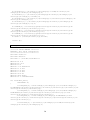
Nomenclature:
= radius vector,
̇ = velocity vector,
̈ = acceleration vector,
̂
̂
̂
= component of radius in ̂ ̂ or ̂ direction
= gravitational parameter of Earth,
= position in x direction,
= position in y direction,
= position in z direction,
̇ = velocity in x direction,
̇ = velocity in y direction,
̈ = acceleration in x direction,
̈ = acceleration in y direction,
̈ = acceleration in z direction,
= mean motion of the reference orbit,
= initial position in x direction,
= initial position in y direction,
̇ = initial velocity in x direction,
̇ =initial velocity in y direction,
= time,
= radius vector,
= Origin
= True Anomaly,
̂ ̂ = in plane inertial reference frame
2
̂ ̂ = in plane relative reference frame
P '  m ' = Earth
R
= position of spacecraft with respect to Earth, m
aˆn
= orbit-fixed reference frame
bˆn
= body-fixed reference frame
n
= angular velocities, rad/s
n
= initial angular velocities, rad/s
n
= angular acceleration, rad/s2
n
= quaternions
n
= quaternions derivatives
J
= axial moment of inertia, kg-m2
I
= lateral moment of inertia, kg-m2

= mean motion, rad/s
s
= spin input, rad/s
̂
= Euler axis

= Euler angle, deg
n
= angular velocities, rad/s
n
= initial angular velocities, rad/s
n
= angular acceleration, rad/s2
Kn
= ratio of moments of inertia
n
= quaternions
n
= initial quaternions
n
= quaternions derivatives
J
= axial moment of inertia of the rotor, kg-m2
In
= lateral moment of inertia of the spacecraft, kg-m2

= mean motion, rad/s
0
0
0
3
s
= spin input, rad/s
B
A
= rotor speed, rad/s
t
= time, s

= number of orbits

= standard gravitational parameter, m3/s2
R
= radius, m
m
= mass, kg
r
= radius of rotor, m
aˆn
= orbit-fixed reference frame
bˆn
= body-fixed reference frame
n
0
B
A

= initial angular velocities, rad/s
= rotor speed, rad/s
= nutation angle, deg
4
1. Introduction
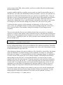
Class Background
The project was the result of a two-semester course. During the first semester, the basics of Trick
and C were introduced. The second semester brought the introduction to the visualization
package (AVIZO) and the project work. Through the project, programming skills in Trick and C
were further developed. Through this project, attitude dynamics and orbit mechanics we
combined in order to see the combined effect. Since one was affecting the other and vice versa,
the system had to be investigated as a whole. The effect of attitude on orientation and the effect
of orientation on drag and attitude both had to be included.
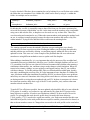
Team Focus
The scope of the project was very open ended in order to allow each team to concentrate on what
the students were more interested in. The red team originally decided to focus on fuel efficiency
by optimizing the rendezvous path of two spacecraft. This proved to be difficult to do given the
time constraints, since a variety of methods had to be investigated, so it was changed. The new
focus aimed to determine the ΔV necessary to transfer orbits based on the location of application
along the initial orbit.
Team Goals
The initial goal of the team was to determine the focus for the semester. Throughout the semester
two experiments were carried out that helped the team navigate towards the end result.
More specifically, there were two sides to the project; one was model simulation and the other
was visualization. In terms of simulation, the equations for attitude and the orbit had to be
determined. Individual models for attitude and orbit were created and tested, before they had to
be put together in order to work with each other. For visualization purposes, the main goal
involved linking Trick and AVIZO in order to visualize the maneuvers modeled in real time.
Additionally, through this project, SVN version control was developed for the team to use in
order to work on code simultaneously.
5
2. SVN Version Control
In a group there are multiple codes that are shared and exchanged, and it is always important to
have the most updated code. SVN is a version control system that enables collaborative editing
and sharing of data. The first step to setup SVN for a new project is to use the command:
svnadmin create path_to_repository/PROJECT_FOLDER_NAME (Eg: svnadmin create
/home/lagrange/a/marchand_files/class_files/team_files/redteam/satellite_sim).
Now that a new project is created team members will want to check out satellite_sim to add and
share code, but before team members can checkout satellite_sim, it is important that permission
is given to the other team members. This was one of the first complications that red team
encountered when setting up SVN. This problem was solved by talking to other teams with SVN
working. The easy solution to this problem is to change the file mode (chmod –R 775
satellite_sim) and to change the group ownership (chgrp –R jsctrick satellite_sim), performing
both of these commands in the folder that contains satellite_sim. –R allows the files and
directories to change recursively, and 775 (or gtw) grants permission to other users who are
members of the files group, sets up restricted deletion flag or sticky bit, and allows the group to
write to the file. Changing the group to jsctrick, is an easier solution than manually trying to add
team members to the group, since everyone who has access to trick are part of the group jsctrick.
When adding team members manually, team members were still unable to checkout files.
Although changing the group to jsctrick works, it does not restrict other teams from accessing
red team’s folders.
Now that team members have access to satellite_sim, the next step is to check out the folder.
When checking out files, it is helpful to have a folder that contains SVN projects (mkdir
MySVNProjects). Within MySVNPorjects folder, use the command: svn checkout
file:///path_to_repository/PROJECT_FOLDER_NAME (Eg: svn checkout
file:///home/lagrange/a/marchand_files/class_files/team/files/redteam/satellite_sim/). A new
SVN project only needs to be checked out once.
Now with a checked out version of satellite_sim, files can be imported or added to it. Most svn
commands are similar to C, except with the addition of svn (svn mv, svn rm, svn mkdir, etc.).
Typing svn help in the command window will display the possible commands that can be
performed in SVN. For more information on a particular SVN command, type svn help
subcommand (svn help mv). One method of adding files to SVN is to use the command: svn
import path_to_your_code file://path_to_repository/PROJECT_FOLDER_NAME -m
“Description”
(Eg: svn import trick_sims/SIM_orbit/
file:///home/lagrange/a/marchand_files/class_files/team_files/redteam/satellite_sim/) –m
“Simulation for two spacecrafts in orbit”). The problem with using svn import is that all the files
in the imported file name are sent to satellite_sim except for the folder that was holding those
files. For example, importing SIM_orbit will add all the files that are in SIM_orbit (S_define,
RUN_test, Modified_data, etc.), but it will not import SIM_orbit. This problem can be fixed by
6
easily creating a folder SIM_orbit in satellite_sim first (svn mkdir SIM_orbit) and then import
the files in that location.
An easier method to add files to satellite_sim is to simily copy the files into satellite_sim (cp –r
$HOME/trick_sims/SIM_orbit $HOME/MySVNProjects/satellite_sim/trick_sims) and then svn
add these files within the folder that these files were copied to (svn add SIM_orbit). Using svn
add makes it easier to format and organize the files that are added. With multiple team members
and code, it is important to make SVN as user friendly as possible. Added files need to be
organized in a manner that is easy to find. Red team set up satellite_sim so that it is very similar
to working in your own directories adding trick_models, trick_sims, and a Trick_profile.
To delete files from a project, use the command: svn delete name_of_file or svn rm --force
name_of_file. The command svn delete is mainly used for deleting a single file, while svn rm –
force is used for folders. When making a change like deleting a file, that change must be
committed.
There are times when the files are not all added or deleted from svn because of a warning or
restriction, or maybe a team member wants to add and overwrite a code that had previously been
added to svn. Useful commands in these situations are svn add --force file_name and svn delete -force file_name. Thankfully at times svn will let you know when commands need to be forced
like the example below.
svn: Use --force to override this restriction
svn: 'anomaly.c~' is not under version control
By force adding and deleting it will overwrite/add/delete files without any problems. It should be
noted though that using these commands is permanent. Once a file is force deleted than it is gone
for that team member’s copy of the code.
After making any changes to the project (added new files, deleted files, altered files), the changes
need to be committed. To commit a change, use the command: svn commit –m “Description
about what was changed”. It is important Before and after committing changes it is important to
see which version of the project you are at by doing svn update. With multiple team members
making changes at the same time, it is important that both of you are not trying to commit
changes to the same file at the same time. Using the command svn info gives more information
about the latest version, and svn diff –r 2:1 shows the changes that were made between the two
versions with 2 for example being the second version and one being the first version. It is very
important to get in the habitat of committing a file right after adding it. Problems can arise if
multiple changes are being made in different folders and they have not been committed yet.
If a mistake is made, those changes can be undone by using svn revert, but this command only
effects local changes and does not undo changes that have already been committed. To undo
changes that have already been committed, it is useful to use the command: svn merge –c -2
name_of_file (svn merge –c -2 cannon_deriv.c).
7
It can be checked if files have been committed to svn by looking for a .svn file that exists within
the folder that you committed. It is a hidden file, which can be seen by using ls –a within the
folder. An example can be seen below.
. anomaly.c
.svn
.. atmospheric.c
hohmann_complete.c
orbit_deriv.c
orbit_integ.c
hohmann_init.c
orbit_init.c
rel_pos.c
By deleting the .svn file, it essentially removes those files from svn. Our team experienced an
error with svn because of the hidden .svn file. At the time not all the members were comfortable
using svn to add or delete files, so dropbox was also used as a way to share files. These files
were then taken and committed to svn. When other team members tried running the updated code
on svn, it would not compile properly because the other team members did not have any files
within attitude2. Trying to force add this folder would cause the warning below.
svn: warning: 'spacecraft/attitude2/src' is already under version control
The warning appeared because the attitude2 files that were put on dropbox were already
committed to svn from a previous revision. Finding the hidden .svn file helped determine this,
and this problem was resolved by deleting .svn and then properly adding the files to the most
updated revision. This error was a clear example of the problems that can occur when team
members are using different methods to store or update code like dropbox.
When adding a simulation file, it is very important that only the necessary files are added and
committed to the project (Modefied_data, Run_test, S_define). Multiple problems will occur if
CP_out and the extra files are not removed. Red team encountered this problem after running a
simulation within satellite_sim, and then trying to make changes to that simulation. When red
team tried to commit a change, an error message would appear and say that CP_out conflicts
with these changes. To fix this problem SIM_orbit was deleted and then added again, but this
time only committing the necessary files. It is also important to know that there is a hidden file
.auto_checksums within the simulation file and files in RUN_test that will also cause problems
unless they are removed. Sometimes after fixing all the errors there are still team members that
are having trouble receiving the most updated code on SVN. In these circumstances it is best to
have that team member delete their copy of the SVN code (satellite_sim), and have that team
member recheck-out these files.
To make SVN as efficient as possible, the most updated code should be able to be run within the
SVN project. It would be very tedious to copy and transfer files from the SVN project to the
home directory to run files. In order to run simulations within SVN, there needs to be a trick
profile. To accomplish this task, the trick profile that is located in the home directory
(.Trick_profile_07.23.1) needs to be copied into satellite_sim. Each team member has their own
individual trick profile, so the trick profile that was copied to satellite_sim needs to be altered, so
that each team member can use it. Changes that were made to the trick profile can be seen below.
TRICK_HOME="/home/lagrange/a/marchand_files/trick/07.23.1" ; export TRICK_HOME
8
TRICK_USER_HOME="$HOME/MySVNProjects/satellite_sim/trick_sims" ; export
TRICK_USER_HOME
TRICK_CATALOG_HOME="$HOME/MySVNProjects/satellite_sim/trick_catalog" ; export
TRICK_CATALOG_HOME
TRICK_USER_PROFILE="$HOME/MySVNProjects/satellite_sim/.Trick_user_profile" ;
export TRICK_USER_PROFILE
TRICK_CFLAGS="$TRICK_CFLAGS -I$HOME/MySVNProjects/satellite_sim/trick_models"
The trick profile located in the home directory is still what is going to be used when running a
simulation unless the user switches to the trick profile that was created in satellite_sim. Users can
switch their trick profiles by using the command source Trick_profile_07.23.1. Another more
permanent method of changing trick profiles is to alter the .bashrc file. The very first line of the
.bashrc file is source ~/.Trick_profile_07.23.1. By changing the path from the home trick profile
to the one created in SVN, simulations can be run in satellite_sim without having to do source
Trick_profile_07.23.1.
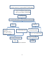
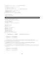
An overview for setting up SVN and using basic commands like adding and deleting files can be
seen in figure 1.
9
svnadmin create path_to_repository/PROJECT_FOLDER_NAME
chmod –R 775 PROJECT_FOLDER_NAME
chgrp –R jsctrick PROJECT_FOLDER_NAME
mkdir MySVNProjects
svn checkout file:///path_to_repository/PROJECT_FOLDER_NAME
Delete Files
Add Files
svn add FOLDER_NAME
svn import
path_to_your_code
file:///path_to_repositor
y
/PROJECT_FOLDER_
NAME -m
“Description”
svn delete FILE_NAME
svn rm --force FOLDER_NAME
svn commit –m “Description”
svn commit –m “Description”
svn update
svn update
Figure 2.1: SVN Overview
10
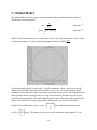
3. Orbital Model
The orbital model used in the project was calculated by the gravitational inverse square law
which can be seen in equation 1.
̈
‖ ‖
Where ̈ is the acceleration vector,
is shown in equation 2;
Equation 1[3]
‖ ‖
√
̂
Equation 2[3]
̂
̂
is the radius vector, ‖ ‖ is the norm of the vector
is the gravitational parameter which is
and it
.
Figure 3.1: Circular Orbit plotted using Trick
The bold lettering signifies a vector with ̂, ̂ and ̂ components. These vectors are in the IJK
inertial reference frame where the center of Earth is at [0, 0, 0]. To use this equation initial
conditions must be specified, namely a position vector and velocity vector. For simplification an
initial position could be specified where it is only in one direction, therefore the velocity will
also be in only one direction. The initial radius from the center of the origin will be equal to the
radius of the Earth,
, along with the altitude above the surface of the Earth.
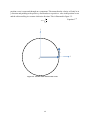
In figure 2 the initial radius vector is
is ̇ ( )
[
]
( )
[
]
and the initial velocity vector
. The initial velocity vector can be calculated using equation 3, as its
11
position vector is expressed through an x component. This means that the velocity will only be in
y direction and pointing to the positive y direction due to a positive x value in the position vector
and the orbit travelling in a counter-clockwise direction. This is illustrated in figure 3.2.
Equation 3 [2]
√
𝑗̂
𝑟̇
𝑖̂
𝑂
Figure 3.2: Circular Orbit with axis and vectors
12
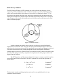
Hill-Clohessy-Wiltshire
The Hill-Clohessy-Wiltshire (HCW) equations are used to calculate the change in velocity
required to perform a Hohmann transfer. A Hohmann transfer is a transfer of 180 degrees that
can be used to reach a higher orbit or drop to a lower orbit. It is illustrated in figure 3.3. The
figure shows the parking orbit which is an initial orbit, the transfer orbit and the mission orbit
which is the final orbit. The dot that connects the initial orbit and the transfer orbit is referred to
as the Periapsis of the transfer orbit and the point at which the transfer orbit intersects the final
orbit is called the Apoapsis.
Figure 3.3: Hohmann Transfer [1]
In order to initiate the transfer orbit, an increase in velocity is required and must be
tangential to the initial orbit. This will create an elliptical orbit and the Periapsis will be at the
point where the velocity was increased. If the spacecraft does not make any changes in velocity it
will remain on the transfer orbit, passing through the Periapsis and Apoapsis indefinitely.
Another change in velocity is required in order to circularize the orbit so that it will remain in the
final orbit. This change in velocity is required to be implemented at the Apoapsis which is 180
degrees from the Periapsis.
The HCW equations will be used to calculate the changes in velocity required in order to
successfully transfer into the final orbit. The HCW equations are derived from equations of
motion below:
̈
Equation 4 [2]
̇
̈
̇
Equation 5 [2]
Equation 6 [2]
̈
This derivation is only considering in plane motion and z is uncoupled, therefore it is not
considered in this derivation
13
∫( ̈
̇)
̇
̇
̇
̇
Substitute into equation (4)
̈
̇
̈
̇
̇
( )
̇
(
( )
)
̇
̇
̇
( )
̇
(
̇
( )
)
Equation 7
Substitute into equation for ̇
̇
̇
[
̇
∫ ̇
̇
̇
∫
( )
(
( )
(
( )
̇
( )
̇
̇
̇ )
( )
̇ )
(
̇ )
̇
( )
( )
]
̇
( )
̇ )
(
̇
( )
)
(
̇
( )
̇
̇
̇
Equation 8
(
̇ )
Equation 7 and 8 are the general solution, however, as the spacecraft will be travelling
along a Hohmann transfer, it is safe to assume
. The general equations will now simplify
to equation 9 and 10.
14
̇
Equation 9
̇
Equation 10
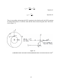
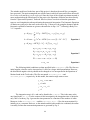
There is one problem when using the HCW equations in the orbital model; the HCW equations
are defined in the frame of a reference orbit and this frame rotates along this orbit. This can be
seen in figure 3.4.
Figure 3.4:
a) Hohmann transfer with relative frame b) Hohmann transfer viewed from reference orbit
15
[2]
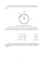
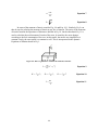
This means that there will need to be a conversion from the reference frame into the
inertial frame. It will be done by taking figure 4a and combining it with the inertial frame in
figure 3.5.
𝑗̂
𝑥̂
𝒓
𝜃
𝑦̂
𝑖̂
𝑂
Figure 3.5: Inertial frame with reference frame
Now it is possible to define the relative frame in terms of the inertial frame. This is
shown in equations 8 and 9. After this it is possible to rearrange these equations so that the
inertial frame can be defined through the reference frame, which is shown in equations 13 and
14.
̂
( ) ̂
( )̂
Equation 11
̂
( )̂
( )̂
Equation 12
( )̂
( )̂
Equation 13
( )̂
( )̂
Equation 14
̂
̂
In order to convert the relative change in velocity that was calculated using the HCW
equations into the inertial IJK frame, the relative velocity in the ̂ and ̂ directions are multiplied
by the corresponding term in equation 13 and 14. The output will therefore be in the ̂ and ̂
components.
16
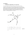
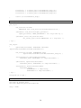
4. Attitude
- Axisymmetric Rigid Body in Circular Orbit
The attitude model used in the earlier part of this project is based on the model for the
axisymmetric cylindrical spacecraft. The main assumptions are that all spacecraft follow the
model for circular orbit and drag can be neglected. In general, there are two types of cylindrical
spacecraft, namely the rod spacecraft and the disk spacecraft. The first experiment has concluded
that the orientation of the rod spacecraft is more unstable as compared to that of the disk
spacecraft. Hence, the disk configuration is chosen for this experiment as seen in Fig. 4.1.
Moreover, the dynamic and the kinematic equations of motion are given as shown below in
equations. 1-3 [4], following a Body Two 3-1-3 sequence.
Figure 4.1: This is the disk spacecraft on a circular orbit [2].


J

1   s2  1   23  12 2  1 2   3 4  31   2 4  
I


J

2  s1  1   13  6 2  31   2 4  1  2 22  2 32  
I
3  0
17
Equation 1
21   2 3  s      32   41
2 2   31   42  1 3  s   
2 3   4 3  s     12   21
Equation 2
2 4  11   22   3 3  s   
s  30  
Equation 3
The governing factors between the rod and the disk spacecraft are the axial and the lateral
moments of inertia. In general, for the former case, the value of I is less than the value of J. On
the other hand, for the latter case, the value of J is less than the value of I. There are no integrator
tolerances in Trick’s Runge_Kutta_4 and this is not something that is expected [6]. In terms of
the results, Figs. 4.2 and 4.3 below show the behavior of the quaternions after performing
numerical integration with respect to time for an equivalent of two orbits.
18
Figure 4.2: This is the rod spacecraft attitude quaternions.
19
Figure 4.3: This is the disk spacecraft attitude quaternions.
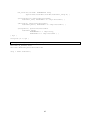
The main things to be noted in coding the Trick part are the constants and the initial
conditions. As mentioned earlier, it is evident that the axial and the lateral moments of inertia are
to be kept constant. However, in reality, this would change as the spacecraft performs orbital
maneuvers and thus reducing the amount of fuel. Moreover, the Ω and the s terms are also kept
constant as shown in Fig. 4.5. In terms of the initial conditions, the term ω3 is set to 6 rad/s.
Moreover, the initial nutation angle is set to 8 deg, which affects the initial values of the
quaternions.
20
/* Default data for attitude 1 */
ATTITUDE1.omega0[0]
ATTITUDE1.omega0[1]
ATTITUDE1.omega0[2]
ATTITUDE1.euler0[0]
ATTITUDE1.euler0[1]
ATTITUDE1.euler0[2]
ATTITUDE1.euler0[3]
{r/s}
{r/s}
{r/s}
{--}
{--}
{--}
{--}
=
=
=
=
=
=
=
0;
0;
6;
0;
0.069756473744125;
0;
0.997564050259824;
Figure 4.4: These are the initial conditions of the spacecraft attitude as coded in Trick.
#define JJ 184078
#define II 136217
#define OM 0.00116
#define SS 5.99884
Figure 4.5: These are the constants used throughout the numerical integration scheme.
21
The attitude model used in the later part of this project is based on the model for a rectangular
box spacecraft. The main assumptions are still the same in which all spacecraft follow the model
for circular orbit and drag can be neglected. Since the focus of the second experiment onward is
more emphasized on the orbital aspect of the project, the Equations of Motion are taken directly
from the “Spacecraft Dynamics” textbook. However, these were derived into the quaternion
terms to avoid singularities when performing the numerical integration. The kinematic Equations
of Motion are going to be the same as the one in Eq. 2. Moreover, the complete dynamic and the
kinematic equations of motion are given as shown below in Eqs. 4-6 [4], following a Body Two
3-1-3 sequence.
1  K123 
J A B
 2  12 2 K1  1 2   3 4  31   2 4 
I1
2  K 231 
J A B
 1  6 2 K 2  31   2 4  1  2 22  2 32 
I2
Equation 4
3  K312  6 2 K3 1  2 22  2 32   1 2   3 4 
21   2 3  s      32   41
2 2   31   42  1 3  s   
2 3   4 3  s     12   21
Equation 5
2 4  11   22   3 3  s   
s  30  
Equation 6
The following initial conditions are then specified in the attitude2.d file. The first two
initial angular velocities can be increased to 0.1 rad/s for a larger initial perturbation. However,
the third initial angular velocity should not be changed as it is incorporated in the Equations of
Motion found in the Trick codes. The files are named attitude2_init.c and
attitude2_deriv.c, respectively. In this model, the nutation angle starts at zero.
1  2  0.05 rad/s
0
0
3  1 rad/s
0
1   2   3  0
0
0
0
4  1
0
The integration step is 0.1 s and can be found in the S_define. This is the same as the
one found in the dre.tcl. For the context of this investigation, the integration time is limited to
only 3000 s. In theory, Eq. 4 governs the time parameter as a function of the number of orbits.
Moreover, in the attitude2_init.c and the attitude2_deriv.c files, the mean motion Ω is
initially set as a constant. However, as the attitude and the orbit models are combined, the radius
is actually fed into the mean motion parameter as governed by Eq. 8.
22
2

t
Equation 7


Equation 8
R3
In terms of the moment of inertia, consider Fig. 4.6 and Eqs. 9-11. Similarly, Eq. 9 can
then be used to calculate the moment of inertia at any face of interest. The ratios of the moments
of inertia found in the Equations of Motion are defined in Eq. 10. On the other hand, Eq. 11 is
used to calculate the axial moment of inertia of the rotor. In actuality, the mass changes
according to the fuel consumption. However, in this model, the masses are simplified as a
constant. Lastly, the rotor speed is a constant as well. This is incorporated in the dynamic
Equations of Motion shown in Eq. 1.
Figure 4.6: This is a guideline to calculate the moments of inertia.
I1 
K1 
I 2  I3
,
I1
m 2
x  y2 

12
K2 
J
I 3  I1
,
I2
mr 2
2
23
Equation 9
K3 
I1  I 2
I3
Equation 10
Equation 11
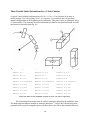
Three Possible Initial Orientations for a 3-Unit CubeSat
A typical 3-unit CubeSat has dimensions of 0.1 m × 0.1 m × 0.3 m. In terms of its mass, it
usually weighs 3 kg. Using a Body Two 3-1-3 sequence, it is possible to have at least three
attitude configurations in the beginning of the simulation. These three cases are illustrated in Fig.
4.7 shown below. The moments of inertia information can then be calculated and found to be the
ones shown in the subsequent Fig. 4.8.
Figure 4.7: This figure shows the three possible initial orientations where the orbit normal is out of the page.
#define K1 0
#define K1 -0.8
#define K1 0.8
#define K2 0.8
#define K2 0
#define K2 -0.8
#define K3 -0.8
#define K3 0.8
#define K3 0
#define JJ 0.000253125
#define JJ 0.000253125
#define JJ 0.000253125
#define I1 0.005
#define I1 0.025
#define I1 0.025
#define I2 0.025
#define I2 0.005
#define I2 0.025
#define I3 0.025
#define I3 0.025
#define I3 0.005
#define SG 0.05
#define SG 0.05
#define SG 0.05
Figure 4.8: These are the simulation constants for cases A, B, and C, respectively.
The relationship between the terms K1 and K2 can then be plotted on the instability chart.
The shaded regions indicate unstable or unknown behaviors [7]. Due to the CubeSat being more
symmetric than a typical rectangular spacecraft, these three cases fall on the borderline between
24
certain regions as shown in Fig. 9. The results of the numerical integration are also shown in Fig.
4.10. At this stage, one may predict that case C is going to yield the more stable result.
Figure 4.9: This is the instability chart with the depicted cases A, B, and C.
Figure 4.10: These are the quaternions plots for cases A, B, and C, respectively.
A better way to represent the stability behavior is to plot the nutation angles for each case
using Eqs. 12 and 13 [5] subsequently. These angles are plotted as shown in Fig. 4.11. Both cases
A and B have nutation angles up to 180 deg whereas case C only goes up to 10 deg and thus
being the more stable case. Another test on these approaches is to turn off the rotation of the
rotor using extreme initial conditions, such as 5 rad/s for the first two angular velocities. As seen
in Fig. 4.12, the nutation angle reduces to 85 deg when the rotor is turned off for the first 3000 s.
On the other hand, the nutation angle reduces to 80 deg when the rotor is spun at 10 rad/s for the
first 3000 s.
25
C33  1  212  2 22
Equation 12
  cos1  C33 
Equation 13
Figure 4.11: These are the nutation angles for cases A, B, and C, respectively.
Figure 4.12: These are the nutation angles in testing the effect of the rotor for case C.
26
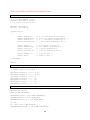
Simulating Attitude in AVIZO
For the visualization purposes, these quaternions need to be converted into Euler axis and
Euler angle. This is because the visualization package AVIZO only works with this scheme [7].
To begin with, the parameters defined in Eqs. 14 and 15 [2] is introduced in the header file. It
should be noted that these Euler axis and Euler angles are defined in the orbit frame. The lines
shown in Fig. 4.13 are then added to both the initialization and the derivative files. In the end,
these two additional parameters are then added to the linking code.
ˆ 
1aˆ1   2 aˆ2   3aˆ3

2
1
 
2
2
1
2 2
3

  2cos1  4 
Equation 14
Equation 15
A->lambda[0] = A->euler[0]/pow(A->euler[0]*A->euler[0]+A->euler[1]*A>euler[1]+A->euler[2]*A->euler[2],0.5);
A->lambda[1] = A->euler[1]/pow(A->euler[0]*A->euler[0]+A->euler[1]*A>euler[1]+A->euler[2]*A->euler[2],0.5);
A->lambda[2] = A->euler[2]/pow(A->euler[0]*A->euler[0]+A->euler[1]*A>euler[1]+A->euler[2]*A->euler[2],0.5);
A->theta = (2*acos(A->euler[3]))/PI*180;
Figure 4.13: These lines convert the quaternions into Euler axis and Euler angle
27
5. Experiment 1
Hypothesis
If a rod-like spacecraft is used, then an equivalent stability will be observed as if a disk-like
spacecraft was used. A spacecraft with higher moment of inertia will be as stable as one with a
lower moment of inertia.
Prediction
The particles in a cylindrical object within a gravitational field will experience a gravity gradient
between the top and bottom halves due to gravity being stronger at the bottom than at the top.
Theoretically, this would mean that a slight deviation from the gravitation vector – here defined
as the vertical orientation - would result in a torque for the object. A longer object would have a
higher torque, and therefore be more unstable. However, we predict that for a certain range of
values this torque is negligible and has little significant effect – no more than 1o nutation angle
variation. We predict this since the variation in gravitational field is extremely small over the
span of a nano satellite scale object.
Formally, we state our prediction as such: there is no significant (+-1o variation in nutation
angle) difference in stability between an object with a moment of inertia of 327364 and one of
644125.
Experiment
The equations used to define the moment of inertia I and the second moment of inertia J for a
cylindrical object are shown below (Equations 1 & 2).
mr 2
2
(1)
m
3r 2  h 2 

12
(2)
J
I
To describe a variation of shape from a long, thin cylinder to a wide, flat disk, a range of both
moments of inertia were used (Table 5.1, Figure 5.1).
28
No. r [m] h [m] V [m3] m [kg] I [kgm2] J [kgm2]
1
4.5
1
64 63617 327364 644125
2
3.5
2
77 76969 261374 471435
3
2.5
3
59 58905 136217 184078
4
1.5
4
28 28274
53603
31809
5
0.5
5
4
3927
8427
491
Table 5.1: Experimental Initial Conditions
Figure 5.1: Variation of Satellite Shape
Using the above as well as the initial conditions given in Table 5.2 and the constants given in
Table 5.3, several simulations were carried to find the time history of nutation angle in the
system described by the equations of motion below (Equation 3).
1  0
2 
2



J

  s3   I  1   13  12  1 2   3 4   2 3  1 4   




3 
2


 J
 2 s   1  I




2
2
  12  6  1 2   3 4  1  2 3  21  




29
(3)
Variable
Initial Condition
ω1
6 rad/s
ω2
0 rad/s
ω3
0 rad/s
ε1
0
ε2
0
ε3
0.06975647374
ε4
0.9975640503
ν
8 degrees
Table 5.2: Initial Conditions
Constant
Value
π
3.141592
Ω
0.00116
Table 5.3: Constants
The simulation was run for two full orbits for each of the five different objects, and the nutation
angle history for each was recorded.
30
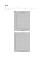
Results
The spacecraft was varied from the disk shape to a rod shape by the same increments in both
radius and height. Figures 2 to 6 below show the nutation angle over a period of two orbits for
this variation.
Figure 5.2. First Spacecraft
Figure 5.3. Second Spacecraft
31
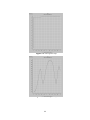
Figure 5.4. Third Spacecraft
Figure 5.5. Fourth Spacecraft
32
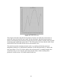
Figure 5.6. Fifth Spacecraft
These figures show that when the lateral moment of inertia is less than the axial moment of
inertia, the spacecraft would be more stable. On the other hand, when the lateral moment of
inertia is more than the axial moment of inertia, the spacecraft would be unstable with deviations
of nutation angle significantly greater than 1o. This observation also shows that the stable forms
did not differ from each other and also true for the unstable cases.
The ratio between these moments of inertia can be very similar such that the numerical
integration resulted in very similar Euler parameters. For the disk spacecraft (i.e. stable), this
ratio varied from 1.35 to 1.80. In the contrary, the rod spacecraft (i.e. unstable) had the ratio
varied from 0.06 to 0.59. Using the same body reference frame, similar resulting Euler
parameters would result in very similar nutation behaviors.
33
Conclusion
In conclusion, we reject our null hypothesis that a variation of moment of inertia will result in an
insignificant change in inherent stability of an orbiting satellite. When the ratio of moments of
inertia is greater than one, the spacecraft is stable. A ratio of moments of inertia less than one
results in an unstable satellite. This indicates that any modeling of rendezvousing satellites would
be greatly eased by choosing a craft with a lower lateral, and a higher axial moment of inertia. It
was noted that there is little difference in the magnitude of instability by varying the ratio of
moments of inertia once an object becomes unstable. Likewise, there is little variation in the
nutation angle history between the stable conditions with variation of the ratio of moments of
inertia. Therefore it can also be concluded that the satellite need only have a ratio of moments
larger than one in order to simplify the rendezvous process. This can be done either through the
modification of the shape of the satellites or through altering their initial orientation. This means
that in order for a successful rendezvous the satellites would be best off being put in mutually
stable attitudes through the use of on board controls before attempting to connect to one another.
From this experiment we can conclude that this stable attitude would exist where the ratio of
moments of inertia is greater than one, or where the satellite is lying “flat”, or normal to its
orbital plane in the case of a long cube-satellite.
34
6. Experiment 2
Hypothesis
Given two spacecraft in low Earth orbit, the Hill-Clohessy-Wiltshire (HCW) equations are
accurate in predicting the velocity required to transfer a spacecraft from an eccentric orbit into a
circular orbit.
Introduction
Initially both spacecraft will be in low Earth orbit at an altitude of 250km, where the radius of
the Earth is 6378.14 km and the gravitational constant is 398600.4418 km3/s2[1]. In this
experiment the two spacecraft will be released at the same position with slightly different
velocities. One spacecraft will remain in a circular orbit at an altitude of 250 km and another will
have a velocity slightly less than the circular velocity at 250 km and will therefore have an
eccentric orbit. The Hohmann transfer is going to be implemented to transfer the spacecraft from
the initial position to the circular orbit as this transfer is the most fuel efficient. The HCW
equations will be used to calculate the initial velocity required to implement the Hohmann
transfer and this initial velocity will be used in the Trick through the inverse square law equation
of motion. There is an error when using the velocity calculated in the HCW equations in the
inverse square law model. This experiment will look at the effect of increasing the initial relative
velocity on the final position that is calculated using the inverse square law.
35
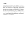
Procedure
To determine the accuracy of the HCW equations, the difference in the initial relative velocities
between the two orbits are shown in Table 1. Each trial will use the HCW equations to calculate
the initial velocity required to for the two spacecraft to rendezvous, recording the error between
them at the end of the transfer. The error from each trial will be compared to the expected
position of a circular orbit. This will determine the overall accuracy of the HCW equations.
Table 1 shows the trials that are run for the experiment.
Trial
Initial
Position in ̂
(km)
Initial Velocity
of spacecraft
in eccentric
orbit (km/s)
Initial Velocity
of spacecraft in
circular orbit
(km/s)
1
-6628.14
7.7547
7.7548
2
-6628.14
7.7546
7.7548
3
-6628.14
7.7545
7.7548
4
-6628.14
7.7544
7.7548
5
-6628.14
7.7543
7.7548
6
-6628.14
7.7542
7.7548
7
-6628.14
7.7541
7.7548
8
-6628.14
7.7540
7.7548
9
-6628.14
7.7539
7.7548
10
-6628.14
7.7538
7.7548
Table 6.1: Inputs of the Experiment
A visual representation of the procedure can be seen in Figure 3. After each trial, the initial
relative velocity on the elliptical orbit is decreased, changing the shape of the ellipse, while the
velocity for spacecraft on the circular orbit remains constant.
36
Figure 6.1: Visual representation of the Procedure
In this experiment the difference in the initial relative velocity is the independent variable and
the error between the two spacecraft after using HCW equations is the dependent variable.
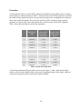
Experiment
The initial velocity of the first spacecraft decreased by 0.1 m/s after each trial, while the initial
velocity for the second spacecraft remains constant at 7.7548 km/s (circular velocity with a radial
distance of 6,628.14 km.
The plots from the experiment can be seen in Figures 4-12.
37
Figure 6.2: Change in Initial Velocity (km/s): -0.005 m/s
38
Figure 6.3: Change in Initial Velocity (km/s): -0.025 m/s
39
Figure 6.3: Change in Initial Velocity (km/s): -0.05 m/s
40
Figure 6.4: Change in Initial Velocity (km/s): -0.1 m/s
41
Figure 6.5: Change in Initial Velocity (km/s): -0.4 m/s
42
Figure 6.6: Change in Initial Velocity (km/s): -1 m/s
43
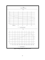
2000
Magnitude Seperation (m)
1800
1600
1400
1200
1000
800
600
400
200
0
-1.2
-1
-0.8
-0.6
-0.4
-0.2
0
Difference in Initial Velocities (m/s)
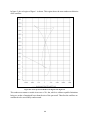
Figure 6.7: Quarter Orbit Seperation against Difference in Initial Velocities
250
Post Transfer error (m)
200
150
100
50
0
-1.2
-1
-0.8
-0.6
-0.4
-0.2
0
Difference in Initial Velocities (m/s)
Figure 6.8: Post Transfer Error against Difference in Initial Velocities
44
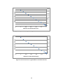
8.4
Seperation/Error Ratio
8.3
8.2
8.1
8
7.9
7.8
7.7
7.6
0
2
4
6
8
10
12
14
Difference in Initial Velocities (m/s)
Figure 6.9: Ratio of Pre-Transfer Seperation to Post-Transfer Error
As can be seen, there is a persistent error that exists in a simulated Hohmann transfer using
velocities found through the HCW equations. This error decreases nonlinearly with initial
separation distance (or the difference in release velocities of the cubesats). This suggests that in
order to get a complete rendezvous using the HCW approximations, it is necessary to perform
multiple burns, each at minimum relative distance.
Conclusion
It is evident that as the difference in velocities between the two spacecraft is increased, the final
position of the transfer is not on the circular orbit, where it should be. This shows that there is an
error introduced when using the velocity calculated through the HCW equations in an inverse
square gravity environment. This has disproven our hypothesis and the HCW equations cannot
predict the velocity required to transfer.
45
7. Visualization
Linking Trick to Avizo 7.0
The aim of linking Trick to Avizo is to be able to visualize the simulations in real time. Prior to
the link, Avizo would use predetermined data stored in the .hx file to visualize the different
movements associated with an object. Now the data is no longer in the .hx file - instead it doesn’t
even exist, until the visualization starts communicating with Trick in order to retrieve the data.
The ‘serverconnect.scro’ file was developed in order to establish the link between the numerical
simulation and its visualization. It requires the IP address of the server running the simulation
and the port number in order to retrieve the data. In order to retrieve the right data, the variables
assigned in the .dre file are recalled.
The command used to obtain the IP address of the server in UNIX is displayed below
accompanied by an example.
46
$ /sbin/ifconfig
eth0
Link encap:Ethernet HWaddr 00:22:19:0F:9D:BB
inet addr:128.46.105.20 Bcast:128.46.105.255 Mask:255.255.255.0
inet6 addr: fe80::222:19ff:fe0f:9dbb/64 Scope:Link
UP BROADCAST RUNNING MULTICAST MTU:1500 Metric:1
RX packets:443071472 errors:0 dropped:1 overruns:0 frame:3470
TX packets:541776189 errors:0 dropped:0 overruns:0 carrier:0
collisions:0 txqueuelen:1000
RX bytes:268726588892 (250.2 GiB) TX bytes:523436942266 (487.4 GiB)
Interrupt:33
lo
Link encap:Local Loopback
inet addr:127.0.0.1 Mask:255.0.0.0
inet6 addr: ::1/128 Scope:Host
UP LOOPBACK RUNNING MTU:16436 Metric:1
RX packets:187943867 errors:0 dropped:0 overruns:0 frame:0
TX packets:187943867 errors:0 dropped:0 overruns:0 carrier:0
collisions:0 txqueuelen:0
RX bytes:235149938192 (219.0 GiB) TX bytes:235149938192 (219.0 GiB)
Figure 7.1: Obtaining the IP address in UNIX
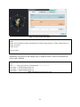
In order to find the port number, the simulation should be called first. The Simulation Control
Panel will appear, and it will need to be maximized before the port number can be viewed at the
bottom. An example can be seen below.
Figure 7.2: Finding the port number for the simulation
Before starting the simulation, the RealTime button needs to be unclicked so that the simulation
does not take 24 hours to run. Instead, it will be accelerated. Alternatively, the throttle can be
used to control the speed of the simulation. The throttle can be found under the Actions menu.
47
set hideNewModules 0
create HxScriptObject "serverconnect.scro"
"serverconnect.scro" script setValue ${SCRIPTDIR}/serverconnect.scro
Note: The previous lines place a new module in the pool, name it “serverconnect.scro” and calls the .scro module
with the same name, found in the same directory as the .hx file.
"serverconnect.scro" setIconPosition 285 158
"serverconnect.scro" setVar "scroTypeTranslateObject" {1}
"serverconnect.scro" setVar "scroTypeTranslateObject" {1}
"serverconnect.scro" fire
"serverconnect.scro" time setMinMax 1 300
"serverconnect.scro" time setSubMinMax 1 300
"serverconnect.scro" time setValue 1
"serverconnect.scro" time setDiscrete 0
"serverconnect.scro" time setIncrement 1
"serverconnect.scro" time animationMode -once
"serverconnect.scro" ipAddress setState 128.46.105.20
"serverconnect.scro" portNumber setState 7000
Note: The two lines above assign default values to the ‘ipAddress’ and ‘portNumber’ boxes in the module
properties. It is important to note that the values set in the .hx file will override any values that are already set in the
.scro script.
"serverconnect.scro" targName setState Object.wrl
"serverconnect.scro" targName2 setState Object2.wrl
Note: The two lines above change the names of the objects that will be moved based on the simulation results.
"serverconnect.scro" cycle_rate setState 1
"serverconnect.scro" numberSteps setState 100
"serverconnect.scro" applyTransformToResult 1
"serverconnect.scro" fire
"serverconnect.scro" setViewerMask 65535
"serverconnect.scro" select
"serverconnect.scro" setPickable 1
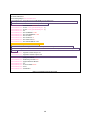
Figure 7.3: Annotated script for the .hx file
48
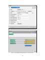
Figure 1.4: The Properties box of the serverconnect.scro module with values assigned from the .hx file
Figure 7.5: The arrangement of the models and the serverconnect.scro module
49
One Spacecraft
To simulate and visualize one spacecraft in orbit around the Earth, the ‘serverconnect.scro’ file
had to first be developed and included in the simulation file. The .hx file of the simulation was
edited in order to include the new module, but also to assign the parameters in the properties box
of the module.
The script shown below connects to Trick and retrieves the data in the dyn.orbit.pos and the
dyn.orbit.vel vectors. The velocity is not currently used in the visualization, but the position
vector is used to display the position of the object that is in orbit.
simcom_send_cmd $sat(socket) "var_cycle = $cycle_rate;"
simcom_send_cmd $sat(socket) "var_add dyn.orbit.pos\[0\];"
simcom_send_cmd $sat(socket) "var_add dyn.orbit.pos\[1\];"
simcom_send_cmd $sat(socket) "var_add dyn.orbit.pos\[2\];"
simcom_send_cmd $sat(socket) "var_add dyn.orbit.vel\[0\];"
simcom_send_cmd $sat(socket) "var_add dyn.orbit.vel\[1\];"
simcom_send_cmd $sat(socket) "var_add dyn.orbit.vel\[2\];"
Figure 7.6: Retrieving data from Trick
The following while loop then gets the data from Trick and saves it in sim_data in the
appropriate format.
while { [gets $sat(socket) sim_data] != -1} {
set sat(positions) $sim_data; # [format "%.0f" $sim_data]
Figure 7.7: Saving data in sim_data
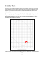
The next task was to translate the object using the command setTranslation <x> <y> <z>. This is
identical to manually translating an object from the transformation dialog window, however now
the script does it automatically and it updates constantly so that a continuous movement can be
observed.
50
Figure 7.8: The Transform Editor Dialog
update
Phobos.wrl setTranslation [lindex $sat(positions) 0] [lindex $sat(positions) 1] [lindex $sat(positions) 2]
Phobos.wrl touch 1
Phobos.wrl fire
viewer 0 redraw
Figure 7.9: Translating object
Additionally, the position of the orbiting object is displayed on the Console so that numerical
values can be validated.
# echo "$sat(positions)"
echo " "
echo "---------Step [expr $counter - $timeInt(min)]---------------------"
echo "target x = [lindex $sat(positions) 0]"
echo "target y = [lindex $sat(positions) 1]"
echo "target z = [lindex $sat(positions) 2]"
Figure 7.10: Displaying position in the Console
51
Multiple Spacecraft
In order to add a second spacecraft in a different object, the ‘serverconnect.scro’ file had to be
edited in order to now start getting more variables from the Trick simulation.
simcom_send_cmd $sat(socket) "var_cycle = $cycle_rate;"
simcom_send_cmd $sat(socket) "var_add dyn.orbit.pos\[0\];"
simcom_send_cmd $sat(socket) "var_add dyn.orbit.pos\[1\];"
simcom_send_cmd $sat(socket) "var_add dyn.orbit.pos\[2\];"
simcom_send_cmd $sat(socket) "var_add dyn.orbit2.pos\[0\];"
simcom_send_cmd $sat(socket) "var_add dyn.orbit2.pos\[1\];"
simcom_send_cmd $sat(socket) "var_add dyn.orbit2.pos\[2\];"
Figure 7.11: Retrieving position data for two spacecraft
The position data of the two spacecraft is stored in adjacent positions in the array, with the first
spacecraft data coming first. The correct elements have to be used each time when translating the
different spacecraft, as shown below.
update
phobos.wrl setTranslation [lindex $sat(positions) 0] [lindex $sat(positions) 1] [lindex $sat(positions) 2]
phobos.wrl touch 1
phobos.wrl fire
update
phobos2.wrl setTranslation [lindex $sat(positions) 3] [lindex $sat(positions) 4] [lindex $sat(positions) 5]
phobos2.wrl touch 1
phobos2.wrl fire
Figure 7.12: Translating two spacecraft
52
Attitude
In order to include attitude in the visualization model, the Trick simulation had to be edited so
that it would output two new parameters that Avizo needs in order to vary the attitude of the
object: the axis of a simple rotation in a 3-element vector format and the rotation angle in
degrees.
The object in Avizo is rotated about the specified axis of rotation using the same method as for
translation. The setRotation <x> <y> <z> <angle> command is used to change the attitude of the
spacecraft.
simcom_send_cmd $sat(socket) "var_cycle = $cycle_rate;"
simcom_send_cmd $sat(socket) "var_add dyn.orbit.pos\[0\];"
simcom_send_cmd $sat(socket) "var_add dyn.orbit.pos\[1\];"
simcom_send_cmd $sat(socket) "var_add dyn.orbit.pos\[2\];"
simcom_send_cmd $sat(socket) "var_add dyn.orbit2.pos\[0\];"
simcom_send_cmd $sat(socket) "var_add dyn.orbit2.pos\[1\];"
simcom_send_cmd $sat(socket) "var_add dyn.orbit2.pos\[2\];"
simcom_send_cmd $sat(socket) "var_add attitude1.euler\[0\];"
simcom_send_cmd $sat(socket) "var_add attitude1.euler\[1\];"
simcom_send_cmd $sat(socket) "var_add attitude1.euler\[2\];"
simcom_send_cmd $sat(socket) "var_add attitude1.euler\[3\];"
simcom_send_cmd $sat(socket) "var_add attitude1.euler2\[0\];"
simcom_send_cmd $sat(socket) "var_add attitude1.euler2\[1\];"
simcom_send_cmd $sat(socket) "var_add attitude1.euler2\[2\];"
simcom_send_cmd $sat(socket) "var_add attitude1.euler2\[3\];"
simcom_send_cmd $sat(socket) "var_add dyn.orbit.vel\[0\];"
simcom_send_cmd $sat(socket) "var_add dyn.orbit.vel\[1\];"
simcom_send_cmd $sat(socket) "var_add dyn.orbit.vel\[2\];"
simcom_send_cmd $sat(socket) "var_add dyn.orbit2.vel\[0\];"
simcom_send_cmd $sat(socket) "var_add dyn.orbit2.vel\[1\];"
simcom_send_cmd $sat(socket) "var_add dyn.orbit2.vel\[2\];"
serverconnect.scro script
#####################################################################
#----------------------constructor----------------------------------#
# Script used to connect Trick and Avizo #
#####################################################################$
$this proc constructor {} {
clear
echo "********************************************************************"
53
echo " Sat_connect program"
echo "********************************************************************"
echo ""
echo " To run simulation, start the Trick simulator first,"
echo " but do not hit start until after the 'Retrieve Data'"
echo " button in Avizo is pressed."
# scro "ID"
$this setVar scroTypeTranslateObject 1
# Set global variables for access outside of constructor
#global sat
global xPositionT
global yPositionT
global zPositionT
# Empties variables
set xPositionT "0"
set yPositionT "0"
set zPositionT "0"
# master time slider
$this newPortTime time
$this time setMinMax 1 300
$this time setIncrement 1
# IP Address Box
$this newPortText ipAddress
$this ipAddress setLabel "Server IP Address: "
$this ipAddress setNumColumns 30
$this ipAddress setValue "127.0.0.1"
# Port Number Box
$this newPortText portNumber
$this portNumber setLabel "Port Number"
$this portNumber setNumColumns 6
$this portNumber setValue 7000
# Creates the text field for entering the object names
# phobos.wrl
$this newPortText targName
$this targName setLabel "Name of Spacecraft:"
$this targName setValue "phobos.wrl"
# phobos2.wrl
$this newPortText targName2
$this targName2 setLabel "Name of Spacecraft:"
$this targName2 setValue "phobos2.wrl"
# rate to read data from server
$this newPortText cycle_rate
$this cycle_rate setLabel "Read time interval:"
$this cycle_rate setNumColumns 5
$this cycle_rate setValue 1
# Total Number of Steps
$this newPortText numberSteps
$this numberSteps setLabel "Total Iterations"
$this numberSteps setNumColumns 6
$this numberSteps setValue 100
# Retrieve Data Button
$this newPortButtonList openSocket 1
$this openSocket setLabel "Connection:"
$this openSocket setLabel 0 "Retrieve Data"
$this openSocket setCmd 0 {
set timecall [$this cycle_rate getValue]
global sat
global timeInt
global xPositionT
54
global yPositionT
global zPositionT
# connect to server
set sat(socket) [simcom_connect [$this ipAddress getValue] [$this portNumber getValue]]
get_sim_data $timecall [$this targName getValue]
$this numberSteps setValue $timeInt(max)
$this time setMinMax 1 $timeInt(max)
}
}
#########################################################$
#---------------get_sim_data----------------------------#$
# collects data from the server and defines it #$
#########################################################$
proc get_sim_data {cycle_rate phobos.wrl} {
global sat
global timeInt
global xPositionT
global yPositionT
global zPositionT
simcom_send_cmd $sat(socket) "var_cycle = $cycle_rate;"
simcom_send_cmd $sat(socket) "var_add dyn.orbit.pos\[0\];"
simcom_send_cmd $sat(socket) "var_add dyn.orbit.pos\[1\];"
simcom_send_cmd $sat(socket) "var_add dyn.orbit.pos\[2\];"
simcom_send_cmd $sat(socket) "var_add dyn.orbit2.pos\[0\];"
simcom_send_cmd $sat(socket) "var_add dyn.orbit2.pos\[1\];"
simcom_send_cmd $sat(socket) "var_add dyn.orbit2.pos\[2\];"
simcom_send_cmd $sat(socket) "var_add attitude1.euler\[0\];"
simcom_send_cmd $sat(socket) "var_add attitude1.euler\[1\];"
simcom_send_cmd $sat(socket) "var_add attitude1.euler\[2\];"
simcom_send_cmd $sat(socket) "var_add attitude1.euler\[3\];"
simcom_send_cmd $sat(socket) "var_add attitude1.euler2\[0\];"
simcom_send_cmd $sat(socket) "var_add attitude1.euler2\[1\];"
simcom_send_cmd $sat(socket) "var_add attitude1.euler2\[2\];"
simcom_send_cmd $sat(socket) "var_add attitude1.euler2\[3\];"
simcom_send_cmd $sat(socket) "var_add dyn.orbit.vel\[0\];"
simcom_send_cmd $sat(socket) "var_add dyn.orbit.vel\[1\];"
simcom_send_cmd $sat(socket) "var_add dyn.orbit.vel\[2\];"
simcom_send_cmd $sat(socket) "var_add dyn.orbit2.vel\[0\];"
simcom_send_cmd $sat(socket) "var_add dyn.orbit2.vel\[1\];"
simcom_send_cmd $sat(socket) "var_add dyn.orbit2.vel\[2\];"
set counter 0
set timeInt(min) 0
set timeInt(max) 0
if { [gets $sat(socket) sim_data] == -1 } { echo " Thats all folks..." }
while { [gets $sat(socket) sim_data] != -1} {
set sat(positions) $sim_data; # [format "%.0f" $sim_data]
if {[lindex $sat(positions) 0]==0} {
set timeInt(min) [expr $counter+1]
echo "Waiting for Trick"
update
55
} else {
# Appends data to lists
lappend xPositionT "[lindex $sat(positions) 0]"
lappend yPositionT "[lindex $sat(positions) 1]"
lappend zPositionT "[lindex $sat(positions) 2]"
lappend xPositionT "[lindex $sat(positions) 3]"
lappend yPositionT "[lindex $sat(positions) 4]"
lappend zPositionT "[lindex $sat(positions) 5]"
update
phobos.wrl setTranslation [lindex $sat(positions) 0] [lindex $sat(positions) 1] [lindex $sat(positions) 2]
phobos.wrl setRotation [lindex $sat(positions) 6] [lindex $sat(positions) 7] [lindex $sat(positions) 8] [lindex
$sat(positions) 9]
phobos.wrl touch 1
phobos.wrl fire
update
phobos2.wrl setTranslation [lindex $sat(positions) 3] [lindex $sat(positions) 4] [lindex $sat(positions) 5]
phobos.wrl setRotation [lindex $sat(positions) 6] [lindex $sat(positions) 7] [lindex $sat(positions) 8] [lindex
$sat(positions) 9]
phobos2.wrl touch 1
phobos2.wrl fire
viewer 0 redraw
# echo "$sat(positions)"
echo " "
echo "---SC1------Step [expr $counter - $timeInt(min)]---------------------"
echo "target x = [lindex $sat(positions) 0]"
echo "target y = [lindex $sat(positions) 1]"
echo "target z = [lindex $sat(positions) 2]"
echo "e1 = [lindex $sat(positions) 6]"
echo "e2 = [lindex $sat(positions) 7]"
echo "e3 = [lindex $sat(positions) 8]"
echo "angle = [lindex $sat(positions) 9]"
# echo "$sat(positions)"
echo " "
echo "---SC2------Step [expr $counter - $timeInt(min)]---------------------"
echo "target x = [lindex $sat(positions) 3]"
echo "target y = [lindex $sat(positions) 4]"
echo "target z = [lindex $sat(positions) 5]"
echo "e1 = [lindex $sat(positions) 6]"
echo "e2 = [lindex $sat(positions) 7]"
echo "e3 = [lindex $sat(positions) 8]"
echo "angle = [lindex $sat(positions) 9]"
}
set counter [expr $counter + 1]
set timeInt(max) [expr $counter - $timeInt(min)]
}
}
##########################################################
#-------------destructor---------------------------------#
# destructor is called when scro is destroyed #
##########################################################
$this proc destructor {} {}
#####################################################################
#--------------------compute----------------------------------------#
# the "compute" method is called whenever a port has changed #
#####################################################################
$this proc compute {} {
56
# when the time slider is touched, translate object
if [$this time isNew] {
set tminmax [$this time getMinMax]
$this translateObject [$this targName getValue] [$this time getValue] [lindex $tminmax 0] [lindex $tminmax 1]
}
}
############################################################################
#----------------translateObject-------------------------------------------#
# translate attached object $obj between two positions, corresponding to #
# time step $t within $t_minmax. #
############################################################################
$this proc translateObject {objSatellite t tmin tmax} {
#repeat for Satellite
if {$objSatellite == ""} {
echo "$this: no data Satellite object connected."
$this data disconnect
return
}
if {![$objSatellite hasInterface HxSpatialData]} {
$echo "$this: $objSatellite is not a spatial data object."
$this data disconnect
return
}
# Let procedure know to look in global namespace
global xPositionT
global yPositionT
global zPositionT
# Drop down to the lat integer of timestep
set floorTime [expr floor([$this time getValue])]
set intTime [expr int($floorTime)]
# Set the translation/rotation values
set xSatellite [lindex $xPositionT $intTime]
set ySatellite [lindex $yPositionT $intTime]
set zSatellite [lindex $zPositionT $intTime]
# preform the translation/rotation
$objSatellite setTranslation $xSatellite $ySatellite $zSatellite
$objSatellite touch 1;
$objSatellite fire
}
##############################################################################
# USER: DO NOT EDIT!!!! #
##############################################################################
proc simcom_connect { host port } {
global simcom_error
global tcl_platform
set ret [catch { set sock [socket $host $port] } dog]
if { $ret != 0 } { return -1 }
fconfigure $sock -buffering none
fconfigure $sock -translation binary
# Send over endianess
if { $tcl_platform(byteOrder) == "littleEndian" } {
puts -nonewline $sock \x01\x00
} else {
puts -nonewline $sock \x00\x00
}
# set client id ( only used in error messages )
set client_id [binary format I 8675309]
57
# set client tag ( buffered to 80 bytes )
set client_tag [binary format a80 "var_client"]
puts -nonewline $sock $client_id$client_tag
# Read off the server's endianess read $sock 2
set simcom_error 0
return $sock;
}
proc simcom_send_cmd { sock cmd } {
global simcom_error
# Send command to variable server
regsub {\n} $cmd { } cmd
set cmd_len [binary format I [string length $cmd] ]
if { [catch {puts -nonewline $sock $cmd_len}] } {
set simcom_error 1
}
if { [catch {puts -nonewline $sock $cmd}] } {
set simcom_error 1
}
}
# EDITED TRICK SIMCOM PACKAGE END
# VIZLAB
##############################################################################
# USER: INSERT APPROPRIATE VARIABLES FROM TRICK
##############################################################################
58
8. Further Work
In order to achieve rendezvous, multiple impulses were needed. We implemented logic into the
TRICK simulation such that a quarter orbit after the release of the spacecraft, the chaser would
attempt to rendezvous with the target iteratively, doing multiple burns at the points of closest
relative position.
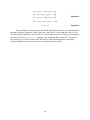
We ran several test cases, and were successful in all of them. In figure 1 the relative motion of
the spacecraft is shown for an initial difference in relative velocities of -10 m/s. The separation at
the time of the first impulse is 16.25 km. Figure 2 is in the orbital frame such that the earth is
positioned towards the negative x direction.
Figure 8.1: Relative Motion of Spacecraft With Respect to the Target, Initial Relative Velocity Separation of
-10 m/s
59
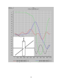
In figure 2, the red region of figure 1 is shown. This region shows the near-rendezvous behavior
of the satellites.
Figure 8.2: Close-up of Near-Rendezvous Region from Figure 8.1
This rendezvous maneuver results in an error of 10-5 km, which is within acceptable limitations
being two orders of magnitude lower than the size of the spacecraft. Therefore the satellites are
considered to be successfully rendezvoused.
60
9. Lessons Learned
Throughout the semester red team has learned multiple lessons that can be applied in the
workforce. Working in teams is inevitable in industry, and this class helped develop these team
working skills. Throughout the semester red team experienced common problems that happen
in teams: Lack of communication and multiple versions of code. Files were being stored on both
SVN and dropbox causing team members to have different versions of the code, and making it
difficult to know which version is the master code. These issues were resolved by simply
communicating with other team members.
In the entry level classes at Purdue there was a lot of emphasis on commenting code, and this
class was a great example why it is so important. Running a simulation requires multiple files,
and for each team member to fully understand the function of each file, it is important to
comment code as much as possible. When trying to debug code, it became difficult when the
purpose of an equation was unknown.
Team members have their own strengths and weaknesses and it is important to acknowledge
them. Tasks were split up among team members based on the classes that have been taken,
but sometimes after taking a class a student is constrained to think how they were taught from
a textbook or class notes. A team member with little experience in an area proved to be useful,
asking the right question that allowed our team to think outside the scope of the class and truly
understand how an equation is applied. Everyone thinks differently or goes about a problem in
a different way, and being open to a different point of view allows us to better understand the
problem. A great example of this is when red team was trying to use the Hill-Clohessy-Wiltshire
(HCW) Equations. To utilize these HCW equations in Trick, it required the team to understand
its limitations, the information that is needed to use it, and what information can be retrieved
from using these equations.
This class offered a lot of programming experience exposing the team to Trick simulations, TCL,
and applying C in Trick. Trying to visualize these simulations also required the team to learn
Avizo. Learning a new program or a new programming language can be difficult especially when
there are limited resources to learn it. Like everything else there is a learning curve. In the
workforce there will most likely be a new programming language that will have to be mastered.
The more exposure there is to different programs, the easier it will be to learn a new one.
Overall this class introduced red team to the lessons that would bed learned in industry,
allowing the team to learn from them at an early stage and know how to deal with these
problems when they are seen again in industry. This project allowed red team to apply our
classes in orbital mechanics and attitude dynamics and see how they interact. Having an idea is
great, but actually implanting it in code and visualizing it made the class worthwhile.
61
10. References
[1] Chobotv, V A 2002, Orbital Mechanics, 3rd edn, AIAA Education Series, VA, USA.
[2] Howell, K 2012, Orbit Mechanics Class Notes, Purdue University, West Lafayette, IN, USA.
[3] Curtis, H 2010, Orbital Mechanics for Engineering Students, 2nd edn, Elsevier, MA, USA.
[4] Kane, T. R. et al. (1983). Spacecraft Dynamics.
[5] Howell, K. C. (Spring 2012). Spacecraft Attitude Dynamics Class Notes.
[6] NASA Johnson Space Center Automation, Robotics and Simulation Division. (May 2008).
Trick User’s Guide.
[7] Brown, T. et al. (August 2011). Avizo the Supreme User’s Manual.
62
11. Appendix
Axisymmetric Rigid Body in Circular Orbit, Standalone Codes
/trick_models/spacecraft/attitude1/include/attitude1.h
/****** TRICK HEADER *******
PURPOSE: (Attitude 1 Header)
***************************/
#ifndef _attitude1_h_
#define _attitude1_h_
typedef struct
{
double
double
double
double
omega0[3];
omegadot0[3];
euler0[4];
eulerdot0[4];
/*
/*
/*
/*
*i r/s Init angular velocity */
r/s2 Init angular acceleration */
*i -- Init Euler parameters */
-- Init Euler parameters dot */
double
double
double
double
omega[3];
omegadot[3];
euler[4];
eulerdot[4];
/*
/*
/*
/*
r/s angular velocity */
r/s2 angular acceleration */
-- Euler parameters */
-- Euler parameters dot */
double
double
double
double
lambda0[3];
lambda[3];
theta0;
theta;
/*
/*
/*
/*
-- Init Euler axis */
-- Euler axis */
d Init Euler angle */
d Euler angle */
} ATTITUDE1;
#endif
/trick_models/spacecraft/attitude1/include/attitude1.d
/* Default data for attitude 1 */
ATTITUDE1.omega0[0]
ATTITUDE1.omega0[1]
ATTITUDE1.omega0[2]
ATTITUDE1.euler0[0]
ATTITUDE1.euler0[1]
ATTITUDE1.euler0[2]
ATTITUDE1.euler0[3]
{r/s}
{r/s}
{r/s}
{--}
{--}
{--}
{--}
=
=
=
=
=
=
=
0;
0;
6;
0;
0.069756473744125;
0;
0.997564050259824;
/trick_models/spacecraft/attitude1/include/attitude1_integ.d
#define NUM_STEP 12
#define NUM_VARIABLES 7
INTEGRATOR.state = alloc(NUM_VARIABLES);
INTEGRATOR.deriv = alloc(NUM_STEP);
INTEGRATOR.state_ws = alloc(NUM_STEP);
63
int kk;
for (kk = 0;kk < NUM_STEP;kk++) {
INTEGRATOR.deriv[kk] = alloc(NUM_VARIABLES);
INTEGRATOR.state_ws[kk] = alloc(NUM_VARIABLES);
}
INTEGRATOR.stored_data = alloc(8);
for (kk=0;kk < 8;kk++) {
INTEGRATOR.stored_data[kk] = alloc(NUM_VARIABLES);
}
INTEGRATOR.option = Runge_Kutta_4;
INTEGRATOR.init = True;
INTEGRATOR.first_step_deriv = Yes;
INTEGRATOR.num_state = NUM_VARIABLES;
#undef NUM_STEP
#undef NUM_VARIABLES
/trick_models/spacecraft/attitude1/src/attitude1_init.c
/******** TRICK HEADER *********
PURPOSE: (Initialize attitude 1)
*******************************/
#include <stdio.h>
#include <math.h>
#include "../include/attitude1.h"
#define
#define
#define
#define
JJ
II
OM
SS
184078
136217
0.00116
5.99884
int attitude1_init( /* RETURN: -- Always return zero */
ATTITUDE1* A) /* INOUT: -- Attitude 1 structure */
{
A->omega[0] = A->omega0[0];
A->omega[1] = A->omega0[1];
A->omega[2] = A->omega0[2];
A->omegadot[0] = -SS*A->omega[1]+(1-JJ/II)*(A->omega[1]*A->omega[2]12*OM*OM*(A->euler[0]*A->euler[1]-A->euler[2]*A->euler[3])*(A->euler[2]*A>euler[0]+A->euler[1]*A->euler[3]));
A->omegadot[1] = SS*A->omega[0]-(1-JJ/II)*(A->omega[0]*A->omega[2]6*OM*OM*(A->euler[2]*A->euler[0]-A->euler[1]*A->euler[3])*(1-2*pow(A>euler[1],2)-2*pow(A->euler[2],2)));
A->omegadot[2] = 0;
A->euler[0]
A->euler[1]
A->euler[2]
A->euler[3]
=
=
=
=
A->euler0[0];
A->euler0[1];
A->euler0[2];
A->euler0[3];
A->eulerdot[0] = (A->euler[1]*(A->omega[2]-SS+OM)-A->euler[2]*A>omega[1]+A->euler[3]*A->omega[0])/2;
64
A->eulerdot[1] = (A->euler[2]*A->omega[0]+A->euler[3]*A->omega[1]-A>euler[0]*(A->omega[2]-SS+OM))/2;
A->eulerdot[2] = (A->euler[3]*(A->omega[2]-SS-OM)+A->euler[0]*A->omega[1]A->euler[1]*A->omega[0])/2;
A->eulerdot[3] = (-A->euler[0]*A->omega[0]-A->euler[1]*A->omega[1]-A>euler[2]*(A->omega[2]-SS-OM))/2;
return (0);
}
/trick_models/spacecraft/attitude1/src/attitude1_deriv.c
/******** TRICK HEADER *********
PURPOSE: (Try Trick integration)
*******************************/
#include <stdio.h>
#include <math.h>
#include "../include/attitude1.h"
#define
#define
#define
#define
JJ
II
OM
SS
184078
136217
0.00116
5.99884
int attitude1_deriv(
ATTITUDE1* A)
{
A->omegadot[0] = -SS*A->omega[1]+(1-JJ/II)*(A->omega[1]*A->omega[2]12*OM*OM*(A->euler[0]*A->euler[1]-A->euler[2]*A->euler[3])*(A->euler[2]*A>euler[0]+A->euler[1]*A->euler[3]));
A->omegadot[1] = SS*A->omega[0]-(1-JJ/II)*(A->omega[0]*A->omega[2]6*OM*OM*(A->euler[2]*A->euler[0]-A->euler[1]*A->euler[3])*(1-2*pow(A>euler[1],2)-2*pow(A->euler[2],2)));
A->omegadot[2] = 0;
A->eulerdot[0] = (A->euler[1]*(A->omega[2]-SS+OM)-A->euler[2]*A>omega[1]+A->euler[3]*A->omega[0])/2;
A->eulerdot[1] = (A->euler[2]*A->omega[0]+A->euler[3]*A->omega[1]-A>euler[0]*(A->omega[2]-SS+OM))/2;
A->eulerdot[2] = (A->euler[3]*(A->omega[2]-SS-OM)+A->euler[0]*A>omega[1]-A->euler[1]*A->omega[0])/2;
A->eulerdot[3] = (-A->euler[0]*A->omega[0]-A->euler[1]*A->omega[1]-A>euler[2]*(A->omega[2]-SS-OM))/2;
return (0);
}
/trick_models/spacecraft/attitude1/src/attitude1_integ.c
/******** TRICK HEADER *********
PURPOSE: (Try Trick integration)
*******************************/
#include "sim_services/include/integrator.h"
#include "../include/attitude1.h"
65
int attitude1_integ(
INTEGRATOR *I,
ATTITUDE1* A )
{
/* Load current states */
I->state[0] = A->omega[0];
I->state[1] = A->omega[1];
I->state[2] = A->omega[2];
I->state[3] = A->euler[0];
I->state[4] = A->euler[1];
I->state[5] = A->euler[2];
I->state[6] = A->euler[3];
/* Load derivates */
I->deriv[I->intermediate_step][0]
I->deriv[I->intermediate_step][1]
I->deriv[I->intermediate_step][2]
I->deriv[I->intermediate_step][3]
I->deriv[I->intermediate_step][4]
I->deriv[I->intermediate_step][5]
I->deriv[I->intermediate_step][6]
=
=
=
=
=
=
=
A->omegadot[0];
A->omegadot[1];
A->omegadot[2];
A->eulerdot[0];
A->eulerdot[1];
A->eulerdot[2];
A->eulerdot[3];
/* Call the Trick integrator */
integrate (I);
/* Unload new
A->omega[0] =
A->omega[1] =
A->omega[2] =
A->euler[0] =
A->euler[1] =
A->euler[2] =
A->euler[3] =
states */
I->state_ws[I->intermediate_step][0];
I->state_ws[I->intermediate_step][1];
I->state_ws[I->intermediate_step][2];
I->state_ws[I->intermediate_step][3];
I->state_ws[I->intermediate_step][4];
I->state_ws[I->intermediate_step][5];
I->state_ws[I->intermediate_step][6];
return (I->intermediate_step);
}
/trick_sims/SIM_attitude1/S_define
sim_object
{
sim_services/include:
EXECUTIVE exec (sim_services/include/executive.d) ;
(automatic) sim_services/input_processor:
input_processor( INPUT_PROCESSOR * IP = &sys.exec.ip ) ;
(automatic_last) sim_services/exec:
var_server_sync( Inout EXECUTIVE * E = &sys.exec ) ;
} sys ;
sim_object
{
spacecraft/attitude1: ATTITUDE1 attitude1
(spacecraft/attitude1/include/attitude1.d) ;
66
sim_services/include: INTEGRATOR integ
(spacecraft/attitude1/include/attitude1_integ.d) ;
(initialization) spacecraft/attitude1:
attitude1_init( ATTITUDE1* A = &dyn.attitude1 ) ;
(derivative) spacecraft/attitude1:
attitude1_deriv( ATTITUDE1* A = &dyn.attitude1 ) ;
(integration) spacecraft/attitude1:
attitude1_integ(
INTEGRATOR* I = &dyn.integ,
ATTITUDE1* A = &dyn.attitude1 ) ;
} dyn ;
integrate (0.1) dyn ;
/trick_sims/SIM_attitude1/RUN_test/input
#include "S_default.dat"
#include "Modified_data/attitude1.dr"
stop = 10833.078115827;
67
Three-Unit CubeSat in Circular Orbit, Standalone Codes
/trick_models/spacecraft/attitude2/include/attitude2.h
/****** TRICK HEADER *******
PURPOSE: (Attitude 2 Header)
***************************/
#ifndef _attitude2_h_
#define _attitude2_h_
typedef struct
{
double
double
double
double
omega0[3];
omegadot0[3];
euler0[4];
eulerdot0[4];
/*
/*
/*
/*
*i r/s Init angular velocity */
r/s2 Init angular acceleration */
*i -- Init Euler parameters */
-- Init Euler parameters dot */
double
double
double
double
omega[3];
omegadot[3];
euler[4];
eulerdot[4];
/*
/*
/*
/*
r/s angular velocity */
r/s2 angular acceleration */
-- Euler parameters */
-- Euler parameters dot */
double lambda[3];
double theta;
/* -- Euler axis */
/* d Euler angle */
} ATTITUDE2;
#endif
/trick_models/spacecraft/attitude2/include/attitude2.d
/* Default data for attitude 2 */
ATTITUDE2.omega0[0]
ATTITUDE2.omega0[1]
ATTITUDE2.omega0[2]
ATTITUDE2.euler0[0]
ATTITUDE2.euler0[1]
ATTITUDE2.euler0[2]
ATTITUDE2.euler0[3]
{r/s}
{r/s}
{r/s}
{--}
{--}
{--}
{--}
=
=
=
=
=
=
=
0.05;
0.05;
1;
0;
0;
0;
1;
/trick_models/spacecraft/attitude2/include/attitude2_integ.d
#define NUM_STEP 12
#define NUM_VARIABLES 7
INTEGRATOR.state = alloc(NUM_VARIABLES);
INTEGRATOR.deriv = alloc(NUM_STEP);
INTEGRATOR.state_ws = alloc(NUM_STEP);
int kk;
for (kk = 0;kk < NUM_STEP;kk++) {
INTEGRATOR.deriv[kk] = alloc(NUM_VARIABLES);
68
INTEGRATOR.state_ws[kk] = alloc(NUM_VARIABLES);
}
INTEGRATOR.stored_data = alloc(8);
for (kk=0;kk < 8;kk++) {
INTEGRATOR.stored_data[kk] = alloc(NUM_VARIABLES);
}
INTEGRATOR.option = Runge_Kutta_4;
INTEGRATOR.init = True;
INTEGRATOR.first_step_deriv = Yes;
INTEGRATOR.num_state = NUM_VARIABLES;
#undef NUM_STEP
#undef NUM_VARIABLES
/trick_models/spacecraft/attitude2/src/attitude2_init.c
/******** TRICK HEADER *********
PURPOSE: (Initialize attitude 2)
*******************************/
#include <stdio.h>
#include <math.h>
#include "../include/attitude2.h"
#define
#define
#define
#define
#define
#define
#define
#define
#define
#define
K1
K2
K3
JJ
I1
I2
I3
SG
OM
PI
0.8
-0.8
0
0.000253125
0.025
0.025
0.005
0.05
0.00116
3.1415926535897
int attitude2_init( /* RETURN: -- Always return zero */
ATTITUDE2* A) /* INOUT: -- Attitude 2 structure */
{
A->omega[0] = A->omega0[0];
A->omega[1] = A->omega0[1];
A->omega[2] = A->omega0[2];
A->omegadot[0] = K1*A->omega[1]*A->omega[2]-(JJ/I1)*SG*A->omega[1]12*OM*OM*K1*(A->euler[0]*A->euler[1]-A->euler[2]*A->euler[3])*(A->euler[2]*A>euler[0]+A->euler[1]*A->euler[3]);
A->omegadot[1] = K2*A->omega[2]*A->omega[0]-(JJ/I2)*SG*A->omega[0]6*OM*OM*K2*(A->euler[2]*A->euler[0]+A->euler[1]*A->euler[3])*(1-2*A>euler[1]*A->euler[1]-2*A->euler[2]*A->euler[2]);
A->omegadot[2] = K3*A->omega[0]*A->omega[1]-6*OM*OM*K3*(1-2*A->euler[1]*A>euler[1]-2*A->euler[2]*A->euler[2])*(A->euler[0]*A->euler[1]-A->euler[2]*A>euler[3]);
A->euler[0]
A->euler[1]
A->euler[2]
A->euler[3]
=
=
=
=
A->euler0[0];
A->euler0[1];
A->euler0[2];
A->euler0[3];
69
A->eulerdot[0] = (A->euler[1]*(A->omega[2]-1+2*OM)-A->euler[2]*A>omega[1]+A->euler[3]*A->omega[0])/2;
A->eulerdot[1] = (A->euler[2]*A->omega[0]+A->euler[3]*A->omega[1]-A>euler[0]*(A->omega[2]-1+2*OM))/2;
A->eulerdot[2] = (A->euler[3]*(A->omega[2]-1)+A->euler[0]*A->omega[1]-A>euler[1]*A->omega[0])/2;
A->eulerdot[3] = (-A->euler[0]*A->omega[0]-A->euler[1]*A->omega[1]-A>euler[2]*(A->omega[2]-1))/2;
A->lambda[0] = A->euler[0]/pow(A->euler[0]*A->euler[0]+A->euler[1]*A>euler[1]+A->euler[2]*A->euler[2],0.5);
A->lambda[1] = A->euler[1]/pow(A->euler[0]*A->euler[0]+A->euler[1]*A>euler[1]+A->euler[2]*A->euler[2],0.5);
A->lambda[2] = A->euler[2]/pow(A->euler[0]*A->euler[0]+A->euler[1]*A>euler[1]+A->euler[2]*A->euler[2],0.5);
A->theta = (2*acos(A->euler[3]))/PI*180;
return (0);
}
/trick_models/spacecraft/attitude2/src/attitude2_deriv.c
/******** TRICK HEADER *********
PURPOSE: (Try Trick integration)
*******************************/
#include <stdio.h>
#include <math.h>
#include "../include/attitude2.h"
#define
#define
#define
#define
#define
#define
#define
#define
#define
#define
K1
K2
K3
JJ
I1
I2
I3
SG
OM
PI
0.8
-0.8
0
0.000253125
0.025
0.025
0.005
0.05
0.00116
3.1415926535897
int attitude2_deriv(
ATTITUDE2* A)
{
A->omegadot[0] = K1*A->omega[1]*A->omega[2]-(JJ/I1)*SG*A->omega[1]12*OM*OM*K1*(A->euler[0]*A->euler[1]-A->euler[2]*A->euler[3])*(A->euler[2]*A>euler[0]+A->euler[1]*A->euler[3]);
A->omegadot[1] = K2*A->omega[2]*A->omega[0]-(JJ/I2)*SG*A->omega[0]6*OM*OM*K2*(A->euler[2]*A->euler[0]+A->euler[1]*A->euler[3])*(1-2*A>euler[1]*A->euler[1]-2*A->euler[2]*A->euler[2]);
A->omegadot[2] = K3*A->omega[0]*A->omega[1]-6*OM*OM*K3*(1-2*A>euler[1]*A->euler[1]-2*A->euler[2]*A->euler[2])*(A->euler[0]*A->euler[1]-A>euler[2]*A->euler[3]);
A->eulerdot[0] = (A->euler[1]*(A->omega[2]-1+2*OM)-A->euler[2]*A>omega[1]+A->euler[3]*A->omega[0])/2;
70
A->eulerdot[1] = (A->euler[2]*A->omega[0]+A->euler[3]*A->omega[1]-A>euler[0]*(A->omega[2]-1+2*OM))/2;
A->eulerdot[2] = (A->euler[3]*(A->omega[2]-1)+A->euler[0]*A>omega[1]-A->euler[1]*A->omega[0])/2;
A->eulerdot[3] = (-A->euler[0]*A->omega[0]-A->euler[1]*A->omega[1]-A>euler[2]*(A->omega[2]-1))/2;
A->lambda[0] = A->euler[0]/pow(A->euler[0]*A->euler[0]+A->euler[1]*A>euler[1]+A->euler[2]*A->euler[2],0.5);
A->lambda[1] = A->euler[1]/pow(A->euler[0]*A->euler[0]+A->euler[1]*A>euler[1]+A->euler[2]*A->euler[2],0.5);
A->lambda[2] = A->euler[2]/pow(A->euler[0]*A->euler[0]+A->euler[1]*A>euler[1]+A->euler[2]*A->euler[2],0.5);
A->theta = (2*acos(A->euler[3]))/PI*180;
return (0);
}
/trick_models/spacecraft/attitude2/src/attitude2_integ.c
/******** TRICK HEADER *********
PURPOSE: (Try Trick integration)
*******************************/
#include "sim_services/include/integrator.h"
#include "../include/attitude2.h"
int attitude2_integ(
INTEGRATOR *I,
ATTITUDE2* A )
{
/* Load current states */
I->state[0] = A->omega[0];
I->state[1] = A->omega[1];
I->state[2] = A->omega[2];
I->state[3] = A->euler[0];
I->state[4] = A->euler[1];
I->state[5] = A->euler[2];
I->state[6] = A->euler[3];
/* Load derivates */
I->deriv[I->intermediate_step][0]
I->deriv[I->intermediate_step][1]
I->deriv[I->intermediate_step][2]
I->deriv[I->intermediate_step][3]
I->deriv[I->intermediate_step][4]
I->deriv[I->intermediate_step][5]
I->deriv[I->intermediate_step][6]
=
=
=
=
=
=
=
A->omegadot[0];
A->omegadot[1];
A->omegadot[2];
A->eulerdot[0];
A->eulerdot[1];
A->eulerdot[2];
A->eulerdot[3];
/* Call the Trick integrator */
integrate (I);
/* Unload new
A->omega[0] =
A->omega[1] =
A->omega[2] =
A->euler[0] =
states */
I->state_ws[I->intermediate_step][0];
I->state_ws[I->intermediate_step][1];
I->state_ws[I->intermediate_step][2];
I->state_ws[I->intermediate_step][3];
71
A->euler[1] = I->state_ws[I->intermediate_step][4];
A->euler[2] = I->state_ws[I->intermediate_step][5];
A->euler[3] = I->state_ws[I->intermediate_step][6];
return (I->intermediate_step);
}
/trick_sims/SIM_attitude2/S_define
sim_object
{
sim_services/include:
EXECUTIVE exec (sim_services/include/executive.d) ;
(automatic) sim_services/input_processor:
input_processor( INPUT_PROCESSOR * IP = &sys.exec.ip ) ;
(automatic_last) sim_services/exec:
var_server_sync( Inout EXECUTIVE * E = &sys.exec ) ;
} sys ;
sim_object
{
spacecraft/attitude2: ATTITUDE2 attitude2
(spacecraft/attitude2/include/attitude2.d) ;
sim_services/include: INTEGRATOR integ
(spacecraft/attitude2/include/attitude2_integ.d) ;
(initialization) spacecraft/attitude2:
attitude2_init( ATTITUDE2* A = &dyn.attitude2 ) ;
(derivative) spacecraft/attitude2:
attitude2_deriv( ATTITUDE2* A = &dyn.attitude2 ) ;
(integration) spacecraft/attitude2:
attitude2_integ(
INTEGRATOR* I = &dyn.integ,
ATTITUDE2* A = &dyn.attitude2 ) ;
} dyn ;
integrate (0.1) dyn ;
/trick_sims/SIM_attitude2/RUN_test/input
#include "S_default.dat"
#include "Modified_data/attitude2.dr"
stop = 3000;
72