1
A Comparison of Two MCMC Algorithms for Hierarchical Mixture Models
Russell G. Almond⇤
Florida State University
Abstract
1
Introduction
Mixture models (McLachlan & Peel, 2000) are a frequently used method of unsupervised learning. They
sort data points into clusters based on just their values. One of the most frequently used mixture models
is a mixture of normal distributions. Often the mean
and variance of each cluster is learned along with the
classification of each data point.
Mixture models form an important class of
models for unsupervised learning, allowing
data points to be assigned labels based on
their values. However, standard mixture
models procedures do not deal well with rare
components. For example, pause times in
student essays have di↵erent lengths depending on what cognitive processes a student
engages in during the pause. However, instances of student planning (and hence very
long pauses) are rare, and thus it is difficult to estimate those parameters from a
single student’s essays. A hierarchical mixture model eliminates some of those problems, by pooling data across several of the
higher level units (in the example students)
to estimate parameters of the mixture components. One way to estimate the parameters of a hierarchical mixture model is to use
MCMC. But these models have several issues
such as non-identifiability under label switching that make them difficult to estimate just
using o↵-the-shelf MCMC tools. This paper
looks at the steps necessary to estimate these
models using two popular MCMC packages:
JAGS (random walk Metropolis algorithm)
and Stan (Hamiltonian Monte Carlo). JAGS,
Stan and R code to estimate the models and
model fit statistics are published along with
the paper.
As an example, Almond, Deane, Quinlan, Wagner, and
Sydorenko (2012) fit a mixture of lognormal distributions to the pause time of students typing essays as
part of a pilot writing assessment. (Alternatively, this
model can be described as a mixture of normals fit to
the log pause times.) Almond et al. found that mixture models seems to fit the data fairly well. The mixture components could correspond to di↵erent cognitive process used in writing (Deane, 2012) where each
cognitive process takes di↵erent amounts of time (i.e.,
students pause longer when planning, than when simply typing).
Key words: Mixture Models, Markov Chain Monte
Carlo, JAGS, Stan, WAIC
⇤
Paper presented at the Bayesian Application Workshop at Uncertainty in Artificial Intelligence Conference 2014, Quebec City,
Canada.
1
Mixture models are difficult to fit because they display a number of pathologies. One problem is component identification. Simply swapping the labels of
Components 1 and 2 produces a model with identical
likelihoods. Even if a prior distribution is placed on
the mixture component parameters, the posterior is
multimodal. Second, it is easy to get a pathological
solution in which a mixture component consists of a
single point. These solutions are not desirable, and
some estimation tools constrain the minimum size of
a mixture component (Gruen & Leisch, 2008). Furthermore, if a separate variance is to be estimated for
each mixture component, several data points must be
assigned to each component in order for the variance
estimate to have a reasonable standard error. Therefore, fitting a model with rare components requires a
large data size.
Almond et al. (2012) noted these limitations in
their conclusions. First, events corresponding to the
highest-level planning components in Deane (2012)’s
cognitive model would be relatively rare, and hence
would lumped in with other mixture components due
to size restrictions. Second, some linguistic contexts
(e.g., between Sentence pauses) were rare enough that
fitting a separate mixture model to each student would
not be feasible.
One work-around is a hierarchical mixture model. As
with all hierarchical models, it requires units at two
di↵erent levels (in this example, students or essays
are Level 2 and individual pauses are Level 1). The
assumption behind the hierarchical mixture model is
that the mixture components will look similar across
the second level units. Thus, the mean and variance of
Mixture Component 1 for Student 1 will look similar
to those for Student 2. Li (2013) tried this on some of
the writing data.
One problem that frequently arises in estimating mixture models is determining how many mixture components to use. What is commonly done is to estimate
models for K = 2, 3, 4, . . . up to some small maximum
number of components (depending on the size of the
data). Then a measure of model–data fit, such as AIC,
DIC or WAIC (see Gelman et al., 2013, Chapter 7), is
calculated for each model and the model with the best
fit index is chosen. These methods look at the deviance
(minus twice the log likelihood of the data) and adjust
it with a penalty for model complexity. Both DIC and
WAIC require Markov chain Monte Carlo (MCMC) to
compute, and require some custom coding for mixture
models because of the component identification issue.
This paper is a tutorial for replicating the method used
by Li (2013). The paper walks through a script written in the R language (R Core Team, 2014) which performs most of the steps. The actual estimation is done
using MCMC using either Stan (Stan Development
Team, 2013) or JAGS (Plummer, 2012). The R scripts
along with the Stan and JAGS models and some sample data are available at http://pluto.coe.fsu.edu/
mcmc-hierMM/.
2
Mixture Models
Let i 2 {1, . . . , I} be a set of indexes over the second level units (students in the example) and let
j 2 {1, . . . , Ji } be the first level units (pause events
in the example). A hierarchical mixture model is by
adding a Level 2 (across student) distribution over the
parameters of the Level 1 (within student) mixture
model. Section 2.1 describes the base Level 1 mixture
model, and Section 2.2 describes the Level 2 model.
Often MCMC requires reparameterization to achieve
better mixing (Section 2.3). Also, there are certain parameter values which result in infinite likelihoods. Sec2
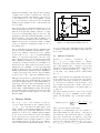
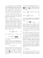
Figure 1: Non-hierarchical Mixture Model
tion 2.4 describes prior distributions and constraints
on parameters which keep the Markov chain away from
those points.
2.1
Mixture of Normals
Consider a collection observations,
Yi
=
(Yi,1 , . . . , Yi,Ji ) for a single student, i.
Assume
that the process that generated these data is a mixture of K normals. Let Zi,j ⇠ cat(⇡ i ) be a categorical
latent index variable indicating which component Ob⇤
servation j comes from and let Yi,j,k
⇠ N (µi,k , i,k )
be the value of Yi,j which would be realized when
Zi,j = k.
Figure 1 shows this model graphically. The plates indicate replication over categories (k), Level 1 (pauses,
j) and Level 2 (students, i) units. Note that there is
no connection across plates, so the model fit to each
Level 2 unit is independent of all the other Level 2
units. This is what Gelman et al. (2013) call the no
pooling case.
The latent variables Z and Y ⇤ can be removed from
the likelihood for Yi,j by summing over the possible
values of Z. The likelihood for one student’s data, Yi ,
is
Li (Yi |⇡ i , µi ,
i)
=
Ji X
K
Y
⇡i,k (
Yi,j
j=1 k=1
µi,k
)
(1)
i,k
where (·) is the unit normal density.
Although conceptually simple, there are a number of
issues that mixture models can have. The first issue is that the component labels cannot be identified
from data. Consider the case with two components.
The model created by swapping the labels for Components 1 and 2 with new parameters ⇡ 0i = (⇡i,2 , ⇡i,1 ),
µ0i = (µi,2 , µi,1 ), and 0i = ( i,2 , i,1 ) has an identical
likelihood. For the K component model, any permutation of the component labels produces a model with
identical likelihood. Consequently, the likelihood surface is multimodal.
A common solution to the problem is to identify the
components by placing an ordering constraint on one
of the three parameter vectors: ⇡, µ or . Section 4.1
returns to this issue in practice.
A second issue involves degenerate solutions which
contain only a single data point. If a mixture component has only a single data point, its standard deviation, i,k will go to zero, and ⇡i,k will approach 1/Ji ,
which is close to zero for large Level 1 data sets. Note
that if either ⇡i,k ! 0 or i,k > 0 for any k, then the
likelihood will become singular.
Estimating i,k requires a minimum number of data
points from Component k (⇡i,k Ji > 5 is a rough minimum). If ⇡i,k is believed to be small for some k, then a
large (Level 1) sample is needed. As K increases, the
smallest value of ⇡i,k becomes smaller so the minimum
sample size increases.
2.2
Hierarchical mixtures
Gelman et al. (2013) explains the concept of a hierarchical model using a SAT coaching experiment that
took place at 8 di↵erent schools. Let Xi ⇠ N (µi , i )
be the observed e↵ect at each school, where the school
specific standard error i is known (based mainly on
the sample size used at that school). There are three
ways to approach this problem: (1) No pooling. Estimate µi separately with no assumption about about
the similarity of µ across schools. (2) Complete pooling. Set µi = µ0 for all i and estimate µ0 (3) Partial pooling. Let µi ⇠ N (µ0 , ⌫) and now jointly estimate µ0 , µ1 , . . . , µ8 . The no pooling approach produces unbiased estimates for each school, but it has
the largest standard errors, especially for the smallest
schools. The complete pooling approach ignores the
school level variability, but has much smaller standard
errors. In the partial pooling approach, the individual
school estimates are shrunk towards the grand mean,
µ0 , with the amount of shrinkage related to the size of
the ratio ⌫ 2 /(⌫ 2 + i 2 ); in particular, there is more
shrinkage for the schools which were less precisely measured. Note that the higher level standard deviation,
⌫ controls the amount of shrinkage: the smaller ⌫ is
the more the individual school estimates are pulled towards the grand mean. At the limits, if ⌫ = 0, the partial pooling model is the same as the complete pooling
model and if ⌫ = 1 then the partial pooling model is
the same as the no pooling model.
Li (2013) builds a hierarchical mixture model for
the essay pause data. Figure 1 shows the no pool3
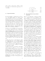
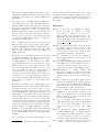
Figure 2: Hierarchical Mixture Model
ing mixture model. To make the hierarchical model,
add across-student prior distributions for the studentspecific parameters parameters, ⇡ i , µi and i . Because JAGS parameterizes the normal distribution
with precisions (reciprocal variances) rather than standard deviations, ⌧ i are substituted for the standard
deviations i . Figure 2 shows the hierarchical model.
Completing the model requires specifying distributions
for the three Level 1 (student-specific) parameters. In
particular, let
⇡ i = (⇡i,1 , . . . , ⇡i,K ) ⇠ Dirichlet(↵1 , . . . , ↵k )
µi,k ⇠ N (µ0,k ,
0,k )
log(⌧i,k ) ⇠ N (log(⌧0,k ),
0,k )
(2)
(3)
(4)
This introduces new Level 2 (across student) parameters: ↵, µ0 , 0 , ⌧ 0 , and 0 . The likelihood for a
single student, Li (Yi |⇡ i , µi , ⌧ i ) is given (with a suitable chance of variable) by Equation 1. To get the
complete data likelihood, multiply across the students
units (or to avoid numeric overflow, sum the log likelihoods). If we let ⌦ be the complete parameter (⇡ i ,µi ,
⌧ i for each student, plus ↵, µ0 , 0 , ⌧ 0 , and 0 ), then
L(Y|⌦) =
I
X
i=1
log Li (Yi |⇡ i , µi , ⌧ i ) .
(5)
Hierarchical models have their own pathologies which
require care during estimation. If either of the standard deviation parameters, 0,k or 0,k , gets too close
to zero or infinity, then this could cause the log posterior to go to infinity. These cases correspond to the no
pooling and complete pooling extremes of the hierarchical model. Similarly, the varianceP
of the Dirichlet
K
distribution is determined by ↵N = k=1 ↵k . If ↵N
is too close to zero, this produces no pooling in the
estimates of ⇡ i and if ↵N is too large, then there is
nearly complete pooling in those estimates. Again,
those values of ↵N can cause the log posterior to become infinite.
↵k = ↵0,k ⇤ ↵N
µi,k = µ0,k + ✓i,k
(6)
(7)
0,k
✓i,k ⇠ N (0, 1)
log(⌧i,k ) = log(⌧0,k ) + ⌘i,k
(8)
0,k
⌘i,k ⇠ N (0, 1)
2.3
Reparameterization
2.4
It is often worthwhile to reparameterize a model in order to make MCMC estimation more efficient. Both
random walk Metropolis (Section 3.2) and Hamiltonian Monte Carlo (Section 3.3) work by moving a point
around the parameter space of the model. The geometry of that space will influence how fast the Markov
chain mixes, that is, moves around the space. If the
geometry is unfavorable, the point will move slowly
through the space and the autocorrelation will be high
(Neal, 2011). In this case a very large Monte Carlo
sample will be required to obtain reasonable Monte
Carlo error for the parameter estimates.
Consider once more the Eight Schools problem where
µi ⇠ N (µ0 , ⌫). Assume that we have a sampler that
works by updating the value of the µi ’s one at a time
and then updating the values of µ0 and ⌫. When updating µi , if ⌫ is small then values of µi close to µ0 will
have the highest conditional probability. When updating ⌫ if all of the values of µi are close to µ0 , then small
values of ⌫ will have the highest conditional probability. The net result is a chain in which the movement
from states with small ⌫ and the µi ’s close together
to states with large ⌫ and µi ’s far apart takes many
steps.
A simple trick produces a chain which moves much
more quickly. Introduce a series of auxiliary variables
✓i ⇠ N (0, 1) and set µi = µ0 + ⌫✓i . Note that the
marginal distribution of µi has not changed, but the
geometry of the ✓, µ0 , ⌫ space is di↵erent from the geometry of the µ, µ0 , ⌫ space, resulting in a chain that
moves much more quickly.
A similar trick works for modeling the relationships
between ↵ and ⇡ i . Setting ↵k = ↵0,k ⇤ ↵N , where
↵0 has a Dirichlet distribution and ↵N has a gamma
distribution seems to work well for the parameters ↵ of
the Dirichlet distribution. In this case the parameters
have a particularly easy to interpret meaning: ↵0 is
the expected value of the Dirichlet distribution and ↵N
is the e↵ective sample size of the Dirichlet distribution.
Applying these two tricks to the parameters of the
hierarchical model yields the following augmented parameterization.
4
(9)
(10)
Prior distributions and parameter
constraints
Rarely does an analyst have enough prior information to completely specify a prior distribution. Usually, the analyst chooses a convenient functional form
and chooses the hyperparameters of that form based
on available prior information (if any). One popular
choice is the conjugate distribution of the likelihood.
For example, if the prior for a multinomial probability,
⇡ i follows a Dirichlet distribution with hyperparameter, ↵, then the posterior distribution will also be a
Dirichlet with a hyperparameter equal to the sum of
the prior hyperparameter and the data. This gives the
hyperparameter of a Dirichlet prior a convenient interpretation as pseudo-data. A convenient functional
form is one based on a normal distribution (sometimes
on a transformed parameter, such as the log of the
precision) whose mean can be set to a likely value of
the parameter and whose standard deviation can be
set so that all of the likely values for the parameter
are within two standard deviations of the mean. Note
that for location parameters, the normal distribution
is often a conjugate prior distribution.
Proper prior distributions are also useful for keeping
parameter values away from degenerate or impossible
solutions. For example, priors for standard deviations,
0,k and 0,k must be strictly positive. Also, the group
precisions for each student, ⌧ i , must be strictly positive. The natural conjugate distribution for a precision is a gamma distribution, which is strictly positive.
The lognormal distribution, used in Equations 4 and 9,
has a similar shape, but its parameters can be interpreted as a mean and standard deviation on the log
scale. The mixing probabilities ⇡ i must be defined
over the unit simplex (i.e., they must all be between 0
and 1 and they must sum to 1), as must the expected
mixing probabilities ↵0 ; the Dirichlet distribution satisfies this constraint and is also a natural conjugate.
Finally, ↵N must be strictly positive; the choice of the
chi-squared distribution as a prior ensures this.
There are other softer restraints on the parameters. If
0,k or 0,k gets too high or too low for any value of
k, the result is a no pooling or complete pooling solution on that mixture component. For both of these
parameters (.01, 100) seems like a plausible range. A
lognormal distribution which puts the bulk of its probability mass in that range should keep the model away
from those extremes. Values of ⌧i,k that are too small
represent the collapse of a mixture component onto
a single point. Again, if ⌧0,k is mostly in the range
(.01, 100) the chance of an extreme value of ⌧i,k should
be small. This yields the following priors:
⇠ N (0, 1)
(11)
log(⌧0k ) ⇠ N (0, 1)
(13)
log(
0k )
log(
0k )
⇠ N (0, 1)
(12)
High values of ↵N also correspond to a degenerate solution. In general, the gamma distribution has about
the right shape for the prior distribution of ↵N , and we
expect it to be about the same size as I, the number
of Level-2 units. The choice of prior is a chi-squared
distribution with 2 ⇤ I degrees of freedom.
↵N ⇠
2
(I ⇤ 2)
(14)
The two remaining parameters we don’t need to constrain too much. For µ0,k we use a di↵use normal
prior (one with a high standard deviation), and for ↵0
we use a Je↵rey’s prior (uniform on the logistic scale)
which is the Dirichlet distribution with all values set
to 1/2.
µ0,k ⇠ N (0, 1000)
↵0 ⇠ Dirichlet(0.5, . . . , 0.5)
(15)
(16)
The informative priors above are not sufficient to always keep the Markov chain out of trouble. In particular, it can still reach places where the log posterior
distribution is infinite. There are two di↵erent places
where these seem to occur. One is associated with high
values of ↵N . Putting a hard limit of ↵N < 500 seems
to avoid this problem (when I = 100). Another possible degenerate spot is when ↵k ⇡ 0 for some k. This
means that ⇡i,k will be essentially zero for all students.
Adding .01 to all of the ↵k values in Equation 2 seems
to fix this problem.
⇡ i = (⇡i,1 , . . . , ⇡i,K ) ⇠ Dirichlet(↵1 +.01, . . . , ↵k +.01)
3
Estimation Algorithms
There are generally two classes of algorithms used
with both hierarchical and mixture models. The expectation maximization (EM) algorithm (Section 3.1)
searches for a set of parameter values that maximizes
the log posterior distribution of the data (or if the prior
distribution is flat, it maximizes the log likelihood). It
5
comes up with a single parameter estimate but does
not explore the entire space of the distribution. In contrast, MCMC algorithms explore the entire posterior
distribution by taking samples from the space of possible values. Although the MCMC samples are not independent, if the sample is large enough it converges in
distribution to the desired posterior. Two approaches
to MCMC estimation are the random walk Metropolis
algorithm (RWM; used by JAGS, Section 3.2) and the
Hamiltonian Monte Carlo algorithm (HMC; used by
Stan, Section 3.3).
3.1
EM Algorithm
McLachlan and Krishnan (2008) provides a review of
the EM algorithm with emphasis on mixture models.
The form of the EM algorithm is particularly simple
for the special case of a non-hierarchical mixture of
normals. It alternates between an E-step where the
p(Zi,j = k) = pi,j,k is calculated for every observation,
j, and every component, k and an M-step where the
maximum likelihood values for ⇡i,k , µi,k and i,k are
found by taking moments of the data set Yi weighted
by the component probabilities, pi,j,k .
A number of di↵erent problems can crop up with using
EM to fit mixture models. In particular, if ⇡i,k goes to
zero for any k, that component essentially disappears
from the mixture. Also, if i,k goes to zero the mixture component concentrates on a single point. Furthermore, if µi,k = µi,k0 and i,k = i,k0 for any pair
of components the result is a degenerate solution with
K 1 components.
As the posterior distribution for the mixture model is
multimodal, the EM algorithm only finds a local maximum. Running it from multiple starting points may
help find the global maximum; however, in practice it
is typically run once. If the order of the components
is important, the components are typically relabeled
after fitting the model according to a predefined rule
(e.g., increasing values of µi,k ).
Two packages are available for fitting non-hierarchical
mixture models using the EM algorithm in R (R Core
Team, 2014): FlexMix (Gruen & Leisch, 2008) and
mixtools (Benaglia, Chauveau, Hunter, & Young,
2009). These two packages take di↵erent approaches
to how they deal with degenerate solutions. FlexMix
will combine two mixture components if they get too
close together or the probability of one component gets
too small (by default, if ⇡i,k < .05). Mixtools, on the
other hand, retries from a di↵erent starting point when
the the EM algorithm converges on a degenerate solution. If it exceeds the allowed number of retries, it
gives up.
Neither mixtools nor FlexMix provides standard er-
rors for the parameter estimates. The mixtools package recommends using the bootstrap (resampling from
the data distribution) to calculate standard errors, and
provides a function to facilitate this.
3.2
Random-walk Metropolis Algorithm
(RWM; used by JAGS)
Geyer (2011) gives a tutorial summary of MCMC. The
basic idea is that a mechanism is found for constructing a Markov chain whose stationary distribution is the
desired posterior distribution. The chain is run until
the analyst is reasonably sure it has reach the stationary distribution (these early draws are discarded as
burn-in). Then the the chain is run some more until it
is believed to have mixed throughout the entire posterior distribution. At this point it has reached pseudoconvergence (Geyer calls this pseudo-convergence, because without running the chain for an infinite length
of time, there is no way of telling if some part of the
parameter space was never reached.) At this point
the mean and standard error of the parameters are
estimated from the the observed mean and standard
deviation of the parameter values in the MCMC sample.
There are two sources of error in estimates made from
the MCMC sample. The first arises because the observed data are a sample from the universe of potential
observations. This sampling error would be present
even if the posterior distribution could be computed
exactly. The second is the Monte Carlo error that
comes from the estimation of the posterior distribution with the Monte Carlo sample. Because the draws
from the Markov chain are not statistically independent,pthis Monte Carlo error does not fall at the rate
of 1/ R (where R is the number of Monte Carlo samples). It is also related to the autocorrelation (correlation between successive draws) of the Markov chain.
The higher the autocorrelation, the lower the e↵ective
sample size of the Monte Carlo sample, and the higher
the Monte Carlo error.
Most methods for building the Markov chain are based
on the Metropolis algorithm (see Geyer, 2011, for details). A new value for one or more parameter is proposed and the new value is accepted or rejected randomly according to the ratio of the posterior distribution and the old and new points, with a correction factor for the mechanism used to generate the new sample. This is called a Metropolis or Metropolis-Hastings
update (the latter contains a correction for asymmetric proposal distributions). Gibbs sampling is a special
case in which the proposal is chosen in such a way that
it will always be accepted.
As the form of the proposal distribution does not mat6
ter for the correctness of the algorithm, the most common method is to go one parameter at a time and add
a random o↵set (a step) to its value, accepting or rejecting it according to the Metropolis rule. As this
distribution is essentially a random walk over the parameter space, this implementation of MCMC is called
random walk Metropolis (RWM). The step size is a
critical tuning parameter. If the average step size is
too large, the value will be rejected nearly every cycle
and the autocorrelation will be high. If the step size
is too small, the chain will move very slowly through
the space and the autocorrelation will be high. Gibbs
sampling, where the step is chosen using a conjugate
distribution so the Metropolis-Hastings ratio always
accepts, is not necessarily better. Often the e↵ective
step size of the Gibbs sampler is small resulting in high
autocorrelation.
Most packages that use RWM do some adaptation on
the step size, trying to get an optimal rejection rate.
During this adaptation phase, the Markov chain does
not have the correct stationary distribution, so those
observations must be discarded, and a certain amount
of burn-in is needed after the adaptation finishes.
MCMC and the RWM algorithm were made popular
by their convenient implementation in the BUGS software package (Thomas, Spiegelhalter, & Gilks, 1992).
With BUGS, the analyst can write down the model
in a form very similar to the series of equations used
to describe the model in Section 2, with a syntax derived from the R language. BUGS then compiles the
model into pseudo-code which produces the Markov
chain, choosing to do Gibbs sampling or random walk
Metropolis for each parameter depending on whether
or not a convenient conjugate proposal distribution
was available. The output could be exported in a
form that could be read by R, and the R package coda
(Plummer, Best, Cowles, & Vines, 2006) could be used
to process the output. (Later, WinBUGS would build
some of that output processing into BUGS.)
Although BUGS played an important role in encouraging data analysts to use MCMC, it is no longer actively
supported. This means that the latest developments
and improvements in MCMC do not get incorporated
into its code. Rather than use BUGS, analysts are
advised to use one of the two successor software packages: OpenBUGS (Thomas, O’Hara, Ligges, & Sturtz,
2006) or JAGS (just another Gibbs sampler; Plummer,
2012). The R package rjags allows JAGS to be called
from R, and hence allows R to be used as a scripting
language for JAGS, which is important for serious analytic e↵orts. (Similar packages exist for BUGS and
OpenBUGS.)
3.3
Hamiltonian Monte Carlo (HMC; used
by Stan)
3.4
Hamiltonian Monte Carlo (HMC) (Neal, 2011) is a
variant on the Metropolis Algorithm which uses a different proposal distribution than RWM. In HMC, the
current draw from the posterior is imagined to be a
small particle on a hilly surface (the posterior distribution). The particle is given a random velocity and is
allowed to move for several discrete steps in that direction. The movement follows the laws of physics, so the
particle gains speed when it falls down hills and loses
speed when it climbs back up the hills. In this manner
a proposal is generated that can be a great distance
from the original starting point. The proposed point is
then accepted or rejected according to the Metropolis
rule.
The software package Stan (Stan Development Team,
2013) provides support for HMC. As with BUGS and
JAGS, the model of Section 2 is written in pseudocode, although this time the syntax looks more like
C++ than R. Rather than translate the model into
interpreted code, Stan translates it into C++ then
compiles and links it with existing Stan code to run
the sampler. This has an initial overhead for the compilation, but afterwards, each cycle of the sampler runs
faster. Also, as HMC generally has lower autocorrelation than random walk Metropolis, smaller run lengths
can be used, making Stan considerably faster than
JAGS in some applications. A package rstan is available to link Stan to R, but because of the compilation
step, it requires that the user have the proper R development environment set up.
HMC has more tuning parameters than random walk
Metropolis: the mass of the particle, the distribution
of velocities and the number of steps to take in each
direction must be selected to set up the algorithm.
Stan uses a warm-up phase to do this adaptation. The
recommended procedure is to use approximately 1/2
the samples for warm-up as a longer warm-up produces
lower autocorrelations when actively sampling.
Stan has some interesting features that are not present
in BUGS or JAGS. For one, it does not require every
parameter to have a proper prior distribution (as long
as the posterior is proper). It will simply put a uniform prior over the space of possible values for any
parameter not given a prior distribution. However,
using explicit priors has some advantages for the application to student pause data. In particular, when
data for a new student become available, the posterior parameters for the previous run can be input into
Stan (or JAGS) and the original calibration model can
be reused to estimate the parameters for new student
(Mislevy, Almond, Yan, & Steinberg, 1999).
7
Parallel Computing and Memory Issues
As most computers have multiple processors, parallel computing can be used to speed up MCMC runs.
Often multiple Markov chains are run and the results
are compared to assess pseudo-convergence and then
combined for inference (Gelman & Shirley, 2011). This
is straightforward using the output processing package
coda. It is a little bit trickier using the rstan package,
because many of the graphics require a full stanfit
object. However, the conversion from Stan to coda
format for the MCMC samples is straightforward.
In the case of hierarchical mixture models, there is
an even easier way to take advantage of multiple processes. If the number of components, K, is unknown,
the usual procedure is to take several runs with different values of K and compare the fit. Therefore, if
4 processors were available, one could run all of the
chains for K = 2, one for K = 3, and one for K = 4,
leaving one free to handle operating system tasks.
In most modern computers, the bottleneck is usually
not available CPU cycles, but available memory. For
running 3 chains with I = 100 students and R = 5000
MCMC samples in each chain, the MCMC sample can
take up to 0.5GB of memory! Consequently, it is critically important to monitor memory usage when running multiple MCMC runs. If the computer starts requiring swap (disk-based memory) in addition to physical memory, then running fewer processes will probably speed up the computations.
Another potential problem occurs when storing the result of each run between R sessions in the .RData file.
Note that R attempts to load the entire contents of
that data file into memory when starting R. If there
are the results of several MCMC runs in there, the
.RData file can grow to several GB in size, and R can
take several minutes to load. (In case this problem
arises, it is recommended that you take a make a copy
of the .RData after the data have been cleaned and all
the auxiliary functions loaded but before starting the
MCMC runs, and put it someplace safe. If the .RData
file gets to be too large it can be simply replaced with
the backup.)
In order to prevent the .RData file from growing
unmanageably large, it recommended that the work
space not be saved at the end of each run. Instead,
run a block of code like this
assign(runName,result1)
outfile <gzfile(paste(runName,"R","gz",sep="."),
open="wt")
dump(runName,file=outfile)
close(outfile)
after all computations are completed. Here result1
is a variable that gathers together the portion of the
results to keep, and runName is a character string that
provides a unique name for the run.
Assume that all of the commands necessary to perform
the MCMC analysis are in a file script.R. To run this
from a command shell use the command:
R CMD BATCH --slave script.R
This will run the R code in the script, using the .RData
file in the current working directory, and put the output into script.Rout. The --slave switch performs
two useful functions. First, it does not save the .RData
file at the end of the run (avoiding potential memory
problems). Second, it suppresses echoing the script to
the output file, making the output file easier to read.
Under Linux and Mac OS X, the command
nohup R CMD BATCH --slave script.R &
runs R in the background. The user can log out of the
computer, but as long as the computer remains on, the
process will continue to run.
4
Model Estimation
A MCMC analysis always follows a number of similar
steps, although the hierarhical mixture model requires
a couple of additional steps. Usually, it is best to write
these as a script because the analysis will often need
to be repeated several times. The steps are as follows:
1. Set up parameters for the run. This includes
which data to analyze, how many mixture components are required (i.e., K), how long to run the
Markov chain, how many chains to run, what the
prior hyperparameters are.
2. Clean the data. In the case of hierarchical mixture
models, student data vectors which are too short
should be eliminated. Stan does not accept missing values, so NAs in the data need to be replaced
with a finite value. For both JAGS and Stan the
data are bundled with the prior hyperparameters
to be passed to the MCMC software.
3. Set initial values. Initial values need to be chosen
for each Markov chain (see Section 4.2).
4. Run the Markov Chain. For JAGS, this consists
of four substeps: (a) run the chain in adaptation
mode, (b) run the chain in normal mode for the
burn-in, (c) set up monitors on the desired parameters, and (d) run the chain to collect the MCMC
sample. For Stan, the compilation, warm-up and
sampling are all done in a single step.
8
5. Identify the mixture components. Ideally, the
Markov chains have visited all of the modes of the
posterior distribution, including the ones which
di↵er only by a permutation of the component labels. Section 4.1 describes how to permute the
component labels are permuted so that the component labels are the same in each MCMC cycle.
6. Check pseudo-convergence. Several statistics and
plots are calculated to see if the chains have
reached pseudo-convergence and the sample size
is adequate. If the sample is inadequate, then additional samples are collected (Section 4.3).
7. Draw Inferences. Summaries of the posterior distribution for the the parameters of interest are
computed and reported. Note that JAGS o↵ers
some possibilities here that Stan does not. In particular, JAGS can monitor just the cross-student
parameters (↵0 , ↵N , µ0 , 0 , log(⌧ 0 ), and 0 ) for
a much longer time to check pseudo-convergence,
and then a short additional run can be used to
draw inferences about the student specific parameters, ⇡ i , µi and ⌧ i (for a considerable memory
savings).
8. Data point labeling. In mixture models, it is sometimes of interest to identify which mixture component each observation Yi,j comes from (Section 4.5).
9. Calculate model fit index. If the goal is to compare
models for several di↵erent values of K, then a
measure of model fit such as DIC or WAIC should
be calculated (Section 5).
4.1
Component Identification
The multiple modes in the posterior distribution for
mixture models present a special problem for MCMC.
In particular, it is possible for a Markov chain to get
stuck in a mode corresponding to a single component
labeling and never mix to the other component labelings. (This especially problematic when coupled
with the common practice of starting several parallel Markov chains.) Früthwirth-Schnatter (2001) describes this problem in detail.
One solution is to constrain the parameter space to follow some canonical ordering (e.g., µi,1 µi,2 · · ·
µi, K). Stan allows parameter vectors to be specified
as ordered, that is restricted to be in increasing order.
This seems tailor-made for the identification issue. If
an order based on µ0 is desired, the declaration:
ordered[K] mu0;
enforces the ordering constraint in the MCMC sampler. JAGS contains a sort function which can achieve
a similar e↵ect. Früthwirth-Schnatter (2001) recommends against this solution because the resulting
Markov chains often mix slowly. Some experimentation with the ordered restriction in Stan confirmed this
finding; the MCMC runs took longer and did not reach
pseudo-convergence as quickly when the ordered restriction was not used.
Früthwirth-Schnatter (2001) instead recommends letting the Markov chains mix across all of the possible modes, and then sorting the values according to
the desired identification constraints post hoc. JAGS
provides special support for this approach, o↵ering a
special distribution dnormmix for mixtures of normals.
This uses a specially chosen proposal distribution to
encourage jumping between the multiple modes in the
posterior. The current version of Stan does not provide a similar feature.
One result of this procedure is that the MCMC sample
will have a variety of orderings of the components; each
draw could potentially have a di↵erent labeling. For
example, the MCMC sample for the parameter µi,1
will in fact be a mix of samples from µi,1 , . . . , µi,K .
The average of this sample is not likely to be a good
estimate of µi,1 . Similar problems arise when looking
at pseudo-convergence statistics which are related to
the variances of the parameters.
To fix this problem, the component labels need to be
permuted separately for each cycle of the MCMC sample. With a one-level mixture model, it is possible
to identify the components by sorting on one of the
student-level parameters, ⇡i,k , µi,k or ⌧i,k . For the
hierarchical mixture model, one of the cross-student
parameters, ↵0,k , µ0,k , or ⌧0,k , should be used. Note
that in the hierarchical models some of the studentlevel parameters might not obey the constraints. In
the case of the pause time analysis, this is acceptable
as some students may behave di↵erently from most of
their peers (the ultimate goal of the mixture modeling
is to identify students who may benefit from di↵erent
approaches to instruction). Choosing an identification
rule involves picking which parameter should be used
for identification at Level 2 (cross-student) and using
the corresponding parameter is used for student-level
parameter identification.
Component identification is straightforward. Let ! be
the parameter chosen for model identification. Figure 3 describes the algorithm.
4.2
Starting Values
Although the Markov chain should eventually reach
its stationary distribution no matter where it starts,
starting places that are closer to the center of the distribution are better in the sense that the chain should
9
for each Markov chain c: do
for each MCMC sample r in Chain c: do
0
Find a permutation of indexes k10 , . . . , kK
so
that !c,r,k10 · · · !c,r,k10 .
for ⇠ in the Level 2 parameters
{↵0 , µ0 , 0 , ⌧ 0 , 0 }: do
0 ).
Replace ⇠ c,r with (⇠c,r,k10 , . . . , ⇠c,r,kK
end for{Level 2 parameter}
if inferences about Level 1 parameters are desired then
for ⇠ in the Level 1 parameters {⇡, µ, ⌧ , }
do
for each Level 2 unit (student), i do
Replace
⇠ c,r,i
with
0 ).
(⇠c,r,i,k10 , . . . , ⇠c,r,i,kK
end for{Level 1 unit}
end for{Level 1 parameter}
end if
end for{Cycle}
end for{Markov Chain}
Figure 3: Component Identification Algorithm
reach convergence more quickly. Gelman et al. (2013)
recommend starting at the maximum likelihood estimate when that is available. Fortunately, o↵-the shelf
software is available for finding the maximum likelihood estimate of the individual student mixture models. These estimates can be combined to find starting
values for the cross-student parameters. The initial
values can be set by the following steps:
1. Fit a separate mixture model for students using
maximum likelihood. The package mixtools is
slightly better for this purpose than FlexMix as
it will try multiple times to get a solution with
the requested number of components. If the EM
algorithm does not converge in several tries, set
the values of the parameters for that student to
NA and move on.
2. Identify Components. Sort the student-level parameters, ⇡ i , µi , i and ⌧ i according to the desired criteria (see Section 4.1.
3. Calculate the Level 2 initial values. Most of the
cross-student parameters are either means or variances of the student-level parameters. The initial
value for ↵0 is the mean of ⇡ i across the students
i (ignoring NAs). The initial values for µ0 and 0
are the mean and standard deviation of µi . The
initial values for log(⌧ 0 ) and 0 are the mean and
standard deviation of log(⌧ i ).
4. Impute starting values for maximum likelihood estimates that did not converge. These are the NAs
from Step 1. For each student i that did not
converge in Step 1, set ⇡ i = ↵0 , µi = µ0 and
⌧ i = ⌧ 0.
5. Compute initial values for ✓ i and ⌘ i . These can
be computed by solving Equations 7 and 9 for ✓ i
and ⌘ i .
6. Set the initial value of ↵N = I. Only one parameter was not given an initial value in the previous
steps, that is the e↵ective sample size for ↵. Set
this equal to the number of Level 2 units, I. The
initial values of ↵ can now be calculated as well.
This produces a set of initial values for a single chain.
Common practice for checking for pseudo-convergence
involves running multiple chains and seeing if they arrive the same stationary distribution. Di↵erent starting values for the second and subsequent chains can
be found by sampling some fraction of the Level 1
units from each Level 2 unit. When Ji is large, = .5
seems to work well. When Ji is small, = .8 seems
to work better. An alternative would be to take a
bootstrap sample (a new sample of size Ji drawn with
replacement).
4.3
Automated Convergence Criteria
Gelman and Shirley (2011) describe recommended
practice for assessing pseudo-convergence of a Markov
chain. The most common technique is to run several
Markov chains and look at the ratio of within-chain
variance to between-chain variance. This ratio is called
b and it comes in both a univariate (one parameter
R,
at a time) and a multivariate version. It is natural to
look at parameters with the same name together (e.g.,
µ0 , 0 , ⌧ 0 , and 0 ). Using the multivariate version of
b with ↵0 and ⇡ i requires some care because calcuR
b involves inverting a matrix
lating the multivariate R
that does not have full rank when the parameters are
restricted to a simplex. The work-around is to only
look at the first K 1 values of these parameters.
The other commonly used test for pseudo-convergence
is to look at a trace plot for each parameter: a time
series plot of the sampled parameter value against the
MCMC cycle number. Multiple chains can be plotted on top of each other using di↵erent colors. If the
chain is converged and the sample size is adequate, the
traceplot should look like white noise. If this is not
the case, a bigger MCMC sample is needed. While
it is not particularly useful for an automated test of
pseudo-convergence, the traceplot is very useful for diagnosing what is happening when the chains are not
converging. Some sample traceplots are given below.
Even if the chains have reached pseudo-convergence,
10
the size of the Monte Carlo error could still be an issue. Both rstan and coda compute an e↵ective sample
size for the Monte Carlo sample. This is the size of
a simple random sample from the posterior distribution that would have the same Monte Carlo error as
the obtained dependent sample. This is di↵erent for
di↵erent parameters. If the e↵ective sample size is too
small, then additional samples are needed.
Note that there are K(3I + 5) parameters whose convergence needs to be monitored. It is difficult to
achieve pseudo-convergence for all of these parameters, and exhausting to check them all. A reasonable
compromise seems to be to monitor only the 5K crossstudent parameters, ↵, µ0 , 0 , log(⌧ 0 ) and 0 . JAGS
makes this process easier by allowing the analyst to
pick which parameters to monitor. Using JAGS, only
the cross-student parameters can be monitored during the first MCMC run, and then a second shorter
sample of student-level parameters can be be obtained
through an additional run. The rstan package always
monitors all parameters, including the ✓ i and ⌘i parameters which are not of particular interest.
When I and Ji are large, a run can take several hours
to several days. As the end of a run might occur during the middle of the night, it is useful to have a automated test of convergence. The rule I have been
b are less than a certain
using is to check to see if all R
maximum (by default 1.1) and if all e↵ective sample
sizes are greater than a certain minimum (by default
100) for all cross-student parameters. If these criteria
are not met, new chains of twice the length of the old
chain can be run. The traceplots are saved to a file for
later examination, as are some other statistics such
as the mean value of each chain. (These traceplots
and outputs are available at the web site mentioned
above.) It is generally not worthwhile to restart the
chain for a third time. If pseudo-convergence has not
been achieved after the second longer run, usually a
better solution is to reparameterize the model.
It is easier to extend the MCMC run using JAGS than
using Stan. In JAGS, calling update again samples
additional points from the Markov chain, starting at
the previous values, extending the chains. The current
version of Stan (2.2.0)1 saves the compiled C++ code,
but not the warm-up parameter values. So the second run is a new run, starting over from the warm-up
phase. In this run, both the warm-up phase and the
sampling phase should be extended, because a longer
1
The Stan development team have stated that the ability to save and reuse the warm-up parameters are a high
priority for future version of Stan. Version 2.3 of Stan was
released between the time of first writing and publication
of the paper, but the release notes do not indicate that the
restart issue was addressed.
warm-up may produce a lower autocorrelation. In either case, the data from both runs can be pooled for
inferences.
timated number of components) was odd or vice versa.
b for the constrained Stan model were
The values of R
substantially worse, basically confirming the findings
of Früthwirth-Schnatter (2001).
4.4
The e↵ective sample sizes were much better for Stan
and HMC. For the K 0 = 2 case, the smallest e↵ective
sample size ranged from 17–142, while for the unconstrained Stan model it ranged from 805–3084. Thus,
roughly 3 times the CPU time is producing a 5-fold
decrease in the Monte Carlo error.
A simple test
To test the scripts and the viability of the model, I
created some artificial data consistent with the model
in Section 2. To do this, I took one of the data sets
use by Li (2013) and ran the initial parameter algorithm described in Section 4.2 for K = 2, 3 and 4.
I took the cross-student parameters from this exercise, and generated random parameters and data sets
for 10 students. This produced three data sets (for
K = 2, 3 and 4) which are consistent with the model
and reasonably similar to the observed data. All
three data sets and the sample parameters are available on the web site, http://pluto.coe.fsu.edu/
mcmc-hierMM/.
For each data set, I fit three di↵erent hierarchical mixture models (K 0 = 2, 3 and 4, where K 0 is the value
used for estimation) using three di↵erent variations
of the algorithm: JAGS (RWM), Stan (HMC) with
the cross-student means constrained to be increasing,
and Stan (HMC) with the means unconstrained. For
the JAGS and Stan unconstrained run the chains were
sorted (Section 4.1) on the basis of the cross-students
means (µ0 ) before the convergence tests were run. In
each case, the initial run of 3 chains with 5,000 observations was followed by a second run of 3 chains
with 10,000 observations when the first one did not
converge. All of the results are tabulated at the web
site, including links to the complete output files and
all traceplots.
Unsurprisingly, the higher the value of K 0 (number of
components in the estimated model), the longer the
run took. The runs for K 0 = 2 to between 10–15 minutes in JAGS and from 30–90 minutes in Stan, while
the runs for K 0 = 4 too just less than an hour in JAGS
and between 2–3 hours in Stan. The time di↵erence
between JAGS and Stan is due to the di↵erence in
the algorithms. HMC uses a more complex proposal
distribution than RWM, so naturally each cycle takes
longer. The goal of the HMC is to trade the longer
run times for a more efficient (lower autocorrelation)
sample, so that the total run time is minimized. The
constrained version of Stan seemed to take longer than
the unconstrained.
In all 27 runs, chain lengths of 15,000 cycles were not
sufficient to reach pseudo-convergence. The maximum
b varied
(across all cross-student parameters) value for R
between 1.3 and 2.2, depending on the run. It seemed
to be slightly worse for cases in which K (number of
components for data generation) was even and K 0 (es11
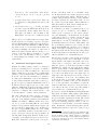
The following graphs compare the JAGS and Stan
(Unconstrained model) outputs for four selected crossstudent parameters. The output is from coda and provides a traceplot on the left and a density plot for the
corresponding distribution on the right. Recall that
the principle di↵erence between JAGS and Stan is the
proposal distribution: JAGS uses a random walk proposal with a special distribution for the mixing parameters and Stan uses the Hamiltonian proposal. Also,
note that for Stan the complete run of 15,000 samples
is actually made up of a sort run of length 5,000 and
a longer run of length 10,000; hence there is often a
discontinuity at iteration 5,000.
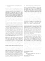
Although not strictly speaking a parameter, the deviance (twice the negative log likelihood) can easily
be monitored in JAGS. Stan does not o↵er a deviance
monitor, but instead monitors the log posterior, which
is similar. Both give an impression of how well the
model fits the data. Figure 4 shows the monitors for
the deviance or log posterior. This traceplot is nearly
ideal white noise, indicating good convergence for this
b is less than the heuristic threshvalue. The value of R
old of 1.1 for both chains, and the e↵ective sample size
is about 1/6 of the 45,000 total Monte Carlo observations.
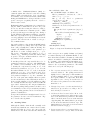
Figure 5 shows the grand mean of the log pause times
for the first component. The JAGS output (upper
row) shows a classic slow mixing pattern: the chains
are crossing but moving slowly across the support of
the parameter space. Thus, for JAGS even though
b
the chains have nearly reached pseudo-convergence (R
is just slightly greater than 1.1), the e↵ective sample
size is only 142 observations. A longer chain might
be needed for a good estimate of this parameter. The
Stan output (bottom row) looks much better, and the
e↵ective sample size is a respectable 3,680.
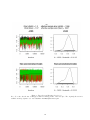
The Markov chains for ↵0,1 (the proportion of pause
times in the first component) have not yet reached
pseudo convergence, but they are close (a longer run
might get them there). Note the black chain often
ranges above the values in the red and green chains
in the JAGS run (upper row). This is an indication
that the chains may be stuck in di↵erent modes; the
Figure 4: Deviance (JAGS) and Log Posterior (Stan) plots
Note: To reduce the file size of this paper, this is a bitmap picture of the traceplot. The original pdf version is
available at http://pluto.coe.fsu.edu/mcmc-hierMM/DeviancePlots.pdf.
12
Figure 5: Traceplots and Density plots for µ0,1
Note: To reduce the file size of this paper, this is a bitmap picture of the traceplot. The original pdf version is
available at http://pluto.coe.fsu.edu/mcmc-hierMM/mu0Plots.pdf.
13
Figure 6: Traceplots and Density plots for ↵0,1
Note: To reduce the file size of this paper, this is a bitmap picture of the traceplot. The original pdf version is
available at http://pluto.coe.fsu.edu/mcmc-hierMM/alpha0Plots.pdf.
14
shoulder on the density plot also points towards multiple modes. The plot for Stan looks even worse, after
iteration 5,000 (i.e., after the chain was restarted), the
red chain has moved into the lower end of the support
of the distribution. This gives a large shoulder in the
corresponding density plot.
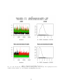
The chains for the variance of the log precisions for the
first component, 0,1 (Figure 7), are far from pseudob = 1.73. In the JAGS chains (top
convergence with R
row) the black chain seems to prefer much smaller values for this parameter. In the Stan output, the green
chain seems to be restricted to the smaller values in
both the first and second run. However, between the
first and second run the black and red chains swap
places. Clearly this is the weakest spot in the model,
and perhaps a reparameterization here would help.
Looking at Figures 6 and 7 together, a pattern
emerges. There seems to be (at least) two distinct
modes. One mode (black chain JAGS, green chain in
Stan) has higher value for ↵0,1 and a lower value for
0,1 , and the other one has the reverse pattern. This
is an advantage of the MCMC approach over an EM
approach. In particular, if the EM algorithm was only
run once from a single starting point, the existence of
the other mode might never be discovered.
4.5
Data Point Labeling
For some applications, the analysis can stop after estimating the parameters for the students units, ⇡ i , µi
and ⌧ i (or i as desired). In other applications it is
interesting to assign the individual pauses to components, that is, to assign values to Zi,j .
When ⇡ i , µi and i are known, it is simple to calculate
(c,r)
(c,r)
(c,r)
pi,j,k = Pr(Zi,j = k). Let ⇡ i , µi
and i
be
the draws of the Level 1 parameters from Cycle r of
Chain c (after the data have been sorted to identify
the components). Now define,
(c,r)
(c,r)
qi,j,k = ⇡i,k
(c,r)
and set Qi,j
=
PK
(
Yi,j
(c,r)
k=1 qi,j,k .
(c,r)
µi,k
(c,r)
i,k
),
(17)
The distribution for Zi,j
(c,r)
(c,r)
(c,r)
for MCMC draw (c, r) is then pi,j,k = qi,j,k /Qi,j .
The MCMC estimate for pi,j,k is just the aver(c,r)
age over all the MCMC draws of pi,j,k , that is
PC PR
(c,r)
1
c=1
r=1 pi,j,k .
CR
If desired, Zi,j can be estimated as the maximum over
k of pi,j,k , but for most purposes simply looking at the
probability distribution pi,j provides an adequate, if
not better summary of the available information about
the component from which Yi,j was drawn.
15
4.6
Additional Level 2 Units (students)
In the pause time application, the goal is to be able
to estimate fairly quickly the student-level parameters
for a new student working on the same essay. As the
MCMC run is time consuming, a fast method for analyzing data from new student would be useful.
One approach would be to simply treat Equations 2,
3 and 4 as prior distributions, plugging in the point
estimates for the cross-student parameters as hyperparameters, and find the posterior mode of the observations from the new data. There are two problems
with this approach. First, the this method ignores any
remaining uncertainty about the cross-student parameters. Second, the existing mixture fitting software
packages (FlexMix and mixtools) do not provide any
way to input the prior information.
A better approach is to do an additional MCMC run,
using the posterior distributions for the cross-student
parameters from the previous run as priors from the
previous run (Mislevy et al., 1999). If the hyperparameters for the cross-student priors are passed to
the MCMC sampler as data, then the same JAGS or
Stan model can be reused for additional student pause
records. Note that in addition to the MCMC code
Stan provides a function that will find the maximum
of the posterior. Even if MCMC is used at this step,
the number of Level 2 units, I, will be smaller and the
chains will reach pseudo-convergence more quickly.
If the number of students, I, is large in the original
sample (as is true in the original data set), then a
sample of students can be used in the initial model
calibration, and student-level parameters for the others can be estimated later using this method. In particular, there seems to be a paradox estimating models using large data sets with MCMC. The larger the
data, the slower the run. This is not just because
each data point needs to be visited within each cycle
of each Markov chain. It appears, especially with hierarchical models, that more Level 2 units cause the
chain to have higher autocorrelation, meaning larger
runs are needed to achieve acceptable Monte Carlo error. For the student keystroke logs, the “initial data”
used for calibration was a sample of 100 essays from
the complete collection. There is a obvious trade-o↵
between working with smaller data sets and being able
to estimate rare events: I = 100 seemed like a good
compromise.
5
Model Selection
A big question in hierarchical mixture modeling is
“What is the optimal number of components, K?”
Although there is a way to add a prior distribution
Figure 7: Traceplots and Density plots for 0,1
Note: To reduce the file size of this paper, this is a bitmap picture of the traceplot. The original pdf version is
available at http://pluto.coe.fsu.edu/mcmc-hierMM/gamma0Plots.pdf.
16
over K and learn this as part of the MCMC process, it is quite tricky and the number of parameters
varies for di↵erent values of K. (Geyer, 2011, describes
the Metropolis-Hastings-Green algorithm which is required for variable dimension parameter spaces). In
practice, analysts often believe that the optimal value
of K is small (less than 5), so the easiest way to determine a value of K is to fit separate models for
K = 2, 3, 4, . . . and compare the fit of the models.
Gelman et al. (2013) advocate using a new measure of
model selection called WAIC. WAIC makes two substitutions in the definition of AIC above. First, it uses
D(⌦) in place of D(⌦). Second, it uses a new way of
calculating the dimensionality of the model. There are
two possibilities:
Note that increasing K should always improve the fit
of the model, even if the extra component is just used
to trivially fit one additional data point. Consequently,
analysts use penalized measures of model fit, such as
AIC to chose among the models.
(21)
Chapter 7 of Gelman et al. (2013) gives a good
overview of the various information criteria, so the
current section will provide only brief definitions. Recall Equation 5 that described the log likelihood of
the complete data Y as a function of the complete
parameter ⌦. By convention, the deviance is twice
the negative log likelihood: D(⌦) = 2L(Y|⌦). The
lower the deviance, the better the fit of the data to the
model, evaluated at that parameter. As students are
independent given the cross-student parameters, and
pause times are independent given the student-level
e for some value of the parameters
parameters, D(⌦),
e
⌦ can be written as a sum:
e =
D(⌦)
Ji
I X
X
i=1 j=1
e ,
log Qi,j (⌦)
(18)
e is the likelihood of data point Yi,j , that
where Qi,j (⌦)
is:
k
X
Yi,j µ
g
i,k
e =
Qi,j (⌦)
⇡
g
).
(19)
i,k (
g
i,k
k=1
Note that the cross-student parameters drop out of
these calculations.
The Akaike information criterion (AIC) takes the deviance as a measure of model fit and penalizes it for
b be the
the number of parameters in the model. Let ⌦
maximum likelihood estimate of the parameter. Then
AIC is defined as:
b +2⇤m
AIC = D(⌦)
(20)
where m = K(2IK + 4) + (K 1)(I + 1) + 1 is the
number of free parameters in the model. Note that
the MCMC run does not provide a maximum likelihood estimate. A pseudo-AIC can be computed by
substituting ⌦, the posterior mean of the parameters
⌦. Note that ⌦ must be calculated after the parameters in each MCMC cycle are permuted to identify the
components.
17
pWAIC1 = 2
Ji
I X
X
(log E[Qi,j (⌦)]
Ji
I X
X
Var(Qi,j (⌦)) .
E[log Qi, j(⌦)]) ,
i=1 j=1
pWAIC2 = 2
(22)
i=1 j=1
The expectation and variance are theoretically defined
over the posterior distribution and are approximated
using the MCMC sample. The final expression for
WAIC is:
WAIC = D(⌦) + 2 ⇤ mWAIC .
(23)
For all of the model fit statistics discussed here: AIC,
WAIC1 and WAIC2 , the model with the lowest value
is the best. One way to chose the best value of K is to
calculate all of these statistics for multiple values of K
and choose the value of K which has the lowest value
for all 5 statistics. Hopefully, all of the statistics will
point at the same model. If there is not true, that is
often evidence that the fit of two di↵erent models is
too close to call.
In the 27 runs using the data from known values of K,
simply using the lowest WAIC value was not sufficient
to recover the model. As the Markov chains have not
yet reached pseudo-convergence, the WAIC values may
not be correct, but there was fairly close agreement on
both WAIC1 and WAIC2 for both the JAGS and Stan
(unconstrained) models. However, the values of both
WAIC1 and WAIC2 were also fairly close for all values
of K 0 (number of estimated components). For example
when K = 2 the WAIC1 value was 1132, 1132 and
1135 for K 0 = 2, 3 and 4 respectively when estimated
with JAGS and 1132, 1131, and 1132 when estimated
with Stan. The results for WAIC2 were similar. It
appears as if the common practice of just picking the
best value of WAIC to determine K is not sufficient.
In particular, it may be possible to approximate the
data quite well with a model which has an incorrect
value of K.
6
Conclusions
The procedure described above is realized as code in
R, Stan and JAGS and available for free at http://
pluto.coe.fsu.edu/mcmc-hierMM/. Also available,
are the simulated data for trying out the models.
These scripts contain the functions necessary to automatically set starting parameters for these problems,
identify the components, and to calculate WAIC model
fit statistics.
The scripts seem to work fairly well for a small number
of students units (5 I 10). With this sample size,
although JAGS has the faster run time, Stan has a
larger e↵ective sample size. Hamiltonian Monte Carlo.
With large sample sizes I = 100, Ji ⇡ 100 even the
HMC has high autocorrelation and both JAGS and
Stan are extremely slow. Here the ability of JAGS to
allow the user to selectively monitor parameters and
to extend the chains without starting over allows for
better memory management.
The code supplied at the web site solves two key technical problems: the post-run sorting of the mixture
components (Früthwirth-Schnatter, 2001) and the calculation of the WAIC model-fit indexes. Hopefully,
this code will be useful for somebody working on a
similar application.
The model proposed in this paper has two problems,
even with data simulated according to the model. The
first is the slow mixing. This appears to be a problem with multiple modes, and indicates some possible
non-identifiability in the model specifications. Thus,
further work is needed on the form of the model. The
second problem is that the WAIC test does not appear to be sensitive enough to recover the number of
components in the model. As the original purpose of
moving to the hierarchical mixture model was to discover if there were rare components that could not be
detected in the single-level hierarchical model, the current model does not appear to be a good approach for
that purpose.
In particular, returning to the original application of
fitting mixture models to student pauses while writing,
the hierarchical part of the model seems to be creating as many problems as it solves. It is not clearly
better than fitting the non-hierarchical mixture model
individually to each student. Another problem it has
for this application is the assumption that each pause
is independent. This does not correspond with what
is known about the writing process: typically writers spend long bursts of activities simply doing transcription (i.e., typing) and only rarely pause for higher
level processing (e.g., spelling, grammar, word choice,
planning, etc). In particular, rather than getting this
model to work for this application, it may be better to
look at hidden Markov models for individual student
writings.2
The slow mixing of the hierarchical mixture model
2
Gary Feng and Paul Deane, private communication.
18
for large data sets indicates that there may be additional transformation of this model that are necessary
to make it work properly. Hopefully, the publication of
the source code will allow other to explore this model
more fully.
References
Almond, R. G., Deane, P., Quinlan, T., Wagner,
M., & Sydorenko, T. (2012). A preliminary analysis of keystroke log data from a
timed writing task (Research Report No.
RR-12-23). Educational Testing Service. Retrieved from http://www.ets.org/research/
policy research reports/publications/
report/2012/jgdg
Benaglia, T., Chauveau, D., Hunter, D. R., & Young,
D. (2009). mixtools: An R package for analyzing finite mixture models. Journal of Statistical Software, 32 (6), 1–29. Retrieved from
http://www.jstatsoft.org/v32/i06/
Brooks, S., Gelman, A., Jones, G. L., & Meng, X.
(Eds.). (2011). Handbook of markov chain monte
carlo. CRC Press.
Deane, P. (2012). Rethinking K-12 writing assessment.
In N. Elliot & L. Perelman (Eds.), Writing assessment in the 21st century. essays in honor of
Edward M. white (pp. 87–100). Hampton Press.
Früthwirth-Schnatter, S. (2001). Markov chain
Monte Carlo estimation of classical and dynamic
switching and mixture models. Journal of the
American Statistical Association, 96 (453), 194–
209.
Gelman, A., Carlin, J. B., Stern, H. S., Dunson, D. B.,
Vehtari, A., & Rubin, D. B. (2013). Bayesian
data analysis (3rd ed.). Chapman and Hall. (The
third edition is revised and expanded and has
material that the earlier editions lack.)
Gelman, A., & Shirley, K. (2011). Inference from
simulations and monitoring convergence. In
S. Brooks, A. Gelman, G. L. Jones, & X. Meng
(Eds.), Handbook of markov chain monte carlo
(pp. 163–174). CRC Press.
Geyer, C. J.
(2011).
Introduction to Markov
chain Monte Carlo. In S. Brooks, A. Gelman,
G. L. Jones, & X. Meng (Eds.), Handbook of
markov chain monte carlo (pp. 3–48). CRC
Press.
Gruen, B., & Leisch, F. (2008). FlexMix version
2: Finite mixtures with concomitant variables
and varying and constant parameters. Journal
of Statistical Software, 28 (4), 1–35. Retrieved
from http://www.jstatsoft.org/v28/i04/
Li, T. (2013). A Bayesian hierarchical mixture approach to model timing data with application to
writing assessment (Unpublished master’s thesis). Florida State University.
McLachlan, G., & Krishnan, T. (2008). The EM algorithm and extensions (2nd ed.). Wiley.
McLachlan, G., & Peel, D. (2000). Finite mixture
models. Wiley.
Mislevy, R. J., Almond, R. G., Yan, D., & Steinberg, L. S. (1999). Bayes nets in educational
assessment: Where the numbers come from. In
K. B. Laskey & H. Prade (Eds.), Uncertainty in
artificial intelligence ’99 (p. 437-446). MorganKaufmann.
Neal, R. M. (2011). MCMC using Hamiltonian dynamics. In MCMCHandbook (Ed.), (pp. 113–162).
Plummer, M. (2012, May). JAGS version 3.2.0
user manual (3.2.0 ed.) [Computer software
manual]. Retrieved from http://mcmc-jags
.sourceforge.net/
Plummer, M., Best, N., Cowles, K., & Vines, K.
(2006). Coda: Convergence diagnosis and output analysis for mcmc. R News, 6 (1), 7–11.
Retrieved from http://CRAN.R-project.org/
doc/Rnews/
R Core Team. (2014). R: A language and environment for statistical computing [Computer software manual]. Vienna, Austria. Retrieved from
http://www.R-project.org/
Stan Development Team. (2013). Stan: A C++ library
for probability and sampling (Version 2.2.0 ed.)
[Computer software manual]. Retrieved from
http://mc-stan.org/
Thomas, A., O’Hara, B., Ligges, U., & Sturtz, S.
(2006). Making BUGS open. R News, 6 , 12-17.
Retrieved from http://www.rni.helsinki.fi/
~boh/publications/Rnews2006-1.pdf
Thomas, A., Spiegelhalter, D. J., & Gilks, W. R.
(1992).
BUGS: A program to perform
Bayesian inference using Gibbs sampling. In
J. M. Bernardo, J. O. Berger, A. P. Dawid, &
A. F. M. Smith (Eds.), Bayesian statistics 4. (pp.
837–842). Clarendon Press.
Acknowledgments
Tingxuan Li wrote the first version of much of the
R code as part of her Master’s thesis. Paul Deane
and Gary Feng of Educational Testing Service have
been collaborators on the essay keystroke log analysis
work which is the inspiration for the present research.
Various members of the JAGS and Stan users groups
and development teams have been helpful in answering emails and postings related to these models, and
Kathy Laskey and several anonymous reviewers have
given me useful feedback (to which I should have paid
closer attention) on the draft of this paper.
19