Download CHEMICAL MOVEMENT IN LAYERED SOILS, CMLS

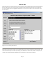
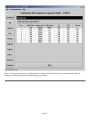
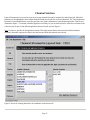
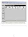
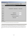
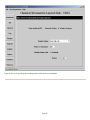
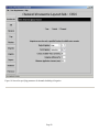
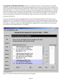
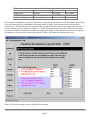
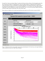
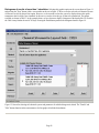
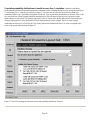
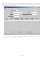
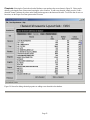
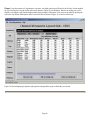
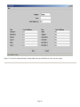
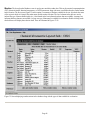
CHEMICAL MOVEMENT IN LAYERED SOILS, CMLS
Java Web Start Version
By
D.L. Nofziger and Jinquan Wu
Department of Plant and Soil Sciences
Oklahoma State University
Stillwater, OK 74078
Revised May, 2005
PURPOSE OF PROGRAM
CMLS (Nofziger and Hornsby, 1986, 1987) was written to provide a tool for managing agricultural chemicals. The interactive
program was written in a manner which is easy to use. The software includes graphical output to aid in understanding and
comparing simulated movement and fate of chemicals. The model was designed to use soil and chemical parameters which are
readily available. The model is being used widely, especially in educational settings. Recently, it has been compared with
experimental measurements and with other models with good results (Pennell et al., 1990; Nofziger et al., 1994). Because the
model requires only basic soil properties which are readily available or easily estimated, the model has been used for
evaluating the impact of pesticides on large areas. A batch program using the computational algorithms of CMLS was
developed and interfaced with geographic information systems (Zhang et al., 1990; Ma, 1993). This batch program facilitated
simulation for many soils and chemicals with minimal user effort.
CMLS was originally written for MS-DOS computers in the early days of interactive software. It was revised in 1994 to
include (1) functions for estimating daily infiltration and evapotranspiration from daily weather records, (2) irrigation routines,
(3) a stochastic weather generator, WGEN, (4) Monte Carlo simulation using different weather sequences at a particular site,
(5) an improved user interface, (6) expanded graphics options and increased resolution, and (7) database management features.
CMLS94 was also written for MS-DOS computers. We soon realized that a batch version of the software was needed to enable
users to simulate movement of many chemicals through many soils with little user input and to store output in files for later
processing. That software, called CMLS98B, includes the computational algorithms used in CMLS94 without the interactive
features used to define soil - chemical - management systems, to select and display graphs and reports of simulated results, to
manage databases, and to display on-line help. CMLS98B was written in standard C and can be used on any platform
supporting standard C.
With the advent and popularity of the Windows operating system, users requested and expected a version of CMLS with a
graphical user interface. This manual describes CMLS2000, a version of CMLS designed with a graphical user interface and
enhanced capabilities.
Page 1
COMPUTER PLATFORMS AND SOFTWARE INSTALLATION
The software is written in Java and runs as a Java Web Start application. The Java run-time package and Web Start software
are available free of charge from Sun Microsystems, Inc. The program was developed and tested on various Windows
platforms as well as on Linux and MacOS X. We recommend 256 MB or more of Random Access Memory. Approximately 40
MB of disk space is required.
Before a Java Web Start program can be used on a computer, the supporting software must be installed. This is needed only 1
time per computer no matter how many different applications use it. Sun Microsystems Inc provides this package free of
charge at http://java.sun.com/products or it can be downloaded here. If this is the first time you are using it, just download the
file from the site above. Follow the instructions given there for installations. I recommend that you accept the default values
proposed in the install process.
After you have installed the Java Runtime Environment on your computer (as described in the preceding paragraph), click
here to download and start the program. If you use the program more than one time, you will be given the option of storing an
icon for the program on your local computer. You can then start the program without being connected to the internet.
Page 2
MODEL PROCESSES AND ASSUMPTIONS
In this section, the conceptual and mathematical framework of CMLS98B is presented. As that is done, we have attempted to
identify major simplifying assumptions which were used. We strongly recommend that you evaluate the appropriateness of
these assumptions for the systems of interest to you. We have found them acceptable for many problems, but you must keep
them in mind when interpreting results of this model just as you must do when using any model. Comparisons of transport
models which include CMLS have been published by Pennell et al.(1992) and Bergström and Jarvis (1994).
Chemical Movement: The basic computational part of CMLS94 and CMLS98B is the same as that used in CMLS
(Nofziger and Hornsby, 1986). A summary of the model is presented here so changes and assumptions can be noted and
evaluated.
The model is a modification of the work of Rao, Davidson, and Hammond (1976). It estimates the depth of the center of mass
of a non-polar chemical as a function of time after application. It also calculates the amount of chemical in the soil profile as a
function of time.
The model assumes that chemicals move only in the liquid phase in response to soil-water movement. All of the water in the
soil is active in the flow process. Water already in the profile is pushed ahead of the inflowing water in a piston-like manner.
Water is lost from the root zone by evapotranspiration and deep percolation. Movement of the chemical is retarded by its
sorption on the solid soil surfaces. The linear, reversible, equilibrium model is used to describe this sorption process.
Dispersion of the chemical is ignored. The soil profile can be divided into 20 layers with different properties in each layer. Soil
and chemical properties are uniform within a layer.
Since the chemical moves with soil water, the change in depth of the chemical depends upon the amount of water passing the
chemical. If DC(t) represents the chemical depth at time t and q represents the amount of water passing that depth during time
dt, the depth of chemical at time t+dt is given by
DC (t + dt) = DC (t) +
q
RθFC
(1)
where θFC is the volumetric water content of the soil at "field capacity" and R is the retardation factor for the chemical in the
current layer of the soil. The retardation factor is given by
R = 1+
ρK d
θFC
(2)
where ρ is the bulk density of the soil and Kd is the partition coefficient or linear sorption coefficient of the chemical in the
soil. Equation 2 assumes the sorption process can be described by the linear, reversible, equilibrium sorption model. The
partition coefficient, Kd, depends upon the soil and chemical properties. However for many soils and organic chemicals it can
be estimated from the organic carbon partition coefficient, KOC, using the equation
K d = K OCOC
(3)
where OC is the organic carbon content of the soil (Hamaker and Thompson, 1972; Karickhoff, 1981, 1984). This equation is
used in the model to estimate Kd for each layer of each soil. However, the user can enter a specific Kd for each layer if that is
Page 3
known.
ASSUMPTIONS IN CHEMICAL MOVEMENT
1.
2.
3.
4.
Chemicals move only in liquid phase.
Dispersion of the chemical can be ignored.
Soil and chemical properties are uniform within a soil layer.
All water in the profile takes part in the flow process. Water already in the soil profile is pushed ahead of infiltrating
water in a piston-like manner.
5. The sorption process can be described by the linear, reversible, equilibrium model.
Water Balance: CMLS98B evaluates the depth of the chemical using equation 1 with dt equal to one day. This means
that q, the amount of water moving downward past the current location of the chemical, must be estimated each day. In this
model q is equal to the amount of water entering the soil surface minus the quantity of water which is stored in the soil profile
above the chemical. The quantity of water stored depends upon the amount of water entering the soil surface, the wetness of
the soil before infiltration and the capacity of the soil to store water, and the current chemical depth. Daily infiltration amounts
are read from a file or are estimated from weather data as described on the following pages. At the beginning of simulation, the
soil is assumed to be at field capacity at all depths. Each day the water content in the root zone is reduced by the amount of
evapotranspiration on that day. Thus the water content throughout the root zone can be determined. (The soil water content is
never reduced below the water content at permanent wilting point.) Knowledge of the water content distribution enables one to
calculate the water storage capacity above the current chemical depth. Hence q can be determined. Thus, for each day
simulated (1) the water content in the root zone is adjusted for evapotranspiration, (2) the water content in the soil is adjusted
for infiltration, (3) the flux of water passing the chemical is determined, (4) the new depth of chemical is calculated, and (5)
the amount of chemical remaining in the soil is calculated. The following paragraphs present the details of these calculations.
In those paragraphs the soil is made up of layers entered by the user and additional layers with bottoms at the root zone depth
and at the current depth of the chemical.
Step 1. Adjustment for Evapotranspiration: CMLS98B assumes water is removed from the root zone to meet daily
evapotranspiration demands. The water content of the root zone never decreases below the water content at permanent wilting
point. Evapotranspiration is partitioned between layers in the root zone such that each layer looses water in proportion to the
amount of water available for plant growth which is stored in that layer. The water stored in a layer j at time t is given by
WS( j) = T( j)[θ( j,t) − θPWP ( j)]
(4)
where WS(j) is the water stored, T(j) is the thickness of the layer, θ(j,t) is the volumetric water content of the layer, and θPWP(j)
is the water content of layer j at permanent wilting point. The total water stored in the root zone is
n
WS TOTAL = ∑ WS( j)
(5)
j=1
where n is the number of layers in the root zone. The water content after evapotranspiration θ’(j,t) is
θ′( j,t) = θ( j,t) −
ET • WS( j)
WS TOTAL T( j)
(6)
where ET is the evapotranspiration on the current day. If θ’(j, t) calculated from equation 6 is less than θPWP(j), θ’(j, t)is set
equal to θPWP(j).
Page 4
ASSUMPTIONS IN STEP 1
1. The amount of water removed by evapotranspiration from each layer of the root zone is proportional to the amount of
available water in that layer.
2. The water content of the soil does not decrease below the permanent wilting point.
3. Water does not move upward from below the root zone. The chemical does not move upward anywhere in the profile.
Step 2. Adjust Water Content for Infiltration: Water content in the soil root zone is adjusted for infiltration by filling
consecutive layers of the profile to field capacity until the entire root zone is recharged or until the infiltrating water has been
stored. The amount of water required to recharge a layer to field capacity (or the soil-water deficit for the layer) is given by
swd( j) = T( j)[θFC − θ′( j,t)]
(7)
If I(j,t+dt) represents the amount of water infiltrating into layer j between time t and time t + dt, then the amount of water
entering layer j+1 is given by
I( j + 1,t + dt) = I( j,t + dt) − swd( j)
(8)
If I(j+1, t+dt) is greater than zero then θ(j,t+dt) = θFC(j) and equations 7 and 8 are applied to the next layer in the root zone. If
I(j+1, t+dt) in equation 8 is less than zero, then I(j+1, t+dt) = 0 and
θ( j,t + dt) = θ′( j,t) +
I( j,t + dt)
T( j)
(9)
For layers below the root zone, the water content is equal to the field capacity at all times. Thus water passing the root zone
depth passes all depths below that.
ASSUMPTIONS IN STEP 2
1. Infiltrating water recharges one layer of soil to field capacity before water moves deeper into soil.
2. Infiltrating water redistributes instantly to field capacity.
3. Water content of soil below the root zone is never less than field capacity.
Step 3. Calculate Flux Passing Chemical: The flux of water, q, passing the depth of the chemical is equal to the flux of water
passing the root zone depth if the chemical depth exceeds the root zone depth. If the chemical depth is less than the root zone
depth, the flux, q, is equal to I(JC, t+dt) given in equation 8 where JC is the index of the layer with bottom at the chemical
depth. If the infiltrating water is stored before reaching the bottom of layer JC, q is zero.
Step 4. Calculate New Chemical Depth: The depth of chemical at time t+dt is calculated using equation 1 for each soil layer. If
q equals zero, DC(t+dt) = DC(t). NOTE: If q obtained in step 3 is larger than needed to move the chemical to the bottom of the
next layer, the excess must be calculated and used in equation 1 with appropriate properties of succeeding layers.
Page 5
Step 5. Degradation: Degradation of the chemical in the soil is assumed to be described by first-order processes. The amount of
chemical remaining in the soil at time t+dt is given by
M(t + dt) = M(t)0.5 dt / half −life(t)
(10)
where M(t) and M(t+dt) represent the amount at times t and t+dt, respectively, and half-life(t) is the degradation half-life of the
chemical at time t.
By default, the half-life is taken as a constant over all times. However, CMLS98B is capable of adjusting the degradation halflife for temperature changes. The half-life at time t and the depth of the pesticide mass center where the soil temperature is
Temp(t) is given by
⎡E ⎛
⎞⎤
1
1
−
half − life(t) = HREF exp ⎢ a ⎜
⎟⎥
⎣⎢ R ⎝ Temp(t) TempREF ⎠ ⎦⎥
(11)
Here HREF(j) is the reference half-life determined at the incubation temperature TempREF for layer j, Ea is the activation energy
of the degradation reaction, and R is a universal gas constant (0.008315 kJ mol-1 oK-1).
The soil temperature at the pesticide mass center at time t is predicted from observed surface soil temperature data using the
equation
⎛ t − t o Dc (t) π ⎞
Temp(t) = Temp ave + A o e −(Dc (t) / d) sin ⎜ 2π
−
− ⎟
365
d
2⎠
⎝
(12)
where Tempave and A0 are the annual mean and amplitude of daily average surface soil temperature, t0 is the time lag from the
starting date of simulation to the occurrence of the minimum temperature in a year, and d is the damping depth of annual
fluctuation.
CMLS98B uses dt equal to one day and selects j as the layer containing the chemical at time t. The damping depth d is
estimated from clay content of the solid particles, porosity, and an average water content of the composite soil (Wu and
Nofziger, 1998). The annual mean, amplitude, and time lag are evaluated through a least-square optimization procedure to
eliminate the noisy fluctuation, they can also be estimated from observed annual maximum and minimum temperatures (Wu
and Nofziger, 1998).
ASSUMPTIONS IN STEP 5
1. The degradation is a first-order process.
2. All chemical in the soil degrades at the rate determined by the location of the center of mass.
Page 6
Infiltration Estimation From Rainfall: CMLS requires daily infiltration amounts as described above. CMLS required the user to
estimate this daily infiltration and enter it into infiltration files. CMLS98B provides the user with the option of having the
system estimate infiltration from daily rainfall. The capability of estimating these amounts is useful for simulating movement
at many locations and for Monte Carlo simulations at a particular site. The USDA-SCS curve number technique (USDA-SCS,
1972; Haan et al, 1993) was incorporated for estimating infiltration. The amount of water, I, infiltrating a soil due to
precipitation, P, is given by
I=P−
(P − 0.2S)2
(P + 0.8S)
for P > 0.2S
I=P
(13)
for P ≤ 0.2S
where the retention parameter S is given by
⎡
WSTOTAL ⎤
S = SMAX ⎢1.0 −
⎥
WSMAX ⎦
⎣
(14)
WSTOTAL is the current amount of water stored in the root zone as given by equations 4 & 5. WSMAX is the maximum water
storage capacity of the root zone (obtained using equations 4 and 5 with θ(j,t) replaced by the saturated water content, θSAT).
SMAX is an estimate of the largest S for this soil and is estimated by the equation
SMAX =
1000
− 10
CNI
(15)
with
CNI =
4.2CNII
10 − 0.058CNII
(16)
where CNII is the "moisture condition II" curve number for the soil. CNII values are the normal tabulated curve numbers.
Equations 13 to 16 estimate infiltration in inches for precipitation in inches.
Page 7
Evapotranspiration Estimation: Four sources of daily evapotranspiration (ET) are currently supported in
CMLS98B. These are (1) actual ET values stored in a data file, (2) estimated ET using daily pan evaporation data, (3)
estimated ET using the SCS Blaney-Criddle equations with historical or generated weather data, and (4) estimated ET using
the FAO Blaney-Criddle method and historical or generated weather. Users can use other estimators outside of CMLS98B and
create "actual" ET files for use in this software. However, only the Blaney - Criddle estimators can be used for Monte Carlo
simulations. If you have other estimators you would like to have incorporated, contact the authors. (The methods used to
estimate infiltration and flux of water passing the current chemical depth make CMLS98B somewhat less sensitive than many
crop models to the distribution of daily evapotranspiration. In fact, CMLS98B is sensitive only to the total ET between
infiltration events. The distribution of ET during that time period has no effect on the predicted flux of water and chemical
leaching.)
The basic concept with all of the ET estimators is to determine a reference crop evapotranspiration value, ET0, and to relate
ET0 to ET for the crop of interest by means of time dependent crop coefficients, kCROP(t). That is
ET(t) = k CROP (t)ET0 (t)
(17)
Values of kCROP(t) are obtained by linear interpolation between tabulated kCROP(t') values where t' is time measured from the
date of planting.
For the pan evapotranspiration method, the reference crop evapotranspiration is given by
ET0 (t) = K • Pan(t)
(18)
where K is a pan constant and Pan(t) is the pan evaporation amount on day t.
In CMLS98B the SCS Blaney-Criddle estimate of ET0 is calculated by dividing the estimated monthly consumptive use by the
number of days in the month. Each day in the month then has the same ET0 value. The consumptive use, U, for the month is
obtained using the equation
U=K
TempF • p
100
(19)
where K is the consumptive use factor specified by the user, TempF is the mean monthly air temperature in degrees Fahrenheit,
and p is the mean monthly percentage of annual daytime hours (Jensen et al., 1990). A table of values of p as a function of
latitude from 0 to 64 degrees is built into the software. The mean temperature is taken as the mean of the high and low
temperatures for each day in the month. The value of U calculated in equation 19 has units of inches.
The reference crop evapotranspiration for the FAO Blaney-Criddle method is given by
ET0 = a + b • f
(20)
where a and b are constants for a particular site and
f = p[0.46TempC + 8.13]
(21)
Here p is the mean daily percent of annual daytime hours, and TempC is the mean air temperature in degrees Celsius (Jensen et
al., 1990). The mean temperature is taken as the mean of the high and low temperatures for each day in the month. ET0 in
Page 8
equation 20 has units of mm.
Weather Generating: CMLS98B incorporates the stochastic model for generating daily weather variables
developed by Richardson and Wright (1984). This software uses parameters derived from 10 or more years of daily weather
data at a site to generate daily rainfall, minimum and maximum temperatures, and radiation characteristic of the site. WGEN
enables one to examine the behavior of chemicals at a site which has only limited historical data. It is used to determine
probability distributions for chemical fate and transport at a particular site. Since future weather is not known at the site, the
model can be used to generate many independent sequences of weather data typical of that site. By simulating the movement
of the chemical for each weather sequence, probability distributions can be determined for soil - chemical - management
systems of interest.
The publication of Richardson and Wright (1984) includes a program for extracting the parameters needed to generate weather
from historical weather data.
Irrigation: The irrigation module is capable of applying water in two primary modes (in addition to using actual
irrigation stored in a data file). In the first case, irrigation is scheduled by the calendar. In this mode, called periodic, a
specified amount of water is applied at a specified time interval during the irrigation season. In the second case, irrigation is
scheduled by the available water remaining in the root zone. During the irrigation season, this demand mode of irrigation
applies water whenever the amount of available water in the root zone is decreased below some critical depletion level. The
amount of water to be applied is calculated by dividing the amount of water needed to return the root zone to field capacity by
the application efficiency. If this calculated amount of water needed is less than the minimum amount of water which can be
applied by the system, the minimum amount will be applied. For example, if 30 mm of water is needed to return the soil to
field capacity and the application efficiency is 75% and the minimum amount which can be applied is 35 mm, the amount of
water applied would be 40 mm (30 mm/0.75 = 40 mm which is larger than 35 mm minimum). If the application efficiency is
90%, 35 mm would be applied (30 mm/.90 = 33.3 mm which is less than the 35 mm minimum).
ASSUMPTION ABOUT IRRIGATION
1. All irrigation water infiltrates into the soil.
Page 9
SOFTWARE INTRODUCTION
Figure 1 shows the opening screen of CMLS. Along the left side of the screen are options needed to define soil-chemicalmanagement systems and to view the results in graphical and tabular forms. It also includes an option for managing the
databases used in CMLS so new soil, chemical, and weather data can be added or modified and saved in computer files for use
at a later date. The Preferences button allows the user to select units used in the displays and certain computational schemes
used in the software.
Soil and weather data are associated with different geographical regions of the world. The user selects the geographical region
of interest in this opening screen.
Figure 1. Introductory screen of CMLS2000. The geographical region of interest is selected here.
Page 10
Soil Selection
Figure 2 shows the screen used to select one or more soils of interest. Each geographical region of interest can be broken down
into areas. When the user selects the area of interest, available soils from that area are displayed in the list of available soils.
One or more available soils can be highlighted and added to the list of selected soils. In this case, three soils from the Caddo
area were selected.
Figure 2. Screen for selecting soils of interest.
At the bottom of the screen for selecting soils, is a button that can be used to view the soil properties of the selected soils. That
screen is illustrated in Figure 3. Here the organic carbon content, bulk density, volumetric water content at field capacity (FC),
volumetric water content at permanent wilting point (PWP), and porosity of each soil layer are displayed.
Page 11
Figure 3. Soil properties screen for viewing properties of selected soils. If more than one soil was selected, the soil to be
displayed is selected in the pull-down menu at the top of the screen.
Page 12
Chemical Selection
Figure 4 illustrates the screen used to select one to twenty chemicals that can be simulated for each selected soil. Individual
chemicals can be highlighted in the available chemical list and moved to the list of selected chemicals. The "Enter Application
Parameters" button should then be pressed to specify the date, depth, and amount of each chemical application. That screen is
illustrated in Figure 5. To simulate a chemical applied several times per year, the chemical can be selected several times on the
selection screen (Figure 4) and different application dates used on the screen in Figure 5.
Note: No units are specified for the application amount. This simply means that the units associated with the simulated
amounts in the model output are the same as the units assumed when these amounts were entered.
Figure 4. Screen for selecting chemicals to be simulated in each selected soil.
Page 13
Figure 5. This screen enables the user to define the application date, application depth, and application amount for each
selected chemical. The organic carbon partition coefficient, half-life, and critical concentration are displayed but cannot be
edited here.
Page 14
Crop Selection
The amount of water lost by evapotranspiration depends upon the crop growing in the field of interest and the season of the
year and the root depth of the crop. The software calculates potential evapotranspiration for a reference crop from weather
data. This amount is multiplied by a crop coefficient to obtain the potential evapotranspiration amount for each day of the
simulation. These parameters for a crop can be defined in the database option. Figure 6. illustrates the screen for selecting the
crop of interest. Root depth, and crop coefficient values can be edited in this screen but values are not saved permanently in the
database. Crop coefficients between dates listed are obtained by linear interpolation.
Figure 6. Screen for selecting crop being grown in the soil of interest and editing parameters associated with that crop.
Page 15
Weather
The Weather option (Figures 7 and 8) are used to define sources for daily rainfall and potential evapotranspiration data
required by CMLS. These daily amounts can be obtained in three ways. The first is from data files containing daily rainfall and
daily potential evapotranspiration (calculated outside of CMLS). The second is from daily weather files containing daily
rainfall and maximum and minimum temperatures along with the coordinates of the weather station. The third is by means of
the WGEN weather generator.
Figure 7 illustrates the screen for using historical weather. It indicates that the Fort Cobb station has data for 1948 to 1975.
That means that the application date specified in the chemical application parameter screen must be in this range or no
simulation is possible. Because the weather at a site has a large impact upon the depth of movement, CMLS enables the user to
easily simulate movement for applications in different years so the user can get insight into the variation expected due to
weather. To do that, the software, attempts to apply the chemical at the same day of year for all years available in the weather
file following the application date specified for the chemical. In this example, the chemicals were applied in 1972 so only 3 or
4 applications are possible (depending upon the number of days to be simulated). If the application date were in 1948, a total of
28 simulations would be possible. The number of simulations desired is specified on this screen as "Number of years".
Page 16
Figure 7. Screen for specifying historical weather stations to be used in the simulations.
Figure 8 illustrates the screen used when the weather generator is the source of weather data. Here the user selects the weather
station of interest, the number of simulations desired (that is, the number of years in which the chemical is applied) and
whether the computer should use a specific seed for the random number generator or just get a seed from the current value of
the computer clock. The results shown in this manual are based on using this weather station and 100 simulations as shown
here.
Page 17
Figure 8. Screen for specifying the weather generator as the source of weather data.
Page 18
Irrigation
Irrigation practices can have a large impact upon chemical leaching. CMLS supports two irrigation management systems. The
first is called periodic. In this method, a specified amount of water is applied at regular intervals during the irrigation season.
Figure 9 illustrates the screen used for periodic irrigation. The second type of irrigation is irrigation on demand. That is, the
amount of water stored in the root zone is calculated daily. During the irrigation season, when this amount of water reaches a
specified level, water is added to the soil to bring it back to field capacity. This input screen is shown in Figure 10. Irrigation
efficiency as used here refers to the ratio of the amount of applied water stored in the root zone to the amount of water applied
to the soil. In the illustration this is 70%, so if the root zone can store 21 mm of water at the time of irrigation, the system
would actually apply 30 mm (since 21 mm is 70% of 30 mm.)
Figure 9. Input screen for periodic irrigation.
Page 19
Figure 10. Screen for specifying parameters for demand scheduling of irrigation.
Page 20
Graphics
CMLS supports many different types of graphs as shown in Figure 11. The first type includes graphs of data from individual
simulations of soil-chemical-weather-management systems. The second summarizes groups of simulations using histograms.
The third summarizes groups of simulations as probability distributions. The final group ranks soil-chemical systems for their
potential to leach to groundwater.
Figure 11. Screen for selecting types of graphs to be displayed.
Page 21
Line graphs for individual simulations: Figures 12-14 illustrate the steps for creating line graphs for individual
simulations. Although this option shows data from individual simulations, many lines can be drawn on the same graph. These
can be for different soils, different chemicals, different crops, different weather, or different irrigation practices. The first step,
illustrated in Figure 12, is to select the soil-chemical systems to be shown on the graph. When more than one soil or chemical
is selected in the earlier screens, the system creates input parameters for each soil-chemical combination. These are listed in
Figure 12 as available systems. An abbreviated description of the system is found beside each number. Table 1 describes the
content of this description. Full details of the soil-chemical-weather system can be viewed, printed, or stored in a file by
pressing the Details button.
One or more soil-chemical systems are highlighted and moved to the Selected Systems window. Each selected system is
assigned a color. This is the default color used for lines from this system. The "Edit" button displays the partition coefficient
and half-life for each soil layer based on soil and chemical properties in the database. These parameters can be edited in this
screen if the user wants to use other values. When editing has been completed for all systems selected, the "Next" button is
pressed and the screen illustrated in Figure 13 is displayed.
Figure 12. Screen for selecting soil-chemical systems to be used in graphs.
Page 22
Table 1. Parameters listed in short description of soil-chemical systems in Graphics option.
Area
Soil Name
Crop
Chemical Name
Appl. Date
Appl. Depth
Appl. Amount
Rainfall Source
PET Source
Irrigation Type
Date Simulation Begins
Number of Simulations
The second step in defining the systems to be displayed is to choose the years of interest for each soil chemical system. If only
1 year is of interest, that year is highlighted in the column labeled "Available Years" and moved to the column labeled
"Desired Years". This selection process is repeated for each selected soil-chemical system. In the example shown in Figure 13,
all of the available years were selected by using the "<<" button. That means the system will draw 100 lines for each system
since that is the number of simulations specified in the weather panel (Figure 8). If the default color chosen by the computer is
not satisfactory, a new color can be chosen by pressing the "Choose Color" button at the bottom of the screen.
Figure 13. Screen for selecting years to be displayed for each system.
Page 23
Pressing "Next" on the screen shown in Figure 13 produces the final screen (shown in Figure 14) for this graphics option. Here
the user chooses the parameter to be displayed on the vertical axis and the parameter to be displayed on the horizontal axis
along with the number of days to be simulated for each chemical application. The example shown shows the depth of chemical
as a function of time after application for 365 days for all 100 simulations of 2,4-D Acid in the Cobb Loamy Sand and in the
Eufaula Sand. Clearly the chemical moves deeper in the Eufaula sand. Also, we can see the large range of depths predicted due
to different weather regimes all characteristic of the same weather station.
Many other types of graphs can be selected from the pull-down menu on this screen. These choices are given in Table 2.
Figure 14. Illustration of final screen in graphics option showing simulated depth of 2,4-D acid in two soils using 100 different
weather realizations for the site in Caddo County, Oklahoma.
Page 24
Table 2. Parameters that can be displayed on horizontal and vertical axes of line graphs.
Vertical Axis
•
•
•
•
•
•
•
•
•
•
•
•
•
•
•
•
•
Horizontal Axis
Time (including year of application)
Time after Application
Depth of Chemical
Amount of Chemical (linear scale)
Amount of Chemical (logarithmic scale)
Daily Rainfall
Cumulative Rainfall
Daily Evapotranspiration
Cumulative Evapotranspiration
Daily Irrigation
Cumulative Irrigation
Daily Infiltration
Cumulative Infiltration
Daily Drainage Below Root Zone
Cumulative Drainage Below Root Zone
Daily Flux Density Passing Chemical
Cumulative Flux Density Passing
Chemical
•
•
•
•
•
•
•
•
•
•
•
Page 25
Time (including year of application)
Time after Application
Depth of Chemical
Amount of Chemical (linear scale)
Amount of Chemical (logarithmic scale)
Cumulative Rainfall
Cumulative Evapotranspiration
Cumulative Irrigation
Cumulative Infiltration
Cumulative Drainage Below Root Zone
Cumulative Flux Density Passing
Chemical
Histograms of results of more than 1 simulation: Selecting this graphics option on the screen shown in Figure 11
and pressing the "Next" button yields a screen similar to the one in Figure 15. Here we need to select the soil-chemical system
of interest as we did for the previous option. However, we do not need to select the years to be displayed since this option
summarizes data for all the years simulated. In this case we need to select the type of data to be summarized. The options
available are shown in Table 3. In the example shown, we have chosen to display a histogram of the depth of the 2,4-D acid in
the Cobb Loamy Sand at the end of 365 days. Pressing the Finish button produces the histogram shown in Figure 16.
Figure 15. Screen for selecting soil-chemical systems and parameters for which a histogram is desired. The "Details" and
"Edit" buttons function in the same manner as for line graphs of individual simulations.
Page 26
Figure 16. Histogram showing the distribution of the simulated depth of 2,4-D acid 365 days after application in the Cobb
Loamy Sand soil based on 100 different weather realizations for the site in Caddo County, Oklahoma.
Page 27
Table 3. Types of histograms that can be selected.
Distribution of
• Depths at a specified time after application
• Depths at a specified amount of chemical remaining in profile
• Depths at a specified cumulative infiltration
• Depths at a specified cumulative drainage
• Depths at a specified cumulative flux density passing chemical
• Amounts of chemical (linear scale) passing a specified depth
• Amounts of chemical (logarithmic scale) passing a specified depth
• Amounts of chemical (linear scale) at a specified time after application
• Amounts of chemical (logarithmic scale) at a specified time after application
• Amounts of chemical (linear scale) at a specified cumulative infiltration
• Amounts of chemical (logarithmic scale) at a specified cumulative infiltration
• Amounts of chemical (linear scale) at a specified cumulative drainage
• Amounts of chemical (logarithmic scale) at a specified cumulative drainage
• Amounts of chemical (linear scale) at a specified cumulative flux density passing chemical
• Amounts of chemical (logarithmic scale) at a specified cumulative flux density passing
chemical
• Times to reach a specified depth
• Times to reach a specified amount remaining
• Times to reach a specified cumulative infiltration
• Times to reach a specified cumulative drainage
• Times to reach a specified cumulative flux density passing chemical
• Cumulative infiltration at a specified time after application
• Cumulative infiltration required to move chemical to specified depth
• Cumulative infiltration corresponding to a specified amount of chemical remaining
• Cumulative infiltration resulting in specified cumulative drainage
• Cumulative infiltration resulting in specified cumulative flux density passing chemical
• Cumulative drainage at a specified time after application
• Cumulative drainage corresponding to movement to a specified depth
• Cumulative drainage corresponding to a specified amount remaining
• Cumulative drainage resulting from a specified amount of infiltration
• Cumulative drainage corresponding to a specified cumulative flux density passing chemical
Page 28
Cumulative probability distributions of results for more than 1 simulation: Cumulative probability
distributions are often more useful than histograms to summarize results. Choosing this option on the screen shown in Figure
11 and pressing "Next" yields the screen shown in Figure 17. Here the user can select the soil-chemical systems to be
summarized and the type of probability distribution to be drawn. Types of probability distributions are shown in Table 4. The
user can also choose to draw separate probability distributions for each soil-chemical system or they can create a single
distribution for several systems. The combined approach is often of interest when the the different soils selected represent
different pedon properties of the soil found in the same management unit. In this example, Figure 18 shows separate
distributions are drawn for 2,4-D acid in the Cobb Loamy Sand and the Eufaula Sand soils. Line colors correspond to the
colors of the system numbers shown in Figure 17.
Figure 17. Screen for selecting soil-chemical systems and probability distribution of interest.
Page 29
Figure 18. Probability of exceeding different depths of 2,4-D acid 365 days after application in the Cobb Loamy Sand (red
line) and Eufaula Sand (purple line) soils based on 100 different weather realizations for the site in Caddo County,
Oklahoma.
Page 30
Table 3. Types of probability distributions that can be selected.
Probability of exceeding different
• Depths at a specified time after application
• Depths at a specified amount of chemical remaining in profile
• Depths at a specified cumulative infiltration
• Depths at a specified cumulative drainage
• Depths at a specified cumulative flux density passing chemical
• Amounts of chemical (linear scale) passing a specified depth
• Amounts of chemical (logarithmic scale) passing a specified depth
• Amounts of chemical (linear scale) at a specified time after application
• Amounts of chemical (logarithmic scale) at a specified time after application
• Amounts of chemical (linear scale) at a specified cumulative infiltration
• Amounts of chemical (logarithmic scale) at a specified cumulative infiltration
• Amounts of chemical (linear scale) at a specified cumulative drainage
• Amounts of chemical (logarithmic scale) at a specified cumulative drainage
• Amounts of chemical (linear scale) at a specified cumulative flux density passing chemical
• Amounts of chemical (logarithmic scale) at a specified cumulative flux density passing
chemical
• Times to reach a specified depth
• Times to reach a specified amount remaining
• Times to reach a specified cumulative infiltration
• Times to reach a specified cumulative drainage
• Times to reach a specified cumulative flux density passing chemical
• Cumulative infiltration at a specified time after application
• Cumulative infiltration required to move chemical to specified depth
• Cumulative infiltration corresponding to a specified amount of chemical remaining
• Cumulative infiltration resulting in specified cumulative drainage
• Cumulative infiltration resulting in specified cumulative flux density passing chemical
• Cumulative drainage at a specified time after application
• Cumulative drainage corresponding to movement to a specified depth
• Cumulative drainage corresponding to a specified amount remaining
• Cumulative drainage resulting from a specified amount of infiltration
• Cumulative drainage corresponding to a specified cumulative flux density passing chemical
Page 31
Reports
This option provides model output in tabular form. These tables can be viewed on the screen, printed on a printer, and saved in
text files for use in other programs. The steps involved are similar to those of graphics. The user must first select the type of
report desired from the screen shown in Figure 19. If "Selected parameters as a function of time" is chosen, the report will
contain detailed data on each simulation selected for each day simulated. If "Tabular summaries of more than one simulation",
the report will contain information about the collection of simulations.
Figure 19. Introductory screen for all reports. The user uses this screen to select the type of report desired and then presses the
"Next" button.
Page 32
Selected parameters as a function of time: To make this report, the user must select the soil-chemical systems of
interest as illustrated in Figure 20. This selection process is just like the one used for line graphs for individual simulations
(Figure 12). The next step (shown in Figure 21) is to select the years to be included in the report. The final step is to select the
parameters to be included in the report and the number of days to simulate for each application date (Figure 22). Figure 23
illustrates part of the report generated by the preceding screens. The file menu contains options for printing the report or saving
it as a text file.
Figure 20. Screen for selecting soil-chemical systems to be included in the report.
Page 33
Figure 21. Screen for selecting years to be included in the report.
Page 34
Figure 22. Screen for selecting parameters to be included in the report and the length of time to be simulated for each
application date.
Page 35
Figure 23. Illustration of the report generated by inputs from the previous screen. The pull-down menu associated with the File
option at the top of the screen provides options for printing the report or saving it in a disk file.
Page 36
Tabular summaries of more than one simulation: These reports include the raw data used to obtain histograms
and probability distributions. Figure 24 illustrates the screen used to specify the soil-chemical systems to be summarized and
the parameter whose distribution is desired. The values are then sorted and displayed in the table in increasing or decreasing
order as specified on this screen. If several soil-chemical systems are selected, the report will contain the sorted data for each
system unless the "Combine all systems" option is selected. In that case data from all systems will be combined before sorting
and a single distribution will be output in the report. Figure 25 illustrates the report generated with from this input panel.
Figure 24. This screen is used to select the type of distribution and the soil-chemical systems to be summarized.
Page 37
Figure 25. Sample summary report of chemical depth after 365 days. Note that the depth is shown in increasing order. The year
in which the application corresponding to that depth was made is also listed.
Page 38
Databases
CMLS requires a substantial amount of data, but the data are generally available or easily estimated. A small amount of data
are provided with the software primarily so users can examine the capabilities of the software before needing to enter large
amounts of data. If users want to utilize the software for their soils, crops, weather and chemicals, they will need to expand the
database to include their local data. This part of the software is designed to enable users to expand the database for their own
use and to store it on their local computer. Figures 26 to 33 illustrate the data entry and editing screens.
Soils, crops, and weather have strong geographical dependencies. Soils are identified with a specific region of the world
(possibly a country or a state) and a local area within the region (possibly a county or district). Crops and weather stations are
identified with a specific region of the world. Chemicals are not identified with any region since the chemical properties stored
in the database are much less dependent upon location.
Changes made to the database are immediately stored in random access memory and are available for the current use of the
software. The modified database can be written to a file in the local computer by selecting the Export User Data option in the
File menu at the top of the screen. The next time the program is used, these data can be restored by using the Import User Data
option in the File menu.
Page 39
Regions and Areas: Figure 26 shows the regions and areas included in the current database. These values can be edited
on this screen. Pressing the "Add an Area" button adds a blank line to the bottom of the table shown. The user can then enter
an area for an existing region or enter both a new region and a new area. This must be done before soils, crops, or weather can
be added for that area.
This screen also enables the user to delete an area from the database. Caution: Deleting an area automatically deletes all soils
associated with that area. If that is the only area in the region, the region is also deleted along with all crops and weather
stations in that region.
Figure 26. Screen for adding a new geographical region or area, editing the names of existing regions and areas, or deleting
areas from the database. Warning: Deleting an area deletes all data associated with that area.
Page 40
Soils and Soil Properties: Selecting the "Soils" tab on the Database option results in a screen similar to that in Figure
27. Soils already in the database are listed for each region and area. Selecting one of these soils and pressing the "Edit an
existing soil" button at the bottom of the screen enables one to modify the data for that soil . Pressing the button to add a new
soil results in the screen shown in Figure 28. Soils can be removed from the database by selecting the soil and pressing the
"Delete an existing soil" button.
Figure 27. Screen for adding, editing, or deleting soils and their properties.
The screen shown in Figure 28 is used to enter new soils into the database. The region and area in which the soil is located are
selected from the lists at the top of the screen. The soil name, pedon identifier, and map unit can then be entered. The
maximum root zone is the maximum root depth expected for any crop in this soil. If the root depth specified in the Crop option
(Figure 6) exceeds this depth, the maximum root depth will be used in the simulation. Otherwise the root depth specified on
the Crop screen will be used. The curve number is the value for the SCS curve number for this soil-crop-tillage system and is
used for partitioning precipitation into infiltration and runoff.
Page 41
The lower part of the screen enables the user to enter soil properties for each soil layer. New lines are added as needed for
additional layers. The software supports up to 20 layers in a soil. When all data for the soil have been entered, it can be saved
in the database by pressing the Save button.
Figure 28. Screen for adding a soil to a region and area and for entering the properties of 1 to 20 soil layers. A similar screen
can be used to edit properties of a soil already stored in the database.
Page 42
Chemicals: Selecting the Chemicals tab on the Database screen produces the screen shown in Figure 29. Values can be
edited by selecting the item of interest and entering the value of interest. To add a new chemical, simply press the "Add a
chemical" button" and enter the values on the blank line that appears at the bottom of the table. To save the data for use at a
later time, use the Export User Data option on the File menu.
Figure 29. Screen for editing chemical properties or adding a new chemical to the database.
Page 43
Crops: Crops data consists of a region name, crop name, root depth, and crop coefficient for the first day of each month of
the year. Pressing the Crops tab results in the screen shown in Figure 30 to be displayed. Data for an existing crop can be
edited by selecting the crop from the displayed table and pressing the Edit button. A new crop can be added by pressing the
Add a new crop button. Both options utilize a screen like the one shown in Figure 31 to enter or edit the data.
Figure 30. Screen displaying crop names and properties along with the region in which they are located.
Page 44
Figure 31. Screen for entering the name, rooting depth, and crop coefficients for a new crop in a region.
Page 45
Weather: The last tab on the Database screen is used to enter and edit weather data. This can be potential evapotranspiration
(PET), historical rainfall, historical temperature, or WGEN parameters along with some overall data about the weather station
and its location. The first screen (Figure 32) in this option is a summary of the data available for the site. It includes the name
of the region in which it is located, the station name, and the station elevation. The last 4 columns in the table are used to
indicate the type of data available at this site. A check mark in the box indicates that those data are available. An empty box
indicates that those data are not available. At least one type of data must be available for each station. Double clicking on the
checked boxes will display those data in detail. These are illustrated in Figures 33-36.
Figure 32. Screen displaying weather stations in the database along with the types of data available for each station.
Page 46
Figure 33. Example of display of rainfall data obtained by double clicking on the rainfall checkmark for the Wauchula, Fl
weather station.
Figure 34. Example of display of potential evapotranspiration data obtained by double clicking on the PET checkmark for the
Christchurch Airport weather station.
Page 47
Figure 35. Example of display of temperature data obtained by double clicking on the temperature checkmark for the
Wauchula, Florida weather station.
Page 48
Figure 36. Example of display of WGEN parameters obtained by double clicking on the WGEN checkmark for the Wauchula,
Fl weather station.
Adding a new station and editing data for an existing one is carried out using the screen shown in Figure 37. The left column
provides information on the weather station location and units used for precipitation and temperature. The right column
enables users to select the type of data available at this site by placing a check mark in front of each data type and to select the
data file names that contain this information.
The rainfall, temperature, and evapotranspiration data files are stored in tab delimited text format. The first line of the file is a
header line identifying the data present. The rainfall, temperature, and PET data for a single station can be stored in a single
file or in separate files. Table 4 illustrates the file format for a portion of the data from Wauchula, FL. Each file must begin
with the columns of Year, Month, and Day. Other columns may be Rainfall, MinimumTemperature, MaximumTemperature,
and PET.
Page 49
Figure 37. Screen for defining characteristics of a weather station and files names for different types of data available for that
station.
Page 50
Table 4. Sample of weather data file for Wauchula FL. First line identifies contents of file. All entries are separated by Tab
keys.
Year Month Day Rainfall MinimumTemperature MaximumTemperature
1950
1950
1950
1950
1950
1950
1950
1950
1950
1950
1950
1950
1950
1950
1950
1950
1950
1950
1950
1950
1950
1950
1950
1950
1950
1950
1950
1950
1950
1950
1950
1950
1950
1
1
1
1
1
1
1
1
1
1
1
1
1
1
1
1
1
1
1
1
1
1
1
1
1
1
1
1
1
1
1
2
2
1
2
3
4
5
6
7
8
9
10
11
12
13
14
15
16
17
18
19
20
21
22
23
24
25
26
27
28
29
30
31
1
2
0.0
0.0
0.0
0.0
0.0
0.0
0.0
0.0
0.0
0.0
0.0
0.0
0.0
0.0
0.026
0.217
0.0
0.0
0.0
0.0
0.0
0.0
0.064
0.0
0.0
0.0
0.0
0.0
0.0
0.0
0.0
0.001
0.0
49.0
45.0
37.0
47.0
62.0
56.0
64.0
64.0
54.0
54.0
41.0
37.0
38.0
34.0
36.0
35.0
35.0
39.0
36.0
29.0
26.0
43.0
48.0
50.0
52.0
49.0
44.0
64.0
48.0
46.0
47.0
35.0
40.0
86.0
69.0
70.0
84.0
82.0
81.0
82.0
77.0
72.0
77.0
80.0
72.0
71.0
72.0
64.0
64.0
74.0
64.0
62.0
57.0
57.0
78.0
76.0
83.0
84.0
80.0
74.0
83.0
74.0
74.0
74.0
60.0
70.0
Page 51
WGEN parameters are obtained by processing 20 or more years of historical weather data with the WGEN software
of Richardson and Wright (1984). The documentation for this weather generator and source code for the program are available
here. Two files are needed for the WGEN parameters. One contains site parameters and one contains monthly data. The format
of each is illustrated below.
Table 5. WGEN Site Parameter file contains 2 columns and 12 rows. The first column is the name of the parameter and the
second column is its value. The two columns are separated by the tab key.
MeanTmaxDry 76.036964
AmpTmax 21.877216
MeanCVTmax 0.125157
AmpCVTmax -0.076647
MeanTmaxWet 69.8256
MeanTmin 48.341244
AmpTmin 22.346968
MeanCVTmin 0.196495
AmpCVTmin -0.14403
MeanRDry 460.0
AmpR 198.0
MeanRWet 300.0
Table 6. Format of WGEN Monthly parameter file. Columns are separated by tab keys.
Month PWW PWD ALPHA BETA
1 0.409091 0.153179 0.324357 0.442812
2 0.467005 0.183986 0.340742 0.470576
3 0.409524 0.18693 0.365041 0.588176
4 0.423913 0.167683 0.444659 0.742441
5 0.477193 0.246998 0.402377 1.163035
6 0.440816 0.235294 0.391554 1.108837
7 0.411765 0.164464 0.373781 1.180033
8 0.335079 0.180207 0.379064 0.879246
9 0.378109 0.194053 0.394694 1.213369
10 0.4375 0.127119 0.35608 1.156289
11 0.379085 0.135371 0.337475 0.803611
12 0.438596 0.139168 0.318023 0.5483
Page 52
Preferences
CMLS 2000 can be customized to meet the preferences of the user. The screen shown in Figure 38 is used for this purpose. It
provides a means for selecting constant or temperature dependent degradation rates for the chemical, English or metric units of
length, and SCS or FAO Blaney-Criddle estimators of evapotranspiration. These preferences can be saved in a file and then
read from that file at a later date.
Degradation: Degradation is assume to be a first order process in CMLS. By default, the degradation constant is assumed to be
constant with time and depth. The user can use the edit option to enter different half-life values for each soil layer. Thus, the
software supports degradation that is a function of soil depth provided the user knows the way in which the half-life varies
with depth. The software also supports degradation constants that change with soil temperature as developed by Wu and
Nofziger (1999). Temperature dependent degradation requires additional parameters which are often not available. If those
data are known for a particular chemical they can be entered on this screen and used in the calculation. The impact of
temperature upon degradation can be observed by means of the Temperature Dependent Degradation Interactive Software of
Nofziger and Wu (2003).
Units: The software supports metric units or English units when reporting and entering length-related units. The type of unit
selected on this screen determines the length units used in the remainder of the program.
Evapotranspiration Estimators: This screen enables the user to choose the evapotranspiration estimator to be used when
potential evapotranspiration is calculated from weather data. Parameters needed by the estimators are also entered on this
screen. The Computations section of the manual provides more details on these estimators.
Storing Preferences: Preferences defined on this screen can be stored in a disk file for use at another time. To store the
preferences, press the "Select" button in the lower right corner of the screen. This will allow you to select the folder and file
name in which the preferences will be stored. To load preferences from a file saved at an earlier time, press the Select File
button next to the "Load From" file name and then select the folder and file containing the desired preferences.
Page 53
Figure 38. Screen for selecting general preferences to be used in the program.
Page 54
References
Bergström, L.F., and N.J. Jarvis. 1994. Evaluation and comparison of pesticide leaching models for registration purposes:
Overview. J. of Env. Sci. and Health. Vol. A29(6):1061-1072.
Haan, C.T., B.J. Barfield, and J.C. Hayes. 1993. Design hydrology and sedimentology for small catchments. Academic Press.
Hamaker, J.W., and J.M. Thompson. 1972. Adsorption. In Goring, C.A. I., and J.W. Hamaker. (ed.) Organic Chemicals in the
Environment. Marcel Dekker Inc., NY. pp 49-143.
Hornsby, A.G., P.S.C. Rao, J.G. Booth, P.V. Rao, K.D. Pennell, R.E. Jessup, and G.D. Means. 1990. Evaluation of models for
predicting fate of pesticides. Project Completion Report, Contract No. WM-255. Bureau of Groundwater Protection, Florida
Department of Environmental Regulation, 2600 Blair Stone Road, Tallahassee, FL 32399-2400. 130p.
Jensen, M.E., R.D. Burman, and R.G. Allen, Editors. 1990. Evapotranspiration and Irrigation Water Requirements. Am. Soc.
Civil Eng. 332 pp.
Karickhoff, S.W. 1981. Semi-empirical estimation of sorption of hydrophobic pollutants on natural sediments and soils.
Chemosphere 10:833-846.
Karickhoff, S.W. 1984. Organic pollutant sorption in aquatic systems. J. Hydr. Eng. 110:707-735.
Ma, Fengxia. 1993. Using the Unix shell to integrate a management model with a GIS. M.S. Thesis. Oklahoma State
University. 75 pp.
Nofziger, D.L. and A.G. Hornsby. 1986. A microcomputer-based management tool for chemical movement in soils. Appl. Agr.
Res. 1, 50-56.
Nofziger, D.L. and A.G. Hornsby. 1987. Chemical Movement in Layered Soils: User's Manual, Circular 780, Florida Coop.
Ext. Ser., Inst. of Food and Agr. Sci., Univer. of Florida, Gainesville, FL. 44 pp.
Nofziger, D.L., Jin-Song Chen, and C.T. Haan. 1994. Evaluating CMLS as a tool for assessing risk of pesticide leaching to
groundwater. J. Env. Sci. and Health. A29(6):1133-1155.
Pennell, K.D., A.G. Hornsby, R.E. Jessup, and P.S.C. Rao. 1990. Evaluation of five simulation models for predicting aldicarb
and bromide behavior under field conditions. Water Resources Res. 26:2679-2693.
Rao, P.S.C., J.M. Davidson, and L.C. Hammond. 1976. Estimation of nonreactive and reactive solute front locations in soils.
In Proc. Hazard. Wastes Res. Symp. EPA-600/19-76-015. Tucson, AZ. pp 235-241.
Richardson, C.W., and D.A. Wright. 1984. WGEN: A model for generating daily weather variables. USDA, Agricultural
Research Service, ARS-8. 83p.
USDA-SCS. 1972. National Engineering Handbook. Section 4. Hydrology.
Zhang, H., C.T. Haan, and D.L. Nofziger. 1990. Hydrologic modeling with GIS, An overview. Applied Engineering in
Agriculture 6:453-458.
Page 55
Acknowledgements
The authors express appreciation to Dr. A.G. Hornsby for his inspiration and cooperation in developing the original version of
CMLS. Funds for the development of this version of the software were provided by the Oklahoma Agricultural Experiment
Station, the Santelmann/Warth Professorship, and the USDA Higher Education Cahallenge Grant 00-38411-9324. The Java
software was designed by D.L. Nofziger and programmed by Xiwang Zhang, Jinquan Wu, and D.L. Nofziger.
Contact D.L. Nofziger at [email protected] with questions, suggestions, and comments.
Revised May 31, 2005
Page 56