1
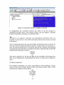
Design, Construction, and Testi ng of an
Electrodynamic Uniaxial Bench-Scale
Shake Table
Bill Wu
Advisors: Professor Erik Cheever and Professor Faruq Siddiqui
Department of Engineering
Swarthmore College
May 8th, 2015
1
Abstract
A bench-scale shake table was designed and constructed for the Swarthmore College
Engineering Department. The frame of the shake table was made of Unistrut. It's
powered by a motor with a complete built-in servo control system that takes analog
output as the velocity through an AID converter. Two transfer functions were
developed: one that connects the motor to the base plate and the other connecting
the plate to a simple test structure (lumped mass model). Sensors (LVDT and
accelerometers) were hooked onto the base plate and structure to measure
acceleration and displacement data to be sent back to Matlab for further analysis
and plotting. We used Matlab's linear simulator (lsim) to calculate the theoretical
output for a known input waveform, and compared the results to the actual
measured output (by the accelerometer). The results matched well for impulse
functions, step functions, and arbitrary waveforms such as the El Centro earthquake.
Two multi-story stick mass systems were shaken at their respective resonant
frequencies 0 bserve the effects of resonance.
2
Acknowledgements
I would like to thank Professor Cheever for his patience and wisdom along every
single step of this project. I also want to thank Professor Siddiqui for his guidance on
implementing testing structures, Professor Everbach for helping me understand the
previous codes developed for the motor at the start of the semester, Grant Smith
and James Johnson for their patience, guidance, and support in the machine shop, a
place I now no longer dread.
3
Table of Contents
Abstract
Acknowledgement
Table of Contents
1. Introduction
1.10bjective and Motivation
1.2 Key Components of the Shake Table
2. Construction
3. Theory
3.1 Derivation: Transfer function of a Second Order Underdamped System in
time and Laplace domain
3.2 Theoretical calculation: finding the resonant frequency of a lumped mass
system
3.3 Procedures for frequency domain analysis
3.4 Theoretical calculation: finding the resonant frequencies of a two-story
stick mass building
4. Animatics SmartMotor
4.1 Communication
4.2 Programming Notes
4.3 Motion Commands
4.4 I/O Ports
4.5 Analog Velocity
5. Data Acquisition (DAQ)
6. Calibration
7. Testing Structures
7.1 Lumped Mass System
7.2 Two-story Stick Mass Model
8. Results
8.1 The Big Picture
8.2 Comparing command input with measure velocity output
8.3 Obtaining Hplate
8.4 Obtaining Hstructure
8.5 Discussion on the significance of Hplate
8. 6 Using Matlab's LSIM
8. 7 Addition of a dash pot to enhance the El Centro simulation results
8.8 FFT analysis of two multistoried stick mass structure
9. References
Appendices
Appendix A: Matlab script file-Analog Velocity
Appendix B: Matlab script file-FFT Procedure
4
List of Figures
Figure 1: Animatics SmartMotor SM23165DT
Figure 2: National Instrument PCI-6221
Figure 3: AID Convertor Box
Figure 4: Linear Variable Differential Transformer (LVDT)
Figure 5: PCB 352B70 Accelerometer
Figure 6: Unistrut'" design and dimension of the shake table
Figure 7: LVDT stand
Figure 8: Dashpotstand
Figure 9: Mounting the SmartMotor onto Unistrut'"
Figure 10: Panoramic view of the shake table upon completion
Figure 11: Idealized Single DOF lumped mass structure used for testing
Figure 12: FFTofEI Centro acceleration response
Figure 13: Multimass-spring model for a two-story shear building
Figure 14: Frequency domain response to an impulse of a 2 -story structure
Figure 15: RS-232 Through USB for D-Style Motors MOOG Animatics (2014).
SmartMotor User's Guide
Figure 16: SmartMotor Interface example screenshot
Figure 17: Linear and sinusoidal motion
Figure 18: SmartMotor Connector Pinouts
Figure 19: Setup of the DAQ system
Figure 20: Test Run for calibration
Figure 21: Lumped mass structure used for testing
Figure 22: Two-story Stick Mass System
Figure 23: Connections details of the two-story stick mass system
Figure 24: The Big Picture
Figure 25: Command input and recorded input for an impulse
Figure 26: Command input and recorded input for a sinusoid
Figure 27: Command input and recorded input for the El Centro
Figure 28: Zoom-in of Figure 27
Figure 29: cftool to obtain curve fit for Hplate
Figure 30: Response to Impulse
Figure 31: Curve fit for Hstructure
Figure 32: Content of El Centro captured by Hplate
Figure 33: Theoretical and measured output for an impulse
Figure 34: Theoretical and measured output for a sinusoid
Figure 35: Theoretical and measured output for El Centro
Figure 36: Response to an impulse for more heavily damped system
Figure 37: Theoretical and measured output for El Centro for heavily damped
system
Figure 38: Time and frequency domain responses to an impulse of a 2 -story
structure
Figure 39: Time and frequency domain responses to an impulse of a 3 -story
structure
5
1. Introduction
1.1 Objectives and motivation
A bench-scale shake table can be a meaningful to study a model's response to a
variety of dynamic loading, including earthquakes, which are arbitrary waveforms.
The study of earthquakes is important because earthquakes cause billions of dollars
in damage every year around the world and tens of thousands of deaths and
injuries. In the United States alone, around 1,200 deaths have been recorded since
1900. Many more fatalities occurred in earthquakes elsewhere.
Buildings are normally adequately designed for gravity and vertical loads. Thus,
lateral movements provided by the uniaxial shake table can introduce bending to
the columns, and torsion if the center of mass and center of resistance are offset.
Testing of models of actual buildings and building prototypes is one method that is
useful in understanding the forces at work. Models built of plywood and aluminum
all-thread allow us to see the seismic behavior of a structure, and to understand how
the period of an earthquake if it is resonant with a building period, will cause the
most damage or even collapse.
The shake table is a device that simulates a dynamic loading or a seismic event. It
can also be used to create fictional "worst case" scenarios or resonant frequencies.
In computer controlled shake tables a computer program generates a signal, and a
digital signal is sent to a digitaljanalog converter, which sends a voltage to the
amplifier. The amplifier amplifies the voltage and sends it to the shaker platform to
which the model is attached. The constructed shake table is a one-degree of motion
shake table, meaning that it will move only in one lateral direction. A model on a
shake table with the same stiffness or resonant frequency as the prototype building,
will act in a way similar to that of the actual building.
1.2 Key components of the shake table
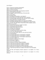
Motor: Animatics SmartMotor SM23165DT
The SM23165DT motor with HLD60 Internal Rollers and a stroke length of 400 mm
was chosen. The carriage shown in Figure 1 moves through a belt driven system
classified as a harmonic linear drive.
6
POWER & DATACONNECTION-:;,...::;..._~
DIMENSIONS ARE IN INCHES
Figure 1: Animatics SmartMotor SM23165DT
Data Acquisition (DAQ) system:
For our DAQ, we used a National Instrument PCI-6221, shown below:
Figures 2 and 3: NI PCI-6221 and its placement inside an AID convertor
We like it for its Correlated DIO, which enables digital and analog functions to be
synchronized with hardware-timed precision and reduced the need to write an
internal timer inside Matlab.
LVDT -Linear Variable Differential Transformer
The following figure depicts our LVDT:
7
Linear variable differential transformer (LVDT) is a type of electrical transformer
used for measurin g linear displacement. LVDis ar e inherently frictionless, and
converts a position or linear displacement from a mechanical reference into a
projXlrtional el ectrical signal containing phase and amplitude through induction
current . The calibration rat io is 1V = 10mm.
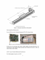
Accelerometer
The following figure depicts out accelerometer:
Figure 5: PCE 352E70 Accelerometer
8
The accelerometer is a device that measures proper acceleration ("g-force"). The
calibration ratio for our specific model is 1 V = 98.~m.
s
9
2. Construction
Construction of the shake table consisted of several key components, and a few
pieces of add-ons to support future additions to the shake table. The main frame
was first erected using Unistrue" pieces. Then, four pieces of cable hung from the
top frame pieces to support the base plate, which is a piece of plyvvood. The base
plate is then connected to the motor. Holders for the LVDT and dashpot were later
constructed and stabilized onto Unistrue" pieces.
A Unistrue" metal framing system was deemed optimal for the shake table's frame
as it can be used to support a large load while also be taken apart easily for storage.
The Unistrue" system contains specially configured '1ipped channels" made of
carbon steel that can be connected in a variety of configurations using fabricated
Unistrue" fittings.
Solidworks, a3D CAD modeling sofuvare was used to design the flume. The various
Unistrue" channels and fittings were obtained online from the Unistrue" CAD
Library. Different configurations of the channels were then considered to be built
around the dimensions of the flume. The final design of the frame is shown in Figure
ITEM NO
,,
,
,
0
,,,
,,
on
>0
DESCRIPTION
Uoidrv\, PIC«l
Uodrvl PI C«l
U 0 idrv t, PI C«l
Fittio9' (L-soap e" w i"91
LEN GTH
35 .20 io
';6 .37 io
';9.63 io
U 0 idrv l PI C«l
U 0 idrv l PI C«l
2';.00 io
17.21
"
,
,~~
Figure 6: Unistrue" design and dimension of the shake table
The holder for the LVDT is made of a hollow section aluminum bar, as shovm in
Figure 7:
10
Figure 7: LVDT stand
The easiness to make additions on Unistrut'" is manifested. The rod of the LVDT is
fastened to the base plate through a tapped hole. Also note that once the rod of the
LVDT is fastened to the base plate, there is a physical limitation to displacement of
the base plate. This won't cause too much inconvenience since our position
waveforms (integrated from velocity) is near symmetrical about zero so
displacement of the base plate is negligible.
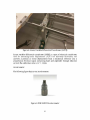
The holder for the dashpotis shown below:
Figure 8: Dashpot stand
The setscrews on the SmartMotor were carefully removed and preserved as we
detached the motor from the wave flume. The SmartMotor was mounted onto the
frame through two vertical aluminum beams, as shown in Fig. :
11
Figure 9: Mounting the SmartMotor onto Unistrut'"
The frame, cables, SmartMotor, base plate, and LVDT stand were completed within
the first three to four weeks of the semester. The need for a dashpot holder came
around the 12th week, by which time it was built by T' and attached onto the
structure. Upon completion, the complete view of the shake table is shown in Figure
10:
Figure 10: Panoramic view of the shake table upon completion
12
3. Theory
3.1 Derivation: Transfer function of a Second Order Underdamped System in time
and Laplace domain
Consider a mass-spring-damper system, with an input ofx(t). Equation of motion
will establish the following:
d 2y
dy
m+
c-+
ky = x(t).
dt 2
dt
Define the damping variable to be c:
Also recall that the relationship for resonant frequency is Wo
=
J¥;. Substituting the
above two equations into the equation of motion:
2
d y
dt
-2
dy
dt
2
+ 2(wo -+ woy =
2
Kwo x(t).
Performing Laplace transform on both sides of the equation we get:
Y(S)[S2
+ 2(wos + wJl
= KwJX(s)
Rearrange to get:
H(s) = Xes) =
Yes)
KwJ
S2
+ 2(wos + wJ'
which is the transfer function for a second -order underdamped system when the
input and output are both in terms of velocity.
Similarly, the transfer function for velocity in, acceleration out can be derived:
To obtain these transfer functions in the time domain, we can setup all the variables
using Matlab's symbolic toolbox and perform inverse Laplace through Matlab's
'iLaplace' command.
The time domain transfer function for velocity in velocity out is:
13
H(t)=l-
The time domain transfer function for velocity in acceleration out is:
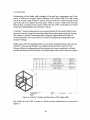
3.2 Theoretical calculation: finding the resonant frequency of a lumped mass system
The lumped mass system used and the cross section of the cantilever beam is shown
in Figure:
m
•
Y'
~~,} f .125"
10;
)
J
1"
Figure 11: Idealized Single DOF lumped mass structure used for testing
The second moment of area is:
,~
,
-bh'
,
~--in".
U
6144
The elastic modulus of aluminum is E = 10(10·)ps~ the weight of the aluminum
block (with the attached SparkRln accelerometer and ArduinoJ is W = 1.905 lbs,
the length of the cantilever beam is L = 26 u. Thus, we find the spring constant ofthe
lumped mass system:
k
~
3EI
lbs
= .278-.-.
L'
In
We can then find the resonant frequency wo:
OJ,
=
ffi
= 1 .19 Hz.
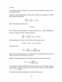
3.3 Procedures for frequency domain analysis
(Sample code for this procedure is attach ed in Append« B)
fft ~ h i ft Iff t Ib M~ Acc ~ ll;
dt= ti"", 12 1 -tim ~ III ;
Iti"'" I 1- Ib a~~ Acc ~ /21 I /dt/b M~Acc ~
FFT =
f= I 11 : l ~ ngth
;
p l otlf, ab ~ IFFTII
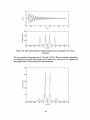
Performing this analys is on the £1 Centro acceleration response, we obtain the
folloVl'ing frequency -amplirude corr espondence:
Figure 12: FFT of £1 Centro acceleration respons e
3.4 Theoretical calculation: finding the r esonant frequencies of a """,-story stick
mass building
Th. tuilding to be ~yz.d i, th. ,~l. ,te.l rigid f~ shown in Fig .. The
weight' of u" floor '~ . u"
and ",,~=.d o ~ b.for. ass.mbl.d. It i, l1.,th ...
~ 'mll.d tho.tth. <lrucl\r.J propertt.,~. unifonn .Jongth. length of u" tuildin~
=.
W. rno doel the buildng ~, ~ two- .tory ,a,;r building, which => be "'Jres.d .d by
the spring-=" sy.t.m showninFig.
~t)
~-
"
f+.
,
i (r)
Figur. 13, M ulil='S-SJr~ mo doel for ~ two-<Iory
Th.
w. i ~
sh.~
bw ding
i, w.igh.din ltrn,
W,=W, = lIb
m, =m, =. OO 261b,'/in
Since the girdoer' or. =u:n.d 10 b. rigid, the <liffn." (,]ring
<Io ryi' giyenby,
•"= 12[(41)
,-
(»n~)
of ",ch
16.3 '"!
w in,
and u" indiYi<hU volues forth • .Jl-thr.~d'in <1 c ~ted
"
~. thu~
k, = k, = k = 1" 3~
ill
Th. ' 'J.'''lions of molionforth. sy'tem~. obbinod,
my', + k,y, - k, (y, -y,) = 0,
my', + k,(y, - y ,) = 0.
In u" usu;U =m ..., th. ", .qw.lions of lIDlion or. soly.d for h. Yib",lion by
,."b.tilU:ing,
y , = 0, 'in(""-~)
y, = 0, ' in(""- a)
y, = -o,""'in(""- a)
y', = -0,"" 'in(""-~)
Th •• xp=<ion of the d.temIil=l1 of the =trix fo",",lion of u" eqw.lions of
rnotton giyes a qw.<1'~ttc 'qu>lionin "" , =.ly,
ni",' - 3mk",' + k' = 0.
Sub.tilulion of u" mlll.ric volue , ju.t 0bt.in.d,
m'",' - 3mk",' + k' = 0.
Th.r.for~ the ""tur.lfr.quencies ofth. <lructur.~"
W1 = 8.69HZ;
w,
= 20.59 Hz.
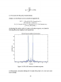
Recall the FFT analysis of the data obtained via an impulse on the two-story
building:
_ __ __ _- _ ,
'm
~~~-
Cm'---,~c---.~
~--.~~'-'o"c"-'"c'--',~c~'~~--"~'--',~c--~m
°r.q (Hz)
Figure 14: Frequency domain response trJ an impulse of a 2 story structure
The actual natural frequencies are:
w1 = 6.1Hz; w, = 19.2Hz
17
4. Animatics SmartMotor
4.1 Communication
The Animatics SmartMotor is electrically driven which enables the creation of
arbitrary waveforms as opposed to only hardcoding waveforms using discrete data
points of velocity, position, etc. The motor communicates through a PC serial port
via a RS232 port A single connection to the 7 -Pin Combo D-Sub Power & I/O
provides power and communication to the motor using a CBLSM1-xM cable. The
motor can be powered using a 24-48 VDC power supply. An Agilent N5746A power
supply was used which has a DC output voltage rating of 40 V. 19 A current and 760
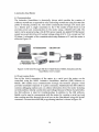
W power. A schematic of the communication setup betvveen a PC and the motor is
shown in Figure 15:
KITUSB232485
CBLSM1-xM
PS24V8AG-ll0
or PS42V6AG-l10- "J;:::'-- Figure 15: RS-232 Through USB for D-Style Motors MOOG Animatics (2014).
SmartMotor User's Guide
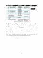
4.2 Programming Notes
Due to the direct connection of the motor to a serial port, the motor can be
controlled using the MOOG Animatics SmartMotor interface (SMI) Software or
Matlab. SMI enables easy communication through the terminal program which
provides immediate response to a given command. Additionally the SMI softvvare
contains debugging options and can obtain information from the motor including
current position, velocity, acceleration and voltage. Because of these characteristics,
the SMI software is ideal for troubleshooting. In addition to the SMI software.
Matlab can be used to communicate with the motor by creating a serial port and
then sending text files through the serial port to the SmartMotor using the 'fprintf
command. Ascreenshot of the SMI programming interface is shown in Figure 16:
18
Tem,inal
FnJ Mot",s
s-
De te cte d Config..-ation
raJ} Com3 (AS232-96W bps)
~ Motor1-C0m3 (50 0 )
C
!
"~~
C,"
CAN
C~
0 (1 2500) bps)
Figure 16: SmartMotor Interf;;Ce
exaffipIe sc;re<mshot
In configuration, the mnnection betvveen the motor to the PC com-port is
established through 'Com3'. The terminal window acts like Matlab's command
window. Commands can be given to control the motor.
WI allows
us to upload a script file onto SmartMotor's hard-drive. Only one
program can be stored at a time. With each upload, the previous version is erased
and replaced.
Prior to llKlving the motor, the over-travel limits and fault bits must be cleared. To
clear the over-travel limits, the EIGNQ command, "Enable Inputs as General Use", is
used. The historical fault bits are cleared by using the ZS mmmand. The following
command lines must therefore be included in all code or typed directly into the SMI
terminal before the motor can move.
EIGN(2)
EIGN(3)
ZS
After these mmmands are set, the LED light on the SmartMotor will change from
solid red to flashing green indicating that the motor is ready and on standby to
move.
4.3 Motion Commands
The Animatics SmartMotor can move using different modes including a torque
mode, velocity mode, absolute position mode, and relative position mode. A basic
absolute move example is shown below:
MP
VT=100000
ADT=1000
PT=20000
G
19
The velocity, acceleration, and position are given in encoder units. A conversion is
therefore necessary to specify the position in inches, velocity in inches per second,
and acceleration in inches per second squared. The Animatics SM2316SDT used in
this project rotates with 4000 encoder counts per revolution. Additionally the
HLD60 Actuator with Internal Rollers has a 12.5 mm displacement per revolution.
Using simple programs, we can achieve linear and sinusoidal motion, as depicted by
Figure 17:
Test Run; Linear Moti on (2.1em/a)
Te st Ru n· Sinus oida l Moti on
"
"
H
~>32
i
"~-...............,.....,,...-~
~28
n
'c,~7-~-7~--~;~~~7-~,~w
°O~~O~
5 --~~,7
5 --~
' ~'~
.5 --7--3~5~
,~.
time
Figure 17: Linear and sinusoidal motion
However, SMI programs are only good for achieving relatively simple motion. A
comprehensive list of desired position and/or velocity needs to be hardcoded into
the program. This is not practical when we're ultimately trying to implement an
arbitrary waveform. For example, if the waveform of velocity data is spaced at 20ms
and has a duration of 30s, there are 1,500 velocity data points to write into the SMI
program, which is not realistic or desirable.
4.4 I/O Ports
Upon further study of the User Manual, we discovered the SmartMotor's I/O
Functions, which are extremely flexible and provide a variety of digital and analog
input and output capability. Each I/O point has a corresponding pre-assigned
variable name within the programming environment and can be read from, or
written to, by placing it on the right or left side of an equation, respectively. The
SmartMotor SM2316SDT is equipped with 15 I/O points, which can be physically
accessed by a DB-iS D-sub Connector. The pin numbers and their corresponding
functions are listed in the following:
20
PIN
,
,
,
,
,
,
,•
"'"
""
"
.
5V 1/0 Connector
--------10Bit 0-5VDCMl
_....
10Bit O-5VDCMl
1.!iMI-Iz max as Ene. Or
Dr. q,ut
S eClflcatlons
I/O - 0 GP or Ene.Aor step q,ut
I/O - 1 GP or Ene. B or Dr_q,ut
1/0 - 2 Posi!iveOIt!fTravei orGP
Notes
1.!iMI-Iz max as Ene or
Ola ram
00-15 O... ub Connector
10Bit 0-5VDCMl
I/O - 3 Neo;Ja1iYe OYer TfOI'Iel or GP
10Bit O-5VDCMl
00 - '
GPor RS485ACorn(II
1152KBaud M:llI
10Bit O-5VDCMl
I/O - 5 GP or RS--485 B Corn(I)
1Ul111
I/O -
fj
"G' COIIlINr'd or GP
115.2KBoud M:llI
U-~VUGMJ
IIlB1t 0-5VDCMl
Phase A Enaxler 00..CjlU
Pm ... B Encode< 0Uput
RS-232 Tf3I5M Corn(O)
RS-232 Rece<ve Com(ll)
.~~
1152KBaud Mal!
115.2KBaud M:llI
~
~
Main f'ufIoc *12.!VllC
to *4l!VDC
If -DE 0pIi0n, Conlrol _
""""",Ie !TOm ~ _
WillI -DE option, I!lis
be<:omes seP:IJ:lte
cortmIJXM'<!fF4U.
Figure 18: SmartMotor Connector Pinouts
The 5V I/O is push-pull. To use the I/O functions, in our code we must first
deactivate default on-board I/O functions. To take inputs, the following command is
useful:
INAeVl, exp),
where "exp" is the I/O Bit Number or Status Word Number. This can be passed in
from a variable.
4.5 Analog Velocity
From the User Manual, we found the following sample code, based upon which we
were able to achieve motion based on an analog outputofvelocity:
21
l':IGN ( W, O}
'Di ~,. bl e
J<;P= 3020
= = 100 1 0
fxom d e faul t
'Incx ea ~e damping f rom d e f a ul t
'Ac t ivate new tuning pa r a me t e r~
'Se t max imum acc~lerAtion
'Se t t o Mod~ Ve locity
'Anal o g d e ~d band, 5 000 = full ~ cale
'Of f ~ et to Allow n e g a tive ~ "~ng ~
'Mul t ipli~r f or ~ pe ed
'Time d e l a y b e twee n r e,. d ~
'See d b
'L a b"l t o create infini t e loop
'Tak~ anAlog 5Vol t l"S reading
'S e t x t o det e rmine ch a nge in inpu t
'Ch ~ ck if chang e b e yond d ea dband
'Mult1p11 e r tor .ppropr1ate ~ pe e o
'Ini t iate new v e locity
'Ch e ck if chang e beyond d ea dband
'Multipli~r f or appropriate ~ pe e d
'Ini t iate n e w velocity
'End I f ~ t ~ t ement
'Updat e b f o r pr e v e ntion o f hunting
'P " u ~ e b e for e n e xt r e ad
'Loop b a ck t o l abe l
'Obligatory END (neve r r e ached)
,
ADT= 100
~
d = 10
0 =2500
m= 4 0
.,= 10
b =O
c>o
a = INA (V1 , 3} - 0
x=a - b
II" x >d
VT =b ' m
C
ELlll:Il" x < - d
VT= b ' m
C
l':NDU'
b =,.
WAIT= w
GOTOl O
,=
'Incx e a ~e
h~xd" ,. x e
limi t ~
~ t iffn e~~
A deadband is an interval of a signal domain or band where no actbn occurs (the
system is dead). For our purpose, however, the input are waveforms that could be
considered digital (signal is constantly changing) and thus setting the deadband to
10 is detrimental to obtaining consistency. We changed d to O.
To achieve a maximum speed of aroundO.1 mis, we experimented with the
multiplier value and changed it from40to9 5. The wait time is decreased to 5
(w = 5) to acoomrmdate higher sampling r ates.
The rmstirnportant line of this sample code isthe following:
a=INV(V1,3)-0
INV(V1,3) means vve are retrieving input from I/O point 3, or pin number 4. Voltage
is also scaled in millivolts where 3456 VIOuld be 3.456V. Setting the offset to 2500
(0 = 2500) means the 2.5V is the zero-velocity voltage.
This code causes the SmartMotor's velo ely totrack an an a log input.
22
5. Data Acquisition System
Data acquisition plays an important role in connecting Matlab and the SmartMotor.
It queues the desired waveform sent from Matlab in an array format. While the
SmartMotor is activated, its code retrieves the line of data to use as the velocity
19:
The basic
Figure 19: Setup of the DAQ system
As shown in Fig., the analog output portion of the A/D converter is then connected
to Pin 4 and 'ground' of the SmartMotor's I/O port. On the analog input section of
the convertor, two connections go the accelerometer and LVDT's power source,
respectively.
It is largely realized through Matlab's data acquisition toolbox. With the toolbox we
can configure data acquisition hardware and read data into MATLAB and
Simulink for immediate analysis. We can also send out data over analog and digital
output channels provided by data acquisition hardware.
In Matlab, we create a session object that we can configure to perform operations
using a CompactDAQ device:
w = daq.createSesion('ni'),
where 'ni' is the name of the vendor.
To collect data from our LVDT and accelerometer, we added two analog input
channels to Matlab's DAQ session. To store data, we created one analog output
23
channel. After the desired waveform is generated inside a vertical array, we transfer
it into the DAQ through the following command in Matlab:
queueOutputData(w, motion)
To collect the data that the sensors collect during motion, we used the following
command:
data = w. startForeground( );
'Data' will consist of two columns: acceleration and displacement, both in terms of
voltage. Using the calibration ratios given in the Introduction section, we can obtain
the acceleration and speed in terms ofSI units:
a = data(: ,1) * 98.1 ...... (m/5 2)
x = data(: ,2) * .01 ...... (m)
24
6, Calibration
While we transfer data from Matlab to the SmartMotor thrcugh the DAQ system, the
array is seen as voltages, not velocity in SI units. Calibration is nealed so we can
input waveforms of velocity in terms of SI units (m/s),
We tOClk a sample test run, Fig, , depicts time and JX'sition voltage on the two axes,
By calculating the slope through extracting two data points, we found the actual
velocity to be 2, 1 em/s, The voltage fed into the DAQ was 3,04V, Taking into account
the 2,5V offset in our analog velocity code, we calculated the conversion ratio from
SI units to SmartMotor voltages:
calibration ratio
,021m
=
(3,045
2,5)V
,0385
Test Run: Linear Motion (2.1 emfs)
"
W
•rn e
•
">
0
0
~
"
"
0
0
0
,
o
ccc'---'oc;c----c---"c;c---"c---"O;c---CC---;,";----~,
time
Figure 20: Test Run for calibration
Thus, in our Matlab code, we added the following line for unit conversion:
motion
=
2,5
[v I
+ -""",.
, 0385'
where [v 1is the vertical array of analog velocity of the waveform to be queued into
the DAQsystem,
25
7. Testing Structures
7.1 Lumped Mass System:
The lumped mass system used is shown in Figure 21:
Figure 21: Lumped mass structure used for testing
The second moment of area is I
= 2..bh 3 =
12
_1_
6144
in4. The elastic modulus of
aluminum is E = 10(10 6 )psi, the weight of the aluminum block (with the attached
SparkFun accelerometer and Arduino) is W = 1.905 Ibs, the length of the cantilever
beam is L = 26". The spring constant of the lumped mass system is k = 3~1 =
Ibs
.
.278 -.
. The resonant frequency IS
wa
In
=
Ng
- =
W
7.2 Two-story Stick Mass Model
The model is shown in Figure 22:
26
t
1.19 Hz.
Figure 22: Two-story Stick Mass System
The columns are aluminum all-threads with a diameter of 0.186". The two stories
are made from 1/8" plywood, and weigh 1 lb. They are equally spaced along the
column, with each story 8" in height. At the support, the aluminum square plate had
%" tapped holes, which was bigger than the diameter of the selected all-thread. A
special nut was made on the lathe to fit both the tapped hole on the aluminum
square plate as well as the all-thread. 10-32 nuts were used to stabilize the two
stories so they wouldn't move along the column, even during high frequency motion.
Details of the special nut and the 10-32's are shown in Figure 23:
Figure 23: Connections details of the two -story stick mass system
As shown in the Theory section, the resonant frequencies are Wi = 8.69Hz; w 2 =
20.59 Hz. The three-story stick mass system is identical in nature, and therefore is
not shown in this report.
27
8. Result
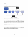
8.1 The Big Picture
The system outline of the shake is shovm below in Figure 24:
Construction
t
.. .. -
/
\.
Base
Plate
I
Figure 24: The Big Picture
8.2 Comparing command input vvith measure velocity output
Mter we calibrated the SmartMotor's analog velocity program, we experimented
vvith a variety of input. We queued an impulse, sinusoid, and the El Centro into the
A/D converter and recorded the base plate's position using the LVDT. We then
plotted both the differentiated LVDT data (to 0 btain velocity) with the input velocity
against time.
Comparing command input w ith measured velocity
For an impulse, the Matlab command is:
o n e~
(1 0 , 1 ) * 0 . 0 9 2 ;
Since the sample rate of the created DAQ session is 100 Hz, our input impulse has a
duration of 10/100=0.ls at .092 m/s. At other times, the input velocity is zero. The
described vvaveform is depicted precisely by blue in Figure:
28
Imp ul se
"
0,08
,
0,06
c
,
0
••
••
0,04
002
0
-D,0 2
tim e
Figu re 25: Co mm and Input and rec orded Input for an Impul se
me
The more 1I018y gree n d.t:l Is the po sldo n data me.rured by
LVDT, obooined
from ou r DAQ' . se co nd analog InPUt chann el (m e nrst Input channel Is reserv ed fc>r
the I ccelerado n data, which Is mentio ned late r), Note mat the re Is an awroxim ately
70 ms delay at me bas e pl ate' . fir st i ign of accelerati on. At this point we can not
evaluate the signifbnce of this time l.g wk:hout qua ntifying the transfer functlon
ben.tee n th e maror an d th e base pl.Ql . We \1\11\\ noW r efer m that tr.n sfer fun cclo n as
H ... . ,
For a sinusoid, th e Matlab co mm and is :
..1 '
. 0 6Z · .in( 19. ·
ti ••
'I,
Like Vl'ith th e impul se, We plotted the inputw,vefc>rm al<mg with the differentlatlld
LVDT data to obOli n Figure:
Sinusoid
tim e
Figure 26: Command input and recorded input for a sinusoid
There is an apparent time lag. but
peak amplitude and period.
otherwi~
the two match peIfectly in terms of
For the El Centro, we obtained the El Centro north-oouth acceleration data, and then
performed Euler integration to get velocity (sample code attached in Appendix B).
The Matlab command to create the input waveform is:
We then pbtted the input waveform along with the differentiated LVDT data to
obtain Figure:
30
5
""5
E
•••
~
1.5
0.5
2
3
li me
2.5
3.5
4
4.5
5
5.5
Figure 27: Command input and recorded input for the El Centro
8.3 Obtaining
Hplate
To gain a close look, we zoom in on the first 100 ms of the impulse inputjLVDT
result (Figure):
,
I
gO. C6
.1"
,
,
1l 00
c
All
\A All
A
"
time
Figure 28: Zoom-in of Figure 27
31
A
Create arrays for the time and base plate position and use Matlab's curve fitting
toolbox:
0.1
O.[)l
"
~O CE
""
"
•
0.04
base~ V$ , ~m ~
- - Plate TrlllSfer FLn::!Xfl
002
0
0,02
0,04
0.00
timehp
O.[)l
0.1
0,12
Figure 29 : cftool to obtain curve fit for Hp1ate
The curve fitting results are as follov.rs:
1
Wo
= 52.7; \ = 0.60; T = - , = 0.03 (R 2 = 0.8 1)
we>
Note that Hplate's time constant T is only 0.03 seco nds, which also translates to a
cutoff frequency of around 5 Hz.
8.4 Obtaining Hst'nlcture
To obtain the transfer function of th e lumped m ass structure, we applied the same
impulse and obtained the fo llovving acceleration output results:
32
.,,-------------------,
, '-'---~c_-~c_-~o_-~ec_----c'.
o
5
10
15
W
~
tim e
FigW'e 30: Response to Impulse
Create array s for the time and structure acceleration and use Matlab's clI"Ve fitting
toolbo x:
••
•
~
• t •
baseAhs vs. omens
- - Struct1.re Tr¥1Sfer Ft.n::tion
•
•
It.
0.5
•
1
~
0
~.5
•
o
•
, •
6
•
• •
• •
•
,
" "
l lmehs
" "
Figure 31: Curve fit for Hstructure
The curve fitting results are as folloVIIS:
Wo
= 6.6; ( = 0.003 6;'£ =
1 7 = 42 s (R 2 = 0.8 7 ).
w"
Notice the time constant is much bigger than that of Hp1are . This give us a valid
reason to ignore H p1aI e .
33
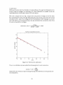
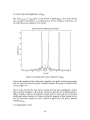
8.5 Discuss ion on the significance of H .....
The fact,,,,,,,,,,,,.» 'vbto give, us one reason to ignoreHvbto ' Al,o recall that it,
time constant correspond, to a cutoff frequency of 5 Hz. Plotting a vertical line of 5
Hz onthe frequency-amplirude orEl Centro:
EI C.... ro fre qu erry />m pll: ud. C"''' pond"",.
,
,
freq(Hz)
Figure 32: Content of £1 Centro caprured by Hv>Db,e tve the majority of the earthquake" amplirude are in the low frequency region,
a nd are caprured by the ba se plate" transfer IJnction. This points to another valid
reason to ignore it
Based on the fact that the base plate" transfer IJnctioo has a significantly smaller
time constant compared to that of the 'tructlJre'" and that it, cutoff frequency is
higher enough to capture the majority content of the £1 Centro (in fact most major
earThquake ..,have simlar to £1 Centro, in that the majority of their content lie, in
the low frequency region), we have decided to ignore the base plate" transfer
functlon,H......
8. 6 Using Madab', L51 M
ls im simulates the (time) response of continuous or discrete linear systems to
arbitrary inputs.
ls im (sys, u, t) produces a plot of the time response of the dynamic system
model sys to the input history, t, u. The vector t specifies the time samples for the,
and consists of regularly spaced time samples. The input u is an array having as
many ro'WS as time samples and as many colunms as system inputs. For instance,
if sys is a SISO system, then u is a t-by-l vector. If sys has three inputs, then u IS
a t-by-3 array. The model sys can be continuous or discrete, SISO or MIMo.
Since our system is a discrete SISO, both u and t have only one column. After
obtaining the structure's transfer function, Hstructnre, we obtained the theoretical
acceleration output for three types of command input (impulse, sinusoid, and El
Centro) to see how well they compare.
For the Impulse input, the 1 sim result is in blue, while the measured acceleration
by the accelerometer is in green:
Impulse
oe
06
"'
"0
~,
~,
~6
·1
0
2
3
,
5
6
7
Figure 33: Theoretical and measured output for an impulse
For the Sinusoidal input, the 1 sim result is in blue, while the measured acceleration
by the accelerometer is in green:
35
Sinusoid
2
1.5
1
0. 5-~
o
-0 .5
·1
·1 .5
·2
05
1
1.5
2
2.5
3
35
4
4.5
5
5.5
Figure 34: Theoretical and measured output for a sinusoid
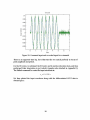
For the El Centro, the lsim result is in blue, while the measured acceleration by the
accelerometer is in green:
EI Centro
-0.8
Figure 35: Theoretical and measured output for El Centro
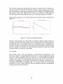
We see that the lsim results for impulse and sinusoid input are good in in terms of
amplitude and frequency. They are both for relatively short durations. For the El
Centro output, we can see the basic shape of the predicted result matches that of the
measured acceleration. However, there is a noticeable shift throughout the entire
waveform starting before the first second.
8.7 Addition ofa dashpotto enhance the El Centro simulation results
We then speculated the cause of the shift for the lsim results for the El Centro.
Recall that our structure system is very lightly damped, with a damping coefficient
of near zero (( = .0036) and the time constant of over 30 seconds. Such light
damping could cause the delay in response, which is then amplified by the long
duration of the El Centro waveform.
36
To verify our speculation, we added a dashJXlt stand onto our frame (again, made
easy by choice of our framing material-Unistrut™). The rod of the dashJXlt is
fastened onto the structure by gluing a No.5 nut onto its front surface. There is a
even great limit to the amount of possible displacement as the dashpot's rod is even
shorter than that of the LVDT. Due to this limitation, we could only run a five second
waveform of the El Centro.
First, we found the transfer function for our more heavily damped system by
applying an impulse and measuring the acceleration response using the
accelerometer:
"
time
Figure 36: Response to an impulse for more heavily damped system
We then imported this data into Matlab's curve fitting toolbox and found the
following results:
1
Wo = 7.267;t; = 0.08;T = - = 1.7 (R2 = 0.38)
W o\
Note the increased damping coefficient and the significantly smaller time constant.
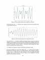
We then coded this transfer function into Matlab's workspace and performed lsim
on just five seconds ofEi Centro:
37
Figure 37: Theoretical and measured output for El Centro for heavily damped
system
Note that shiftin g only started after the third second mark, which shows an
improvement from the previous system.
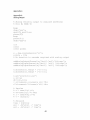
8.8 FFT analysis of two multistoried stick mass structure
We constructed a twos-story stick mass model, as shown in the Theory section. Each
floor was sawed from 1/2/' plywood at the woodshop, then drilled with a No. 12
drill at the four corners, which are spaced to match the four aluminum square plates
on the four corners of the shake table. 32-thread/inch aluminum all-threads with a
.186" diameter was used as the columns. Connection details are also shown in the
Theory section.
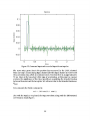
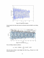
To find the structure's resonant frequencies, we shook it using an impulse. Our PCE
accelerometer was fixed onto a nut glued on the top floor. The aCCEleration response
was plotted, and then we applied the FFT procedure to obtain the frequency domain
information:
m
;
<•
•"
"
c
~
m
c
0;
,
,
;
Time
,
"
"
,
4.0
'ill
'''"
"
e•
~
"•
10J
c
·ffi
I,
" "
.",
m
""
0
Freq (HI)
m
'" " "
ffi
Figure 38: Time and frequency domain responses to an impulse ofa 2-story
structure
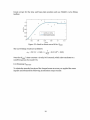
The two reoonant frequencies are 6.1 Hz and 19.2 Hz. This is a standard procedure
for finding the reoonant frequencies of the multi-story structures. We applied the
same approach to a three-story stick mass structure:
39
Figure 39: Time and frequency domain responses to an impulse of a 3 -story
structure
40
9. References
Engineering 12 Website, Erik Cheever
Structural Dynamics-Theory and Computation, Mario Paz
MOOG Animatics. (2014). SmartMotor User's Guide:
Technology. Moog Animatics.
Class 5 SmartMotor
Unistrut. (2013). Unistrut. Retrieved January 2014, from Atkore International, Inc.:
http://www.unistrut.us/
41
Appendices
Appendix A
Analog Output
% Analog velocity output to simulate waveforms
% Bill Wu ENGR 90
beep
disp( 'xxx');
specify_position;
pause(3);
beep
pause(O.l)
disp( 'yyy');
clf
clear
clear global
w ~ daq.createSession('ni');
w . Ra t e ~ 100;
% No duration in seconds required with analog output
addAnalogOutputChannel (w, 'Dev3 ' , 'aoO' , 'Vol tage' ) ;
addAnalogInputChannel(w,'Dev3', 'aiO', 'Voltage');
addAnalogInputChannel (w, 'Dev3', 'ail', 'Voltage');
w .Channels(l).Range
w.Channels(2).Range
[-10 10J
[-10 10J
load ( 'elcentrino. mat' )
a
el=-a;
dt~t(2)-t(1);
v
x
a el-mean( a el)) *dt;
el~cumsum(v el-mean(v ell )*dt;
el~cumsum(
% Impulse
% s ~ ones(10,1)*0;
% ss~ones(10,1)*0.092;
% r
ones(400,1)*0;
% v ~ [s;22;rJ
% Sinusoid
time ~ 0:dt:10;
ssl
.04*sin(1
ss2 ~ .04*sin(2
* time');
* time');
42
ss3
.04*sin(3 * time');
ss4
.04*sin(5 * time');
ss5
.04*sin(7
* time');
v = [s;ssl;ss2;ss3;ss4;ss5;rJ;
cf:
0.04*(1-1/sqrt(1-z A2)*exp(-z*w*x)*sin(w*sqrt(1A
z 2)*x) )
% cff:
c*w A2*exp(-x*w*z)* (cosh(x*w* (z A2
1)A(1/2))
( z * sinh (x * w* (z A2 - 1) A ( 1/2) ) ) / (z A2 - 1) A (1/2) )
%
% El Centro
% v
v el(l:lOOO);
~
Basemotion
~
2.47 + v/0.0385;
queueOutputData(w,Basemotion);
s ~ serial('COM3'); % creates serial port object for motor
% set all the properties of the port
s.BaudRate
9600;
s. DataBits
8;
s.Terminator
'LF/CR';
s.RequestToSend
'off' ;
s. FlowControl
'software' ;
s.DataTerminalReady
'off' ;
s.parity
'none' ;
fopen(s); % connect serial port object to the motor
disp( 'Connected to motor'
% remove hardware limits, set velocity and acceleration
initialize ~ ['EIGN(2) EIGN(3) ZS'];
fprintf(s, initialize)
go ~ [' RUN' ] ;
fprintf(s, go)
%Use the start Foreground function to start the
analog
output ...
%operation and block MAT LAB execution until all data is
generated.
data
~
w.startForeground();
% After excution of analog output, tell motor to rest
command
['MV VT~O ADT~200 G END'];
43
fprintf(s,
command)
fclose(s);
% close serial port cleanly
hold off
pause(l)
time ~ ((l:size(data,l))-l)/w.Rate;
baseA ~ data(:,1)*98.1;
baseP ~ data(:,2)*O.Ol;
baseV~diff(baseP) ./(diff(time' I);
baseV(end+l)~baseV(end) ;
%baseV ~ smooth(baseV);
plot(time,v,time,baseV),xlabel('time' ),ylabel('base
motion' )
%1 egend ( 'Comma nd ' , 'Output' ) ;
%subplot(2,1,1) ,
plot(time,v) ,xlabel( 'time') ,ylabel( 'Command')
%subplot(2,1,2) ,
plot(time,baseA),xlabel('time' ),ylabel('Output')
figure
plot(time, baseA)
% figure
%
plot (time,data (:,1) ), xlabel ( ' time' ) , ylabel (' accel
voltage')
beep
disp( 'zzz'
44
Appendix B
FFTcode
load two story
subplot 12, 1, 1);
plotltime,baseA);
xlabel I 'Time'); ylabel I 'baseA' );
subplot 12, 1, 2);
bFFT ~ fftshiftlfftlbaseA));
dt~time(2)-timel1) ;
f~ I 11: length Itime) ) - I length I baseA) /2) ) /dt/ length I I baseA) ;
plot I f, abs IbFFT) )
xlabell'Freq 1Hz)'); ylabell'abslfftlbaseA))');
45