1
VYSOKÉ UČENÍ TECHNICKÉ V BRNĚ
BRNO UNIVERSITY OF TECHNOLOGY
FAKULTA INFORMAČNÍCH TECHNOLOGIÍ
ÚSTAV INTELIGENTNÍCH SYSTÉMŮ
FACULTY OF INFORMATION TECHNOLOGY
DEPARTMENT OF INTELLIGENT SYSTEMS
RECOGNITION OF VEHICLE NUMBER PLATES
BAKALÁŘSKÁ PRÁCE
BACHELOR´S THESIS
AUTOR PRÁCE
AUTHOR
BRNO 2007
ONDREJ MARTINSKÝ
VYSOKÉ UČENÍ TECHNICKÉ V BRNĚ
BRNO UNIVERSITY OF TECHNOLOGY
FAKULTA INFORMAČNÍCH TECHNOLOGIÍ
ÚSTAV INTELIGENTNÍCH SYSTÉMŮ
FACULTY OF INFORMATION TECHNOLOGY
DEPARTMENT OF INTELLIGENT SYSTEMS
ROZPOZNÁVÁNÍ EVIDENČNÍCH ČÍSEL VOZIDEL
RECOGNITION OF VEHICLE NUMBER PLATES
BAKALÁŘSKÁ PRÁCE
BACHELOR´S THESIS
AUTOR PRÁCE
ONDREJ MARTINSKÝ
AUTHOR
VEDOUCÍ PRÁCE
SUPERVISOR
BRNO 2007
DOC. ING. FRANTIŠEK ZBOŘIL, CSC.
[Note for binding – place for a copy of the thesis submission]
iii
[Note for binding – place for a copy of the license, page 1]
iv
[Note for binding – place for a copy of the license, page 2]
v
Abstrakt
Práce se zabývá možnostmi využití teoretických poznatků z oblasti umělé inteligence,
strojového vidění a neuronových sítí pri konstrukci systémů pro automatické rozpoznávání
evidenčních čísel vozidel. Do této problematiky spadají matematické principy a algoritmy, které
zabezpečí detekci oblasti evidenčního čísla vozidla, segmentaci, normalizaci a samotné
rozpoznání znaků. Práce komparativním způsobem pojednává o možnostech zabezpečení
invariance systémů z pohledu světelných podmínek nebo deformace obrazu z pohledu kamery,
kterou je obraz snímán. Součástí práce je také implementace demonstracního modelu, který je
schopný tyto funkce realizovat nad sadou statických snímků.
Klíčová slova:
Strojové vidění, umělá inteligence, neurónové sítě, optické rozpoznávaní znaků, ANPR
Abstract
This work deals with problematic from field of artificial intelligence, machine vision and neural
networks in construction of an automatic number plate recognition system (ANPR). This
problematic includes mathematical principles and algorithms, which ensure a process of number
plate detection, processes of proper characters segmentation, normalization and recognition.
Work comparatively deals with methods achieving invariance of systems towards image skew,
translations and various light conditions during the capture. Work also contains an
implementation of a demonstration model, which is able to proceed these functions over a set of
snapshots.
Key Words:
Machine vision, artificial intelligence, neural networks, optical character recognition, ANPR
Bibliographical citation
Ondrej Martinský: Recognition of vehicle number plates, bakalářska práce, Brno, FIT VUT v
Brně, 2007
vi
Declaration
I declare that I wrote this thesis myself with the help of no more than the mentioned literature
and auxiliary means.
........................................
Ondrej Martinsky
Acknowledgement
The author is indebted to the supervisor of this thesis, doc. Ing. František Zbořil, CSc. for his
great help.
Copyright © 2007 Ondrej Martinsky
THIS WORK IS A PART OF THE RESEARCH PLAN "SECURITY-ORIENTED
RESEARCH IN INFORMATION TECHNOLOGY, MSM 0021630528" AT BRNO
UNIVERSITY OF TECHNOLOGY
Licensed under the terms of Creative Commons License, Attribution-NonCommercial-NoDerivs
2.5. You are free to copy, distribute and transmit this work under the following conditions. You
must attribute the work in the manner specified by the author or licensor (but not in any way
that suggests that they endorse you or your use of the work). You may not use this work for
commercial purposes. For further information, please read the full legal code at
http://creativecommons.org/licenses/by-nc-nd/2.5/legalcode
vii
Contents
1 Introduction
1.1
1.2
1.3
1.4
1
ANPR systems as a practical application of artificial intelligence
Mathematical aspects of number plate recognition systems
Physical aspects of number plate recognition systems
Notations and mathematical symbols
2 Principles of number plate area detection
2.1
2.2
2.3
2.4
2.5
Edge detection and rank filtering
2.1.1 Convolution matrices
Horizontal and vertical image projection
Double-phase statistical image analysis
2.3.1 Vertical detection - band clipping
2.3.2 Horizontal detection - plate clipping
Heuristic analysis and priority selection of number plate candidates
2.4.1 Priority selection and basic heuristic analysis of bands
2.4.2 Deeper analysis
Deskewing mechanism
2.5.1 Detection of skew
2.5.2 Correction of skew
3 Principles of plate segmentation
3.1
3.2
Segmentation of plate using a horizontal projection
Extraction of characters from horizontal segments
3.2.1 Piece extraction
3.2.2 Heuristic analysis of pieces
4 Feature extraction and normalization of characters
4.1
4.2
4.3
Normalization of brightness and contrast
4.1.1 Histogram normalization
4.1.2 Global thresholding
4.1.3 Adaptive thresholding
Normalization of dimensions and resampling
4.2.1 Nearest-neighbor downsampling
4.2.2 Weighted-average downsampling
Feature extraction
4.3.1 Pixel matrix
4.3.2 Detection of character edges
4.3.3 Skeletonization and structural analysis
5 Recognition of characters
5.1
5.2
1
1
2
3
5
5
5
7
8
9
10
13
13
14
15
16
18
20
20
22
22
23
25
25
25
27
28
29
29
30
31
31
32
35
42
General classification problem
Biological neuron and its mathematical models
viii
42
43
5.3
5.4
5.5
5.2.1 McCulloch-Pitts binary threshold neuron
5.2.2 Percepton
Feed-forward neural network
Adaptation mechanism of feed-forward neural network
5.4.1 Active phase
5.4.2 Partial derivatives and gradient of error function
5.4.3 Adaptation phase
Heuristic analysis of characters
6 Syntactical analysis of a recognized plate
6.1
Principle and algorithms
6.1.1 Recognized character and its cost
6.1.2 Syntactical patterns
6.1.3 Choosing the right pattern
7 Tests and final considerations
7.1
7.2
44
45
46
47
48
49
50
53
56
56
56
57
57
59
Choosing the representative set of snapshots
Evaluation of a plate number correctness
7.2.1 Binary score
7.2.2 Weighted score
Results
59
60
60
61
61
Summary
Appendix A: Case study
Appendix B: Demo recognition software – user’s manual
Bibliography
62
63
73
76
7.3
ix
List of Figures
1.1.a
1.1.b
2.1
2.2
2.3
2.4
2.5
2.6
2.7
2.8
2.9
2.10
2.11
2.12
2.13
3.1
3.2
3.3.a
3.3.b
4.1
4.2
4.3
4.4
4.5
4.6
4.7
4.8
4.9
4.10
4.11
4.12
4.13.ab
4.13.c
4.14
5.1
5.2
5.3.a
5.3.b
5.4.a
5.4.b
5.5
5.6
5.7
5.8
7.1
Illuminated number plate
Snapshot degraded by the significant motion blur
Convolution matrix
Various rank and edge detection filters
Vertical projection of an image into a y axis
Double-phase plate clipping
Vertical projection of the snapshot after convolution with a rank vector
Band detected by an analysis of a vertical projection
Horizontal projection of the band and its derivative
Wider area of the number plate after deskewing
Principle of a number plate positivity determination using the color histogram
Difference between the rotated and sheared number plate
Illustration of Hough transformation
Example of the Hough transformation
Example of a number plate before and after deskewing
Example of a number plate after application of the adaptive thresholding
Piece extraction algorithm
Segmentation phase input
Segmentation phase output
Histogram normalization by the Lagrange interpolating polynomial
Partially shadowed number plate
Chow and Kaneko approach of adaptive thresholding
Principle of the downsampling
Nearest-neighbor and weighted-average downsampling
The “pixel matrix” feature extraction method
Region layouts in character bitmap
Possible types of 2x2 edges in character bitmap
The four-pixel and eight-pixel neighborhood
Skeletonization algorithm
Types of structural elements in character bitmap
Different types of junctions in two instances of the same character
Combination of structural constraints and neural networks
Example of the 9x13 upper-case alphabet
Rectangular and polar coordinate systems in the character bitmap
General classification problem
Biological neuron
Parts of the biological neuron
Synaptic connections between dendrites and terminal buttons
Summation and gain function of the percepton
Sigmoid saturation function
Three layer feed-forward neural network
Dependency of an error function on a number of neurons
Finding a global minimum in the error landscape
Character segments after application of the piece extraction algorithm
Different types of car snapshots
x
3
3
6
7
8
9
10
10
12
12
15
16
16
17
19
20
22
24
24
26
28
28
30
31
32
33
33
35
38
39
39
40
40
41
43
44
44
44
46
46
47
48
51
53
60
List of Tables
4.1
5.1
7.1
Structural constraints of characters
Table of segment properties related to the figure 6.8
Recognition rates of the ANPR system
xi
40
55
61
Chapter 1
Introduction
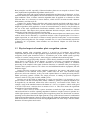
1.1 ANPR systems as a practical application of artificial intelligence
Massive integration of information technologies into all aspects of modern life caused demand
for processing vehicles as conceptual resources in information systems. Because a standalone
information system without any data has no sense, there was also a need to transform
information about vehicles between the reality and information systems. This can be achieved
by a human agent, or by special intelligent equipment which is be able to recognize vehicles by
their number plates in a real environment and reflect it into conceptual resources. Because of
this, various recognition techniques have been developed and number plate recognition systems
are today used in various traffic and security applications, such as parking, access and border
control, or tracking of stolen cars.
In parking, number plates are used to calculate duration of the parking. When a vehicle
enters an input gate, number plate is automatically recognized and stored in database. When a
vehicle later exits the parking area through an output gate, number plate is recognized again and
paired with the first-one stored in the database. The difference in time is used to calculate the
parking fee. Automatic number plate recognition systems can be used in access control. For
example, this technology is used in many companies to grant access only to vehicles of
authorized personnel.
In some countries, ANPR systems installed on country borders automatically detect and
monitor border crossings. Each vehicle can be registered in a central database and compared to a
black list of stolen vehicles. In traffic control, vehicles can be directed to different lanes for a
better congestion control in busy urban communications during the rush hours.
1.2 Mathematical aspects of number plate recognition systems
In most cases, vehicles are identified by their number plates, which are easily readable for
humans, but not for machines. For machine, a number plate is only a grey picture defined as a
two-dimensional function f ( x, y ) , where x and y are spatial coordinates, and f is a light
intensity at that point. Because of this, it is necessary to design robust mathematical machinery,
which will be able to extract semantics from spatial domain of the captured image. These
functions are implemented in so-called “ANPR systems”, where the acronym “ANPR” stands
for an “Automatic Number Plate Recognition”. ANPR system means transformation of data
between the real environment and information systems.
The design of ANPR systems is a field of research in artificial intelligence, machine vision,
pattern recognition and neural networks. Because of this, the main goal of this thesis is to study
algorithmic and mathematical principles of automatic number plate recognition systems.
Chapter two deals with problematic of number plate area detection. This problematic
includes algorithms, which are able to detect a rectangular area of the number plate in original
image. Humans define the number plate in a natural language as a “small plastic or metal plate
attached to a vehicle for official identification purposes”, but machines do not understand this
definition. Because of this, there is a need to find an alternative definition of the number plate
based on descriptors, which will be comprehensible for machines. This is a fundamental
problem of machine vision and of this chapter.
Chapter three describes principles of the character segmentation. In most cases, characters
are segmented using the horizontal projection of a pre-processed number plate, but sometimes
1
these principles can fail, especially if detected number plates are too warped or skewed. Then,
more sophisticated segmentation algorithms must be used.
Chapter four deals with various methods normalization and detection of characters. At first,
character dimensions and brightness must be normalized to ensure invariance towards a size and
light conditions. Then, a feature extraction algorithm must be applied on a character to filter
irrelevant data. It is necessary to extract features, which will be invariant towards character
deformations, used font style etc.
Chapter five studies pattern classifiers and neural networks and deals with their usage in
recognition of characters. Characters can be classified and recognized by the simple nearest
neighbor algorithm (1NN) applied to a vector of extracted features, or there is also possibility to
use one of the more sophisticated classification methods, such as feed-forward or Hopfield
neural networks. This chapter also presents additional heuristic analyses, which are used for
elimination of non-character elements from the plate.
Sometimes, the recognition process may fail and the detected plate can contain errors. Some
of these errors can be detected by a syntactical analysis of the recognized plate. If we have a
regular expression, or a rule how to evaluate a country-specific license plate, we can reconstruct
defective plates using this rule. For example, a number zero “0” can be automatically repaired to
a character “O” on positions, where numbers are not allowed. Chapter six deals with this
problematic.
1.3 Physical aspects of number plate recognition systems
Automatic number plate recognition system is a special set of hardware and software
components that proceeds an input graphical signal like static pictures or video sequences, and
recognizes license plate characters from it. A hardware part of the ANPR system typically
consists of a camera, image processor, camera trigger, communication and storage unit.
The hardware trigger physically controls a sensor directly installed in a lane. Whenever the
sensor detects a vehicle in a proper distance of camera, it activates a recognition mechanism.
Alternative to this solution is a software detection of an incoming vehicle, or continual
processing of the sampled video signal. Software detection, or continual video processing may
consume more system resources, but it does not need additional hardware equipment, like the
hardware trigger.
Image processor recognizes static snapshots captured by the camera, and returns a text
representation of the detected license plate. ANPR units can have own dedicated image
processors (all-in-one solution), or they can send captured data to a central processing unit for
further processing (generic ANPR). The image processor is running on special recognition
software, which is a key part of whole ANPR system.
Because one of the fields of application is a usage on road lanes, it is necessary to use a
special camera with the extremely short shutter. Otherwise, quality of captured snapshots will
be degraded by an undesired motion blur effect caused by a movement of the vehicle. For
example, usage of the standard camera with shutter of 1/100 sec to capture a vehicle with speed
of 80 km/h will cause a motion skew in amount of 0.22 m. This skew means the significant
degradation of recognition abilities.
There is also a need to ensure system invariance towards the light conditions. Normal
camera should not be used for capturing snapshots in darkness or night, because it operates in a
visible light spectrum. Automatic number plate recognition systems are often based on cameras
operating in an infrared band of the light spectrum. Usage of the infrared camera in combination
with an infrared illumination is better to achieve this goal. Under the illumination, plates that are
made from reflexive material are much more highlighted than rest of the image. This fact makes
detection of license plates much easier.
2
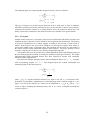
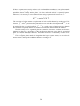
Figure 1.1: (a) Illumination makes detection of reflexive image plates easier. (b) Long
camera shutter and a movement of the vehicle can cause an undesired motion blur effect.
1.4 Notations and mathematical symbols
Logic symbols
p⊕q
p∧q
p∨q
¬p
Exclusive logical disjunction ( p xor q )
Logical conjunction ( p and q )
Logical disjunction ( p or q )
Exclusion ( not p )
Mathematical definition of image
f ( x, y )
x and y are spatial coordinates of an image, and f is an intensity of light at
that point. This function is always discrete on digital computers.
x ∈ ℕ 0 ∧ y ∈ ℕ 0 , where ℕ 0 denotes the set of natural numbers including
zero.
The intensity of light at point p . f ( p ) = f ( x, y ) , where p = [ x, y ]
f ( p)
Pixel neighborhoods
ɺɺ p
p1 N
4 2
ɺɺ
pN p
1
8
2
Pixel p1 is in a four-pixel neighborhood of pixel p2 (and vice versa)
Pixel p1 is in an eight-pixel neighborhood of pixel p2 (and vice versa)
Convolutions
a ( x) ∗ b( x)
a ( x) ∗ɶ b( x)
Discrete convolution of signals a ( x ) and b ( x )
Discrete periodical convolution of signals a ( x ) and b ( x )
3
Vectors and sets
m [ x, y ]
max A
The element in xth column and yth row of matrix m .
min A
mean A
median A
A
x
xi
The maximum value contained in the set A . The scope of elements can be
specified by additional conditions
The minimum value contained in the set A
The mean value of the elements contained in the set A
The median value of the elements contained in the set A
The cardinality of the set A . (Number of elements contained in the set)
Vectors or any other ordered sequences of numbers are printed bold.
The elements of vectors are denoted as xi , where i is a sequence number
x[a]
(starting with zero), such as i ∈ 0… n − 1 , where n = x is a cardinality of the
vector (number of elements)
The element a of the vector x . For example, the vector x can contain
x
(i )
elements a , b , c , d , such as x = ( a, b, c, d )
If there is more than one vector denoted as x , they are distinguished by their
indexes i . The upper index (i) does not mean the ith element of vector.
Intervals
a< x<b
x ∈ a… b
x lies in the interval between a and b . This notation is used when x is the
spatial coordinate in image (discrete as well as continuous)
This notation has the same meaning as the above one, but it is used when x is
a discrete sequence number.
Quantificators
∃x
∃! x
∃n x
¬∃x
∀x
There exists at least one x
There exists exactly one x
There exists exactly n x
There does not exist x
For every x
Rounding
x
x
Number x rounded down to the nearest integer
Number x rounded up to the nearest integer
4
Chapter 2
Principles of number plate
area detection
The first step in a process of automatic number plate recognition is a detection of a number plate
area. This problematic includes algorithms that are able to detect a rectangular area of the
number plate in an original image. Humans define a number plate in a natural language as a
“small plastic or metal plate attached to a vehicle for official identification purposes”, but
machines do not understand this definition as well as they do not understand what “vehicle”,
“road”, or whatever else is. Because of this, there is a need to find an alternative definition of a
number plate based on descriptors that will be comprehensible for machines.
Let us define the number plate as a “rectangular area with increased occurrence of
horizontal and vertical edges”. The high density of horizontal and vertical edges on a small area
is in many cases caused by contrast characters of a number plate, but not in every case. This
process can sometimes detect a wrong area that does not correspond to a number plate. Because
of this, we often detect several candidates for the plate by this algorithm, and then we choose
the best one by a further heuristic analysis.
Let an input snapshot be defined by a function f ( x, y ) , where x and y are spatial
coordinates, and f is an intensity of light at that point. This function is always discrete on
digital computers, such as x ∈ ℕ 0 ∧ y ∈ ℕ 0 , where ℕ 0 denotes the set of natural numbers
including zero. We define operations such as edge detection or rank filtering as mathematical
transformations of function f .
The detection of a number plate area consists of a series of convolve operations. Modified
snapshot is then projected into axes x and y . These projections are used to determine an area
of a number plate.
2.1 Edge detection and rank filtering
We can use a periodical convolution of the function f with specific types of matrices m to
detect various types of edges in an image:
w−1 h −1
f ′ ( x, y ) = f ( x, y ) ∗ɶ m [ x, y ] = ∑∑ f ( x, y ) ⋅ m mod w ( x − i ) , mod h ( y − j )
i =0 j =0
where w and h are dimensions of the image represented by the function f
Note: The expression m [ x, y ] represents the element in xth column and yth row of matrix m .
2.1.1
Convolution matrices
Each image operation (or filter) is defined by a convolution matrix. The convolution matrix
defines how the specific pixel is affected by neighboring pixels in the process of convolution.
5
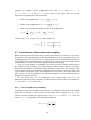
Individual cells in the matrix represent the neighbors related to the pixel situated in the centre of
the matrix. The pixel represented by the cell y in the destination image (fig. 2.1) is affected by
the pixels x0 … x8 according to the formula:
y = x0 × m0 + x1 × m1 + x2 × m2 + x3 × m3 + x4 × m4 + x5 × m5 + x6 × m6 + x7 × m7 + x8 × m8
Figure 2.1: The pixel is affected by its neighbors according to the convolution matrix.
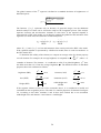
Horizontal and vertical edge detection
To detect horizontal and vertical edges, we convolve source image with matrices m he and m ve .
The convolution matrices are usually much smaller than the actual image. Also, we can use
bigger matrices to detect rougher edges.
−1 −1 −1
−1 0 1
m he = 0 0 0 ; m ve = −1 0 1
1 1 1
−1 0 1
Sobel edge detector
The Sobel edge detector uses a pair of 3x3 convolution matrices. The first is dedicated for
evaluation of vertical edges, and the second for evaluation of horizontal edges.
−1 −2 −1
−1 0 1
G x = 0 0 0 ; G y = −2 0 2
1 2 1
−1 0 1
The magnitude of the affected pixel is then calculated using the formula G = G 2x + G 2y . In
praxis, it is faster to calculate only an approximate magnitude as G = G x + G y .
Horizontal and vertical rank filtering
Horizontally and vertically oriented rank filters are often used to detect clusters of high density
of bright edges in the area of the number plate. The width of the horizontally oriented rank filter
matrix is much larger than the height of the matrix ( w ≫ h ), and vice versa for the vertical rank
filter ( w ≪ h ).
To preserve the global intensity of an image, it is necessary to each pixel be replaced with
an average pixel intensity in the area covered by the rank filter matrix. In general, the
convolution matrix should meet the following condition:
6
w −1 h −1
∑∑ m [i, j ] = 1.0
hr
i =0 j =0
where w and h are dimensions of the matrix.
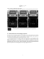
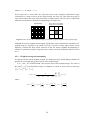
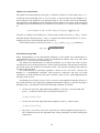
The following pictures show the results of application of the rank and edge detection filters.
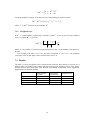
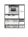
Figure 2.2: (a) Original image (b) Horizontal rank filter (c) Vertical rank filter (d)
Sobel edge detection (e) Horizontal edge detection (f) Vertical edge detection
2.2 Horizontal and vertical image projection
After the series of convolution operations, we can detect an area of the number plate according
to a statistics of the snapshot. There are various methods of statistical analysis. One of them is a
horizontal and vertical projection of an image into the axes x and y .
The vertical projection of the image is a graph, which represents an overall magnitude of the
image according to the axis y (see figure 2.3). If we compute the vertical projection of the
image after the application of the vertical edge detection filter, the magnitude of certain point
represents the occurrence of vertical edges at that point. Then, the vertical projection of so
transformed image can be used for a vertical localization of the number plate. The horizontal
projection represents an overall magnitude of the image mapped to the axis x .
7
Figure 2.3: Vertical projection of image to a y axis
Let an input image be defined by a discrete function f ( x, y ) . Then, a vertical projection p y of
the function f at a point y is a summary of all pixel magnitudes in the yth row of the input
image. Similarly, a horizontal projection at a point x of that function is a summary of all
magnitudes in the xth column.
We can mathematically define the horizontal and vertical projection as:
h −1
p x ( x ) = ∑ f ( x, j ) ;
j =0
w −1
p y ( y ) = ∑ f ( i, y )
i =0
where w and h are dimensions of the image.
2.3 Double-phase statistical image analysis
The statistical image analysis consists of two phases. The first phase covers the detection of a
wider area of the number plate. This area is then deskewed, and processed in the second phase
of analysis. The output of double-phase analysis is an exact area of the number plate. These two
phases are based on the same principle, but there are differences in coefficients, which are used
to determine boundaries of clipped areas.
The detection of the number plate area consists of a “band clipping” and a “plate clipping”.
The band clipping is an operation, which is used to detect and clip the vertical area of the
number plate (so-called band) by analysis of the vertical projection of the snapshot. The plate
clipping is a consequent operation, which is used to detect and clip the plate from the band (not
from the whole snapshot) by a horizontal analysis of such band.
Snapshot
Assume the snapshot is represented by a function f ( x, y ) , where x0 ≤ x ≤ x1 and y0 ≤ y ≤ y1 .
The [ x0 , y0 ] represents the upper left corner of the snapshot, and [ x1 , y1 ] represents the bottom
right corner. If w and h are dimensions of the snapshot, then x0 = 0 , y0 = 0 , x1 = w − 1 and
y1 = h − 1 .
8
Band
The band b in the snapshot f is an arbitrary rectangle b = ( xb 0 , yb 0 , xb1 , yb1 ) , such as:
( xb 0 = xmin ) ∧ ( xb1 = xmax ) ∧ ( ymin ≤ yb0 < yb1 ∧ ymax )
Plate
(
)
Similarly, the plate p in the band b is an arbitrary rectangle p = x p 0 , y p 0 , x p1 , y p1 , such as:
(x
b0
) (
) (
≤ x p 0 ≤ x p1 ≤ xb1 ∧ y p 0 = yb 0 ∧ y p 0 = yb 0
)
The band can be also defined as a vertical selection of the snapshot, and the plate as a horizontal
selection of the band. The figure 2.4 schematically demonstrates this concept:
yb 0
x p0
x p1
yb1
Figure 2.4: The double-phase plate clipping. Black color represents the first phase of plate clipping,
and red color represents the second one. Bands are represented by dashed lines, and plates by solid
lines.
2.3.1
Vertical detection – band clipping
The first and second phase of band clipping is based on the same principle. The band clipping is
a vertical selection of the snapshot according to the analysis of a graph of vertical projection. If
h is the height of the analyzed image, the corresponding vertical projection p yr ( y ) contains h
values, such as y ∈ 0; h − 1 .
The graph of projection may be sometimes too “ragged” for analysis due to a big statistical
dispersion of values p yr ( y ) . There are two approaches how to solve this problem. We can blur
the source snapshot (costly solution), or we can decrease the statistical dispersion of the ragged
projection p ry by convolving its projection with a rank vector:
ɶ hr [ y ]
p y ( y ) = p yr ( y ) ∗m
where m hr is the rank vector (analogous to the horizontal rank matrix in section 2.1.1). The
width of the vector m hr is nine in default configuration.
After convolution with the rank vector, the vertical projection of the snapshot in figure 2.3
can look like this:
9
py ( y )
yb 0 ybm yb1
100%
0%
y
y0
y1
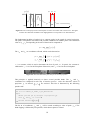
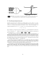
Figure 2.5: The vertical projection of the snapshot 2.3 after convolution with a rank vector. The figure
contains three detected candidates. Each highlighted area corresponds to one detected band.
The fundamental problem of analysis is to compute peaks in the graph of vertical projection.
The peaks correspond to the bands with possible candidates for number plates. The maximum
value of p y ( y ) corresponding to the axle of band can be computed as:
ybm = arg max
y0 ≤ y ≤ y1
{ p ( y )}
y
The yb 0 and yb1 are coordinates of band, which can be detected as:
yb 0 = max
y0 ≤ y ≤ ybm
yb1 = min
ybm ≤ y ≤ y1
{ y p ( y ) ≤ c ⋅ p ( y )}
{ y p ( y ) ≤ c ⋅ p ( y )}
y
y
y
bm
y
y
y
bm
c y is a constant, which is used to determine the foot of peak ybm . In praxis, the constant is
calibrated to c1 = 0.55 for the first phase of detection, and c2 = 0.42 for the second phase.
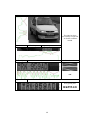
Figure 2.6: The band detected by the analysis of vertical projection
This principle is applied iteratively to detect several possible bands. The yb 0 and yb1
coordinates are computed in each step of iterative process. After the detection, values of
projection p y in interval yb 0 , yb1 are zeroized. This idea is illustrated by the following
pseudo-code:
let L to be a list of detected candidates
for i :=0 to number_of_bands_to_be_detected do
begin
detect
save
yb 0 and yb1 by analysis of projection p y
yb 0 and yb1 to a list L
zeroize interval
yb 0 , yb1
end
The list L of coordinates yb 0 and yb1 will be sorted according to value of peak ( ybm ). The
band clipping is followed by an operation, which detects plates in a band.
10
2.3.2
Horizontal detection – plate clipping
In contrast with the band clipping, there is a difference between the first and second phase of
plate clipping.
First phase
There is a strong analogy in a principle between the band and plate clipping. The plate clipping
is based on a horizontal projection of band. At first, the band must be processed by a vertical
detection filter. If w is a width of the band (or a width of the analyzed image), the
corresponding horizontal projection pxr ( x ) contains w values:
px ( x ) =
yb1
∑ f ( x, j )
j = yb 0
Please notice that px ( x ) is a projection of the band, not of the whole image. This can be
achieved by a summation in interval yb 0 , yb1 , which represents the vertical boundaries of the
band. Since the horizontal projection pxr ( x ) may have a big statistical dispersion, we decrease
it by convolving with a rank vector ( px ( x ) = pxr ( x ) ⊻ɶ mvr [ x ] ). The width of the rank vector is
usually equal to a half of an estimated width of the number plate.
Then, the maximum value corresponding to the plate can be computed as:
xbm = arg max { px ( x )}
x0 ≤ y ≤ x1
The xb 0 and xb1 are coordinates of the plate, which can be then detected as:
xb 0 = max
{x p ( x ) ≤ c ⋅ p ( x )}
{x p ( x ) ≤ c ⋅ p ( x )}
x0 ≤ x ≤ xbm
xb1 = min
xbm ≤ x≤ x1
x
x
x
bm
x
x
x
bm
where cx is a constant, which is used to determine the foot of peak xbm . The constant is
calibrated to cx = 0.86 for the first phase of detection.
Second phase
In the second phase of detection, the horizontal position of a number plate is detected in another
way. Due to the skew correction between the first and second phase of analysis, the wider plate
area must be duplicated into a new bitmap. Let f n ( x, y ) be a corresponding function of such
bitmap. This picture has a new coordinate system, such as [0,0] represents the upper left corner
and [ w − 1, h − 1] the bottom right, where w and h are dimensions of the area. The wider area of
the number plate after deskewing is illustrated in figure 2.8.
In contrast with the first phase of detection, the source plate has not been processed by the
vertical detection filter. If we assume that plate is white with black borders, we can detect that
borders as black-to-white and white-to-black transitions in the plate. The horizontal projection
px ( x ) of the image is illustrated in the figure 2.7.a. To detect the black-to-white and white-toblack transitions, there is a need to compute a derivative p′x ( x ) of the projection px ( x ) . Since
the projection is not continuous, the derivation step cannot be an infinitely small number
11
( h ≠ lim x ). If we derive a discrete function, the derivation step h must be an integral number
x→0
(for example h = 4 ). Let the derivative of px ( x ) be defined as:
p x′ ( x ) =
p x ( x ) − px ( x − h )
h
Where h = 4 .
px ( x )
100%
0%
w −1
x
p′x ( x )
0
w −1
Figure 2.7: (a) The horizontal projection
of
x
px ( x ) of the plate in figure 2.8. (b) The derivative
px ( x ) . Arrows denote the “BW” and “WB” transitions, which are used to determine the
boundaries of the plate.
Figure 2.8: The wider area of the number plate after deskewing.
The left and right boundary of the plate can be determined by an analysis of the projection
p′x ( x ) . The left corner x p 0 is represented by the black-to-white transition (positive peak in
figure 2.7.b), and right corner x p1 by the white-to-black transition (negative peak in figure
2.7.b):
{
0≤ x< w
{
0≤ x < w
{
}}
x p 0 = min x px′ ( x ) ≥ cd ⋅ max px′ ( x )
0≤ x<
w
2
}
x p1 = max x p′x ( x ) ≤ cd ⋅ min { p′x ( x )}
w
≤ x<w
2
where cd is a constant used to determine the most left negative and the most right positive peak.
The left and right corners must lie on the opposite halves of the detected plate according to the
w
w
constraints 0 ≤ x < for x p 0 , and ≤ x < w for x p1 .
2
2
12
In this phase of the recognition process, it is not possible to select a best candidate for a
number plate. This can be done by a heuristic analysis of characters after the segmentation.
2.4 Heuristic analysis and priority selection of number plate
candidates
In general, the captured snapshot can contain several number plate candidates. Because of this,
the detection algorithm always clips several bands, and several plates from each band. There is a
predefined value of maximum number of candidates, which are detected by analysis of
projections. By default, this value is equals to nine.
There are several heuristics, which are used to determine the cost of selected candidates
according to their properties. These heuristics have been chosen ad hoc during the practical
experimentations. The recognition logic sorts candidates according to their cost from the most
suitable to the least suitable. Then, the most suitable candidate is examined by a deeper heuristic
analysis. The deeper analysis definitely accepts, or rejects the candidate. As there is a need to
analyze individual characters, this type of analysis consumes big amount of processor time.
The basic concept of analysis can be illustrated by the following steps:
1.
2.
3.
4.
5.
2.4.1
Detect possible number plate candidates.
Sort them according to their cost (determined by a basic heuristics).
Cut the first plate from the list with the best cost.
Segment and analyze it by a deeper analysis (time consuming).
If the deeper analysis refuses the plate, return to the step 3.
Priority selection and basic heuristic analysis of bands
The basic analysis is used to evaluate the cost of candidates, and to sort them according to this
cost. There are several independent heuristics, which can be used to evaluate the cost α i . The
heuristics can be used separately, or they can be combined together to compute an overall cost
of candidate by a weighted sum:
α = 0.15 ⋅ α1 + 0.25 ⋅ α 2 + 0.4 ⋅ α 3 + 0.4 ⋅ α 4
Heuristics
α1 = yb 0 − yb1
α2 =
α3 =
Illustration
Description
The height of band in pixels. Bands
with a lower height will be preferred.
p y ( ybm )
1
p y ( ybm )
peak of vertical projection of snapshot,
which corresponds to the processed
band. Bands with a higher amount of
vertical edges will be preferred.
This heuristics is similar to the previous
one, but it considers not only the value
of the greatest peak, but a value of area
under the graph between points yb 0 and
yb1 . These points define a vertical
position of the evaluated band.
1
yb1
∑ p ( y)
y
y = yb 0
The “ p y ( ybm ) ” is a maximum value of
yb1
yb 0
∑
13
α4 =
2.4.2
x p 0 − x p1
yb 0 − yb1
The proportions of the one-row number
plates are similar in the most countries.
If we assume that width/height ratio of
the plate is about five, we can compare
the measured ratio with the estimated
one to evaluate the cost of the number
plate.
−5
Deeper analysis
The deeper analysis determines the validity of a candidate for the number plate. Number plate
candidates must be segmented into the individual characters to extract substantial features. The
list of candidates is iteratively processed until the first valid number plate is found. The
candidate is considered as a valid number plate, if it meets the requirements for validity.
Assume that plate p is segmented into several characters p0 … pn −1 , where n is a number
of characters. Let wi be a width of ith character (see figure 2.9.a). Since all segmented
characters have roughly uniform width, we can use a standard deviation of these values as a
heuristics:
β1 =
1
n
n −1
∑ ( w − w)
2
i
i =0
1 n −1
wi .
n i=0
If we assume that the number plate consists of dark characters on a light background, we
can use a brightness histogram to determine if the candidate meets this condition. Because some
country-specific plates are negative, we can use the histogram to deal with this type of plates
(see figure 2.9.b).
Let H ( b ) be a brightness histogram, where b is a certain brightness value. Let bmin and
where w is an arithmetic average of character widths w =
∑
bmax be a value of a darkest and lightest point. Then, H ( b ) is a count of pixels, whose values
are equal to b . The plate is negative when the heuristics β 2 is negative:
bmax
bmid
β2 =
H (b) −
H (b)
b =b
mid
b =bmin
∑
∑
where bmid is a middle point in the histogram, such as bmid =
14
bmax − bmin
.
2
p0
p1
p2
p3
p4
p5
p6
p7
p8
p9
w ( p2 )
H (b )
bmin
bmid
bmax
Pixel numbers
b
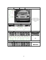
Figure 2.9: (a) The number plate must be segmented into individual characters for deeper
heuristic analysis. (b) Brightness histogram of the number plate is used to determine the
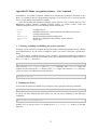
positivity of the number plate.
2.5 Deskewing mechanism
The captured rectangular plate can be rotated and skewed in many ways due to the positioning
of vehicle towards the camera. Since the skew significantly degrades the recognition abilities, it
is important to implement additional mechanisms, which are able to detect and correct skewed
plates.
The fundamental problem of this mechanism is to determine an angle, under which the plate
is skewed. Then, deskewing of so evaluated plate can be realized by a trivial affine
transformation.
It is important to understand the difference between the “sheared” and “rotated” rectangular
plate. The number plate is an object in three-dimensional space, which is projected into the twodimensional snapshot during the capture. The positioning of the object can sometimes cause the
skew of angles and proportions.
If the vertical line of plate v p is not identical to the vertical line of camera objective vc , the
plate may be sheared. If the vertical lines v p and vc are identical, but the axis a p of plate is not
parallel to the axis of camera ac , the plate may be rotated. (see figure 2.10)
15
ap
ap
ap
vp
vc = v p
vc = v p
a p ac ∧ v p = vc
ac
vc
a p ac ∧ v p = vc
ac
a p ac ∧ v p ≠ vc
ac
Figure 2.10: (a) Number plate captured under the right angle (b) rotated plate (c)
Sheared plate
2.5.1
Detection of skew
Hough transform is a special operation, which is used to extract features of a specific shape
within a picture. The classical Hough transform is used for the detection of lines. The Hough
transform is widely used for miscellaneous purposes in the problematic of machine vision, but I
have used it to detect the skew of captured plate, and also to compute an angle of skew.
It is important to know, that Hough transform does not distinguish between the concepts
such as “rotation” and “shear”. The Hough transform can be used only to compute an
approximate angle of image in a two-dimensional domain.
The mathematical representation of line in the orthogonal coordinate system is an equation
y = a ⋅ x + b , where a is a slope and b is a y-axis section of so defined line. Then, the line is a
set of all points [ x, y ] , for which this equation is valid. We know that the line contains an
infinite number of points as well as there are an infinite number of different lines, which can
cross a certain point. The relation between these two assertions is a basic idea of the Hough
transform.
The equation y = a ⋅ x + b can be also written as b = − x ⋅ a + y , where x and y are
parameters. Then, the equation defines a set of all lines (a, b) , which can cross the point [ x, y ] .
For each point in the “XY” coordinate system, there is a line in an “AB” coordinate system (so
called “Hough space”)
y
b
[ x0 , y0 ]
b = x0 ⋅ a + y0
m
k
l
m
l
k
x
a
Figure 2.11: The “XY” and “AB” (“Hough space”) coordinate systems. Each point [ x0 , y0 ] in the
“XY” coordinate system corresponds to one line in the Hough space (red color). The are several points
(marked as k , l , m ) in the Hough space, that correspond to the lines in the “XY” coordinate system,
which can cross the point. [ x0 , y0 ] .
16
Let f ( x, y ) be a continuous function. For each point [ a, b ] in Hough space, there is a line in
the “XY” coordinate system. We compute a magnitude of point [ a, b ] as a summary of all
points in the “XY” space, which lie on the line a ⋅ x + b .
Assume that f ( x, y ) is a discrete function, which represents the snapshot with definite
dimensions ( w × h) . To compute the Hough transform of the function like this, it is necessary to
normalize it into a unified coordinate system in the following way:
x′ =
2⋅ x
2⋅ y
− 1 ; y′ =
−1
w
h
Although the space defined by a unified coordinate system is always discrete (floating point) on
digital computers, we will assume that it is continuous. Generally, we can define the Hough
transform h′ ( a′, b′ ) of a continuous function f ′ ( x′, y ′ ) in the unified coordinate system as:
h′ ( a′, b′ ) =
1
∫ f ′ ( x′, a′ ⋅ x′ + b′)dx′
−1
x′
−
π
0
2
π
θ
−∞
0
−∞
a′
2
y′
b′
b′
Figure 2.12: (a) Number plate in the unified “ XY ” coordinate system after application
of the horizontal edge detection filter (b) Hough transform of the number plate in the
“ θ B ” coordinate system (c) Colored Hough transform in the “ AB ” coordinate system.
We use the Hough transform of certain image to evaluate its skew angle. You can see the
colored Hough transform on the figure 2.12.c. The pixels with a relatively high value are
marked by a red color. Each such pixel corresponds to a long white line in the figure 13.a. If we
assume that the angle of such lines determines the overall angle, we can find the longest line as:
( am′ , bm′ ) = arg 0max
{h′ ( a′, b′)}
≤ a′≤1
0 ≤ b′≤1
To compute the angle of such a line, there is a need to transform it back to the original
coordinate system:
[ am , bm ] = w ⋅
am′ − 1
b′ − 1
,h ⋅ m
2
2
where w and h are dimensions of the evaluated image. Then, the overall angle θ of image can
be computed as:
θ = arctan ( am )
17
The more sophisticated solution is to determine the angle from a horizontal projection of the
Hough transform h′ . This approach is much better because it covers all parallel lines together,
not only the longest one:
θˆ = arctan w ⋅
aˆm′ − 1
; aˆm′ = arg max { pa′ ( a′ )}
−1≤ a ′≤1
2
where pa′ ( a′ ) is a horizontal projection of the Hough space, such as:
pa′ ( a′ ) =
1
∫ f ′ ( a′, b′)db′
−1
2.5.2
Correction of skew
The second step of a deskewing mechanism is a geometric operation over an image f ( x, y ) . As
the skew detection based on Hough transform does not distinguish between the shear and
rotation, it is important to choose the proper deskewing operation. In praxis, plates are sheared
in more cases than rotated. To correct the plate sheared by the angle θ , we use the affine
transformation to shear it by the negative angle −θ .
For this transformation, we define a transformation matrix A :
1
A = S x
0
Sy
1
0
0 1 − tan (θ ) 0
0 = 0
1
0
1 0
0
1
where S x and S y are shear factors. The S x is always zero, because we shear the plate only in a
direction of the Y-axis.
Let P be a vector representing the certain point, such as P = [ x, y,1] where x and y are
coordinates of that point. The new coordinates Ps = [ xs , ys ,1] of that point after the shearing can
be computed as:
Ps = P ⋅ A
where A is a corresponding transformation matrix.
Let the deskewed number plate be defined by a function f s . The function f s can be
computed in the following way:
f s ( x, y ) = f
([ x, y,1] ⋅ A ⋅ [1,0,0] ,[ x, y,1] ⋅ A ⋅ [0,1,0] )
T
T
After the substitution of the transformation matrix A :
1 − tan (θ ) 0 1
f s ( x, y ) = f [ x, y,1] ⋅ 0
1
0 ⋅ 0 ,
0
0
1 0
18
1 − tan (θ ) 0 0
1
0 ⋅ 1
[ x, y,1] ⋅ 0
0
0
1 0
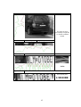
Figure 2.13: (a) Original number plate. (b) Number plate after deskewing.
19
Chapter 3
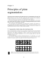
Principles of plate
segmentation
The next step after the detection of the number plate area is a segmentation of the plate. The
segmentation is one of the most important processes in the automatic number plate recognition,
because all further steps rely on it. If the segmentation fails, a character can be improperly
divided into two pieces, or two characters can be improperly merged together.
We can use a horizontal projection of a number plate for the segmentation, or one of the
more sophisticated methods, such as segmentation using the neural networks. If we assume
only one-row plates, the segmentation is a process of finding horizontal boundaries between
characters. Section 3.2 deals with this problematic.
The second phase of the segmentation is an enhancement of segments. The segment of a
plate contains besides the character also undesirable elements such as dots and stretches as well
as redundant space on the sides of character. There is a need to eliminate these elements and
extract only the character. Section 3.3 deals with these problems.
3.1 Segmentation of plate using a horizontal projection
Since the segmented plate is deskewed, we can segment it by detecting spaces in its horizontal
projection. We often apply the adaptive thresholding filter to enhance an area of the plate before
segmentation. The adaptive thresholding is used to separate dark foreground from light
background with non-uniform illumination. You can see the number plate area after the
thresholding in figure 3.1.a.
After the thresholding, we compute a horizontal projection px ( x ) of the plate f ( x, y ) . We
use this projection to determine horizontal boundaries between segmented characters. These
boundaries correspond to peaks in the graph of the horizontal projection (figure 3.1.b).
y
x
px ( x )
vm
va
vb
x
Figure 3.1: (a) Number plate after application of the adaptive thresholding (b) Horizontal
projection of plate with detected peaks. Detected peaks are denoted by dotted vertical lines.
20
The goal of the segmentation algorithm is to find peaks, which correspond to the spaces
between characters. At first, there is a need to define several important values in a graph of the
horizontal projection px ( x ) :
•
vm - The maximum value contained in the horizontal projection px ( x ) , such as
vm = max { px ( x )} , where w is a width of the plate in pixels.
0≤ x < w
•
•
1 w−1
px ( x )
w x =0
vb - This value is used as a base for evaluation of peak height. The base value is
always calculated as vb = 2 ⋅ va − vm . The va must lie on vertical axis between the values
vb and vm .
va - The average value of horizontal projection px ( x ) , such as va =
∑
The algorithm of segmentation iteratively finds the maximum peak in the graph of vertical
projection. The peak is treated as a space between characters, if it meets some additional
conditions, such as height of peak. The algorithm then zeroizes the peak and iteratively repeats
this process until no further space is found. This principle can be illustrated by the following
steps:
1. Determine the index of the maximum value of horizontal projection:
xm = arg max { px ( x )}
0≤ x < w
2. Detect the left and right foot of the peak as:
{
min { x p
}
)}
xl = max x px ( x ) ≤ cx ⋅ p x ( xm )
0 ≤ x ≤ xm
xr =
xm ≤ x < w
x
( x ) ≤ cx ⋅ px ( xm
3. Zeroize the horizontal projection px ( x ) on interval xl , xr
4. If px ( xm ) < cw ⋅ vm , go to step 7.
5. Divide the plate horizontally in the point xm .
6. Go to step 1.
7. End.
Two different constants have been used in the algorithm above. The constant cx is used to
determine foots of peak xm . The optimal value of cx is 0.7.
The constant cw determines the minimum height of the peak related to the maximum value
of the projection ( vm ). If the height of the peak is below this minimum, the peak will not be
considered as a space between characters. It is important to choose a value of constant cw
carefully. An inadequate small value causes that too many peaks will be treated as spaces, and
characters will be improperly divided. A big value of cw causes that not all regular peaks will
be treated as spaces, and characters will be improperly merged together. The optimal value of
cw is 0.86. To ensure a proper behavior of the algorithm, constants cx and cw should meet the
following condition:
∀ ( xl , xm , xr ) ∈ P : cw ⋅ vm > px ( xl ) ∧ px ( xr )
where P is a set of all detected peaks xm with corresponding foots xl and xr .
21
3.2 Extraction of characters from horizontal segments
The segment of plate contains besides the character also redundant space and other undesirable
elements. We understand under the term “segment” the part of a number plate determined by a
horizontal segmentation algorithm. Since the segment has been processed by an adaptive
thresholding filter, it contains only black and white pixels. The neighboring pixels are grouped
together into larger pieces, and one of them is a character. Our goal is to divide the segment into
the several pieces, and keep only one piece representing the regular character. This concept is
illustrated in figure 3.2.
Piece 1
Horizontal
segment
Piece 2
Piece 3
Piece 4
Figure 3.2: Horizontal segment of the number plate contains several groups (pieces) of neighboring
pixels.
3.2.1
Piece extraction
Let the segment be defined by a discrete function f ( x, y ) in the relative coordinate system,
such as [ 0,0] is an upper left corner of the segment, and [ w − 1, h − 1] is a bottom right corner,
where w and h are dimensions of the segment. The value of f ( x, y ) is “1” for the black
pixels, and “0” for the white space.
The piece Ρ is a set of all neighboring pixels [ x, y ] , which represents a continuous element.
The pixel [ x, y ] belongs to the piece Ρ if there is at least one pixel [ x′, y′] from the Ρ , such as
[ x, y ]
and [ x′, y′] are neighbors:
[ x, y ] ∈ Ρ ⇔ ∃[ x′, y′] ∈ Ρ : [ x, y ] Nɺɺ 4 [ x′, y′]
ɺɺ b means a binary relation “ a is a neighbor of b in a four-pixel
The notation aN
4
neighborhood”:
[ x, y ] Nɺɺ 4 [ x′, y′] ⇔
x − x′ = 1 ⊕ y − y ′ = 1
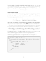
Algorithm
The goal of the piece extraction algorithm is to find and extract pieces from a segment of the
plate. This algorithm is based on a similar principle as a commonly known “seed-fill”
algorithm.
22
•
Let piece Ρ be a set of (neighboring) pixels [ x, y ]
•
Let S be a set of all pieces Ρ from a processed segment defined by the function
f ( x, y ) .
•
Let X be a set of all black pixels: X = [ x, y ] f ( x, y ) = 1
•
Let A be an auxiliary set of pixels
{
}
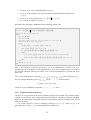
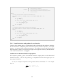
Principle of the algorithm is illustrated by the following pseudo-code:
let set
let set
S = 0/
{
}
X = [ x, y ] f ( x, y ) = 1 ∧ [ 0,0] ≤ [ x, y ] < [ w, h ]
while set X is not empty do
begin
let set Ρ = 0/
let set A = 0/
pull one pixel from set X and insert it into set
while set A is not empty do
begin
let
[ x, y ]
be a certain pixel from
A
A
[ x, y ] from a set A
f ( x, y ) = 1 ∧ [ x, y ] ∉ A ∧ [ 0,0] ≤ [ x, y ] < [ w, h ]
pull pixel
if
begin
then
[ x, y ] from set A and insert it into set Ρ
pixels [ x − 1, y ] , [ x + 1, y ] , [ x, y − 1] , [ x, y + 1] into set
pull pixel
insert
A
end
end
add
Ρ to set S
end
Note 1: The operation “pull one pixel from a set” is non-deterministic, because a set is an
unordered group of elements. In real implementation, a set will be implemented as an ordered
list, and the operation “pull one pixel from a set” will be implemented as “pull the first pixel
from a list”
Note 2: The mathematical conclusion [ xmin , ymin ] < [ x, y ] < [ xmax , ymax ] means “The pixel [ x, y ]
lies in a rectangle defined by pixels [ xmin , ymin ] and [ xmax , ymax ] ”. More formally:
[ x, y ]R[ x′, y′] ⇔ xRx′ ∧ yRy′
where R is a one of the binary relations: ‘ < ’, ’ > ’, ’ ≤ ’, ’ ≥ ’ and ’ = ’.
3.2.2
Heuristic analysis of pieces
The piece is a set of pixels in the local coordinate system of the segment. The segment usually
contains several pieces. One of them represents the character and others represent redundant
elements, which should be eliminated. The goal of the heuristic analysis is to find a piece, which
represents character.
Let us place the piece Ρ into an imaginary rectangle ( x0 , y0 , x1 , y1 ) , where [ x0 , y0 ] is an
upper left corner, and [ x1 , y1 ] is a bottom right corner of the piece:
23
x0 = min { x [ x, y ] ∈ Ρ}
x1 = max { x [ x, y ] ∈ Ρ}
y0 = min { y [ x, y ] ∈ Ρ}
y1 = max { y [ x, y ] ∈ Ρ}
The dimensions and area of the imaginary rectangle are defined as w = x0 − x1 , h = y0 − y1 and
S = w ⋅ h . Cardinality of the set Ρ represents the number of black pixels nb . The number of
white pixels nw can be then computed as nw = S − nb = w ⋅ h − Ρ . The overall magnitude M of a
piece is a ratio between the number of black pixels nb and the area S of an imaginary rectangle
M = nb / S .
In praxis, we use the number of white pixels nw as a heuristics. Pieces with a higher value
of nw will be preferred.
The piece chosen by the heuristics is then converted to a monochrome bitmap image. Each
such image corresponds to one horizontal segment. These images are considered as an output of
the segmentation phase of the ANPR process (see figure 3.3)
Figure 3.3: The input (a) and output (b) example of the segmentation phase of the ANPR
recognition process.
24
Chapter 4
Feature extraction and
normalization of characters
To recognize a character from a bitmap representation, there is a need to extract feature
descriptors of such bitmap. As an extraction method significantly affects the quality of whole
OCR process, it is very important to extract features, which will be invariant towards the
various light conditions, used font type and deformations of characters caused by a skew of the
image.
The first step is a normalization of a brightness and contrast of processed image segments.
The characters contained in the image segments must be then resized to uniform dimensions
(second step). After that, the feature extraction algorithm extracts appropriate descriptors from
the normalized characters (third step). This chapter deals with various methods used in the
process of normalization.
4.1 Normalization of brightness and contrast
The brightness and contrast characteristics of segmented characters are varying due to different
light conditions during the capture. Because of this, it is necessary to normalize them. There are
many different ways, but this section describes the three most used: histogram normalization,
global and adaptive thresholding.
Through the histogram normalization, the intensities of character segments are redistributed on the histogram to obtain the normalized statistics.
Techniques of the global and adaptive thresholding are used to obtain monochrome
representations of processed character segments. The monochrome (or black & white)
representation of image is more appropriate for analysis, because it defines clear boundaries of
contained characters.
4.1.1
Histogram normalization
The histogram normalization is a method used to re-distribute intensities on the histogram of the
character segments. The areas of lower contrast will gain a higher contrast without affecting the
global characteristic of image.
Consider a grayscale image defined by a discrete function f ( x, y ) . Let I be a total number
of gray levels in the image (for example I = 256 ). We use a histogram to determine the number
of occurrences of each gray level i , i ∈ 0… I − 1 :
H (i ) =
{[ x, y ] 0 ≤ x < w ∧ 0 ≤ y < h ∧ f ( x, y ) = i}
The minimum, maximum and average value contained in the histogram is defined as:
H min = min { f ( x, y )} ; H max = max { f ( x, y )} ; H avg =
0≤ x < w
0≤ y < h
0≤ x < w
0≤ y < h
25
1 w−1 h −1
f ( x, y )
w ⋅ h x =0 y =0
∑∑
where the values H min , H max and H avg are in the following relation:
0 ≤ H min ≤ H avg ≤ H max ≤ I − 1
The goal of the histogram normalization is to obtain an image with normalized statistical
I
characteristics, such as H min = 0 , H max = I − 1 , H avg = . To meet this goal, we construct a
2
transformation function g ( i ) as a Lagrange polynomial with interpolation points
[ x1 , y1 ] = [ H min ,0] , [ x2 , y2 ] = H avg ,
I
and [ x3 , y3 ] = [ H max , I − 1] :
2
3
i − xk
g (i ) = y j
j =1
k =1 x j − xk
k≠ j
3
∑ ∏
This transformation function can be explicitly written as:
g ( i ) = y1 ⋅
i − x2 i − x3
i − x1 i − x3
i − x1 i − x2
⋅
+ y2 ⋅
⋅
+ y3 ⋅
⋅
x1 − x2 x1 − x3
x2 − x1 x2 − x3
x3 − x1 x3 − x2
After substitution of concrete points, and concrete number of gray levels I = 256 :
g ( i ) = +128 ⋅
i − H avg
i − H max
i − H min
i − H min
⋅
+ 255 ⋅
⋅
H avg − H min H avg − H max
H max − H min H max − H avg
g (i )
I −1
I
2
i
0
H min
H avg
H max
brightness before transformation
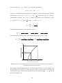
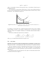
Figure 4.1: We use the Lagrange interpolating polynomial as a transformation function to normalize
the brightness and contrast of characters.
The Lagrange interpolating polynomial as a transformation function is a costly solution. It is
like harvesting one potato by a tractor. In praxis, there is more useful to construct the
transformation using a simple linear function that spreads the interval H min , H max into the
unified interval 0, I − 1 :
26
g (i ) =
i − H min
( I − 1)
H max − H min
The normalization of image is proceeded by the transformation function in the following way:
f n ( x, y ) = g ( f ( x, y ) )
4.1.2
Global Thresholding
The global thresholding is an operation, when a continuous gray scale of an image is reduced
into monochrome black & white colors according to the global threshold value. Let 0,1 be a
gray scale of such image. If a value of a certain pixel is above the threshold t , the new value of
the pixel will be zero. Otherwise, the new value will be one for pixels with values above the
threshold t .
Let v be an original value of the pixel, such as v ∈ 0,1 . The new value v′ is computed as:
0 if
v′ =
1 if
v ∈ 0, t )
v ∈ t ,1
The threshold value t can be obtained by using a heuristic approach, based on a visual
inspection of the histogram. We use the following algorithm to determine the value of t
automatically:
1. Select an initial estimate for threshold t (for example t = 0.5 )
{
}
2. The threshold t divides the pixels into the two different sets: Sa = [ x, y ] f ( x, y ) < t ,
{
}
and Sb = [ x, y ] f ( x, y ) ≥ t .
3. Compute the average gray level values µa and µb for the pixels in sets Sa and Sb as:
1
1
µa =
f ( x , y ) ; µb =
f ( x, y )
S a [ x , y ]∈Sa
Sb [ x , y ]∈Sb
∑
∑
1
( µ a + µb )
2
5. Repeat steps 2, 3, 4 until the difference △t in successive iterations is smaller than
predefined precision t p
4. Compute a new threshold value t =
Since the threshold t is global for a whole image, the global thresholding can sometimes fail.
Figure 4.2.a shows a partially shadowed number plate. If we compute the threshold t using the
algorithm above, all pixels in a shadowed part will be below this threshold and all other pixels
will be above this threshold. This causes an undesired result illustrated in figure 4.2.b.
27
H (b)
t
Pixel numbers
b
B
A
C
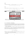
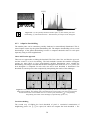
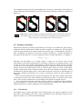
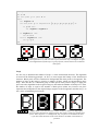
4.1.3
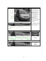
Figure 4.2: (a) The partially shadowed number plate. (b) The number plate after
thresholding. (c) The threshold value t determined by an analysis of the histogram.
Adaptive thresholding
The number plate can be sometimes partially shadowed or nonuniformly illuminated. This is
most frequent reason why the global thresholding fail. The adaptive thresholding solves several
disadvantages of the global thresholding, because it computes threshold value for each pixel
separately using its local neighborhood.
Chow and Kaneko approach
There are two approaches to finding the threshold. The first is the Chow and Kaneko approach,
and the second is a local thresholding. The both methods assumes that smaller rectangular
regions are more likely to have approximately uniform illumination, more suitable for
thresholding. The image is divided into uniform rectangular areas with size of m × n pixels. The
local histogram is computed for each such area and a local threshold is determined. The
threshold of concrete point is then computed by interpolating the results of the subimages.
1
2
3
5
6
?
4
Figure 4.3: The number plate (from figure 4.2) processed by the Chow and Kaneko approach of the
adaptive thresholding. The number plate is divided into the several areas, each with own histogram
and threshold value. The threshold value of a concrete pixel (denoted by ) is computed by
interpolating the results of the subimages (represented by pixels 1-6).
Local thresholding
The second way of finding the local threshold of pixel is a statistical examination of
neighboring pixels. Let [ x, y ] be a pixel, for which we compute the local threshold t . For
28
simplicity we condider a square neighborhood with width 2 ⋅ r + 1 , where
[ x − r, y + r ] , [ x + r, y − r ]
[ x − r, y − r ] ,
and [ x + r , y + r ] are corners of such square. There are severals
approaches of computing the value of threshold:
{ f ( i, j )}
•
Mean of the neighborhood : t ( x, y ) = mean
•
Median of the neighborhood : t ( x, y ) = median { f ( i, j )}
•
Mean of the minimum and maximum value of the heighborhood:
1
t ( x, y ) = min { f ( i, j )} + max { f ( i, j )}
x − r ≤i ≤ x + r
2 xy−−rr≤≤ij≤≤xy++rr
y −r ≤ j ≤ y + r
x − r ≤i ≤ x + r
y −r ≤ j≤ y + r
x − r ≤i ≤ x + r
y −r ≤ j≤ y + r
The new value f ′ ( x, y ) of pixel [ x, y ] is then computes as:
0 if
f ′ ( x, y ) =
1 if
f ( x, y ) ∈ 0, t ( x, y ) )
f ( x, y ) ∈ 0, t ( x, y )
4.2 Normalization of dimensions and resampling
Before extracting feature descriptors from a bitmap representation of a character, it is necessary
to normalize it into unified dimensions. We understand under the term “resampling” the process
of changing dimensions of the character. As original dimensions of unnormalized characters are
usually higher than the normalized ones, the characters are in most cases downsampled. When
we downsample, we reduce information contained in the processed image.
There are several methods of resampling, such as the pixel-resize, bilinear interpolation or
the weighted-average resampling. We cannot determine which method is the best in general,
because the successfulness of particular method depends on many factors. For example, usage
of the weighed-average downsampling in combination with a detection of character edges is not
a good solution, because this type of downsampling does not preserve sharp edges (discussed
later). Because of this, the problematic of character resampling is closely associated with the
problematic of feature extraction.
We will assume that m × n are dimensions of the original image, and m′ × n′ are
dimensions of the image after resampling. The horizontal and vertical aspect ratio is defined as
rx = m′ / m and ry = n′ / n , respectively.
4.2.1
Nearest-neighbor downsampling
The principle of the nearest-neighbor downsamping is a picking the nearest pixel in the original
image that corresponds to a processed pixel in the image after resampling. Let f ( x, y ) be
a discrete function defining the original image, such as 0 ≤ x < m and 0 ≤ y < n . Then, the
function f ′ ( x′, y ′ ) of the image after resampling is defined as:
x′ y ′
f ′ ( x′, y ′ ) = f ,
rx ry
29
where 0 ≤ x′ < m′ and 0 ≤ y′ < n′ .
If the aspect ratio is lower than one, then each pixel in the resampled (destination) image
corresponds to a group of pixels in the original image, but only one value from the group of
source pixels affects the value of the pixel in the resampled image. This fact causes a significant
reduction of information contained in original image (see figure 4.5).
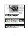
Figure 4.4: One pixel in the resampled image corresponds to a group of pixels in the original image
Although the nearest neighbor downsamping significantly reduces information contained in the
original image by ignoring a big amount of pixels, it preserves sharp edges and the strong
bipolarity of black and white pixels. Because of this, the nearest neighbor downsamping is
suitable in combination with the “edge detection” feature extraction method described in section
4.3.2.
4.2.2
Weighed-average downsampling
In contrast with the nearest-neighbor method, the weighted-average downsamping considers all
pixels from a corresponding group of pixels in the original image.
Let rx and ry be a horizontal and vertical aspect ratio of the resampled image. The value of
the pixel [ x′, y ′] in the destination image is computed as a mean of source pixels in the range
[ xmin , ymin ] to [ xmax , ymax ] :
f ′ ( x′, y ′ ) =
x
( xmax
max
1
− xmin ) ⋅ ( ymax − ymin ) i = xmin
ymax
∑ ∑ f ( i, j )
j = ymin
where:
y′
y′ + 1
x′
x′ + 1
xmin = ; ymin = ; xmax =
; ymax =
ry
ry
rx
rx
30
The weighted-average method of downsampling does not preserve sharp edges of the image (in
contrast with the previous method). You can see the visual comparison of these two methods in
Figure 4.5.
n′
m′
n′
n
m′
m
n
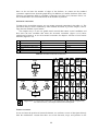
m
Figure 4.5: (a) Nearest-neighbor resampling significantly reduces information contained in
the original image, but it preserves sharp edges. (b) Weighted average resampling gives a
better visual result, but the edges of the result are not sharp.
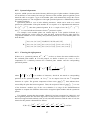
4.3 Feature extraction
Information contained in a bitmap representation of an image is not suitable for processing by
computers. Because of this, there is need to describe a character in another way. The description
of the character should be invariant towards the used font type, or deformations caused by a
skew. In addition, all instances of the same character should have a similar description. A
description of the character is a vector of numeral values, so-called “descriptors”, or “patterns”:
x = ( x0 ,…, xn−1 )
Generally, the description of an image region is based on its internal and external
representation. The internal representation of an image is based on its regional properties, such
as color or texture. The external representation is chosen when the primary focus is on shape
characteristics. The description of normalized characters is based on its external characteristics
because we deal only with properties such as character shape. Then, the vector of descriptors
includes characteristics such as number of lines, bays, lakes, the amount of horizontal, vertical
and diagonal or diagonal edges, and etc. The feature extraction is a process of transformation of
data from a bitmap representation into a form of descriptors, which are more suitable for
computers.
If we associate similar instances of the same character into the classes, then the descriptors
of characters from the same class should be geometrically closed to each other in the vector
space. This is a basic assumption for successfulness of the pattern recognition process.
This section deals with various methods of feature extraction, and explains which method is
the most suitable for a specific type of character bitmap. For example, the “edge detection”
method should not be used in combination with a blurred bitmap.
4.3.1
Pixel matrix
The simplest way to extract descriptors from a bitmap image is to assign a brightness of each
pixel with a corresponding value in the vector of descriptors. Then, the length of such vector is
equal to a square ( w ⋅ h ) of the transformed bitmap:
31
i
xi = f , mod w ( i )
w
where i ∈ 0,… , w ⋅ h − 1 .
Bigger bitmaps produce extremely long vector of descriptors, which is not suitable for
recognition. Because of this, size of such processed bitmap is very limited. In addition, this
method does not consider geometrical closeness of pixels, as well as its neighboring relations.
Two slightly biased instances of the same character in many cases produce very different
description vectors. Even though, this method is suitable if the character bitmaps are too blurry
or too small for edge detection.
h
w
251, 181, 068, 041, 032, 071, 197,
196, 014, 132, 213, 187, 043, 041,
174, 011, 200, 254, 254, 232, 164,
202, 014, 012, 128, 242, 255, 255,
x = 253, 212, 089, 005, 064, 196, 253,
255, 255, 251, 196, 030, 009, 165,
127, 162, 251, 254, 197, 009, 105,
062, 005, 100, 144, 097, 006, 170,
207, 083, 032, 051, 053, 134, 250
Figure 4.6: The “pixel matrix” feature extraction method
4.3.2
Detection of character edges
In contrast with the previous method, the detection of character edges does not consider
absolute positioning of each pixel, but only a number of occurrences of individual edge types in
a specific region of the character bitmap. Because of this, the resulting vector is invariant
towards the intra-regional displacement of the edges, and towards small deformations of
characters.
Bitmap regions
Let the bitmap be described by a discrete function f ( x, y ) , where w and h are dimensions,
such as 0 ≤ x < w and 0 ≤ y < h . We divide it into six equal regions organized to three rows and
two columns in the following way:
(i )
(i )
(i )
(i )
and xmax
be an upper left and bottom right point of a rectangle,
Let xmin
, ymin
, ymax
which determinates the region ri , such as:
•
•
•
•
w
h
(0)
(0)
(0)
(0)
Region r0 : xmin
= 0 , ymin
= 0 , xmax
= − 1 , ymax
= −1
2
3
w
h
(1)
(1)
(1)
(1)
Region r1 : xmin
= , ymin
= 0 , xmax
= w − 1 , ymax
= −1
2
3
h
w
2⋅h
(2)
(2)
(2)
(2)
Region r2 : xmin
= 0 , ymin
= , xmax
= − 1 , ymax
=
−1
3
2
3
w
h
2⋅h
(3)
(3)
(3)
(3)
Region r3 : xmin
= , ymin
= , xmax
= w − 1 , ymax
=
−1
2
3
3
32
2⋅h
w
(4)
(4)
(4)
(4)
Region r4 : xmin
= 0 , ymin
=
, xmax
= , ymax
= h −1
3
2
w
2⋅h
(5)
(5)
(5)
(5)
• Region r5 : xmin
= , ymin
=
, xmax = w − 1 , ymax = h − 1
2
3
There are several ways how to distribute regions in the character bitmap. The regions can be
disjunctive as well as they can overlap each other. The figure 4.7 shows the several possible
layouts of regions.
•
Figure 4.7: Layouts of regions in the character bitmap. The regions can be disjunctive as well as they
can overlap each other.
Edge types in region
Let us define an edge of the character as a 2x2 white-to-black transition in a bitmap. According
to this definition, the bitmap image can contain fourteen different edge types illustrated in figure
4.8.
Figure 4.8: The processed bitmap can contain different types of 2x2 edges.
The statistics of occurrence of each edge type causes uselessly long vector of descriptors.
Because of this, the “similar” types of edges are considered as the same. The following lists
shows how the edges can be grouped together:
1.
2.
3.
4.
5.
6.
7.
8.
0 + 1 (vertical edges)
2 + 3 (horizontal edges)
4 + 6 + 9 (“/”-type diagonal edges)
5 + 7 + 8 (“\”-type diagonal edges)
10 (bottom right corner)
11 (bottom left corner)
12 (top right corner)
13 (top left corner)
For simplicity, assume that edge types are not grouped together. Let η be a number of different
edge types, where hi is a 2x2 matrix that corresponds to the specific type of edge:
1
h0 =
1
0
h7 =
0
0
0 1
1
, h1 =
, h2 =
0
0 1
0
1
0 0
0
, h8 =
, h9 =
0
1 0
0
1
0
, h3 =
0
1
0
0
, h10 =
1
1
33
0
1
, h4 =
1
0
1
1
, h11 =
1
1
0
0
, h5 =
1
1
0
1
, h12 =
1
0
1
1
, h6 =
0
0
1
1
, h13 =
1
1
0
0
1
0
(i )
(i )
(i )
Let ρ be a number of rectangular regions in the character bitmap, where xmin
, ymin
, xmax
and
(i )
ymax
are boundaries of the region ri ( i ∈ 0… ρ − 1 ). If the statistics consider η different edge
types for each of ρ regions, the length of the resulting vector x is computed as η ⋅ ρ :
x = ( x0 , x1 ,… , xη ⋅ρ −1 )
Feature extraction algorithm
At first, we have to embed the character bitmap f ( x, y ) into a bigger bitmap with white
padding to ensure a proper behavior of the feature extraction algorithm. Let the padding be one
pixel wide. Then, dimensions of the embedding bitmap will be w + 2 and h + 2 . The
embedding bitmap f ′ ( x, y ) is then defined as:
if
1
f ′ ( x, y ) =
f ( x − 1, y − 1) if
x = 0 ∨ y = 0 ∨ x = w +1∨ y = h +1
¬ ( x = 0 ∨ y = 0 ∨ x = w + 1 ∨ y = h + 1)
where w and h are dimensions of character bitmap before embedding. Color of the padding is
white (value of 1). The coordinates of pixels are shifted one pixel towards the original position.
The structure of vector of output descriptors is illustrated by the pattern below. The notation
h j @ ri means “number occurrences of an edge represented by the matrix h j in the region ri ”.
(
)
x = h 0 @ r0 , h1 @ r0 ,… , hη −1 @ r0 , h 0 @ r1 , h1 @ r1 ,… , hη −1 @ r1 , h 0 @ rρ −1 , h1 @ rρ −1 ,… , hη −1 @ rρ −1
region r1
region r0
region rρ −1
We compute the position k of the h j @ ri in the vector x as k = i ⋅η + j , where η is the
number of different edge types (and also the number of corresponding matrices).
The following algorithm demonstrates the computation of the vector of descriptors x :
x
for each region ri , where i ∈ 0,… , ρ − 1 do
zeroize vector
begin
for each pixel
[ x, y ]
in region
(i )
(i )
(i )
(i )
ri ,where xmin
≤ x ≤ xmax
and ymin ≤ y ≤ ymax do
begin
for each matrix
begin
if
h j , where j ∈ 0,… ,η − 1 do
f ′ ( x, y )
hj =
f ′ ( x, y + 1)
f ′ ( x + 1, y )
then
f ′ ( x + 1, y + 1)
begin
let
k = i ⋅η + j
let x k = x k + 1
end
end
end
end
34
4.3.3
Skeletonization and structural analysis
The feature extraction techniques discussed in the previous two chapters are based on the
statistical image processing. These methods do not consider structural aspects of analyzed
images. The small difference in bitmaps sometimes means a big difference in the structure of
contained characters. For example, digits ‘6’ and ‘8’ have very similar bitmaps, but there is a
substantial difference in their structures.
The structural analysis is based on higher concepts than the edge detection method. It does
not deal with terms such as “pixels” or “edges”, but it considers more complex structures (like
junctions, line ends or loops). To analyze these structures, we must involve the thinning
algorithm to get a skeleton of the character. This chapter deals with the principle of
skeletonization as well as with the principle of structural analysis of skeletonized image.
The concept of skeletonization
The skeletonization is a reduction of the structural shape into a graph. This reduction is
accomplished by obtaining a skeleton of the region via the skeletonization algorithm. The
skeleton of a shape is mathematically defined as a medial axis transformation. To define the
medial axis transformation and skeletonization algorithm, we must introduce some elementary
prerequisite terms.
ɺɺ be a binary relation between two pixels [ x, y ] and [ x′, y′] , such as aN
ɺɺ b means “ a
Let N
is a neighbor of b ”. This relation is defined as:
[ x, y ] Nɺɺ 8 [ x′, y′] ⇔
[ x, y ] Nɺɺ 4 [ x′, y′] ⇔
x − x′ = 1 ∨ y − y ′ = 1 for eight-pixel neighbourhood
x − x′ = 1 ⊕ y − y ′ = 1 for four-pixel neighbourhood
The border B of character is a set of boundary pixels. The pixel [ x, y ] is a boundary pixel, if it
is black and if it has at least one white neighbor in the eight-pixel neighborhood:
[ x, y ] ∈ B ⇔ f ( x, y ) = 0 ∧ ∃[ x′, y′] : f ( x, y ) = 1 ∧ [ x, y ] Nɺɺ 8 [ x′, y′]
The inner region I of character is a set of black pixels, which are not boundary pixels:
[ x, y ] ∈ I ⇔ f ( x, y ) = 0 ∧ [ x, y ] ∉ B
Figure 4.9: (a) Illustration of the four-pixel and eight-pixel neighborhood. (b) The set of
boundary and inner pixels of character.
The piece Ρ is then a union of all boundary and inner pixels ( Ρ = B ∪ I ). Since there is only
one continuous group of black pixels, all black pixels belong to the piece Ρ . The principle and
the related terminology of the skeletonization are similar to the piece extraction algorithm
discussed in section 3.2.1.
35
Medial axis transformation
The medial axis transformation of the piece Ρ defined as follows. For each inner pixel p ∈ I ,
we find the closest boundary pixel pb ∈ B . If a pixel p has more than one such neighbor, it is
said to belong to the medial axis (or skeleton) of the Ρ . The concept of the closest boundary
pixel depends on the definition of the Euclidean distance between two pixels in the orthogonal
coordinate system. Mathematically, the medial axis (or skeleton) S is a subset of the Ρ defined
as:
p ∈ S ⇔ ∃p1∃p2 : p1 ∈ B ∧ p2 ∈ B ∧ d ( p, p1 ) = d ( p, p2 ) = min {d ( p, p′ )}
p ′∈B
The pixel p belongs to the medial axis S if there exists at least two pixels p1 and p2 , such as
Euclidean distance between pixels p and p1 is equal to the distance between pixels p and p2 ,
and these pixels are closest boundary pixels to pixel p .
The Euclidean distance between two pixels p1 = [ x1 , y1 ] and p2 = [ x2 , y2 ] is defined as:
d ( p1 , p2 ) = 2 ( x1 − x2 ) ⋅ ( x1 − x2 )
2
2
Skeletonization algorithm
Direct implementation of the mathematical definition of the medial axis transformation is
computationally expensive, because it involves calculating the distance from every inner pixel
from the set I to every pixel on the boundary B .
The medial axis transformation is intuitively defined by a so-called “fire front” concept.
Consider that a fire is lit along the border. All fire fronts will advance into the inner of character
at the same speed. The skeleton of a character is then a set of pixels reached by more than one
fire front at the same time.
The skeletonization (or thinning) algorithm is based on the “fire front” concept. The
thinning is a morphological operation, which preserves end-pixels and does not break
connectivity. Assume that pixels of the piece are black (value of zero), and background pixels
are white (value of one).
The thinning is an iterative process of two successive steps applied to boundary pixels of a
piece. With reference to the eight-pixel neighborhood notation in figure 4.9, the first step flags a
boundary pixel p for deletion if each of the following conditions is satisfied:
•
At least one of the top, right and bottom neighbor of the pixel p must be white (the
pixel p is white just when it does not belong to the piece Ρ ).
pt ∉ Ρ ∨ p r ∉ Ρ ∨ pb ∉ Ρ
•
At least one of the left, right and bottom neighbor of pixel p must be white.
pl ∉ Ρ ∨ p r ∉ Ρ ∨ pb ∉ Ρ
•
The pixel p must have at least two, and at most six black neighbors from the piece Ρ .
This condition prevents the algorithm from erasing end-points and from breaking the
connectivity.
36
{
}
ɺɺ p′ ∧ p′ ∉ Ρ ≤ 6
2 ≤ p ′ pN
8
•
The number of white-to-black transitions in the ordered sequence
p t , p tr , p r , p br , p b , p bl , p l , p tl , p t must be equal to one.
(
v( p
) (
∉ Ρ) + v ( p
) (
∈ Ρ ∧ p ∉ Ρ) + v ( p ∈ Ρ ∧ p
) (
∉ Ρ) + v ( p
v p t ∈ Ρ ∧ p tr ∉ Ρ + v ptr ∈ Ρ ∧ p r ∉ Ρ + v p r ∈ Ρ ∧ p br ∉ Ρ + v pbr ∈ Ρ ∧ p b ∉ Ρ
b
∈ Ρ ∧ p bl
0 if
v ( x) =
1 if
bl
l
l
tl
tl
)
)
∈ Ρ ∧ pt ∉ Ρ = 1
x
¬x
The first step flags pixel p for deletion, if its neighborhood meets the conditions above.
However, the pixel is not deleted until all other pixels have been processed. If at least one of the
conditions is not satisfied, the value of pixel p is not changed.
After step one has been applied to all boundary pixels, the flagged pixels are definitely
deleted in the second step. Every iteration of these two steps thins the processed character. This
iterative process is applied until no further pixels are marked for deletion. The result of thinning
algorithm is a skeleton (or medial axis) of the processed character.
•
•
Let the piece Ρ be a set of all black pixels contained in skeletonized character.
Let B be a set of all boundary pixels.
The following pseudo-code demonstrates the thinning algorithm more formally. This algorithm
proceeds the medial axis transformation over a piece Ρ .
do // iterative thinning process
let continue = false
let B = 0/
for each pixel p in piece
Ρ do // create a set of boundary pixels
ɺɺ
if ∃p′ : p′ ∉ Ρ ∧ pN8 p′ then // if the pixel p has at least one white neighbor
insert pixel p into set B // but keep it also in Ρ
for each pixel p in set B do // 1.step of the iteration
begin
// if at least one condition is violated, skip this pixel
(
) then continue
¬ ( p ∉ Ρ ∨ p ∉ Ρ ∨ p ∉ Ρ ) then continue
ɺɺ p′ ∧ p′ ∉ Ρ} ≤ 6 then continue
¬ ( 2 ≤ { p ′ pN
)
¬ pt ∉ Ρ ∨ p r ∉ Ρ ∨ pb ∉ Ρ
if
l
if
if
b
8
if
(
v( p
r
) (
∉ Ρ) + v ( p
) (
∈ Ρ ∧ p ∉ Ρ) + v ( p ∈ Ρ ∧ p
) (
∉ Ρ) + v ( p
v p t ∈ Ρ ∧ p tr ∉ Ρ + v p tr ∈ Ρ ∧ p r ∉ Ρ + v p r ∈ Ρ ∧ p br ∉ Ρ + v p br ∈ Ρ ∧ p b ∉ Ρ
b
∈ Ρ ∧ p bl
bl
l
l
then
begin
continue
end
// all tests passed
flag point p for deletion
let continue = true
37
tl
tl
)
)
∈ Ρ ∧ pt ∉ Ρ ≠ 1
end
for each pixel p in set
if p is flagged then
pull point
B do // 2.step of the iteration
p from piece Ρ
while continue = true
Note: The pixel p belongs to the piece Ρ when it is black: p ∈ Ρ ⇔ f ( p ) = 0
Figure 4.10: (a) The character bitmap before skeletonization. (b) The thinning algorithm
iteratively deletes boundary pixels. Pixels deleted in the first iteration are marked by a
light gray color. Pixels deleted in the second and third iteration are marked by dark gray.
(c) The result of the thinning algorithm is a skeleton (or a medial axis).
Structural analysis of skeletonized character
The structural analysis is a feature extraction method that considers more complex structures
than pixels. The basic idea is that the substantial difference between two compared characters
cannot be evaluated by the statistical analysis. Because of this, the structural analysis extracts
features, which describe not pixels or edges, but the more complex structures, such as junctions,
line ends and loops.
Junction
The junction is a point, which has at least three black neighbors in the eight-pixel neighborhood.
We consider only two types of junctions: the junction of three and four lines. The number of
junctions in the skeletonized piece Ρ is mathematically defined as:
{
}
ɺɺ p′}
= { p ∃ p′ : { p, p′} ⊆ Ρ ∧ pN
ɺɺ p′
n3j = p ∃3 p′ : { p, p′} ⊆ Ρ ∧ pN
8
n3j
4
8
Line end
The line end is a point, which has exactly one neighbor in the eight-pixel neighborhood. The
number of line-ends in a skeletonized piece Ρ is defined as:
{
ɺɺ p
ne = p ∃! p1 : { p, p1} ⊆ Ρ ∧ pN
8 1
}
The following algorithm can be used to detect the number of junctions and number line-ends in
a skeletonized piece Ρ :
38
let
nj = 0
let
ne = 0
for each pixel p in piece
begin
let neighbors = 0
for each pixel
if
Ρ do
p′ in neighborhood
{p , p
t
tr
, p r , p br , p b , p bl , p l , p tl
}
do
p′ ∈ Ρ then
let neighbors = neighbors+1
neighbors = 1 then
let ne = ne +1
else if neighbors ≥ 3 then
let n j = n j +1
if
end
Figure 4.11: (a, b) The junction is a pixel, which as at least three neighbors in eightpixel neighborhood. (c) The line end is a pixel, which has only one neighbor in eightpixel neighborhood (d) The loop is a group of pixels, which encloses the continuous
white space.
Loops
It is not easy to determine the number of loops nl in the skeletonized character. The algorithm
is based on the following principle. At first, we must negate the bitmap of the skeletonized
character. Black pixels will be considered as background and white pixels as foreground. The
number of loops in the image is equal to a number of lakes, which are surrounded by these
loops. Since the lake is a continuous group of white pixels in the positive image, we apply the
piece extraction algorithm on the negative image to determine the number of black pieces. Then,
the number of loops is equal to the number of black pieces minus one, because one piece
represents the background of the original image (negated to the foreground). Another way is to
use a series of morphological erosions.
Figure 4.12: (a) We determine the number of lakes in skeleton by applying the
piece-extraction algorithm on negative image. The negative image (b) contains three
pieces. Since the piece 3 is a background, only two pieces are considered as lakes.
(c)(d) The similar skeletons of the same character can differ in the number of
junctions
39
Since we do not know the number of edges of the skeleton, we cannot use the standard
cyclomatic equation know from the graph theory. In addition, two similar skeletons of the same
character can sometimes differ in a number of junctions (see figure 4.12). Because of this, it is
not recommended to use constraints based on the number of junctions.
Structural constraints
To improve the recognition process, we can assume structural constraints in the table 4.1. The
syntactical analysis can be combined by other methods described in previous chapters, such as
edge detection method or pixel matrix.
The simplest way is to use one global neural network that returns several candidates and
then select the best candidate that meets the structural constraints (figure 4.13.a). More
sophisticated solution is to use the structural constraints for adaptive selection of local neural
networks (figure 4.13.b).
0
1
2
3
4
Line ends
Loops
Junctions
BDO08
PQ69
ACGIJLMNRSUVWZ123457
EFTY
HKX
CEFGHIJKLMNSTUVWXYZ123457
ADOPQR09
B8
CDGIJLMNOSUVWZ012357
EFKPQTXY469
ABHR8
Table 4.1: Structural constraints of characters.
A
C
B
Figure 4.13: (a, b) Structural constraints can be applied before and after the recognition by
the neural network. (c) Example of the skeletonized alphabet.
Feature extraction
In case we know the position of structural elements, we can form a vector of descriptors directly
from this information. Assume that there are several line-ends, loops, and junctions in the
40
image. The position of loop is defined by its centre. To form the vector, we must convert
rectangular coordinates of the element into polar coordinates [ r ,θ ] (see figure 4.14):
2⋅ x − w
2⋅ y − h
y′
r = x′2 + y′2 ; θ = atg ; x′ =
; y′ =
w
h
x′
where x′ and y′ are normalized rectangular coordinates.
The length and the structure of resulting vector vary according to a number and type of
structural elements contained in the character. Since the structural constraints divide characters
into the several classes, there are several possible types of description vector. Each type of
vector corresponds to one class of character.
For example, consider character with two line ends and one junction. This constraint
determines the following class of possible characters: (G, I, J, L, M, N, S, U, V, W, Z, 1, 2, 3, 5,
7). We define a vector of descriptors to distinguish between these characters as follows:
x = ( r1 ,θ1 , r2 ,θ 2 , r3 ,θ3 )
line end line end junction
2
1
−1
w
[ x, y ]
0
1
−1
[ r ,θ ]
r
h
θ
0
1
Figure 4.14: (a) The skeleton of the character contains several structural elements, such
as junctions, loops and line ends. (b, c) Each element can be positioned in the
rectangular or polar coordinate system.
41
Chapter 5
Recognition of characters
The previous chapter deals with various methods of feature extraction. The goal of these
methods is to obtain a vector of descriptors (so-called pattern), which comprehensively
describes the character contained in a processed bitmap. The goal of this chapter is to introduce
pattern recognition techniques, such as neural networks, which are able to classify the patterns
into the appropriate classes.
5.1 General classification problem
The general classification problem is formulated using the mapping between elements in two
sets. Let A be a set of all possible combinations of descriptors, and B be a set of all classes.
The classification means the projection of group of similar element from the set A into a
common class represented by one element in the set B . Thus, one element in the set B
corresponds to one class. Usually the group of distinguishable instances of the same character
corresponds to the one class, but sometimes one class represents two mutually indistinguishable
characters, such as “0” and “O”.
Let F be a hypothetic function that assign each element from the set A to an element from
the set B :
F :A→ B
xˆ = F (x)
where x ∈ A is a description vector (pattern) which describes the structure of classified
character and xˆ ∈ B is a classifier, which represents the semantics of such character .
The function F is the probably best theoretical classificator, but its construction is
impossible since we cannot deal with each combination of descriptors. In praxis, we construct
pattern classifier by using only a limited subset of the A → B mappings. This subset is known
as a “training set”, such as At ⊂ A and Bt ⊂ B . Our goal is to construct an approximation
Fɶ ( x, w ) of the hypothetic function F , where w is a parameter that affects the quality of the
approximation:
Fɶ ( w ) : At → Bt
xˆ = Fɶ ( x, w )
where x ∈ At ⊂ A , xˆ ∈ Bt ⊂ B . Formally we can say that F̂ ( w ) is a restriction of the projection
F over a set At ⊂ A . We assume that for each xi ∈ At we know the desired value xˆ i ∈ Bt :
x 0 → xˆ 0 , x1 → xˆ 1 , x 2 → xˆ 2 ,… , x n −1 → xˆ n −1
42
F
A
Fɶ ( w )
x
B
x̂
At
Bt
Figure 5.1: The projection between sets A and B . The F is a hypothetic function that maps every
possible combination of input pattern x ∈ A to a corresponding class xˆ ∈ B . This projection is
approximated by a function Fɶ ( w ) , which maps input patterns from training set At into the
corresponding classes from the set Bt
The problem is to find an optimal value (or values) of a parameter w . The w is typically a
vector (or matrix) of syntactical weights in a neural network. According to this parameter, the
values of the function Fɶ ( x, w ) should be as closest as possible to the values of F ( x ) for input
patterns x from the training set At . We define an error function to evaluate worthiness of the
parameter w :
E (w) =
1 m −1 ɶ
F ( xi , w ) − xˆ i
2 i =0
∑(
)
2
where m is a number of patterns x 0 … x m −1 in the training set At . Let w + to be an optimal
value of the parameter w , such as w = arg min { E ( w )} . Then, the approximation Fɶ ( x, w ) of
+
w∈W
+
the function F ( x ) is considered as adapted. The adapted approximation Fɶ ( x, w + ) simulates
original function F ( x ) for patterns x from the training set At . In addition, this approximation
is able to predict the output classifier x̂ for unknown pattern x from the “test” set Ax
( Ax = A − At ). The function with such prediction ability partially substitutes the hypothetic
classificator F ( x ) . Since the function Fɶ ( x, w ) is only a model, we use a feed-forward neural
network for its implementation.
5.2 Biological neuron and its mathematical models
For a better understanding of artificial neural network architecture, there is a need to explain the
structure and functionality of a biological neuron. The human brain is a neural network of about
ten billions interconnected neurons. Each neuron is a cell that uses a biochemical reaction to
process and transmit information. The neural cell has a body of size about several micrometers
and thousands of input connections called “dendrites”. It also has one output connection called
“axon”, which can be several meters long. The data flow in the biological neural network is
represented by electrical signal, which propagates along the axon. When the signal reaches a
synaptic connection between the axon and a consecutive dendrite, it relieves molecules of
chemical agent (called mediators or neuro-transmitters) into such dendrite. This action causes a
local change of polarity of a dendrite transmission membrane. The difference in the polarity of
the transmission membrane activates a dendrite-somatic potential wave, which advances in a
system of branched dendrites into the body of neuron.
43
Figure 5.2: The biological neuron
The biological neural network contains two types of synaptic connections. The first is an
excitive connection, which amplifies the passing signal. The second (inhibitive) connection
suppresses the signal. The behavior of the connection is represented by its “weight”. The neural
network contains mechanism which is able to alter the weights of connections. Because of this,
the system of synaptic weights is a realization of human memory. As the weights are
continually altered, the old information is being forgotten little by little.
axon
terminal button of axon
dendrite
neuro-transmitters
Cell body
dendrite
terminal buttons
Figure 5.3: (a) Schematic illustration of the neural cell (b) The synaptic connection
between a dendrite and terminal button of the axon
Since the problematic of the biological neuron is very difficult, the scientists proposed several
mathematical models, such as McCulloch-Pitts binary threshold neuron, or the percepton.
5.2.1
McCulloch-Pitts binary threshold neuron
The McCulloch-Pitts binary threshold neuron was the first model proposed by McCulloch and
Pitts in 1943. The neuron has only two possible output values (0 or 1) and only two types of the
synaptic weights: the fully excitative and the fully inhibitive. The excitative weight (1) does not
affect the input, but the inhibitive one negates it (-1).
44
The weighted inputs are counted together and processed by a neuron as follows:
J −1
y = g wi , j ⋅ x j − ϑi
j =0
0 if ξ < 0
g (ξ ) =
1 if ξ ≥ 0
∑
This type of neuron can perform logical functions such as AND, OR, or NOT. In addition,
McCulloch and Pitts proved that synchronous array of such neurons is able to realize arbitrary
computational function, similarly as a Turing machine. Since the biological neurons have not
binary response (but continuous), this model of neuron is not suitable for its approximation.
5.2.2
Percepton
Another model of neuron is a percepton. It has been proved that McCulloch-Pitts networks with
modified synaptic connections can be trained for the recognition and classification. The training
is based on a modification of a neuron weights, according to the reaction of such neuron as
follows. If the neuron is not active and it should be, we increase the weights. If the neuron is
active and it should not be, we decrease them. This principle was been used in a first model of
the neural classifier called ADALINE (adaptive linear neuron). The major problem of such
networks is that they are not able to solve linearly nonseparable problems.
This problem has been solved when the scientists Rumelhart, Hilton and Williams proposed
the error back-propagation method of learning for multilayered percepton networks. The simple
McCulloch-Pitts binary threshold neurons have been replaced by neurons with continuous
saturation input/output function.
Percepton has multiple analogous inputs and one analogous output. Let xo … x j −1 be inputs
with corresponding weights wi ,0 … wi , j −1 . The weighted inputs are counted, thresholded and
saturated together in the following way:
J −1
y = g wi , j ⋅ x j − ϑi
j =0
1
g (ξ ) =
1 + e −ξ
∑
where g (ξ ) is a sigmoid saturation function (see figure 5.4.b) and ϑi is a threshold value.
Sometimes, the threshold is implemented as a dedicated input with a constant weight of -1 (see
figure 5.4.a). Then, the function of a neuron can be simplified to y = g ( x ⋅ w ) , where x is a
vector of inputs (including the threshold value), and w is a vector of weights (including the
constant weight -1).
45
1
1 + e −ξ
ϑ
x0
x1
x2
∑
g
y
xJ −1
ξ
Figure 5.4: (a) The summation Σ and gain (saturation) g function of the percepton with a
threshold implemented as a dedicated input. (b) The sigmoid saturation function.
5.3 Feed-forward neural network
Formally, the neural network is defined as an oriented graph G = ( N , E ) , where N is a nonempty set of neurons, and E is a set of oriented connections between neurons. The connection
e ( n, n′ ) ∈ E is a binary relation between two neurons n and n′ . The set of all neurons N is
composed of disjunctive sets N 0 , N1 , N 2 , where N i is a set of all neurons from the ith layer.
N = N 0 ∪ N1 ∪ N 2
The jth weight of a ith neuron in a kth layer is denoted as wi(,kj) and the threshold of ith neuron in a
kth layer is denoted as ϑi( k ) . Numbers of neurons for the input (0), hidden (1) and output (2)
layer are denoted as m , n , o , such as m = N 0 , n = N1 and o = N 2 .
The number of neurons in the input layer ( m ) is equal to a length of an input pattern x in
order that each value of the pattern is dedicated to one neuron. Neurons in the input layer do not
perform any computation function, but they only distribute values of an input pattern to neurons
in the hidden layer. Because of this, the input layer neuron has only one input directly mapped
into multiple outputs. Because of this, the threshold value ϑi(0) of the input layer neuron is equal
to zero, and the weights of inputs wi(0)
,0 are equal to one.
The number of neurons in the hidden layer ( n ) is scalable, but it affects the recognition
abilities of a neural network at a whole. Too few neurons in the hidden layer causes that the
neural network would not be able to learn new patterns. Too many neurons cause network to be
overlearned, so it will not be able to generalize unknown patterns as well.
The information in a feed-forward neural network is propagated from lower layers to upper
layers by one-way connections. There are connections only between adjacent layers, thus feedforward neural network does not contain feedback connections, or connections between
arbitrary two layers. In addition, there exist no connections between neurons from the same
layer.
46
y1
y0
Data flow
ϑ0(2)
yo −1
ϑ1(2)
z0
ϑ0(1)
ϑ
(1)
1
ϑo(2)
−1
w(2) i , j
z1
zn −1
ϑ
(1)
n −1
w(1) i , j
ϑ0(0)
ϑm(0)−1
ϑ1(0)
x0
xm −1
x1
Figure 5.5: Architecture of the three layer feed-forward neural network.
5.4 Adaptation mechanism of feed-forward neural network
There has been proven that a multilayered neural network composed of perceptons with a
sigmoid saturation function can solve an arbitrary non-linear problem. Mathematically, for each
function F : ℝ m → ℝ o there exists a multilayered feed-forward neural network that is able to
realize this function. The proof is based on the Kolmogorov’s theorem, which tells that every
continuously growing function f defined on interval 0,1
f ( x0 … xm −1 ) =
m
can be written as:
m −1
2⋅m
∑α ∑φ ( x )
i
i =0
i, j
j =0
j
where α i are properly chosen continuous functions with one parameter.
The problem is how to construct the neural network corresponding to a given non-linear
function. At first, we choose a proper topology of the network. The number of neurons in the
input and output layer is given by lengths of the input and output patterns, while the number of
neurons in the hidden layer is scalable.
An adaptation of the neural network means finding the optimal parameter w + of the
approximation function Fɶ ( x, w ) discussed in section 5.1. Let us define two error functions to
evaluate a worthiness of the parameter w :
Et =
1
2
At
∑ ( Fɶ ( x , w ) − xɶ )
i
i
2
; Ex =
i
1
2
Ax
∑ ( Fɶ ( x , w ) − xɶ )
i
2
i
i
where subscript “t” means “train”, and “x” means “test”. The Et is an error function defined for
patterns from the training set, and E x for patterns from the test set. The response of the neural
network to an input pattern x is given as y = Fɶ ( x , w ) .
i
i
The error function Et goes down as a number of neurons in the hidden layer grows. This
relation is valid also between the function Et and a number of iterative steps of the adaptation
process. These relations can be mathematically described as follows:
47
lim Et = 0 ; lim Et = 0
n →∞
k →∞
where n is the number of neurons in the input layer and k is the number of iteration steps of
the adaptation process.
The error function E x does not have a limit at zero as n and k goes to infinity. Because of
this, there exists an optimal number of neurons and optimal number of iteration steps, in which
the function E x has a minimum (see figure 5.6).
E
Ex
Et
n or k
Figure 5.6: Dependency of error functions Et and E x on the number of neurons in input layer ( n )
and the number of iteration steps ( k ).
For simplicity, we will assume only a feed-forward neural network with one layer of hidden
neurons defined in section 5.3. All neurons in adjacent layers are connected by oriented
connections. There are no feedback connections, or connections between neurons within a
single layer.
The activities of hidden and output neurons are defined as:
m −1
n −1 (2)
(1)
zi = g wi(1)
wi , j ⋅ z j − ϑi(2)
, j ⋅ x j − ϑi ; yi = g
j =0
j =0
∑
∑
activities of neurons in the hidden layer
activities of neurons in the output layer
where g (ξ ) is a sigmoid saturation function (see figure 5.4.b).
5.4.1
Active phase
Evaluation of the activities of hidden and output neurons is performed in so-called “active
phase”. The active phase consists of two steps in three-layer neural networks. The first step is an
evaluation of activities zi in the hidden layer, and the second step is an evaluation of activities
yi . Since the evaluation of activities is performed from bottom layers to top ones, the term
“feed-forward” refers to this principle. The active phase corresponds to an approximation
Fɶ ( x, w ) of function F ( x ) , and it is performed every time when there is a need to classify the
input pattern x .
The following pseudo-code demonstrates the active phase of feed-forward neural network.
The notation is the same as in figure 5.5.
48
w , // vector of thresholds and weights
x ; // input pattern to be classified
output: z , // vector of activities of neurons in hidden layer
y // vector of activities of neurons in output layer (neural
procedure activePhase (input:
network response)
)
begin
// first step: evaluate activities of neurons in the hidden layer
for each neuron in hidden layer with index
begin
let
ξ = w ϑi(1)
for each input with index
let
let
i ∈ 0,… , n − 1 do
j ∈ 0,…, m − 1 do
ξ = ξ + w wi(1)
, j ⋅ xj
zi = g (ξ )
end
// second step: evaluate activities of neurons in the output layer
for each neuron in output layer with index
begin
let
ξ = w ϑi(2)
for each input with index
let
let
i ∈ 0,…, o − 1 do
j ∈ 0,… , n − 1 do
ξ = ξ + w wi(2)
,j ⋅ zj
yi = g (ξ )
end
end
5.4.2
Partial derivatives and gradient of error function
The goal of the training phase is to find optimal values of thresholds and weights to minimize
the error function Et . Adaptation phase is an iterative process in which a response y to an input
pattern x is compared with the desired response x̂ . The difference between the obtained and
desired response is used for a correction of weights. The weights are iteratively altered until the
value of the error function Et is negligible.
Gradient of error function related to a single pattern
We compute a gradient g of an error function related to a single pattern x with desired and
obtained responses y and x̂ . The gradient g is computed in direction from upper layers to
lower layers as follows:
At first, we compute components of the gradient related to thresholds ϑi(2) in the output
layer as
∂E
= ( yi − xˆi ) ⋅ (1 − yi ) ⋅ yi
∂ϑi(2)
49
Then, we compute components of the gradient related to thresholds ϑi(1) in the hidden layer.
∂E
These components are computed using the components
from the previous step as
∂ϑi(2)
follows:
o −1
∂E
∂E (2)
=
z
⋅
1
−
y
⋅
w
i (
i)
(1)
(2) i , j
∂ϑi
j = 0 ∂ϑi
∑
(1)
Similarly, we compute components of the gradient related to weights wi(2)
, j and wi , j in the
following way:
∂E
∂E
∂E
∂E
= (2) ⋅ z j ;
= (1) ⋅ x j
(2)
(1)
∂wi , j ∂ϑi
∂wi , j ∂ϑi
The gradient g is a vector of components is given as follows:
∂E
∂E
∂E
∂E
∂E
∂E
∂E
∂E
g = (1) ,⋯, (1) , (2) ,⋯ , (2) , (1) ,⋯, (1)
, (2) ,⋯, (2)
∂ϑ
w
w
w
w
∂
ϑ
∂
ϑ
∂
ϑ
∂
∂
∂
∂
0
n
−
1
0
o
−
1
0,0
n
−
1,
m
−
1
0,0
o
−
1,
n
−
1
Overall gradient
The overall gradient is defined as a summary of gradients related to individual patterns of the
training set At . Let g x / xˆ be a gradient related to a training pair x / xˆ . The overall gradient is
At
computed as
∑g
x / xˆ
.
x / xˆ
5.4.3
Adaptation phase
The adaptation phase is an iterative process of finding optimal values of weight and thresholds,
for which a value of the error function Et is in a local minimum. The figure 5.7 schematically
illustrates a graph of the function Et - so called “error landscape”. Generally, the error
landscape is w + 1 dimensional, where w is a cardinality of the vector of thresholds and
weights, such as:
(
(1)
(1)
(2)
(2)
w = ϑ0(1) ,⋯,ϑn(1)−1 ,ϑ0(2) ,⋯ ,ϑo(2)
−1 , w0,0 ,⋯ , wn −1, m −1 , w0,0 ,⋯ , wo −1, n −1
50
)
Et
w
Figure 5.7: The numeric approach of finding the global minimum in the error landscape.
The vector of optimal thresholds and weights w + is represented by a global minimum in the
error landscape. Since we cannot compute this minimum analytically, we have to use a numeric
approach. There are various numeric optimization algorithms, such as Newton’s method, or the
gradient descent. We use the gradient descent algorithm to find the global minimum in the error
landscape. The single step of the iterative algorithm can looks like follows:
k +1 ( l )
i
ϑ
k +1
= kϑi(l ) − λ
wi(,l j) = k wi(,l j) − λ
∂E
∂ ϑ
k
(l )
i
(
+ µ ⋅ kϑi(l ) −
∂E
+µ⋅
∂ wi(,l j)
k
(
k
wi(,l j) −
k −1 ( l )
i
ϑ
k −1
)
wi(,l j)
)
where k wi(,l j) is a weight of the connection between the ith neuron in lth layer and jth neuron in l1th layer computed in a kth step of iterative process.
The speed of convergence is represented by a parameter λ . Too small value of the
parameter λ causes excessively slow convergence. Too big value of the λ breaks the
monotony of convergence. The µ is a momentum value, which prevents the algorithm of
getting stuck in local minimums.
∂E
∂E
Note: The notation g (l ) means “the component
of the vector (or gradient). The
∂ϑi(l )
∂ϑi
∂E
is a partial derivative of error function E by the threshold value ϑi(l ) . Similarly, the
∂ϑi(l )
∂E
is a partial derivative of function E by the value of weight wi(,l j) .
∂wi(,l j)
The whole adaptation algorithm of feed-forward neural network can be illustrated by the
following pseudo code.
51
At , // training set of patterns x / xˆ
procedure adaptation (input:
λ,
µ,
// speed of convergence
// momentum value
kmax , // maximum number of iterations
ε
, // precision of adaptation process
w + , // vector of optimal weights and thresholds
output:
)
begin
initialize weights and thresholds in
let
w to random values
w prev = w // we haven’t a previous value of w at the beginning
let
k =0, E =∞
while k ≤ kmax ∧ E > ε do
begin
// compute overall gradient
zeroize overall gradient
for each pair
begin
g
x / xˆ of At do
g x / xˆ for training pair x / xˆ
zeroize gradient g x / xˆ
activePhase( w , x , z , y )// compute activities z , y
// compute gradient
for each threshold
ϑi(2)
do
for each threshold
ϑi(1)
do
∂E
g x / xˆ (1) = zi ⋅ (1 − yi ) ⋅
∂ϑi
∂E
g x / xˆ (2) = ( yi − xˆi ) ⋅ (1 − yi ) ⋅ yi
∂ϑi
o −1
∂E
(2)
(2) ⋅ w wi , j
j =0
∂ϑi
∂E
∂E
do g x / xˆ
= g x / xˆ (2) ⋅ z j
(2)
∂ϑi
∂wi , j
∑g
x / xˆ
for each weight
wi(2)
,j
for each weight
∂E
∂E
wi(1)
=
g
(1) ⋅ x j
ˆ
, j do g x / xˆ
x
/
x
(1)
∂wi , j
∂ϑi
let g = g + g x / xˆ
end
// alter values of thresholds and weights according to the gradient
for each threshold
ϑi(l )
in
g
w + do
(
∂E
w next ϑi(l ) = w ϑi(l ) − λ ⋅ g (l ) + µ ⋅ w ϑi(l ) − w prev ϑi(l )
∂ϑi
(l )
for each weight wi , j in w + do
let
)
∂E
w next wi(,l j) = w wi(,l j) − λ ⋅ g (l ) + µ ⋅ w wi(,l j) − w prev wi(,l j)
∂wi , j
let w prev = w , w = w next
(
let
end
let
w+ = w
end
52
)
5.5 Heuristic analysis of characters
The segmentation algotithm described in chapter three can sometimes detect redundant
elements, which do not correspond to proper characters. The shape of these elements after
normalization is often similar to the shape of characters. Because of this, these elements are not
reliably separable by traditional OCR methods, although they vary in size as well as in contrast,
brightness or hue. Since the feature extraction methods described in chapter four do not consider
these properties, there is a need to use additional heuristic analyses to filter non-character
elements. The analysis expects all elements to have similar properties. Elements with
considerably different properties are treated as invalid and excluded from the recognition
process.
The analysis consists of two phases. The first phase deals with statistics of brighness and
contrast of segmented characters. Characters are then normalized and processed by the piece
extraction algorithm.
Since the piece extraction and normalization of brightness disturbs statistical properties of
segmented characters, it is necessary to proceed the first phase of analysis before the application
of the piece extraction algorithm.
In addition, the heights of detected segments are same for all characters. Because of this,
there is a need to proceed the analysis of dimensions after application of the piece extraction
algorithm. The piece extraction algorithm strips off white padding, which surrounds the
character.
Respecting the constraints above, the sequence of steps can be assembled as follows:
1.
2.
3.
4.
Segment the plate (result is in figure 5.8.a).
Analyse the brightness and contrast of segments and exclude faulty ones.
Apply the piece extraction algorithm on segments (result is in figure 5.8.b).
Analyse the dimensions of segments and exclude faulty ones.
Figure 5.8: Character segments before (a) and after (b) application of the piece extraction
algorithm. This algorithm disturbs statistical properties of brightness and contrast.
If we assume that there are not big differences in brightness and contrast of segments, we can
exclude the segments, which considerably differs from the mean. Let ith segment of plate be
defined by a discrete function f i ( x, y ) , where wi and hi are dimensions of the element. We
define the following statistical properties of an element:
The global brightness of such segment is defined as a mean of brightnesses of individual
pixels:
pb(i ) =
wi
hi
∑∑ f ( x, y )
x = 0 y =0
53
The global contrast of the ith segment is defined as a standard deviation of brightnesses of
individual pixels:
wi
hi
∑∑ ( p
(i )
b
pc(i ) =
x =0 y =0
− f ( x, y )
)
2
wi ⋅ hi
The function f ( x, y ) represents only an intensity of grayscale images, but the additional
heuristic analysis of colors can be involved to improve the recognition process. This analysis
separates character and non-character elements on color basis. If the captured snapshot is
represented by a HSV color model, we can directly compute the global hue and saturation of the
segments as a mean of hue and saturation of individual pixels:
ph(i ) =
wi
hi
∑∑
x = 0 y =0
h ( x, y ) ; ps(i ) =
wi
hi
∑∑ s ( x, y )
x = 0 y =0
where h ( x, y ) and s ( x, y ) is a hue and saturation of the certain pixel in the HSV color model.
If the captured snapshot is represented by a RGB color model, there is need to transform it to
the HSV model first.
To determine the validity of the element, we compute an average value of a chosen property
over all elements. For example, the average brightness is computed as pb =
n −1
∑p
(i )
b
, where n is
i =0
a number of elements. The element i is considered as valid, if its global brightness pb(i ) does
not differ more than 16 % from the average brightness pb . The threshold values of individual
properties have been calibrated as follows:
brightness (BRI)
pb(i ) − pb
< 0.16
pb
Contrast (CON)
pc(i ) − pc
< 0.1
pc
hue (HUE)
ph(i ) − ph
< 0.145
ph
Saturation (SAT)
ps(i ) − ps
< 0.24
ps
Height (HEI)
hi − h
< 0.2
h
width/height ratio
(WHR)
0.1 <
wi
< 0.92
hi
If the segment violates at least one of the constraints above, it is considered as invalid and
excluded from the recognition process. The table 5.1 contains properties of elements from figure
5.8. According to this table, elements 0 and 10 have been refused due to an uncommon
width/height ratio, and elements 1 and 4 due to a small height.
54
i
BRI
CON
HUE
SAT
HEI
WHR
0
1
2
3
4
5
6
7
8
9
10
0.247
0.034
0.002
0.084
0.001
0.117
0.063
0.025
0.019
0.019
0.062
0.038
0.096
0.018
0.012
0.003
0.016
0.016
0.011
0.025
0.048
0.009
0.152
0.181
0.030
0.003
0.021
0.002
0.007
0.025
0.012
0.009
0.041
0.236
0.134
0.038
0.061
0.059
0.063
0.056
0.028
0.034
0.045
0.018
0.189
-0.554
0.040
0.189
-0.777
0.189
0.189
0.114
0.114
0.114
0.189
0.093
0.833
0.642
0.625
1.666
0.625
0.562
0.533
0.600
0.533
0.095
Violated
constraints
BRI,HUE,WHR
HUE,HEI
HEI,WHR
WHR
Table 5.1: Properties of segments in figure 5.8. The meaning of abbreviations is as follows:
BRI=brightness, CON=contrast, HUE=hue, SAT=saturation, HEI=height, WHR=width/height ratio.
55
Chapter 6
Syntactical analysis of
recognized plate
6.1 Principle and algorithms
In some situations when the recognition mechanism fails, there is a possibility to detect a failure
by a syntactical analysis of the recognized plate. If we have country-specific rules for the plate,
we can evaluate the validity of that plate towards these rules. Automatic syntax-based correction
of plate numbers can increase recognition abilities of the whole ANPR system.
For example, if the recognition software is confused between characters „8“ and „B“, the
final decision can be made according to the syntactical pattern. If the pattern allows only digits
for that position, the character „8“ will be used rather than the character „B“.
Another good example is a decision between the digit „0“ and the character „O“. The very
small difference between these characters makes their recognition extremely difficult, in many
cases impossible.
6.1.1
Recognized character and its cost
In most cases, characters are recognized by neural networks. Each neuron in an output layer of a
neural network typically represents one character. Let y = ( y 0 , … , y 9 , y A , … , y Z ) be
a vector of output activities. If there are 36 characters in the alphabet, the vector y will be also
36-dimensional.
Let yi be an ith component of the vector y . Then, yi means how much does the input
character corresponds to the ith character in the alphabet, which is represented by this
component. The recognized character χ is represented by the greatest component of the vector
y:
(
χ = chr max { yi }
0≤ i ≤ z
)
where chr ( yi ) is the character, which is represented by the ith component of vector y .
Let y ( S ) be a vector y descendingly sorted according to the values of components. Then,
the recognized character is represented by the first component of so sorted vector:
(
χ = chr y0( S )
)
When the recognition process fails, the first component of y ( S ) can contain invalid
character, which does not match the syntax pattern. Then, it is necessary to use the next valid
character with a worse cost.
56
6.1.2
Syntactical patterns
In praxis, ANPR systems must deal with many different types of plate numbers. Number plates
are not unified, so each country has own type. Because of this, number plate recognition system
should be able to recognize a type of the number plate, and automatically assign the correct
syntactical pattern to it. The assignation of the right syntactical pattern is a fundamental problem
in syntactical analysis.
Syntactical pattern is a set of rules defining characters, which can be used on a certain
position in a plate number. If the plate number P is a sequence of n alphanumerical characters
(
)
P = p (0) … p ( n −1) , then the syntactical pattern `P is a n -tuple of sets `P = ( `p (0) … `p ( n −1) ) ,
and `p (i ) is a set of all allowed characters for the ith position in a plate.
For example, czech number plates can contain digit on a first position followed by a
character denoting the region, where the plate has been registered and five other digits for
a registration number of a car. Formally, the syntactical pattern `P for czech number plates can
looks like this:
{0,1,2,3, 4,5,6,7,8,9} , {C,B,K,H,L,T,N,E,P,A,S,U,J,Z} ,
`P = {0,1,2,3, 4,5,6,7,8,9} , {0,1, 2,3, 4,5,6,7,8,9} ,{0,1, 2,3, 4,5,6,7,8,9} ,
{0,1,2,3, 4,5,6,7,8,9} , {0,1, 2,3, 4,5,6,7,8,9} ,{0,1, 2,3, 4,5,6,7,8,9}
6.1.3
Choosing the right pattern
If there are n syntactical patterns `P (0) … `P ( n−1) , we have to choose the most suitable one for
the evaluated plate number P . For this purpose, we define a metrics (or a cost) δ for a
computation of a similarity between the evaluated plate number and the corresponding
syntactical pattern:
{
δ (`P) = p
where
{p
(i )
p ( i ) ∉ `p ( i )
}
(i )
p ∉ `p
(i )
(i )
}
1
−2
+∑
× 10 ,
(i )
i = 0 max y j
0≤ j ≤ z
n −1
{ }
is a number of characters, which do not match to corresponding
positions in the syntactical pattern `P . Let y (i ) be an output vector for the ith-recognized
{ }
character in a plate. The greatest component of that vector max y (ji )
0≤ j ≤ z
then indicates how
{ } is a cost
successfully the plate has been recognized. Then, the reciprocal value of max y (ji )
0≤ j ≤ z
of the character. Another way of the cost evaluation is a usage of the Smith-Waterman
algorithm to compute the difference between the recognized plate number and the syntactical
pattern.
For example, assume that plate number ‘0B01234’ has been recognized as ‘0801234’, and
the recognition pattern does not allow digit at the second position of a plate. If the character “8”
has been recognized with similarity ratio of 0.90, and other characters with the ratio of 0.95, the
metrics for this pattern is determined as follows.
10−2
δ (`P ) = (1) +
0.95
+
10−2 10−2 10−2 10−2 10−2 10−2
+
+
+
+
+
= 1,07426
0.90 0.95 0.95 0.95 0.95 0.95
57
If there is a pattern that exactly matches to the evaluated plate number, we can say that number
has been correctly recognized, and no further corrections are needed. In addition, it is not
possible to detect a faulty number plate, if it does not break rules of a syntactical pattern.
Otherwise, it is necessary to correct detected plate using the pattern with lowest cost δ :
{ ( )}
( sel )
= arg min δ `P ( i )
`P
0≤ i < n
The correction of a plate means the replacement of each invalid character by another one. If the
character p (i ) at the ith position of the plate P does not match the selected pattern `P ( sel ) , it will
be replaced by the first valid one from y ( s ) . y ( s ) is a sorted vector of output activities denoting
how much the recognized character is similar to an individual character from the alphabet.
Heuristic analysis of a segmented plate can sometimes incorrectly evaluate non-character
elements as characters. Acceptance of the non-character elements causes that the recognized
plate will contain redundant characters. Redundant characters occur usually on sides of the
plate, but rarely in the middle.
If the recognized plate number is longer than the longest syntax pattern, we can select the
nearest pattern, and drop the redundant characters according to it.
58
Chapter 7
Tests and final
considerations
7.1 Choosing the representative set of snapshots
I have captured many of static snapshots of vehicles for the test purposes. Random moving and
standing vehicles with Slovak and Czech number plates have been included. At first, my
objective was to find a representative set of number plates, which are recognizable by humans.
Of course, the set like this contains extremely wide spectrum of plates, such as clear and easy
recognizable as well as plates degraded by the significant motion blur or skew.
Then, a recognition ability of a machine is represented by a ratio between the number of
plates, which have been recognized by the machine, and the number of plates recognized by a
human. Practically, it is impossible to build a machine with the same recognition abilities as a
human has. Because of this, the test like this is extremely difficult and useless.
In praxis, it is more useful to find a representative set of number plates, which can be
captured by an ANPR camera. The position of the camera has a significantly affects the quality
of captured images, and a successfulness of the whole recognition process. The suitable position
of the camera towards the lane can lead to a better set of all possible snapshots. In some
situations, we can avoid of getting skewed snapshots by a suitable positioning of the camera.
Sometimes, this is cleverer than a development of the robust de-skewing mechanisms.
Let S be a representative set of all snapshots, which can be captured by a concrete instance
of the ANPR camera. Some of the snapshots in this set can be blurred, some of them can be too
small, too big, too skewed or too deformed. Because of this, I have divided the whole set into a
following subsets:
S = Sc ∪ Sb ∪ S s ∪ Se ∪ Sl
where S c is a subset of “clear” plates, S b is a subset of blurred plates, S s is a subset of skewed
plates, S e is a subset of plates, which has a difficult surrounding environment, and S l is a
subset of plates with little characters.
59
A
B
C
D
Figure 7.1: Typical snapshot from the set of (a) clear plates (b) plates with little, or blurred
characters (c) skewed plates (d) plates with difficult surrounding environment
7.2 Evaluation of a plate number correctness
Plate numbers recognized by a machine can sometimes differ from the correct ones. Because of
this, there is a need to define formulas and rules, which will be used to evaluate a degree of
plate correctness.
{
Let P be a plate number, and S = P (0) ,… , P ( n-1)
}
be a set of all tested plate numbers.
Then, recognition rate R ( S ) of the ANPR system tested on set S is calculated as:
R(S ) =
1
n
n −1
∑ s (P ) ,
(i )
i =0
where n is a cardinality of the set S , and s (P ) is a correctness score of the plate P . The
correctness score is a value, which express how successfully the plate has been recognized.
Now the question is how to define the correctness score of individual plates. There are two
different approaches, how to evaluate it. The first is a binary score, and the second is a weighted
score.
7.2.1
Binary score
Let us say, that plate number P
(
P = p ,… , p
(0)
( n −1)
) . If
P
(r )
is a sequence of n
alphanumerical characters
is the plate number recognized by a machine, and P ( c ) is the
correct one, then binary score sb of plate P ( r ) is evaluated as follows:
60
( )
sb P
(r )
0 if
=
1 if
P ( r ) ≠ P (c )
P(r ) = P(c)
Two plate numbers are equal, if all characters on corresponding positions are equal:
(P
(r )
) (
)
= P ( c ) ⇔ ∀i∀j : pi( r ) ≠ p (jr ) ⇒ i ≠ j ,
where pi( r ) is the ith character of plate number P ( r )
7.2.2
Weighted score
If P ( r ) is a plate number recognized by a machine, and P ( c ) is the correct one, then weighted
score s w of plate P ( r ) is given as:
sw ( P ( r ) )
{p
=
(r )
i
pi( r ) = pi( c )
{p }
(r )
i
} =m
n
where m is the number of correctly recognized characters, and n is the number of all characters
in plate.
For example if the plate “KE123AB” has been recognized as “KE128AB”, the weighted
correctness score for this plate is 0.85, but the binary score is 0.
7.3 Results
The table 7.1 shows recognition rates, which has been achieved while testing on various set of
number plates. According to the results, this system gives good responses only to clear plates,
because skewed plates and plates with difficult surrounding environment causes significant
degradation of recognition abilities.
Clear plates
Blurred plates
Skewed plates
Average plates
Total number
of plates
68
52
40
177
Total number
of characters
470
352
279
1254
Weighted score
87.2
46.87
51.64
73.02
Table 7.1: Recognition rates of the ANPR system.
61
Summary
The objective of this thesis was to study and resolve algorithmic and mathematical aspects of
the automatic number plate recognition systems, such as problematic of machine vision, pattern
recognition, OCR and neural networks. The problematic has been divided into several chapters,
according to a logical sequence of the individual recognition steps. Even though there is a
strong succession of algorithms applied during the recognition process, chapters can be studied
independently.
This work also contains demonstration ANPR software, which comparatively demonstrates
all described algorithms. I had more choices of programming environment to choose from.
Mathematical principles and algorithms should not be studied and developed in a compiled
programming language. I have considered usage of the Matlab™ and the Java™. Finally, I
implemented ANPR in Java rather than in Matlab, because Java™ is a compromise
programming environment between the Matlab™ and compiled programming language, such as
C++. Otherwise, I would have to develop algorithms in Matlab, and then rewrite them into a
compiled language as a final platform for their usage in the real environment.
ANPR solution has been tested on static snapshots of vehicles, which has been divided into
several sets according to difficultness. Sets of blurry and skewed snapshots give worse
recognition rates than a set of snapshots, which has been captured clearly. The objective of the
tests was not to find a one hundred percent recognizable set of snapshots, but to test the
invariance of the algorithms on random snapshots systematically classified to the sets according
to their properties.
62
Appendix A: Case study
134.jpg
width:488 px
height:366 px
The plate has been
successfully recognized
- no further comment
needed.
Detected band
width: 488 px
height: 30 px
Detected plate
Skew detection
1.44°
Segmentation
Number of detected characters: 10
Recognized plate
RK959AF
63
149.jpg
width:526 px
height:350 px
The plate has been
successfully recognized
- no further comment
needed.
Detected band
width: 526 px
height: 28 px
Detected plate
Skew detection
0.0°
Segmentation
Number of detected characters: 10
Recognized plate
RK959AD
64
034.jpg
width:547 px
height:410 px
The plate has been
successfully recognized
- no further comment
needed.
Detected band
width: 547 px
height: 42 px
Detected plate
Skew detection
-2.656°
Segmentation
Number of detected characters: 11
Recognized plate
LM010BE
65
049.jpg
width:410 px
height:360 px
The plate has been
successfully recognized
- no further comment
needed.
Detected band
width: 410 px
height: 27 px
Detected plate
Skew detection
-5.762°
Segmentation
Number of detected characters: 10
Recognized plate
RK878AC
66
040.jpg
width:576 px
height:432 px
The plate has been
successfully recognized
- no further comment
needed.
Detected band
width: 576 px
height: 21 px
Detected plate
Skew detection
0.0°
Segmentation
Number of detected characters: 11
Recognized plate
BA738DE
67
098.jpg
width: 425 px
height: 330
px
The plate has been
successfully recognized
- no further comment
needed.
Detected band
width: 425 px
height: 28 px
Detected plate
Skew detection
0.0°
Segmentation
Number of detected characters: 9
Recognized plate
1B19839
68
60.jpg
width:424 px
Detected band
width: 424 px
height:336 px
Class: blurred characters
A significant blur
caused improper
detection of the band in
a graph of vertical
projection. In addition,
further heuristic
analyses did not detect
this fault. Because of
this, the incorrect
candidate to number
plate has been
deskewed and then
segmented even though
it does not have any
semantics.
height: 141 px
Detected plate
Point of failure: vertical
projection and heuristic
analysis of band.
Skew detection
0.136°
Segmentation
Number of detected characters: 6
Recognized plate
N/A
69
023.jpg
width:354 px
Detected band
width: 354 px
Detected plate
height:308 px
Class: difficult environment
This is a typical
snapshot with a
difficult surrounding
environment. The table
in the background
contains more
characters in one line
than a number plate in
the foreground. This
fact causes a bigger
amount of horizontal
edges in an area of the
table. The three
detected peaks in the
graph of the horizontal
projection correspond
height: 19 px
to three rows in the
table. Although the
number plate candidate
is wrong, the further
analysis did not refuse
it, because the number
of characters (10) is
within the allowed
range.
Skew detection
-1.169°
Segmentation
Number of detected characters: 10
Recognized plate
0CNCKEP
70
044.jpg
width:530 px
height:397 px
Class: skewed plates
The part of graph
corresponding to the
peak “2” (in vertical
graph) has a wider
distribution due to the
improper vertical
projection caused by a
skew of the plate.
Because of this, the
bottom of the last
character “E” has been
cut off improperly.
Point of failure :
vertical projection –
band clipping
Detected band
width: 530 px
height: 30 px
Detected plate
Skew detection
5.599°
Segmentation
Number of detected characters: 7
Recognized plate
RK892AF
71
067.jpg
width:402 px
Detected band
width: 402 px
height:298 px
Class: extremely small characters
This snapshot contains
extremely small
characters, which are
not distinguishable by a
machine. The number
plate has been properly
detected and characters
have been segmented as
well, but it is very hard
to distinguish between
the “B” and “8” on the
first position and
between the “6” and
“8” on the third
position of plate.
height: 21 px
Detected plate
Point of failure :
character recognition
Skew detection
4.00°
Segmentation
Number of detected characters: 10
Recognized plate
8Y849A4
72
Appendix B: Demo recognition software - User’s manual
JavaANPR is an ANPR recognition software that demonstrates principles described in this
thesis. It is written in the Java programming language. If you want to run it, you will need the
Java 1.5.0 SE runtime environment (or higher).
After downloading the distribution package, please unpack it into a chosen directory. The
distribution package contains compiled program classes, jar archive, source codes and
additional program resources such as bitmaps, neural networks etc.
build
dist
lib
nbproject
resources
src
Compiled classes
Distribution directory, contains JAR file and additional resources
Compile-time libraries
Project metadata and build configuration
Resources, configuration file, bitmaps, neural networks
Source files
1. Cleaning, compiling and building the project (optional)
Normally, you do not have to compile the project, because distribution package already contains
precompiled binaries. If you want to recompile it again, you can do it using the “Apache Ant”
utility.
At first, change a working directory to the “javaanpr”, and type the following command to
clean the previous build of the JavaANPR. Issuing this command will delete whole content of
the build and dist directories:
javaanpr # ant clean
Then, issue the “ant compile” and “ant jar” commands. The “compile” target will
compile all source files in the src directory. The “jar” target will create the “dist” directory
with a jar archive and additional run-time resources.
javaanpr # ant compile
javaanpr # ant jar
2. Running the viewer
You can run the interactive ANPR viewer using the ant by typing the following command:
javaanpr # ant run
If you do not have installed the ANT utility, you can run viewer manually by the following
commands:
javaanpr # cd ./dist
dist # java –jar javaanpr.jar
Another way to run the viewer is a double-click to a javaanpr.jar archive (in the MS
Explorer)
73
Figure B.1: Graphical user interface of the JavaANPR viewer
Important: By default, the program expects the configuration file “config.xml” and other
resources in the working directory. Because of this, please do not run the jar archive from other
directories. Otherwise, the program will not be able to start.
3. Using command-line arguments
Besides the graphical user interface, program also contains additional functions, which are
accessible using the command-line arguments. For more information about it, please run the jar
file with a “-help” command:
Automatic number plate recognition system
Copyright (c) Ondrej Martinsky, 2006-2007
Licensed under the Educational Community License
Usage : java -jar javaanpr.jar [-options]
Where options include:
-help
Displays this help
-gui
Run GUI viewer (default choice)
-recognize -i <snapshot>
Recognize single snapshot
-recognize -i <snapshot> -o <dstdir>
Recognize single snapshot and save report html into
specified directory
-newconfig -o <file>
Generate default configuration file
-newnetwork -o <file>
Train neural network according to specified feature
extraction method and learning parameters (in config.
file) and saves it into output file
-newalphabet -i <srcdir> -o <dstdir>
Normalize all images in <srcdir> and save it to <dstdir>.
3.1
Command-line recognition
If you do not want to use the GUI viewer, you can recognize snapshot by issuing the following
command. The recognized plate will be written to standard output.
74
dist # java –jar javaanpr.jar –recognize –i <name of image>
3.2
Recognition report
Sometimes, it is good to see inside the recognition process of concrete image. Because of this,
JavaANPR supports a generation of HTML reports. The recognition report contains images and
verbose debugging information about each step of the recognition process. HTML report can be
used to determine a point, in which the recognition process failed.
The following command will recognize the image specified by its name, and save the report
into a specified destination directory:
dist # java –jar javaanpr.jar –recognize –i <name of image>
-o <destination directory>
3.3
Creating the default configuration file
Configuration file contains settings and parameters, which are needed during the recognition
process. If configuration file does not exist, program will not be able to start. Because of this,
JavaANPR is able to generate a default configuration file with recommended configuration
settings by the following command:
dist # java –jar javaanpr.jar -newconfig -o <file>
75
Bibliography
[1] Fajmon B.: Numeric Math and Probability, scripts, Faculty of Electrical Engineering
and Communication, Brno, Czech Republic, 2005
[2] Fraser N.: Introduction to Neural Networks,
http://www.virtualventures.ca/~neil/neural/neuron.html
[3] Fukunaga K.: Introduction to statistical pattern recognition, Academic Press, San
Diego, USA, 1990
[4] Gonzalez R., Woods R.: Digital Image Processing, Prentice Hall, Upper Saddle River,
New Jersey, 2002
[5] Kovar M.: Discreet Math, scripts, Faculty of Electrical Engineering
and Communication, Brno, Czech Republic, 2003
[6] Kuba M.: Neural Networks, scripts, Faculty of Informatics, Masaryk University, Brno,
Czech Republic
[7] Kvasnicka V., Benuskova L., Pospichal J., Farkas I., Tino P., Kral A.: Introduction to
Neural Networks, Technical University, Kosice, Slovak Republic
[8] Minsky M., Papert S.: Perceptons. An Introduction to Computational Geometry, MIT
Press:. Cambridge, Massachusetts, 1969
[9] Shapiro V., Dimov D., Bonchev S., Velichkov V., Gluhchev G.: Adaptive License Plate
Image Extraction, International Conference Computer Systems and Technologies,
Rousse, Bulgaria, 2004
[10] Smagt P.: Comparative study of neural network algorithms applied to optical
character recognition, International conference on Industrial and engineering
applications of artificial intelligence and expert systems, Charleston, South Carolina,
USA, 1990
[11] Srivastava R: Transformations and distortions tolerant recognition of numerals using
neural networks, ACM Annual Computer Science Conference, San Antonio, Texas,
USA, 1991
[12] Wang J., Jean J.: Segmentation of merged characters by neural networks and
shortest-path, Symposium on Applied Computing, Indianapolis, Indiana, USA, 1993
[13] Zboril F.: Neural Networks, Department of Intelligent Systems, Faculty of Information
Technology, BUT Brno, Czech Republic
[14] Zhang Y., Zhang C.: New Algorithm for Character Segmentation of License Plate,
Intelligent Vehicles Symposium, IEEE, 2003
[15] ANPR-tutorial.com, Quercus technologies, 2006
76