Download AxoGraph X Data Acquisition Manual

AxoGraph X
Data Acquisition Manual
PLEASE NOTE:
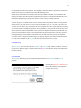
• For the best figure quality when reading this document onscreen, the zoom setting should be 147 %.
• If the zoom setting has changed, type 147 % into the zoom field
• Search for a key-word by clicking on the binoculars icon
in the toolbar at bottom left.
in the toolbar at top right.
• Navigate this document using the bookmarks at left. The bookmarks can be toggled in and out by clicking
the toolbar icon
at bottom left.
• Alternatively navigate using the table of contents on following pages. Clicking on an item of interest will
jump to the relevant page of the main text.
Copyright
Copyright © 1991-2003 by Dr. John Clements All rights reserved.
Disclaimer
All product names mentioned in the AxoGraph 4.9 Data Acquisition Manual are registered trademarks of their
respective manufacturers. Any mention of specific products should not be construed as an endorsement by Axon
Instruments.
ii
Chapters
1
2
3
4
5
6
7
8
9
10
11
12
Introduction
Configuration
Digital Oscilloscope
Digital Chart and Tape Recorder
Electrophysiology Test Pulse
Protocol Driven Acquisition
Create or Edit a Protocol
Online Analysis
The Protocol Launch List
Example Protocols
Precise Acquisition Timing
Optimizing Performance
Contents
1 Introduction........................................................................................................................................................ 1
1.1 Explore the Acquisition Software Without a Digitizer......................................................................... 1
1.2 Hardware Requirements for Data Acquisition........................................................................................ 1
1.3 Install Acquisition Hardware and Software ............................................................................................ 2
1.4 Trouble-Shoot Hardware and Software Installation ............................................................................... 5
1.5 Optionally Remove the Electrophysiology Features .............................................................................. 7
1.6 Summary of Features ............................................................................................................................... 7
2 Configuration ..................................................................................................................................................... 9
2.1 Introduction .............................................................................................................................................. 9
2.2 Connections .............................................................................................................................................. 9
2.3 Channel Names....................................................................................................................................... 10
2.4 Signal Gains............................................................................................................................................ 11
2.5 Holding Levels ....................................................................................................................................... 12
2.6 Save and Load Configuration ................................................................................................................ 13
2.7 Telegraphs .............................................................................................................................................. 13
2.8 Clamp Mode ........................................................................................................................................... 16
3 Digital Oscilloscope ......................................................................................................................................... 18
3.1 Introduction ............................................................................................................................................ 18
3.2 Run Scope............................................................................................................................................... 18
3.3 Hot Keys ................................................................................................................................................. 19
3.4 Display.................................................................................................................................................... 19
3.5 Average................................................................................................................................................... 20
3.6 Timebase................................................................................................................................................. 20
3.7 Trigger .................................................................................................................................................... 21
3.8 Channels ................................................................................................................................................. 23
3.9 Gains ....................................................................................................................................................... 24
3.10 Test Pulse.............................................................................................................................................. 24
3.11 Analyse ................................................................................................................................................. 25
3.12 Custom Analysis .................................................................................................................................. 26
iii
4 Digital Chart and Tape Recorder.................................................................................................................. 28
4.1 Introduction ............................................................................................................................................ 28
4.2 Run Chart................................................................................................................................................ 29
4.3 New Chart............................................................................................................................................... 29
4.4 Hot Keys ................................................................................................................................................. 29
4.5 Event Markers ........................................................................................................................................ 29
4.6 Timebase................................................................................................................................................. 30
4.7 Channels ................................................................................................................................................. 30
4.8 Gains ....................................................................................................................................................... 31
4.9 Test Pulse................................................................................................................................................ 31
4.10 Analyse ................................................................................................................................................. 32
4.11 Custom Analysis .................................................................................................................................. 33
5 Electrophysiology Test Pulse.......................................................................................................................... 34
5.1 Introduction ............................................................................................................................................ 34
5.2 Test Channels ......................................................................................................................................... 35
5.3 Test Pulse Hot Keys ............................................................................................................................... 35
5.4 Test Seal ................................................................................................................................................. 36
5.5 Test Cell.................................................................................................................................................. 36
5.6 Test To Log ............................................................................................................................................ 37
5.7 Test Setup ............................................................................................................................................... 37
5.8 Test Pulse................................................................................................................................................ 38
5.9 Test Link................................................................................................................................................. 38
6 Protocol Driven Acquisition ........................................................................................................................... 39
6.1 Introduction ............................................................................................................................................ 39
6.2 Preview ................................................................................................................................................... 40
6.3 Record..................................................................................................................................................... 40
6.4 Resume ................................................................................................................................................... 41
6.5 Hot Keys ................................................................................................................................................. 41
6.6 Protocol................................................................................................................................................... 42
6.7 File Name ............................................................................................................................................... 42
6.8 Deleting Data Files................................................................................................................................. 43
7 Create or Edit a Protocol................................................................................................................................ 44
7.1 Introduction ............................................................................................................................................ 44
7.2 Create...................................................................................................................................................... 45
7.3 Timebase................................................................................................................................................. 45
7.4 Channels ................................................................................................................................................. 46
7.5 Repetitions.............................................................................................................................................. 47
7.6 Add Pulse................................................................................................................................................ 48
7.7 Define Pulse or Ramp Shape ................................................................................................................. 50
7.8 Define Pulse Train Shape....................................................................................................................... 51
7.9 Edit Pulse................................................................................................................................................ 53
7.10 Delete Pulse.......................................................................................................................................... 53
7.11 Display.................................................................................................................................................. 54
7.12 Trigger .................................................................................................................................................. 56
7.13 Custom Waveform ............................................................................................................................... 57
7.14 Add a Link............................................................................................................................................ 58
7.15 P/N Leak Subtraction ........................................................................................................................... 59
7.16 Extract Protocol.................................................................................................................................... 60
7.17 Convert To Protocol............................................................................................................................. 60
iv
8 Online Analysis ................................................................................................................................................ 61
8.1 Introduction ............................................................................................................................................ 61
8.2 Add Analysis Programs to a Protocol ................................................................................................... 62
8.3 Standard Analysis Programs.................................................................................................................. 63
8.4 Writing New Analysis Programs........................................................................................................... 65
9 The Protocol Launch List ............................................................................................................................... 69
9.1 Introduction ............................................................................................................................................ 69
9.2 Edit Launch List ..................................................................................................................................... 69
9.3 Default Launch Mode ............................................................................................................................ 70
9.4 Open Listed Protocols............................................................................................................................ 71
9.5 Remove the Launch List Features ......................................................................................................... 71
10 Example Protocols ......................................................................................................................................... 72
10.1 Introduction .......................................................................................................................................... 72
10.2 Brief Overview of Each Protocol ........................................................................................................ 72
10.3 Detailed Description of Each Protocol................................................................................................ 74
11 Precise Acquisition Timing........................................................................................................................... 83
11.1 Stability and Accuracy of Regular Trigger ......................................................................................... 83
11.2 Hardware Limitations on the Sampling Rate ...................................................................................... 83
11.3 Timing of Input and Output Events..................................................................................................... 85
12 Optimizing Performance .............................................................................................................................. 87
12.1 Memory and Network Settings............................................................................................................ 87
12.2 Interleave Acquisition and Display ..................................................................................................... 87
12.3 Buffer Acquired Data to Memory ....................................................................................................... 88
12.4 Disable Acquisition Monitor ............................................................................................................... 88
1 Introduction
1.1
1.2
1.3
1.4
1.5
1.6
Explore the Acquisition Software Without a Digitizer
Hardware Requirements for Data Acquisition
Install Acquisition Hardware and Software
Trouble-Shoot Hardware and Software Installation
Optionally Remove the Electrophysiology Features
Summary of Features
1.1 Explore the Acquisition Software Without a Digitizer
The AxoGraph data acquisition package can run in demo mode and generate simulated electrical signals.
This permits the various acquisition programs and options to be explored.
The installer named ‘Install AxoGraph 4.9 Demo’ installs and preloads the acquisition software package.
The acquisition programs can only run in demo mode.
The installer named ‘Install AxoGraph 4.9’ does not preload the acquisition software package. It needs to be
loaded manually, as follows…
Open the AxoGraph 4.9 folder, then the Data Acquisition Package folder.
Move the Acquisition Programs Demo folder into the Plug-In Programs folder.
Launch the AxoGraph 4.9 application.
The installer named ‘Install AxoGraph 4.9 + Acq’ installs and preloads a fully functional acquisition
software package. If no digitizer is connected, the acquisition programs revert to demo mode.
Skip to section 2.2 for more detailed information on the acquisition programs.
1.2 Hardware Requirements for Data Acquisition
Data is acquired to memory, so a minimum of 32 MByte RAM is recommended for episodic data
acquisition, and 64 MByte for continuous acquisition at a high sampling rate (see Section 4.1 for additional
information on memory requirements).
AxoGraph runs on all Power Macintosh computers, and on older Macs with a 680x0 CPU and an FPU. Data
acquisition requires a Digidata 1320 series, or an Instrutech ITC-16 or ITC-18 digitizer. The Digidata 1320
consists of an external unit that connects to the Mac via a SCSI cable. Newer PowerMacs that do not have a
built-in SCSI bus (G4 and newer) will also require the installation of a SCSI card into a PCI bus slot inside
the computer. The Digidata ships with a SCSI card. The ITC-16 and ITC-18 digitizers consist of an external
rack-mounting data acquisition unit and a bus interface card which plugs into a slot inside the computer. For
the ITC-16, interface cards are available for both NuBus and PCI bus computers. The ITC-18 is only
available with a PCI bus card. For more information on digitizer hardware, visit….
Digidata 1320
ITC-16 and ITC-18
http://www.axon.com/CN_Digidata1320.html
http://www.instrutech.com/
2
Summary of hardware requirements
Machine
68K Mac
PowerMac prior to G4*
Power Mac G4 and newer
Digitizer
ITC-16
ITC-16, ITC-18
Digidata 1320 series
ITC-16, ITC-18
Digidata 1320 series
Interface Card
NuBus
PCI Bus
not required – uses built-in SCSI
PCI Bus
SCSI card (shipped with Digidata)
* Very early PowerMacs prior to the 7100 model had a NuBus, not a PCI bus. Check the bus type of any
PowerMac 6000 or 7000 series computer before purchasing an Instrutech digitizer interface card.
Memory Recommendations
32 MB RAM or more for episodic acquisition
64 MB RAM or more for continuous acquisition
Virtual memory is not recommended when running data acquisition package
1.3 Install Acquisition Hardware and Software
This section describes five steps required to set up a computer for data acquisition…
(1) Connect a digitizer to the computer
(2) Load the data acquisition software
(3) Test the software installation
(4) Connect electronic equipment to the digitizer
(5) Describe the connections
(1) Connect a digitizer to the computer
Always shut down the computer before connecting a digitizer.
To connect an Instrutech ITC-16 or ITC-18 digitizer:
An interface card and connecting cable are supplied with the Instrutech digitizer
Open the computer case and install the interface card into an internal slot
(usually a PCI bus slot, but could be a NuBus slot in an old 680x0 Mac)
Close the case and connect the cable between the interface card and the digitizer
Plug in and switch on the digitizer
Power up the computer
To connect an Axon Digidata 1320 series digitizer:
An ‘AdvanSys’ PCI to SCSI card and a SCSI cable are supplied with the Digidata
Open the computer case and install the SCSI card into an internal PCI slot
Close the case and connect the supplied SCSI cable from the card to the Digidata
Plug in and switch on the Digidata
Power up the computer
Insert the AdvanSys CD, and run the installation software
Alternative connection strategy for Axon Digidata 1320 series digitizer
All Mac models prior to the G4 have a built-in SCSI port at the rear of the computer. It is possible to
connect a Digidata 1320 directly to this port, or to daisy-chain it with an external hard drive. However,
the cable supplied with the Digidata will not connect to the Mac’s built-in port, because it uses a
3
different physical format. Cables and adapters for connecting between the three main SCSI port formats
are available at computer shops.
(2) Load the data acquisition software
There are two different installers for AxoGraph 4.9.
• ‘Install AxoGraph 4.9 + Acq’ installs a fully functional acquisition package and preloads the package. The
acquisition programs are automatically loaded into toolbars and the Program menu.
If an item named Acquisition appears under the Program menu, then the acquisition package is preloaded.
The acquisition programs can be run by clicking toolbar buttons at the bottom of the screen, or from
submenus of the Program menu.
• ‘Install AxoGraph 4.9’ installs only a demo version of the acquisition software and does not preload the
acquisition package. The acquisition package will need to be loaded manually, as described below.
If the acquisition package is not preloaded, it can be manually loaded as follows.
Open the AxoGraph 4.9 folder, then the Data Acquisition Package folder.
Move the Acquisition Programs Demo folder into the Plug-In Programs folder.
Launch the AxoGraph 4.9 application.
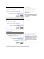
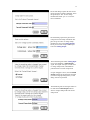
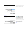
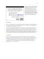
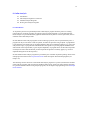
(3) Test the software installation
This section assumes that the AxoGraph data acquisition software has just been loaded for the first time.
If a digitizer has not been installed, skip to step (c).
(a) Make sure the digitizer is plugged in and the power is on.
(b) Connect a cable from Analog Input 0 to Analog Output 0.
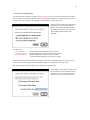
(c) Launch AxoGraph. A toolbar will appear at the bottom of the screen.
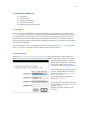
(d) Change the toolbar popup menu setting to Scope.
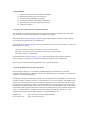
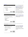
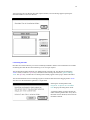
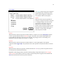
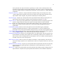
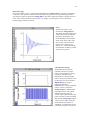
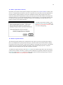
(e) Click on the Run Scope button in the toolbar.
A Scope Window will appear with a
live, updating trace containing a square
pulse.
If AxoGraph can not communicate with
the digitizer, or if initialization of the
digitizer hardware fails, an alert will
appear asking you to check that a
digitizer is connected to the computer,
and that it is switched on. When the
dialog is dismissed demo mode will be
initiated, and a Scope Window with a
simulated trace will appear.
If the acquisition software is running in
demo mode, skip to section 2.2.
4
(4) Connect electronic equipment to the digitizer
After the digitizer has been installed and tested, connect cables from the electronic equipment to the
digitizer. The digitizer has BNC connectors that are grouped and labeled as follows.
Connectors for…
Analog input signals
Analog output signals
Digital input signals
Digital output signals
Triggering acquisition
Digidata 1320 Label
ANALOG IN
ANALOG OUT
DIGITAL IN
DIGITAL OUT
TRIGGER IN
ITC-16 and ITC-18 Label
ADC INPUT
DAC OUTPUT
TTL INPUT
TTL OUTPUT
TRIG IN
This manual will describe these connectors using the generic terms Analog Input, Analog Output, Digital
Input, Digital Output and Trigger Input.
Connect cables carrying voltage signals that are to be displayed and recorded to the Analog Input
connectors. Use the Analog Output connectors to deliver command voltages that will drive or trigger the
electronic equipment. The Digital Input connectors can be used to receive ‘logic’ (false / true) signals
which are either 0 or 5 V. The Digital Output connectors can be used to deliver logic signals which step
between 0 and 5 V. Digital Outputs are useful for triggering an instrument, turning a signal on and off, or
for delivering timing signals to synchronize the equipment.
(5) Describe the connections
AxoGraph requires information about the connections made to the input and output channels of the digitizer.
Specifically, it requires a signal name for each connection, and the signal’s units and gain for each analog
connection. To enter this information…
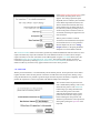
(a) Change the toolbar popup menu setting to Configuration.
(b) Click on the Full Configuration button in the toolbar.
A series of dialogs will appear. Each of these dialogs is described in greater detail in Chapter 2. Please skip
to Chapter 2 if the following outlines are too terse.
• The first series of dialogs ask which input and output channels on the digitizer are being used. Turn on the
check box next to each group of channels then each individual channel that has a cable connected.
• The next dialog is only relevant to electrophysiologists using a patch clamp or microelectrode amplifier
from Axon Instruments, Dagan or Warner. AxoGraph can read and interpret the telegraph signals (gain,
filter frequency, etc.) that are output by these amplifiers. If one or more amplifiers is connected, then
several additional dialogs will appear asking which digitizer channels the telegraph signals are connected
to.
• The next few dialogs request signal names and units for the input and output channels that have cables
connected. The names should clearly distinguish between the various channels, but should not be too long,
because they will be used to label the axes of the data window. If the same name is given to two different
channels, AxoGraph will report an error and repeat the series of dialogs. The signal units should be given
in the most convenient form. For example, if an instrument is measuring a small current then the most
convenient units for the corresponding Analog Input channel may be ‘nA’ (nanoAmps). If an Analog
Output is controlling a fine mechanical positioner, then most convenient units for this channel may be
‘µm’ (micrometers).
5
• The next two dialogs request the gains for the Analog Input and Analog Output channels. The gains can
be specified in either of two different ways. The user can choose the most convenient format. The options
are…
(a) milliVolts at the digitizer per unit at the electronic equipment, or
(b) units at the electronic equipment per Volt at the digitizer.
For example...
An amplifier generates an output signal of 10 mV per nA.
The gain will be either,
10 mV at the Analog Input per nA at the amplifier, or
100 nA at the amplifier per Volt at the Analog Input.
A mechanical translator generates a movement of 0.4 µm per mV of command signal.
The gain will be either,
2.5 mV at the Analog Output per µm at the translator, or
400 µm at the translator per Volt at the Analog Output.
• The next dialog requests the holding levels for the Analog Output channels. Each Analog Output will be
set to the holding level when AxoGraph is launched, and returned to the holding level between periods of
data acquisition. In general, all holding levels should be set to zero.
• The next dialog asks whether the user will ever switch a patch clamp amplifier between voltage-clamp and
current-clamp modes. If the answer is ‘yes’ then a series of dialogs is present that simplifies the task of
switching the amplifier clamp mode. If the answer is ‘no’, then the configuration procedure is complete.
The connections to the digitizer are now fully described. Some additional configuration may be required
before running the data acquisition programs (sampling rate, trigger mode, etc.). Chapters 3 to 9 contain a
detailed description and guide to all the data acquisition programs. Section 1.5 provides a brief overview of
the features available in these programs.
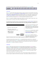
1.4 Trouble-Shoot Hardware and Software Installation
This section presents some common problems and possible solution…
Problem: At start-up AxoGraph reports that it can not find the digitizer
Most probable reason: digitizer has not been correctly installed and connected.
Shut down the computer.
Check that the cable between the digitizer and computer is securely plugged in at both ends.
Check that the digitizer power cable is securely connected.
Make sure the digitizer is switched on, and its front power light is on.
Reboot the computer.
If a Digidata 1320 series digitizer is connected:
Launch the SCSI monitoring application ‘SCSIProbe’ that was installed from the AdvanSys CD.
At the top of the SCSIProbe window there is a popup menu labeled ‘SCSI Buses’
Click on this popup menu. In the list there should be an item labeled ‘AdvanSys…’
If this item does not appear, then the AdvanSys PCI -> SCSI card
has not been installed correctly, or is not working correctly.
Select the item labeled ‘AdvanSys…’
A ‘Digidata 1320’ item should now appear in the list labeled ‘SCSI Devices’
If this item does not appear, then there is a problem with the connection
to the Digidata, or with the Digidata hardware.
If the ‘Digidata 1320’ item does appear then all the hardware is correctly installed and connected.
6
Problem: AxoGraph data acquisition features are not available under the Program menu
Most probable reason: the AxoGraph data acquisition package is not loaded.
Open the AxoGraph 4.9 folder.
Open the folder named Plug-In Programs and confirm that the Acquisition Programs folder is not present.
Search for this folder, then move it into the Plug-In Programs folder
If the Acquisition Programs folder is already present, then there may be more than one copy of AxoGraph
installed on the computer.
Delete the other copies of AxoGraph.
Alternatively, make sure that all AxoGraph aliases point to the latest version.
Launch AxoGraph 4.9
The acquisition programs should now appear under the Program menu.
Problem: AxoGraph data acquisition programs only run in demo mode
Most probable reason: either the digitizer has not been correctly installed and connected (see above), or the
demo version of the data acquisition package is loaded.
To check whether the demo acquisition package is loaded, open the AxoGraph 4.9 folder.
Open the folder named Plug-In Programs and confirm that the Acquisition Programs Demo folder is present.
Drag this folder out of the Plug-In Programs folder.
Search for the folder named Acquisition Programs, then move it into the Plug-In Programs folder.
Launch AxoGraph 4.9
A text box will appear saying that the programs are loading.
If no dialog box appears as the programs are loading, then the acquisition package has found and initialized
the digitizer.
Problem: data acquisition programs run, but do not display the correct signal
Most probable reason: the digitizer is not correctly connected to the electronic equipment, or the acquisition
package is not correctly configured, or the digitizer is not working correctly.
It is important that the electronic equipment and the digitizer reference their electrical signals to the same
ground. This is not usually a problem as most equipment uses the BNC cable outer shield as the signal
ground. However, some amplifiers output a signal that is not referenced to the BNC cable shield, but to a
separate signal ground. They have an external connector (usually labeled ‘signal ground’) that must be
connected to the same ground as the digitizer. Instrutech digitizers have an external connector labeled
‘signal ground’ for this purpose. The Axon Digidata uses the BNC cable earth as its signal ground.
To check the configuration of the AxoGraph data acquisition package …
Select the Configuration popup menu in the toolbar.
Click on the Full Configuration button.
Describe each of the cables that are connected from the electronic equipment to the digitizer.
Make sure that all these cables are actually connected as described.
To check that the digitizer is working correctly…
Disconnect all BNC cables from the digitizer
Connect a cable directly between Analog Output 0 and Analog Input 0
Launch AxoGraph and switch the toolbar popup menu to Scope.
Click on the Run Scope button, then the space-bar to halt the Scope.
Click on Channels button.
Acquire data from Analog Input 0 and direct the test pulse to Analog Output 0.
Click on the Pulse button and enter a large pulse amplitude.
Select Relative time and specify an Onset of 10% and Width of 50%.
Click on the Run Scope button.
Hit the “a” key to autoscale the sweeps. A square pulse should be visible.
7
If a square pulse is NOT displayed, this would indicate a serious problem with the digitizer hardware.
If a square pulse is displayed, this would indicate that everything is working correctly with the AxoGraph
acquisition package and the digitizer hardware. The problem must lie with the electronic equipment, or its
connection to the digitizer.
1.5 Optionally Remove the Electrophysiology Features
Several of the features of the data acquisition package were developed specifically for electrophysiology
research. These include the patch-clamp test pulse, and support for telegraph signals from patch-clamp
amplifiers. If these features are not required, they can be removed to simplify the user interface. Open the
Acquisition Programs folder (in the Plug-In Programs folder). Drag the Electrophysiology folder out of the
Plug -In Programs folder. Quit and re-launch AxoGraph to reset the Program menu and toolbars.
1.6 Summary of Features
• Full support of Axon Digidata 1320 series digitizers and Instrutech ITC-16 and ITC-18 digitizers
Axon Digidata 1320 series
- 16 analog and 4 digital inputs
- 2 analog and 8 digital outputs
- 4 dedicated telegraph inputs
- maximum sample rate of 500 kHz (Digidata 1321A) or 250 kHz (Digidata 1320)
Instrutech ITC series
- 8 analog and 4 digital inputs
- gain control on analog inputs (ITC-18 only)
- 4 analog and 4 digital outputs
- maximum sample rate of 200 kHz
All digitizers
- external trigger can initiate acquisition
- all 16 rear-panel digital input and output channels can be accessed
between episodes using an online analysis command
• Digital storage scope
- measure and display peak amplitude, rise-time, half-width
- ‘hot-keys’ for changing the display range settings on the fly
- AC couple (via baseline subtraction)
- average multiple sweeps
- sweep capture and overlay
- optional output of a test pulse and a trigger pulse during each sweep
- custom analysis program can be applied to every sweep
8
- scope sweeps can be triggered in several different ways...
- at regular user-defined intervals
- locked to the line frequency
- from an external logic signal
- from a signal on an analog input channel
- trigger on amplitude or first-derivative threshold crossings
- display a pre-trigger period
• Digital chart recorder
- scrolling display
- mark events with tags and comments
- optional output of a regular timer or test pulse
- measure and display event frequency
- custom analysis applied during continuous acquisition
• Protocol driven data acquisition
- regular, external or keyboard trigger for episodic data acquisition
- unlimited episode width
- deliver complex waveforms to the analog and digital outputs
- square pulses, trains of pulses and ramps
- incrementing pulse amplitudes and onset times
- arbitrary series of pulse amplitudes from a table
- arbitrary waveform output
- enter a function (exponential, sine wave, etc.)
- convert a recorded signal to an output waveform
- ‘hot-keys’ for initiating predefined protocols
- real-time data analysis during acquisition
- monitor event amplitude or rate versus time
- real-time analysis programs can be customized or extended
- all 16 rear-panel digital input and output channels can be accessed
between episodes using an online analysis command
• Patch-clamp test pulse for electrophysiology research
- measure seal resistance during patch recordings
- measure electrode series resistance, membrane capacitance
and membrane resistance during whole-cell recordings
9
2 Configuration
2.1
2.2
2.3
2.4
2.5
2.6
2.7
2.8
Introduction
Connections
Channel Names
Signal Gains
Holding Levels
Save and Load Configuration
Telegraphs
Clamp Mode
2.1 Introduction
AxoGraph needs to know which input and output channels of the digitizer receive connections. It also needs
to know the gain (amplification) and the units for the signal carried by each connection. AxoGraph uses this
information to scale the input and output signals and to label the axes in the data display windows. There are
five separate programs that can be used to describe the connections and signals: Connections, Channel
Names, Gains, Holding Levels and Telegraphs. The program, Full Configuration, runs each of these five
programs, one after the other. Running all five programs fully describes the connections to the digitizer. If
the connections and the signal gains remain constant, configuration will only need to be performed once
when the data acquisition software is first installed. Signal amplification is the configuration parameter that
is most likely to be altered. When ever the gain of a signal is adjusted, run the Gains program to inform
AxoGraph of the change.
AxoGraph presents a pop-up menu in the toolbar at the bottom-left of the screen. When the Configuration
item is selected in this pop-up menu, a new row of buttons appears in the toolbar. The following sections
describe the function of each of the buttons in the Configuration toolbar.
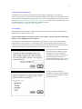
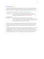
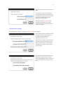
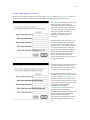
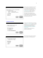
2.2 Connections
The Connections button initiates a series of
dialogs that ask which digitizer channels
have a cable connected. The first dialog
(shown at left) requests an overview of the
connections. This helps to simplify the
subsequent series of dialogs.
10
Next, a series of dialogs request the
connections for the Analog Input channels,
the Analog Output channels, etc. Each of
these dialogs has the same layout as shown
at left for the Analog Outputs dialog.
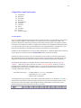
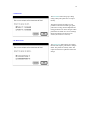
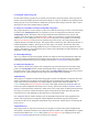
2.3 Channel Names
The Channel Names button initiates a series of dialogs that request signal names for the input and output
channels that have a cable connected. The names should clearly distinguish between the various channels,
because all subsequent dialogs request channels by name, not number. Also, the names should not be too
long because they will be used to label the axes in the data display window. Dialogs are only presented for
channels that have a cable connected (see Section 2.2.). The series of dialogs request signal names for the
Analog Input channels, the Analog Output channels, the Digital Input channels and the Digital Output
channels. A dialog will not appear if there are no cables connected to a group of channels.
The dialogs for the Analog Input and
Analog Output channels also request signal
units. Units should be given in the most
convenient format. For example, if an
instrument is measuring a small current then
the most convenient units for the
corresponding Analog Input signal may be
‘nA’. If an Analog Output signal is
controlling a fine mechanical positioner,
then most convenient units may be ‘µm’.
All four dialogs have the same layout as
shown at left for the Analog Inputs dialog.
11
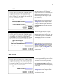
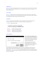
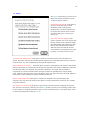
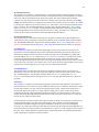
2.4 Signal Gains
The Gains button brings up a series of
dialogs that asks about the signal
amplification or conversion factor for each
of the electronic devices connected to the
digitizer. The first dialog ask how the gains
are to be specified in the subsequent
dialogs. A choice is offered simply for
convenience, because different devices
specify their gains in different ways.
The two subsequent dialogs request the signal gain (amplification and conversion factor) for each Analog
Input and Analog Output channel that has a cable connected. If the gain of an Analog Input or an Analog
Output signal is specified via a telegraph, then that channel will not appear in the gain dialog (see Section
2.7). Two examples follow…
Analog Output Gain
A piezoelectric mechanical positioner
generates a movement of 40 µm per Volt.
The positioner’s command input is
connected to Analog Output 0, and the
signal name and units for this channel are
‘Piezo’ and ‘µm’ (see Section 2.3).
Depending on the option chosen in the first
dialog, the gain will be specified either as
25 mV per µm,
or as 40 µm per V.
12
Analog Input Gain
A voltage-clamp amplifier generates a
signal of 10 mV per pA. The amplifier’s
output is connected to the digitizer at
Analog Input 0, and the signal name and
units for this channel are ‘Current’ and ‘pA’
(see Section 2.3).
Depending on the option chosen in the first
dialog, the gain will be specified either as
10 mV per pA,
or as 100 pA per Volt.
2.5 Holding Levels
The Holding Levels button brings up a
dialog that requests the level at which to
hold the signal on each of the active Analog
Output channels (those that have a cable
connected). Any command signals sent to
an Analog Output will be superimposed on
the holding level. For most purposes, the
holding levels will be set to zero as shown
at left.
The signals on the active Analog Output
channels will be set to the requested holding
levels immediately after clicking OK in this
dialog. All output channels will be set to their holding levels when AxoGraph is launched, and at the
termination of an acquisition protocol (see Chapter 6, ‘Protocol Driven Data Acquisition’). Scope and Chart
test pulses will be superimposed on the holding level of the pulse output channel.
13
2.6 Save and Load Configuration
A mechanism is provided for switching quickly between different configurations of the digitizer
connections. This feature is useful when the instruments connected to the digitizer are changed between two
or more standard configurations on a regular basis. A set of connection parameters can be saved to a file by
selecting, Program ➔ Acquisition Options ➔ Save Configuration. The file is saved in the same folder as the
AxoGraph application. A set of parameters can be loaded by selecting,
Program ➔ Acquisition Options ➔ Load Configuration.
2.7 Telegraphs
The telegraphs feature is relevant to electrophysiologists using a patch clamp amplifier manufactured by
Axon Instruments, Dagan, Warner or NPI.
If a patch clamp amplifier is not being used then review Section 1.5, ‘Removing the Electrophysiology
Features’, before skipping forward to Chapter 3.
AxoGraph can read and interpret the telegraph signals (gain setting, etc.) that are output by most patch
clamp amplifiers. Most importantly, it can adjust the gain of the specified input signal according to the
voltage on the gain telegraph channel. Other supported signals include the AxoPatch voltage-clamp mode
telegraph, filter frequency telegraph and whole-cell capacitance compensation telegraph.
For experiments involving simultaneous
presynaptic and postsynaptic recording,
there may be two or more amplifiers
connected to the digitizer. AxoGraph can
support telegraphs from up to four
amplifiers simultaneously. The Telegraphs
button brings up the dialog shown at left.
The next two dialogs request the
manufacturer of the patch clamp amplifier
(shown at left) and the amplifier’s model
number (not shown).
14
Gain Telegraph
Next, one or more dialogs appear asking for
the channel that each of the telegraph
signals is connected to. The first dialog asks
about the gain telegraph connection. For
Instrutech digitizers, the telegraph signal
must be connected to an ADC input channel
(as shown at left).
Before each trace is acquired the signal on
Analog Input 7 will be sampled, and the
voltage will be used to adjust the gain for
the signal on Analog Input 0. This is the
Scaled Output signal from the patch clamp
amplifier.
The gain telegraph dialog has a slightly
different format when the digitizer is a
Digidata 1320 series (as shown at left). This
is because the Digidata has four dedicated
telegraph input channels on the rear panel.
Telegraph signals must be connected to
these channels.
Before each trace is acquired the signal on
Rear Panel Telegraph 0 will be sampled,
and the voltage will be used to adjust the
gain for the signal on Analog Input 0. This
is the Scaled Output signal from the patch
clamp amplifier.
Mode Telegraph
The next dialog only appears if the amplifier
is an AxoPatch 200. This amplifier supports
a Mode telegraph which signals whether the
AxoPatch is in current-clamp or voltageclamp mode. Both the Scaled Output and
the External Command connections on the
AxoPatch change their behaviour depending
on the mode.
Before each trace is acquired the signal on
Analog Input 6 will be sampled, and the
voltage will be used to determine the
AxoPatch clamp mode.
15
The units and gain setting for the AxoPatch
External Command connection will be
interpreted as either a current command or a
voltage command depending on the
AxoPatch recording mode. The next dialog
asks which Analog Output channel is
connected to the External Command
signal. The signal units will be adjusted to
‘pA’ for current-clamp, or ‘mV’ for voltageclamp.
The Mode Telegraph also adjusts the units for the signal connected to the AxoPatch Scaled Output. If the
gain telegraph is active, then the Scaled Output channel has already been specified (see Gain Telegraph
dialog above), so no dialog is presented. However, if the gain telegraph is not active, then dialog appears
asking which Analog Input channel is connected to the Scaled Output signal. The units of the specified
channel will be adjusted to ‘mV’ for current-clamp, or to ‘pA’ for voltage-clamp.
Frequency and Capacitance Telegraphs
The next dialog only appears if filter
frequency or cell capacitance telegraphs are
supported by the patch clamp amplifier.
Before each trace is acquired the signal on
Analog Input 5 will be sampled, and the
voltage will be used to determine the
amplifier's filter frequency setting. This
setting will be stored in the Notes section of
the acquired data file.
16
2.8 Clamp Mode
The Clamp Mode feature is only relevant to electrophysiologists using a voltage-clamp amplifier (other than
an AxoPatch 200B) that is occasionally switched between current- and voltage-clamp modes. The AxoPatch
200B has a mode telegraph output that signals a change of clamp mode. When this telegraph is used, the
Clamp Mode program is not needed, and is removed from the Configuration toolbar. Most other voltageclamp amplifiers have only a single connection for an External Command signal. The signal is interpreted
as a voltage command when the amplifier is in voltage-clamp mode, and as a current command when the
amplifier is in current-clamp mode. The gain and unit settings for the Analog Output channel that generates
the External Command signal, will change when the clamp mode is changed. In addition, some amplifiers
have a Scaled Output signal that reports the holding current when the amplifier is in voltage-clamp mode,
and the membrane potential when the amplifier is in current-clamp mode. The gain and unit settings for the
Analog Input channel that receives the Scaled Output signal, will change when the clamp mode is
changed.
The Clamp Mode button can be used to inform the acquisition program that the clamp mode has changed.
AxoGraph then makes all the necessary changes to the configuration settings for the External Command
and Scaled Output channels.
The dialog shown at left indicates that the
amplifier is now operating in voltage-clamp
mode.
The Clamp Mode program will only work if
the configuration programs Connections and
Channel Names have already been run, and
the External Command signal has been
described.
The first time the Clamp Mode program is run, it is necessary to enter the gain and unit settings for the
External Command signal in current- and voltage-clamp modes. Selecting the Edit Clamp Mode Parameters
option in the previous dialog then clicking OK, brings up a series of dialogs that request the mode switch
parameters.
The first dialog asks which Analog Output
channel is connected to the External
Command of the voltage-clamp amplifier.
The channels are listed by name.
17
The second dialog requests the units for the
voltage and current clamp commands. These
will generally be ‘mV’ for the voltage
command and either ‘pA’ or ‘nA’ for the
current command.
The third dialog requests the gains for the
voltage and current clamp commands. The
gains are given in mV of voltage-clamp
command per Volt at the Analog Output,
and in pA of current-clamp command per
Volt at the Analog Output.
The fourth dialog asks which Analog Input
receives the amplifier’s Scaled Output
signal. This signal will report current when
in voltage-clamp mode, and membrane
potential when in current-clamp mode.
If a gain telegraph is active, then the Scaled
Output channel has already been specified
(see Gain Telegraph dialog above), so this
dialog will not be presented.
The fifth dialog asks for the signal names to
be used for the Scaled Output channel
when in voltage-clamp mode and currentclamp mode.
18
3 Digital Oscilloscope
3.1
3.2
3.3
3.4
3.5
3.6
3.7
3.8
3.9
3.10
3.11
3.12
Introduction
Run Scope
Hot Keys
Display
Average
Timebase
Trigger
Channels
Gains
Test Pulse
Analyse
Custom Analysis
3.1 Introduction
The Scope program implements all the main features of a storage oscilloscope. It is designed for monitoring
an intermittent electrical signal. Each time the scope is triggered, an electrical signal is plotted versus time in
the scope window. The displayed waveform is termed a ‘sweep’. Successive sweeps can be overlaid (storage
mode), and erased manually. Alternatively, the window can be erased automatically before displaying each
new sweep. Sweeps can be triggered from an external pulse, or they can be triggered at regular intervals by
the computer. There is a ‘line trigger’ mode that synchronizes the start of each sweep with the power line
frequency (50 or 60 Hz). A single sweep can be ‘captured’ and overlaid on later sweeps. Signals on up to 8
channels can be displayed simultaneously.
Signal waveforms are displayed, but are not saved to disk. See Chapter 4, ‘Digital Chart Recorder’, or
Chapter 5, ‘Protocol Driven Data Acquisition’ for programs that can save the acquired signals to disk.
In addition to the standard storage scope features outlined above, AxoGraph's digital scope can average a
signal over multiple sweeps and display the running average. It can send a synch pulse to a Digital Output
at the beginning of each sweep, and a test pulse to an Analog Output during each sweep. It can also
measure and display the peak amplitude, rise-time and width of an event in each sweep.
AxoGraph presents a pop-up menu in the toolbar at the bottom-left of the screen. When the Scope item is
selected in this pop-up menu, a new window titled Scope Window will appear. The following sections
describe the function of each of the buttons in the Scope toolbar.
3.2 Run Scope
The Run Scope button starts the digital scope. A series of sweeps will be displayed in the scope window.
Hitting the space-bar on the keyboard halts the scope.
The rate at which the traces appear will depend on how the sweeps are triggered. The various trigger options
are described in Section 3.7, below.
19
3.3 Hot Keys
The Hot Keys button opens a documentation window which describes keyboard shortcuts for controlling the
digital oscilloscope. Here is the list of the scope hot keys, and their actions.
space-bar : halts the scope
a:
f:
c:
e:
Automatically adjust Y axis range to the size of the signal
Adjust Y axis to display the full Analog Input range
Capture a trace for comparison with subsequent traces
Erase the scope
(useful when the Erase between sweeps option is turned off)
up-arrow :
down-arrow :
right-arrow :
left-arrow :
increase Y-axis range (zoom out)
decrease Y-axis range (zoom in)
increase sweep width
decrease sweep width
The following keys modify the Scope test pulse.
+ : increase pulse amplitude
- : decrease pulse amplitude
i : Invert pulse
The following keys are active when using an internal trigger.
(The test pulse in inactivated in this trigger mode.)
+ : increase trigger level
- : decrease trigger level
3.4 Display
The Display button in the Scope toolbar
brings up the Scope Display Settings dialog.
This asks whether to display information
about the acquisition parameters in the
scope window. It also asks how sweeps are
to be displayed.
Erase Between Sweeps
When this check box is turned off, each new
sweep is overlaid on preceding sweeps. This
emulates the behavior of a storage
oscilloscope. Typing the letter "e" while the
scope program is running erases the scope
window. When this check box is turned on,
the scope is erased before each new trace is
displayed. This emulates the behavior of a
standard oscilloscope.
Subtract Baseline (AC Couple)
When this check box is turned on, the signal
amplitude is calculated over a short interval
20
at the start of each sweep. This ‘baseline’ amplitude is subtracted from the signal before it is displayed. This
procedure emulates the ‘AC couple’ option available on electronic oscilloscopes. It is useful in situations
where the signal of interest is superimposed on a larger drifting signal. It stabilizes the signal at the center of
the display range.
Show Pulse Size
When this check box is turned on, the amplitude of the test pulse is displayed in the scope window.
Show Sample Rate
When this check box is turned on, the acquisition sample rate is displayed in the scope window.
Auto-Scale Scope
When this check box is turned on, the Y axis display range of the scope window is automatically adjusted to
display the full amplitude of each signal (auto-scale). The auto-scale function is performed periodically. The
interval between each auto-scale can be entered in the Sweeps Between Auto-Scale field. When the AutoScale Scope check box is turned off, the auto-scale function can be performed at any time by typing the
letter "a" while the scope program is running (see Section 3.3, ‘Hot-Keys’).
3.5 Average
The Average button brings up the dialog
shown at left.
When the Average Sweeps check box is on,
a running average of successive sweeps is
calculated and displayed in the scope
window. This is useful for improving the
signal-to-noise characteristics of the
displayed signal.
3.6 Timebase
The Timebase button in the Scope toolbar
brings up the dialog shown at left. This
dialog controls the sample rate used by the
Scope program to acquire signals. When
several input channels are active, the signal
on each channel will be sampled at the
requested rate. This dialog also controls the
width of each sweep in milliseconds.
The sample rate should be at least twice the
highest frequency of interest in the signal.
The best results are obtained when the
signal is low-pass filtered at a frequency
equal to half the sample rate.
21
Because of limitations in the digitizer hardware, it is not always possible to sample data points exactly at the
requested sample rate. See Section 11.2, ‘Hardware Limitations on the Sampling Rate’ for a discussion of
these limitations.
3.7 Trigger
The Trigger button in the Scope toolbar
brings up the Scope Trigger Mode dialog.
This dialog controls how sweeps are
initiated (triggered). The are four options....
Regular
When this mode is selected, sweeps are
initiated at a regular interval that is specified
in a subsequent dialog (not shown). If the
sweep start-to-start time is set to zero,
sweeps will be initiated as rapidly as
possible. If Scope can not keep up with the
requested sweep start-to-start time, a
warning dialog will appear when the
program is halted.
Internal
When this mode is selected, sweeps are initiated whenever a signal on one of the Analog Input channels
crosses a specified threshold. The procedure for setting the threshold is described below.
External
When this mode is selected, sweeps are initiated whenever a 5 Volt signal appears on the digitizer connector
labeled Trigger Input. This permits the start of the scope sweep to by synchronized with an external event.
Line
When this mode is selected, sweeps will be synchronized with the power line voltage cycle. The Axon
Digidata 1320 series incorporates a hardware line trigger. The Instrutech ITC series need to be triggered
from software, so a second dialog appears asking whether the power line frequency is 50 or 60 Hz. Sweeps
will be initiated at the shortest possible interval that is a multiple of 20 ms (for 50 Hz line) or 16.6666 ms
(for 60 Hz line). The ‘line’ trigger mode is useful when testing for contamination of a signal by power line
noise. It can be used in conjunction with sweep averaging to improve sensitivity (see Section 3.5 above).
22
When Internal triggering is selected, a series of three dialogs appears that request additional information
about when to initialize each sweep. The first dialog (not shown) asks which Analog Input channel carries
the signal that will be used to trigger the sweeps. This can be any of the connected signals. Typically, one of
the signals being displayed in the scope window will be used as the trigger signal.
The next dialog asks whether to initiate a
sweep when the signal amplitude crosses a
threshold level, or when the slope of the
signal exceeds a threshold level.
If Amplitude Threshold is selected, the next
dialog requests the direction of threshold
crossing (low-to-high or high-to-low) that
initiates the sweep. It also requests the
threshold level that must be crossed.
The signal can optionally be displayed both
before and after the threshold crossing event
that triggers the sweep. This is achieved by
setting the Pre-Trigger Interval to a value
greater than zero.
If Slope Threshold is selected, the next
dialog requests the range over which to
calculate the slope, and the slope threshold
level that initiates the sweep.
The slope of the signal is calculated by
fitting a line over the specified calculation
range. This calculation is continuously
updated as the signal is acquired, until the
slope exceeds the specified threshold. If the
Trigger Level is set to a negative value, then
a sweep will be triggered when the slope of
the signal is more negative than the
threshold. This permits triggering on
negative-going events.
23
3.8 Channels
The Channels button in the Scope toolbar
initiates a series of three dialogs. The first
dialog asks which Analog Input and
Digital Input signals to display in the scope
window. Only channels that have a cable
connected are listed (see Section 2.2,
‘Connections’). Channels are listed by
name, not by number (see Section 2.3,
‘Channel Names’).
When two or more input channels are
selected, the signals will be displayed by
default in separate groups within the scope
window. The signals from multiple channels
can be overlaid by selecting either Combine or Group under the Trace menu. Channels should only be
combined if their signals have the same units (e.g. mV).
The digital scope can optionally deliver a
test pulse to one Analog Output or Digital
Output channel during each sweep. The
second dialog asks which channel (if any) is
to receive the test pulse.
The duration and amplitude of the test pulse can be edited via the Pulse button in the Scope toolbar (see
Section 3.10 below).
The scope can optionally deliver a brief
synchronizing pulse to a Digital Output
channel every time a sweep is triggered.
This pulse could be used to trigger a
waveform generator, or an electronic
oscilloscope for example. The third dialog
asks which channel (if any) is to receive the
synch pulse.
24
3.9 Gains
The Gains button in the Scope toolbar brings up two dialogs that request the signal gain (amplification and
conversion factor) for each Analog Input and Analog Output channel. These dialogs are described in detail
in Section 2.4, ‘Signal Gains’. The Gains button is also found in the Configuration toolbar, but is duplicated
in the Scope and Chart toolbars for convenience.
3.10 Test Pulse
The digital scope can optionally deliver a test pulse to one Analog Output or Digital Output channel
during each sweep (see Section 3.8, ‘Channels’). If a test pulse channel has been selected, then the Pulse
button in the Scope toolbar brings up a series of three dialogs requesting the amplitude, onset time and
duration of the test pulse.
The first dialog only appears if an Analog
Output channel has been selected. It asks
for the pulse amplitude.
The pulse amplitude can also be adjusted
using ‘Hot Keys’ (see Section 3.3).
The second dialog asks whether the onset
and duration are to be specified in fixed
time units (ms), or as a fraction of the sweep
width.
If fixed time units are specified, then the
third dialog requests the pulse onset time
and pulse width in milliseconds (not shown).
The test pulse duration will remain constant
even if the scope sampling rate and sweep
width settings are changed.
If relative timing is selected, the test pulse
will change in duration when the sweep
width is changed. The pulse will always
occupy the same fraction of the sweep, and
the third dialog asks which fraction that will
be.
25
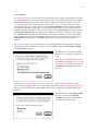
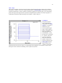
3.11 Analyse
The Analyse button in the Scope toolbar
presents the online analysis dialog. The
digital scope optionally analyses each
sweep immediately after it is acquired, and
displays the results overlaid with the sweep.
Three standard analysis programs identify
the largest event in each episode, and
analyse that event. They optionally measure
the peak amplitude, the 20-80% rise-time
and the half-width of the event. Custom
analysis programs can also be run before the
first sweep, and after every sweep. For
example, the program ‘CustomNoiseSD’
calculates the standard deviation of the
signal in the baseline region before the start
of the test pulse. The code for this program
can be found in the file named ‘Custom
Analysis’ which is located in the
‘Acquisition’ sub-folder of the ‘Acquisition
Programs’ folder.
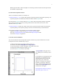
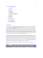
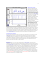
When the digital scope is run with
online analysis active, the scope
window will display the results
superimposed on each sweep. The
figure at left shows a single Scope
sweep with the peak amplitude, the risetime, and the noise SD analysis results
superimposed. The noise SD was
calculated and displayed by a custom
analysis program which is described
below.
26
3.12 Custom Analysis
Custom analysis programs can be run before the first sweep, and after every sweep. A program run before
the first sweep would typically set up global parameters that control subsequent analysis. For information
about writing a programs in AxoGraph, see the chapter on programming in the AxoGraph User Manual.
Two example online Scope analysis programs are supplied with AxoGraph. They are..
CustomNoiseSD:
Calculates and displays the standard deviation (SD) of the signal over the
first 10% of each sweep. To activate the program, bring up the Analyse dialog and
enter the name ‘CustomNoiseSD’ in the ‘After Every Sweep’ field.
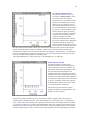
ScopeSpectrumSetup,
ScopeSpectrum:
calculates the power spectrum of the signal in each sweep and displays
the result in a separate window on log-log axes. To activate the program, bring up the
Analyse dialog and enter the name ‘ScopeSpectrumSetup’ in the ‘Before First Sweep’
field and ‘ScopeSpectrum’ in the ‘After Every Sweep’ field.
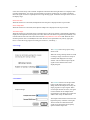
The source code for the ‘CustomNoiseSD’ analysis program is presented on the next page. This code can
also be found in the file named ‘Custom Analysis’ which is located in the ‘Acquisition’ sub-folder of the
‘Acquisition Programs’ folder. It should be a useful starting point for writing simple custom analysis
programs.
The ‘CustomNoiseSD’ program is automatically loaded when AxoGraph is launched, because it is located in
a sub-folder of the Plug-In Programs folder. When a new custom analysis program is written, it can be
loaded and tested as follows. First, save the new custom analysis program in the Plug-In Programs folder or
sub-folder. Next, select the AxoGraph menu item Program ➔ Reload Plug-Ins. Finally, enter the custom
analysis program name in the After Every Sweep field of the online analysis dialog (as shown above).
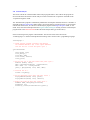
27
Source code listing for the program ‘CustomNoiseSD’. The first line of the source file must be
‘LocalLanguage C’ to inform AxoGraph that the following code is written in the C programming language.
localLanguage C
/* Custom analysis program calculates and displays
the standard deviation (SD) of the signal measured
over the first 10% of each sweep */
void CustomNoiseSD
{
short window, trace;
float yArray[0];
float xMin, xMax;
float noiseSD, theScale;
string yUnits;
/* Get the front window and trace number */
GetFront (window, trace);
GetXRange (window, xMin, xMax);
/* Get the baseline region before the start of the test pulse */
xMax = startPulsePnt * sampleInterval;
yArray = yRange(window, trace, 0, xMax);
/* Make sure we got at least 3 points */
if (ArraySize(yArray) > 2) {
/* Calculate the SD */
noiseSD = SD(yArray);
/* Get the displayed Y-axis units and scale factor */
DisplayedYUnits(window, trace, yUnits);
DisplayedYScale(window, trace, theScale);
/* Move to a point just below the baseline */
DrawMove (xMin, Mean(yArray)-2*noiseSD);
DrawPixelMove (5, 12);
DrawSetSize (12);
/* Display the noise SD (in Y-axis units) */
DrawString (concat(noiseSD*theScale:3,yUnits));
}
}
28
4 Digital Chart and Tape Recorder
4.1
4.2
4.3
4.4
4.5
4.6
4.7
4.8
4.9
4.10
4.11
Introduction
Run Chart
New Chart
Hot Keys
Event Markers
Timebase
Channels
Gains
Test Pulse
Analyse
Custom Analysis
4.1 Introduction
The Chart program implements all the main features of a chart recorder. It can continuously acquire data at
audio rates (up to 50 kHz on some computers) so it could also be used as a digital tape recorder. The
program is designed for continuously monitoring and recording electrical signals. The signals are plotted
versus time in a scrolling chart window. The digital chart recorder can be stopped and restarted many times
in a single recording session. The gain and sampling rate can be changed during a recording session. The
chart can be annotated at any time during the recording with comments and event markers.
In addition to the standard features of a chart recorder outlined above, AxoGraph's digital chart recorder can
send a regular test or stimulus pulse to an Analog Output during continuous recording.
Chart data is acquired to memory, and is not automatically written to disk. To write the acquired data to
disk, the chart file must be saved manually. This can be done at any time during a recording session. The
digital chart recorder will halt with an error message when all available system memory is exhausted.
The maximum chart length can be estimated as follows. Switch to the Finder, and select About This
Computer… under the Apple menu. Note the size of the Largest Unused Block of memory. If Chart is
recording from N channels, then AxoGraph requires 4 x (N+1) bytes per sample point, and 4 x (N+1) x
SampleRate bytes per second. For example, if there is 36 MBytes of memory available, and Chart is
recording 2 channels at 1 kHz, then...
Maximum Chart Length = Available Memory / (4 x (N+1) x SampleRate)
= 36,000,000 / (4 x (2+1) x 1,000)
= 3,000 seconds or 50 minutes
AxoGraph presents a pop-up menu in the toolbar at the bottom-left of the screen. When the Chart item is
selected in this pop-up menu, a dialog will appear asking for the file name and destination folder for the
chart data file. A new chart window will then appear with the selected name. The following sections
describe the function of each of the buttons in the Chart toolbar.
29
4.2 Run Chart
The Run Chart button starts the digital chart recorder. The signal on one or more channels will be displayed
in the scrolling chart window. Hitting the space-bar on the keyboard stops the chart. Clicking the Run Chart
button restarts the chart.
4.3 New Chart
The New Chart button first closes the old chart window (if one is open), then opens a new chart window.
The user is given the option of saving or discarding the old chart data. The new chart file name is generated
by incrementing the sequence number at the end of the file name.
4.4 Hot Keys
The Hot Keys button opens a documentation window with information about keyboard shortcuts for
controlling the digital chart recorder. Here is a list of the chart hot keys, and their actions.
space-bar : halts the chart recorder
a : Auto-adjust Y axis range to the size of the signal
f : Adjust Y axis to display the full Analog Input range
t : Add an event marker (tag) and a comment to the chart
up-arrow :
down-arrow :
left-arrow :
right-arrow :
increase Y-axis range (zoom out)
decrease Y-axis range (zoom in)
increase the time range (zoom out)
decrease the time range (zoom in)
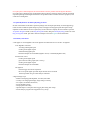
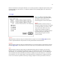
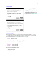
4.5 Event Markers
The action of the event marker (tag) hot
key, "t", depends on the sample rate and the
size of the internal buffer in the digitizer. If
the buffer will not overflow in the next few
seconds, then a dialog appears asking for a
comment describing the event.
The dialog indicates how long there is
before the buffer overflows. If there is
insufficient time to enter a comment, then a
tag is added without an associated
comment.
Tags are displayed as vertical dashed lines in the chart window. Tag comments are stored in the chart
window's Notes, together with the time that the event occurred. These comments can be accessed by
selecting Display ➔ Comments and Notes, or by clicking the Note button in the vertical toolbar at the left of
the chart window. If the chart is halted and restarted, the stop and start times will be included automatically
in the list of event markers.
30
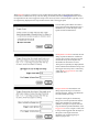
4.6 Timebase
The Timebase button in the Chart toolbar
brings up the dialog shown at left. This
dialog controls the sample rate used by the
Chart program to acquire signals. When
several input channels are active, the signal
on each channel will be sampled at the
requested rate. The sample rate should be at
least twice the highest frequency of interest
in the signal. The best results are obtained
when the signal is low-pass filtered at a
frequency equal to half the sample rate.
This dialog also controls the length of the
chart record. The chart recorder will halt
automatically when the record reaches the length specified in the Record Length field. For example, the
above dialog requests a 20 minute recording (20 x 60 = 1200 sec). If the Record Length is set to zero, then
recording will continue until all available system memory is full.
Because of limitations in the digitizer hardware, it is not always possible to sample data points exactly at the
requested sampling rate. See Section 11.2, ‘Hardware Limitations on the Sampling Rate’ for a discussion of
these limitations.
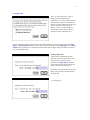
4.7 Channels
The Channels button in the Chart toolbar
brings up two dialogs. The first dialog asks
which Analog Input and Digital Input
signals to display in the chart window. Only
channels that have a cable connected are
listed (see Section 2.2, ‘Connections’).
Channels are listed by name, not by number
(see Section 2.3, ‘Channel Names’).
When two or more input channels are
selected, the signals will be displayed by
default in separate groups within the chart
window. The signals from multiple channels
can be overlaid by selecting either Combine
or Group under the Trace menu. In general, channels should only be combined if their signals have the same
units (e.g. mV).
31
The digital chart recorder can optionally
deliver a regular test pulse to one Analog
Output or Digital Output channel. The
second dialog asks which channel (if any) is
to receive the regular test pulse.
The frequency, duration and amplitude of the test pulse can be edited via the Pulse button in the Chart
toolbar (see Section 4.9 below).
4.8 Gains
The Gains button in the Chart toolbar brings up two dialogs that request the signal gain (amplification and
conversion factor) for each Analog Input and Analog Output channel. These dialogs are described in detail
in Section 2.4, ‘Signal Gains’. The Gains button is also found in the Configuration toolbar, but is duplicated
in the Scope and Chart toolbars for convenience.
4.9 Test Pulse
The digital chart recorder can optionally
deliver a regular test pulse to one Analog
Output or Digital Output channel during
continuous recording (see Section 4.7,
‘Channels’). If a test pulse channel has been
selected, then the Pulse button in the Scope
toolbar brings up a series of three dialogs
requesting the time between test pulses, and
their amplitude and duration. The first
dialog only appears if an Analog Output
channel has been selected. It asks for the
pulse amplitude.
32
The second dialog asks for the onset time to
the first pulse, the time between subsequent
pulses, and the duration (width) of each
pulse.
4.10 Analyse
The Analyse button in the Chart toolbar
brings up the online analysis dialog. The
chart recorder optionally runs a custom
analysis program after each test pulse cycle
(see Section 4.9, ‘Test Pulse’). A custom
analysis programs can also be run before the
first pulse, and would typically set up global
parameters that control subsequent analysis.
For information about writing a custom
analysis program, see the chapter on
programming in the AxoGraph Online
Manual.
33
4.11 Custom Analysis
The source code for the ‘ChartNoiseSD’ online analysis program follows. The code for this program can
also be found in the file named ‘Custom Analysis’ which is located in the ‘Acquisition’ sub-folder of the
‘Acquisition Programs’ folder.
The ‘ChartNoiseSD’ program is automatically loaded when AxoGraph is launched, because it is located in a
sub-folder of the Plug-In Programs folder. When a new custom analysis program is written, it can be loaded
and tested as follows. First, save the new custom analysis program in the Plug-In Programs folder, or subfolder. Next, select the AxoGraph menu item Program ➔ Reload Plug-Ins. Finally, enter the custom analysis
program name in the After Each Pulse field of the online analysis dialog (as shown above).
Source code listing for the program ‘ChartNoiseSD’. The first line of the source file must be
‘LocalLanguage C’ to inform AxoGraph that the following code is written in the C programming language.
LocalLanguage C
/* Custom analysis program calculates and displays
the standard deviation (SD) of the signal measured
over the last 10% of each test pulse cycle */
void ChartNoiseSD
{
short window, trace;
float yArray[0];
float xMin, xMax;
float noiseSD, theScale;
string yUnits;
/* Get the last 10% of the most recent test pulse cycle */
GetFront (window, trace);
xMax = ChartCumulativePoints * sampleInterval;
xMin = xMax - 0.1 * PulseCycleTime;
yArray = yRange(window, trace, xMin, xMax);
/* Calculate the SD */
noiseSD = SD(yArray);
/* Get the displayed Y-axis units and scale factor */
DisplayedYUnits(window, trace, yUnits);
DisplayedYScale(window, trace, theScale);
/* Display the noise SD using the Y-axis units */
DrawMove (xMax, Mean(yArray)+6*noiseSD);
DrawSetSize (12);
DrawString (concat(noiseSD*theScale:3,yUnits));
}
34
5 Electrophysiology Test Pulse
5.1
5.2
5.3
5.4
5.5
5.6
5.7
5.8
5.9
Introduction
Test Channels
Test Pulse Hot Keys
Test Seal
Test Cell
Test To Log
Test Setup
Test Pulse
Test Link
5.1 Introduction
The Test Seal and Test Cell programs are designed to help electrophysiologists set up and perform patchclamp or voltage-clamp experiments.
If the data acquisition software will not be used for electrophysiology experiments, then review
Section 1.5, ‘Removing the Electrophysiology Features’, before skipping forward to Chapter 6.
The Test Seal program monitors the input resistance of a patch recording electrode. This is useful for
checking the electrode is OK when it is first lowered into extracellular solution, and for monitoring the
formation of a GOhm seal. The program delivers a series of small voltage-clamp pulses (typically 1-10 mV),
and monitors the clamp current in a scope window. The electrode input resistance is calculated and
displayed in the scope window, overlaid on the trace. The input resistance can also be directed to the log
window.
The Test Cell program monitors three electrical parameters when recording in whole-cell voltage-clamp
configuration. These are the membrane capacitance and input resistance of the cell, and the series resistance
of the electrode. The program delivers a series of small voltage-clamp pulses, and monitors the current in a
scope window. The three parameters are calculated from the shape of the response, and displayed in the
scope window, overlaid on the trace. The value of the three parameters can also be directed to the log
window.
AxoGraph presents a pop-up menu in the toolbar at the bottom-left of the screen. When the Test Pulse item
is selected in this pop-up menu, a new window titled Test Pulse Window will appear. The following sections
describe the function of each of the buttons in the Test Pulse toolbar.
35
5.2 Test Channels
The Test Channels button brings up two
successive dialogs that define which
Analog Input channel is connected to the
voltage-clamp current signal, and which and
Analog Output channel is connected to the
voltage-clamp command signals. This must
be done before using Test Seal or Test Cell.
5.3 Test Pulse Hot Keys
Hot keys can be used to modify the scope display and the test pulse amplitude while the Test Seal or Test
Cell program is running. They are a subset of the scope hot keys, described in Section 3.3. To display hotkey information, switch to the Scope toolbar and click on the Hot Key button.
space-bar : halts the test program
a : Automatically adjust Y axis range to the size of the signal
f : Adjust Y axis to display the full Analog Input range
up-arrow :
down-arrow :
right-arrow :
left-arrow :
increase Y-axis range (zoom out)
decrease Y-axis range (zoom in)
increase sweep width
decrease sweep width
The following keys modify the test pulse size.
+ : increase pulse amplitude
- : decrease pulse amplitude
i : Invert pulse
36
5.4 Test Seal
The Test Seal button
activates the scope
window that monitors the
recording electrode input
resistance, or seal
resistance. A series of
voltage-clamp pulses is
delivered, and the current
response is monitored. The
amplitude of the voltageclamp pulse, and the seal
resistance are displayed at
the bottom of the scope
window. Hitting the spacebar on the keyboard halts
the scope.
The electrode input
resistance is calculated
from the amplitude of the response to each voltage-clamp pulse. The amplitude is measured by averaging
the current over the last half of the pulse response, as indicated by the horizontal red line superimposed on
the current response. The amplitude is measured relative to the baseline current before the start of the
response, as indicated by the horizontal dashed green line.
5.5 Test Cell
The Test Cell button
activates the scope window
that monitors the electrode
series resistance and the
whole-cell membrane
capacitance and input
resistance. A series of
voltage-clamp pulses is
delivered, and the current
response is monitored. The
amplitude of the pulse, and
the passive electrical
parameters are displayed at
the bottom of the scope
window. Hitting the spacebar on the keyboard halts
the scope.
The passive electrical
parameters are calculated
by measuring the steadystate current at the end of
each pulse response, then
fitting an exponential to the
first few milliseconds of the response. The fitted exponential and steady-state amplitude are shown as a red
37
line superimposed on the current response. The amplitude is measured relative to the baseline current before
the start of the response, as indicated by the horizontal dashed green line.
Several factors will influence the reliability of the Test Cell parameter estimates. It is important that the
sampling rate and low-pass filter frequency permit the current decay to be captured without distortion. Also,
the test pulse should be long enough for the current response to decay to a steady-state level.
Test Cell will provide a reliable estimate of series resistance and input resistance under most circumstances.
Test Cell only provides an accurate estimate of the total membrane capacitance when a cell is ‘isopotential’.
In practice this is only true when a cell has no processes (dendrites, axon, etc.), or when the processes are
very short or fine. When a cell is isopotential, the current response decays as a single exponential, permitting
and accurate estimate of membrane capacitance. If large dendrites or other processes are present, the current
decay will follow a multi-exponential time course, because the membrane capacitance is ‘distributed’ along
the dendrites. This makes it very difficult to calculate whole-cell capacitance. If the exponential fit is
restricted to the first millisecond or so of the response, then the reported capacitance value may represent a
useful approximation of the membrane capacitance of the cell body minus the processes. The reported
capacitance value will depend on the time range over which the exponential or double-exponential function
is fit. This can be adjusted via the Test Setup button, as described in Section 5.7, below.
5.6 Test To Log
The Test To Log button activates either the Test Seal or the Test Cell scope window, whichever was most
recently active. When the scope is halted by hitting the space-bar, the parameter values that are displayed in
the scope window will be appended to the log window. The time that the measurement was made will also
be noted in the log.
5.7 Test Setup
The Test Setup button brings up two dialogs that adjust the behavior of Test Seal and the Test Cell
programs.
Increasing the Pulses per Computation will
improve the reliability of the parameter
estimates, but will cause the scope window
to update more slowly.
38
A single exponential fit is only suitable for a
spherical cell, or a cell with very short, fine
process (dendrites, axon, etc.). For most
neurons, the current response will decay
with a multi-exponential time course, and a
double-exponential fit will provide a more
accurate estimate of membrane capacitance.
Even if the Fit Double Exponential option is
on, AxoGraph will automatically revert to a
single-exponential fit when appropriate.
5.8 Test Pulse
The Test Pulse button brings up a series of three dialogs requesting the amplitude, onset time and duration of
the test pulse. These dialogs are described in detail in Section 3.10, ‘Test Pulse’. The pulse amplitude can
also be adjusted using ‘Hot Keys’ (see Section 3.3).
The first dialog requests the pulse amplitude. The second dialog asks whether the onset and duration are to
be specified in fixed time units (milliseconds), or as a fraction of the sweep width. If fixed time units are
specified, then the third dialog requests the pulse onset time and pulse width in milliseconds. The test pulse
duration will remain constant even if the scope sampling rate and sweep width settings are changed. If
relative timing is selected, the test pulse will change in duration when the sweep width is changed. The pulse
will always occupy the same fraction of the sweep, and the third dialog asks which fraction that will be.
5.9 Test Link
The Test Link feature provides a mechanism for noting the test pulse results to the log window then
immediately running a data acquisition protocol. The Test Link button brings up a dialog that requests the
file name of an acquisition protocol (see Chapter 6 for an explanation of protocol files). When the Test To
Log program is halted by hitting the space-bar, the test results will be directed to the log window, the
selected protocol will be activated and data acquisition will commence. See Section 5.6 (above) for a
description of the Test To Log program.
39
6 Protocol Driven Acquisition
6.1
6.2
6.3
6.4
6.5
6.6
6.7
6.8
Introduction
Preview
Record
Resume
Hot Keys
Protocol
File Name
Deleting Data Files
6.1 Introduction
The Scope and Chart programs described in Chapters 3 and 4 were designed to emulate familiar laboratory
instruments, and so have limited waveform output capabilities. Both programs can only send a simple
periodic test pulse to a single output channel. In contrast, the acquisition program described in this chapter
takes full advantage of the digitizer's capabilities. The protocol-driven acquisition program can monitor and
record signals from Analog Input and Digital Input channels while sending a complex series of waveforms
to multiple Analog Output and Digital Output channels. Data can also be analysed in real-time as it is
acquired.
Data acquisition is controlled by a set of instructions contained in a ‘protocol’. A protocol is a graph file that
contains one or more Analog Output and Digital Output waveforms. It also contains instructions about
which Analog Input and Digital Input channels to record signals from, how to trigger acquisition of each
episode, how many episodes to acquire, etc. A protocol window must be open before running a data
acquisition program. Detailed information about creating and editing protocols is provided in Chapter 7.
Example protocols are supplied in the Acquisition Protocols folder that can be found in the Data Acquisition
Package folder inside the AxoGraph 4.9 folder. The function of each of the example protocols is described
in Chapter 10.
Data is acquired in a series of separate epochs or ‘episodes’. An episode can be of any length. When the
episode is longer than 0.5 seconds, the input signal will be displayed as the data is acquired. For shorter
episodes, the data is only displayed when acquisition of that episode is complete. If acquisition is interrupted
part way through an episode, the incomplete episode will be discarded.
A protocol may contain one or more waveforms per output channel. As each waveform is output, an episode
is acquired. When all waveforms in the protocol have been output, the acquisition program loops back to the
first waveform. The protocol specifies how many times the series of output waveforms will be repeated.
The two programs that initiate data acquisition are Preview and Record. Selecting Preview runs a protocol,
delivering output waveforms and monitoring the input signals, but does not save the acquired signals.
Record runs a protocol, and saves the acquired signals to a new data file. A protocol window must be open
before running either of these data acquisition programs.
AxoGraph presents a pop-up menu in the toolbar at the bottom-left of the screen. When the Acquisition item
is selected in this pop-up menu, the data acquisition programs are loaded into the toolbar. AxoGraph
assumes that data acquisition is about to commence and checks whether a protocol window is open. If no
protocols are open, a dialog will appear asking whether to open an existing protocol, or create a new
protocol (see Section 6.2). The most common response is to select Open Protocol, then find and open a
protocol file (for example, any file in the Acquisition Protocols folder). Next, the Acquisition Monitor
window will appear. This window monitors the input signals when a protocol is running.
40
The following sections describe the function of each of the buttons in the Acquisition toolbar.
6.2 Preview
The Preview button initiates data acquisition under the control of a protocol. The waveforms in the protocol
window are delivered to the Analog Output and Digital Output channels, and signals are acquired from the
Analog Input and Digital Input channels specified in the protocol. The input signals are displayed in the
Acquisition Monitor window. Acquisition will terminate after the number of repetitions specified in the
protocol. Alternatively, hitting the space-bar on the keyboard halts acquisition at any time.
The Preview program is intended for monitoring the response to a protocol without saving the data. It tests
whether a protocol is working correctly before committing data to disk.
The name of the protocol that is being run is shown at the top-left of the Acquisition Monitor window, and
the episode number is shown at the top-right of the window. The display gain and time range of the monitor
window can be changed using the keyboard while the protocol is running (see Section 6.5, ‘Hot Keys’).
A protocol window should already be open
before pressing the Preview button. If no
protocols are open, then a dialog will appear
asking whether to open an existing protocol,
or create a new protocol.
If Open Protocol is selected, then a standard
open-file dialog appears. Use it to open a
protocol file (for example, any file in the
Acquisition Protocols folder).
If New Protocol is selected, a series of
dialogs appears requesting the information
needed to build a basic protocol. These
dialogs are described in detail in the next chapter. In particular, see section 7.2, ‘Create a Protocol’.
If several protocols windows are open, the Preview program must decide which one to run. If the front
window is a protocol when the Preview button is pressed, then that protocol will be selected. Otherwise, the
protocol that was run most recently will be selected. Any of the open protocol windows can be selected by
pressing the Protocol button (see Section 6.6, ‘Protocol’).
6.3 Record
The Record button runs a protocol and saves the acquired data to disk. Hitting the space-bar halts the
protocol. Record behaves exactly like Preview, except that a new graph window is created to receive the
acquired data. The name of the new data file will be generated automatically from a root name and an
incrementing sequence number. At the completion of the protocol, the new data file is saved to disk and
locked to prevent accidental modification at a later date. If the Record button is pressed again, the data
window will be closed before a new data file is created.
If the root data file name has not been specified, a series of three dialogs will appear requesting the root
name, the sequence number and the location of the folder in which data files should be stored. The root
41
name and destination folder can be changed via the File Name button which brings up the same three
dialogs. These dialogs are described in section 6.7, ‘File Name’.
6.4 Resume
If a protocol is interrupted by hitting the space-bar, then the Resume button continues running the protocol
from the point at which it was interrupted. The episodes acquired by the Resume program are appended to
the data file window.
The Resume button will only work if a
previous Record was interrupted, and if the
corresponding data file is still open. If these
conditions are not met, the following dialog
appears.
6.5 Hot Keys
The Hot Keys button opens a documentation window with information about keyboard shortcuts for
controlling the display format of the Acquisition Monitor window. Here is a list of the monitor hot keys, and
their actions.
space-bar : terminates acquisition
a:
f:
t:
c:
e:
Auto-adjust Y axis range to the size of the signal
Adjust Y axis to display the full Analog Input range
Add an event marker (tag) to the log window and data file notes
Capture a trace for comparison with subsequent traces
Erase monitor
(useful when ‘Erase between sweeps’ is turned off)
up-arrow :
down-arrow :
right-arrow :
left-arrow :
increase Y-axis range (zoom out)
decrease Y-axis range (zoom in)
increase time range (zoom in)
decrease time range (zoom out)
< : Scroll time range to the left
> : Scroll time range to the right
The following keys are active when using an internal trigger.
+ : increase trigger level
- : decrease trigger level
42
6.6 Protocol
The Protocol button brings up a dialog
asking which protocol should be used next
time the Preview or Record programs are
run.
If no protocols are open, then a dialog will
appear asking whether to open an existing
protocol, or create a new protocol (see
Section 6.2, ‘Preview’).
6.7 File Name
When the Record program is run, a new data file is created to receive the acquired data. The name of the
new data file will be generated automatically from a root name and an incrementing sequence number.
The File Name button initiates a series of
three dialogs requesting the root file name,
the sequence number and the folder in
which data files should be stored.
In this example, the next three data files will
be given the names:
Glycine 30/9/98 019
Glycine 30/9/98 020
Glycine 30/9/98 021
43
After specifying the root data file name and sequence number, two more dialogs appear requesting the
destination folder to receive the data files.
6.8 Deleting Data Files
Data files are locked so that they can not be accidentally modified or deleted. Two mechanisms are available
for deleting data files that have been backed up, or are no longer required.
The first mechanism takes advantage of an hidden feature of the Mac OS. The data files are dragged to
Trash as usual, but then the “option” key is held down while selecting the menu item, Special ➔ Empty
Trash. The option key overrides the error message that normally appears when trying to delete locked files.
The second mechanism uses an AxoGraph program to unlock the data files before dragging them to Trash.
The files to be deleted should be gathered in a single folder.
Selecting the AxoGraph menu item,
Program ➔ Acquisition ➔ Unlock Data
Files brings up the dialog shown at left.
A subsequent dialog is used to identify the
folder containing the data files. Every file in
that folder will be unlocked, and can then be
modified or deleted.
44
7 Create or Edit a Protocol
7.1
7.2
7.3
7.4
7.5
7.6
7.7
7.8
7.9
7.10
7.11
7.12
7.13
7.14
7.15
7.16
7.17
Introduction
Create
Timebase
Channels
Repetitions
Add Pulse
Define Pulse or Ramp Shape
Define Pulse Train Shape
Edit Pulse
Delete Pulse
Display
Trigger
Custom Waveform
Add a Link
P/N Leak Subtraction
Extract Protocol
Convert To Protocol
7.1 Introduction
Data acquisition is controlled by a set of instructions contained in a ‘protocol’. A protocol is a graph file that
contains one or more Analog Output and Digital Output waveforms. It also contains instructions about
which Analog Input and Digital Input channels to record signals from, how to trigger acquisition of each
episode, how many episodes to acquire, etc. A single protocol can output a complex series of waveforms.
When necessary, more complex output sequences can be generated by linking several protocols together in a
chain, so that they run one after another. This chapter contains detailed information about how to create and
edit a protocol, and how to link two or more protocols. Example protocols are supplied in the Acquisition
Protocols folder which demonstrate most of the available features (see Chapter 10). The example protocols
can by customized or extended using the commands described in this chapter.
AxoGraph presents a pop-up menu in the toolbar at the bottom-left of the screen. When the Protocol item is
selected in this pop-up menu, the protocol editing commands are loaded into the toolbar, and the most
recently used protocol window is brought to the front. If no protocols are open, a dialog will appear asking
whether to open an existing protocol (for example, one of the protocols supplied in the Acquisition Protocols
folder), or create a new protocol (see Section 7.2, ‘Create’). Commands for adding more advanced features
to a protocol are loaded into the toolbar by selecting the More Protocol item in the toolbar popup menu. The
commands in both these tool bars are always applied to the front protocol window.
The following sections describe the function of each of the buttons in the Protocol and the More Protocol
toolbars.
45
7.2 Create
The Create button creates a new protocol window and initiates a series of up to five dialogs which request
the basic information needed to build the protocol. They request the acquisition sample rate and episode
width, the input and output channels, the number of waveforms in the output series, and how many times to
repeat the output series. These dialogs are described in sections 7.3, 7.4 and 7.5. The information provided
via these dialogs is used to build a preliminary protocol in which the output waveforms are set to a flat line
at the holding level (typically zero) on each channel (see Section 2.5, ‘Holding Levels’). Additional
information about the shape of the output waveforms, and the method used to trigger each episode should be
added to the preliminary protocol using buttons in the Protocol toolbar. These commands are described in
sections 7.6 through to 7.12.
7.3 Timebase
The Timebase button brings up a dialog
requesting the data acquisition sample rate
and episode width for the front protocol.
This dialog controls the sample rate used by
the data acquisition programs to acquire
signals. When several input channels are
active, the signal on each channel will be
sampled at the requested rate. This dialog
also controls the width of each episode in
milliseconds.
The sample rate should be at least twice the
highest frequency of interest in the signal.
The best results are obtained when the
signal is low-pass filtered at a frequency
equal to half the sample rate.
Because of limitations in the digitizer hardware, it is not always possible to sample data points exactly at the
requested sampling rate. See Section 11.2, ‘Hardware Limitations on the Sampling Rate’ for a discussion of
these limitations.
When the episode width is changed, the widths of the stimulus pulses (if any) can be handled in one of two
ways. Pulse widths can be left unchanged, or they can be scaled to match the change in the episode width.
Turing on the Scale Protocol Pulse Widths check box will select the second option.
46
Some stimulus paradigms require a conditioning stimulus to be delivered well before the test stimulus. Often
the response to the conditioning stimulus and the intervening period are of little interest, so only the
response to the test stimulus needs to be recorded. Turning on the Only Record a Sub-section of Episode
check box in the Timebase
dialog, then clicking OK, will
present a standard range-selector
dialog that asks which subsection of the protocol to record.
A second dialog asks whether the acquisition
monitor window should display the entire
width of the protocol, or only the sub-section
that is being acquired.
7.4 Channels
The Channels button initiates a series of two
dialogs that request the input and output
channels to be used by the front protocol.
Only channels that have a cable connected
are listed in the dialogs (see Section 2.2,
‘Connections’). Channels are listed by
name, not by number (see Section 2.3,
‘Channel Names’).
When the protocol is initiated via the
Preview or Record programs (see Section
6.2 and 6.3), data will be acquired from the
specified Analog Input and Digital Input
channels.
The active Analog Output and Digital
Output channels are specified in the second
dialog. This determines which channels will
be included in the protocol window.
Waveforms can be constructed in the active
output channels by adding pulses and ramps
(see Section 7.6, ‘Add Pulse’), or by adding
custom waveforms that can be any function
of time (see Section 7.13, ‘Custom
Waveform’).
47
7.5 Repetitions
If a protocol has active output channels,
then it may contain a single output
waveform, or a series of different
waveforms on each channel. When the
protocol is run, the series of waveforms may
be repeated any number of times. The
Repetitions button brings up a dialog that
requests the number of different waveforms
in the series, and the number of times to
repeat the series.
If a protocol has no active output channels,
then the Waveforms field will not appear in
this dialog.
If the specified number of Repetitions is
greater than one, then a second dialog will
appear asking whether the acquired episodes
should be averaged, and whether to display
the running average in the Acquisition
Monitor window.
If Average Responses is selected, then the
ensemble average of the response to each
waveform will be calculated when the
protocol terminates. For example, if the
protocol contains a series of 5 output
waveforms, then there will be 5 ensemble average traces per Analog Input channel. A new window is
created to receive the average traces. This is separate from the data window which receives the raw traces.
If Display Running Average is selected, then the ensemble average is calculated after every repetition of the
waveform series. The running average trace is superimposed on the raw trace in the Acquisition Monitor
window. If more than one output waveform was specified, then the Display Running Average option will
not be available.
48
7.6 Add Pulse
When a new protocol is created, all output waveforms are set initially to a flat line at the holding level
(usually zero) on each active output channel. The output waveform can be edited in two different ways. The
first is by adding square pulses, pulse trains or ramps, as described in this section. The second is by adding a
custom waveform which is an arbitrary function of time, as described in Section 7.13, ‘Custom Waveform’.
The Add Pulse button initiates a series of
dialogs that request the output channel that
the pulse should be added to, the shape and
size of the pulse, and the onset time and
width of the pulse.
The first dialog only appears if two or more
output channels are active. It asks which
output channel the new pulse should be
added to. Only channels that have a cable
connected are listed (see Section 2.2,
‘Connections’). Channels are listed by
name, not by number (see Section 2.3,
‘Channel Names’).
The next dialog asks what type of pulse to
add.
The options are:
Pulse.............. a single rectangular pulse
Pulse Train.... several rectangular pulses
at regular intervals
Ramp............. a continuous change in the
output signal
49
Each type of waveform (Pulse, Pulse Train and Ramp) is illustrated in the following protocol window...
The parameters needed to
define the shape of a Pulse or a
Ramp are identical (amplitude,
onset time and width). These
parameters are entered via a
series of dialogs which is the
same for both waveform types.
These dialogs are described in
the next section.
A different set of parameters is
needed to define the shape of a
Pulse Train. These parameters
are entered via a series of
dialogs which is described in a
following section (see Section
7.8 ‘Define Pulse Train
Shape’).
The next dialog is common for all three
waveform types. It asks for a name to
describe the pulse. A default name is
suggested.
Pulse names are useful when a protocol
contains a number of pulses on several
different channels, and one particular pulse
or ramp needs to be edited. The easiest way
to identify which pulse to edit in a complex
protocol is to give each pulse a distinct
name.
50
7.7 Define Pulse or Ramp Shape
The following series of dialogs will appear if a Pulse or a Ramp has been specified. If the protocol contains
only one output waveform, then the first dialog ask for the pulse amplitude and a subsequent dialog asks for
the pulse onset time and width. These dialogs are self-explanatory and are not shown.
If more than one output waveform has been
specified, then a series of three dialogs
appears. They request the amplitudes and
the timing of the pulse on each waveform.
The first dialog asks about the pulse
amplitude.
The options are:
Same Amplitude ........... the pulse has the same amplitude on all waveforms
Constant Increment ....... the pulse amplitude is incremented after each waveform
Table of Amplitudes ..... the pulse amplitude is different on each waveform,
and the individual amplitudes are entered into a table
The next dialog requests the amplitudes of the pulses. The format of the dialog depends on which option is
selected in the previous dialog. The pulse amplitude dialog is self explanatory, and is not shown.
The next two dialogs request the pulse onset and width for each waveform.
The first dialog asks whether the pulse onset
time or width are to be incremented. These
parameters can be incremented after every
waveform, or after every few waveforms.
51
The next dialog requests the pulse onset and
width.
If the onset and width increment options
were activated in the previous dialog, then
this dialog also asks how much to increment
the pulse onset and width (increment
options are not shown at left).
The shape of the Pulse or Ramp is now
completely specified for every output
waveform. The waveforms in the protocol
window are updated.
7.8 Define Pulse Train Shape
The following series of dialogs will appear if a Pulse Train has been specified.
The first dialog asks for the amplitude of the
first pulse in the train, and how much to
increment the amplitude for each
subsequent pulse in the train.
If more than one output waveform has been
specified, a third item also appears in this
dialog. It asks how much to increment the
amplitude of every pulse in the train after
each waveform.
The following two dialogs define the pulse
width and inter-pulse interval. The first
dialog asks whether the width or the interval
are to be incremented for each pulse in the
train.
52
The next dialog requests the number of
pulses in the train, and the onset time of the
first pulse. It also requests the pulse width
and inter-pulse interval.
If the options for incrementing width and
interval were activated in the previous
dialog, then this dialog will also ask how
much to increment the pulse width and
inter-pulse interval (increment options are
not shown at left).
The next two dialogs only appear if the protocol contains more than one waveform.
The first dialog asks whether the first pulse
onset time, the pulse width or the inter-pulse
interval are to be incremented following
each waveform.
The next dialog asks how much to
increment the first pulse onset time, the
pulse width and the inter-pulse interval, if
these options were activated in the previous
dialog. If no increment options were
activated, this dialog does not appear.
The shape of the Pulse Train is now
completely specified for every output
waveform. The waveforms in the protocol
window are updated to display the new
pulse trains.
53
7.9 Edit Pulse
The Edit Pulse button brings up a dialog
asking which pulse pulse-train or ramp to
modify.
The pulses are listed by name. It is not
possible to alter the waveform type (pulse,
pulse-train or ramp), but the amplitude and
timing parameters can all be changed. These
parameters are edited via a series of dialogs
that are described in the previous two
section (see Sections 7.7 and 7.8).
7.10 Delete Pulse
The Delete Pulse button brings up a dialog
that asks which pulse, pulse-train or ramp to
delete. The pulses are listed by name. The
output waveforms are updated to reflect the
change.
54
7.11 Display
The Display button brings up a series of two
dialogs that controls the behaviour of the
Acquisition Monitor window.
Erase Before Each Episode If this option is
turned on, the monitor will be erased
immediately before each episode is
displayed. If it is turned off, episodes will
be overlaid. The monitor can be erased at
any time by hitting the "e" hot-key (see
Section 6.5).
Auto-Scale After First Episode If this
option is turned on, the Y axis range of each
monitor channel will be adjusted to display
the full amplitude of the signal (auto-scale)
after the first episode has been acquired.
When this option is turned off, the autoscale function can be performed at any time
by hitting "a" hot-key (see Section 6.5).
Auto-Scale After Each Episode If this option is turned on, the monitor will be auto-scaled after every
episode. This option will slow the maximum episode repetition rate, and at high repetition rates it will cause
the axes to flash. It is only recommended for slow episode repetition rates.
Subtract Baseline (AC Couple)
When this option is turned on, the amplitude of the signal on each monitor
channel is calculated over a short interval at the start of each episode. This ‘baseline’ amplitude is subtracted
from the signal before it is displayed. This procedure emulates the ‘AC couple’ option available on
oscilloscopes. It is useful in situations where the signal of interest is superimposed on a larger drifting
signal. It stabilizes the signal at the center of the display range. This option only affects the signal displayed
in the monitor. It does not affect the signal recorded in the data file.
Monitor Acquired Episodes If this option is turned off, no feedback will be provided during data
acquisition. The only reason for turning it off would be to increase performance (see Section 12.4, ‘Disable
Acquisition Monitor’).
Only Monitor, Never Record If this option is turned on, the acquisition monitor will display the acquired
data, but will not record it to a data file even if the Record button is pressed. A non-recording protocol could
be used to deliver a conditioning stimulus as part of a series of linked protocols, or it could be used to create
a custom monitoring feature similar to Test Cell.
55
The second Display dialog asks what online
analysis feedback to display in the
Acquisition Monitor window.
The first three options activate standard
programs that analyses each episode
immediately after it is acquired. The
programs identify the largest event in each
episode, and measure three parameters
describing that event.
The last two options simply report
parameters describing important features of
the acquisition protocol.
Peak Amplitude .......
Rise-Time ................
Half-Width ..............
Pulse Size ................
Sample Rate ............
The peak amplitude of the event is displayed
The 20-80% rise-time of the event is displayed
The width of the event at 50% of peak amplitude is displayed
The amplitude of the first pulse in the protocol is displayed
The data acquisition sample rate is displayed in kHz
56
7.12 Trigger
The Trigger button brings up the Acquisition
Trigger Mode dialog. This dialog controls
how to initiate (trigger) the acquisition of
every episode. There are four options....
Regular
When this mode is selected, episodes are
initiated at a regular interval that is specified
in a subsequent dialog (not shown). If the
episode start-to-start time is set to zero,
episodes will be initiated as rapidly as
possible. If the Acquisition program can not
keep up with the requested episode start-tostart time, a warning dialog will appear
when the protocol is halted.
Internal
When this mode is selected, episodes are initiated whenever a signal on one of the Analog Input channels
crosses a specified threshold. When an Internal trigger is selected, a series of three dialogs appears that
request additional information about the trigger threshold, and pretrigger interval. These dialogs were
described in a previous chapter (see Section 3.7, ‘Trigger’).
External
When this mode is selected, episodes are initiated whenever a 5 Volt signal appears on the digitizer
connector labeled Trigger Input. This permits the start of each episode to be synchronized with an external
event.
Keyboard
When this mode is selected, an episode is initiated each time the "tab" key is pressed. This permits the start
of each episode to be determined manually.
Regardless of which trigger mode is selected, a following dialog will provide the option to Save Trigger
Times to Notes. If this option is turned on, the time at which each episode is triggered will be added to the
Notes field of the data file, when the protocol terminates.
57
7.13 Custom Waveform
Waveforms on the Analog Output channels are not limited to pulses and ramps. They can be set to arbitrary
functions of time via the Custom Waveform button. This button initiates a series of two or three dialogs. If
the front protocol has two or more active Analog Output channels, then the first dialog asks which channel
is to receive the custom waveform (dialog not shown).
The next dialog asks what kind of custom
waveform to add to the Analog Output
channel. The options are:
General Waveform
Any mathematical function of time
Double Exponential Waveform
Waveform rises and decays exponentially
If the protocol already contains a custom
waveform, a third option appears which
permits the removal of all custom
waveforms.
The format of the next dialog depends on
the response to the previous dialog. If the
General Waveform option was selected, the
dialog shown at left appears. This dialog
requests the peak amplitude of the custom
waveform, when to initiate the waveform
(time zero), and what function of time the
waveform should follow. In this example,
the output waveform is defined as a ‘chirp’
function (an exponentially modulated
sinusoid). The chirp function starts at 10 ms
(time zero), and the preceding 10 ms of the
output waveform is zeroed. If the protocol
contains a series of waveforms, this dialog
will appear once for each waveform.
58
If the Double Exponential Waveform option
was selected, the dialog shown at left
appears. This dialog requests the peak
amplitude, the rise and decay time constants
of the double exponential waveform, and
when to initiate the waveform (time zero).
In this example, the waveform starts at 10
ms (time zero), and the preceding 10 ms is
zeroed. If the protocol contains a series of
waveforms, this dialog will appear once for
each waveform.
When a protocol contains a custom
waveform, several limitations are imposed
for technical reasons. It is not possible to
edit the sample rate, the active Analog
Output channels, or the pulse parameters,
and pulses can not be added or deleted.
The Custom Waveform feature can be used to generate any standard mathematical function. However, some
output waveforms may require the summation of several different functions. To achieve more complex
output waveform, two or more waveforms can be added together using the Trace Math feature (select the
menu item Program ➔ Trace Manipulation ➔ Trace Math). The resulting graph window can then be
converted to a protocol by selecting Program ➔ Protocol ➔ Convert to Protocol (see Section 7.17). This
feature can take any waveform in any graph window and convert it into a protocol.
7.14 Add a Link
When a protocol terminates, it can automatically initiate another protocol. Several protocols can be linked
together to form a chain. The last protocol in the chain can link back to the first protocol, forming a loop.
Using this mechanism it is possible to generate output waveform sequences of arbitrary complexity. It also
permits the acquisition of a series of episodes with different sample rates and lengths.
The connection from one protocol to the
next is established by adding a ‘link’ to the
end of the first protocol. The Add a Link
button brings up a dialog that ask for the
name of the next protocol to initiate
following the termination of the current
protocol. It also asks how long to pause
before initiating the next protocol, and
whether to proceed if the current protocol is
interrupted by hitting the space-bar on the
keyboard.
59
7.15 P/N Leak Subtraction
The purpose of P/N leak subtraction is to remove any linear component of the response to a stimulus, and
thereby to isolate the non-linear response. It is often used by electrophysiologists to study voltage-activated
currents. It is termed ‘leak subtraction’ because in a voltage-clamp recording, there is always a leak current
present (predominantly through voltage-independent potassium channels). This leak current has a linear
current-voltage relationship. P/N leak subtraction will remove the leak current from the response to a voltage
step, leaving only the voltage-activated current.
The built-in P/N leak subtraction algorithm is relatively simple, and does not permit the raw data to be
recorded. Only the leak-subtracted data is displayed in the monitor window and recorded to disk. A more
sophisticated form of P/N leak subtraction can be performed using online analysis programs. It permits
conditioning voltage steps to be delivered, and raw data to be recorded. An example protocol is supplied
with AxoGraph that demonstrates this feature. The protocol is named ‘I-V with P/N Leak Subtraction’ and is
described briefly in a later section (see Section 10.1). The example protocol does not use the built-in P/N
feature described here.
The P over N button brings up a dialog that asks whether P/N leak subtraction should be performed on the
acquired data. When this feature is activated, each output waveform in the protocol is automatically
delivered several times at a reduced amplitude, before being delivered at full amplitude.
In this example, each output waveform is
scaled to -1/10th of its original amplitude. It
is output 8 times at reduced amplitude,
before being delivered at full amplitude.
The responses to the reduced amplitude
waveforms are ensemble averaged, scaled
up 10 times then subtracted from the
response to the full amplitude waveform.
The resulting signal is displayed in the
monitor window, and saved to the data file.
Any component of the input signal that
scales linearly with the output waveform
amplitude will be subtracted away by the
P/N procedure. This eliminates any
‘passive’ or ‘leak’ component of the
response. Only the ‘active’ voltagedependent component of the response will
remain.
60
7.16 Extract Protocol
When a data file is saved the parameters defining the protocol that created it are saved in its Notes field. The
Extract Protocol button reads these parameters and uses them to rebuild the original protocol. It will only
work if the front window is a data file. This program may be useful for reconstructing a lost protocol, or for
confirming the stimulus conditions that were used to acquire a given data file. For technical reasons, it will
not work correctly if the original protocol contained custom waveforms (see Section 7.13).
7.17 Convert To Protocol
Almost any graph file can be converted to a protocol. This permits completely arbitrary output waveforms.
For example, a recorded signal could be used as an output waveform. For a graph file to be converted to a
protocol, it must meet two requirements. Firstly, the X-axis should have units of time (‘ms’ or ‘s’), and the
data points should be regularly spaced. The interval between data points determines the acquisition sample
rate. Secondly, the traces should be organized into groups, with the group numbers specifying which Analog
Output channel the waveforms in that group will be directed to. All groups should contain the same number
of traces (episodes). Information on how to group traces is available in the AxoGraph Online Manual,
Section 7.4, ‘Combine Traces into Groups’. If a Digidata 1320 series digitizer is in use, then the group
numbers should be either 0 or 1, corresponding to the two Analog Output channels. For an Instrutech ITC
series digitizer, the group numbers should be between 0 and 3.
Selecting the item, Program ➔ Protocol ➔ Convert To Protocol from the AxoGraph menu brings up a dialog
that asks whether the front window contains suitable data for conversion. If Proceed is selected, the program
performs the conversion by adding protocol information to the Notes field of the window, and by changing
the names of the groups if necessary, to conform with the Analog Output channel names. All protocol
parameters will be set to default values. It will be necessary to adjust some of these parameters using the
buttons in the Protocol toolbar. For example, the Trigger, Repetition and Channel parameters may need to be
changed. For technical reasons, it is not possible to edit the sample rate or the active Analog Output
channels of the converted protocol, and pulses can not be added.
61
8 Online Analysis
8.1
8.2
8.3
8.4
Introduction
Add Analysis Programs to a Protocol
Standard Analysis Programs
Writing New Analysis Programs
8.1 Introduction
An acquisition protocol can periodically launch a data analysis program while the protocol is running
(online analysis). Analysis programs can operate on the last acquired episode, or on the entire data file.
Online analysis can provide immediate graphical feedback about any feature of the acquired data, and can
automate routine data analysis tasks.
Several different online analysis programs can be run during a protocol, each at a specified time point. A
program can only be run before or after an episode, not while an episode is being acquired. A program that
is run before the first episode can set up global parameters that control subsequent analysis (e.g. restrict the
analysis time range). A program that is launched after each episode can provide graphical feedback about
some feature of the acquired data (e.g. the response amplitude). A program that is run after the last episode
can analyse the entire data file that has just been acquired and generate a summary graph (e.g. create an
amplitude histogram for all the responses).
Several standard online analysis programs are provided as part of the data acquisition package. Some of the
example protocols found in the Acquisition Protocols folder incorporate these standard programs (see
Chapter 10).
The following sections show how to add online data analysis programs to a protocol, describe the standard
online analysis programs, and provide some guidelines and tools for writing new online analysis programs.
For general information about writing analysis programs, see the chapter on programming in the AxoGraph
Online Manual.
62
8.2 Add Analysis Programs to a Protocol
Online analysis programs are added to a protocol via the Commands button in the More Protocol toolbar. If
several protocol windows are open, the analysis programs are added to the front protocol window.
The Commands button brings up one or two
dialogs depending on the number of
waveforms, and repetitions specified in the
protocol. If a protocol contains more than
one output waveform, then the dialog at left
will appear requesting the names of
programs or procedures to execute at
various points during the series of
waveforms.
Program names are not case sensitive, and
any field can be left blank. This protocol
will now run the current-voltage analysis
program IVAnalysis after the last waveform
in the series has been output and the last
episode has been acquired. The program is
passed 4 parameters that define the time
intervals in milliseconds over which to
measure the current and voltage. The
program will analyse the entire data file that
has just been acquired.
If a protocol repeats a waveform series, then
the dialog at left appears requesting the
names of programs or functions to execute
at various points during the protocol.
Program names are not case sensitive, and
any field can be left blank. The protocol will
now run the program AmplitudeSetup
immediately after the first repetition of the
output waveform (or waveform series). This
program restricts the time region over which
to perform subsequent amplitude
measurements. The program
AmplitudeMeasure will run after each
repetition, and performs the actual
amplitude measurement. This program only
operates on the most recently acquired
episode. It adds each amplitude
measurement to a second monitor window
that plots the response amplitude versus
time.
63
8.3 Standard Analysis Programs
Several online analysis programs are provided as part of the data acquisition package. These programs are
used by some of the example protocols described in Chapter 10. They can be added to any suitable protocol.
These programs can also be extended or modified to provide new online analysis functions. Here is a brief
descriptions of each of the standard analysis programs.
IVAnalysis (CurrentMin,CurrentMax,VoltageMin,VoltageMax)
This program produces a current-voltage (I-V) plot from a data file consisting of a series of current transient
recorded on one Analog Input channel, in responses to a series of voltage pulses recorded on a second
Analog Input channel. The names of the two input channels should contain the words ‘Current’ and
‘Voltage’ so that the program can determine which is which. The ‘IVAnalysis’ program name should be
added to the Command dialog field After Last Waveform if the protocol is not repeated, or to the dialog
field After Last Repetition if the protocol is repeated (see previous section). This will guarantee that a
complete data file is available for analysis. The program name is followed by four numerical parameters (in
brackets separated by commas). These specify two time ranges over which to measure the current and
voltage amplitudes. The time range parameters are given in milliseconds. The average amplitude of each
episode is calculated over the specified time range, and the current amplitudes are plotted against the voltage
amplitudes in a new graph window.
IVAnalysisRequestRange
This is very similar to the previous program, but does not require the four time parameters that define the
current and voltage measurement regions. Instead, when the protocol is run, the program poses a dialog
requesting the measurement regions. The example protocol titled I-V with Analysis uses this program.
IVAnalysisNoVoltageRecord
This is similar to the previous program, but is designed for a protocol which does not record the voltage
pulses on an Analog Input channel. Instead, the amplitudes of the voltage pulses are obtained from the
acquisition protocol. The voltage pulses are delivered to an Analog Output channel by the protocol. When
the protocol is run, a dialog requests the time range for measuring the current amplitude.
AmplitudeSetup
This program, in cooperation with the following program, monitors the amplitude of a response that occurs
within a specified time range during each episode. The protocol should specify multiple repetition of a
single output waveform (a stimulus). The ‘AmplitudeSetup’ program name should be added to the
Command dialog field After First Repetition. It creates a new graph window titled Amplitudes that will
monitor the response amplitude while the protocol is running. It resizes the standard Acquisition Monitor
Window, so that both monitor windows are visible on the screen. It then poses two dialogs that requests the
time range over which to calculate the baseline signal, and the time range within which the peak of the
response will occur. Peak amplitude is measured relative to the baseline signal.
If an Amplitudes monitor window already exists, the amplitude measurements will be appended to this
window. The range dialog will not appear, and the amplitude measurement range that was specified
previously will be used. To change the measurement range, the monitor window must be closed before the
protocol is run.
AmplitudeMeasure
This program works in conjunction with the previous program. It measures the response amplitude after
each episode is acquired, and adds it to the Amplitudes monitor window. The ‘AmplitudeMeasure’ program
name should be added to the Command dialog field After Each Repetition. The example protocol titled
Pulse with Amplitudes demonstrates the use of these two programs.
64
RsAndAmplitudeSetup
This program is very similar to ‘Amplitude Setup’. In cooperation with the following program, it monitors
two parameters of each episode: the series resistance of the preparation (Rs) and the amplitude of a response
that occurs within a specified time range during each episode. The protocol should specify multiple
repetition of a single output waveform on each of two channels (a test pulse and a stimulus). One Analog
Output channel should deliver a voltage pulse that will be used to monitor the series resistance. This should
be the first pulse added to the protocol (see Section 7.6, ‘Add a Pulse’). The second pulse should be used to
trigger a stimulus. The ‘RsAndAmplitudeSetup’ program name should be added to the Command dialog
field After First Repetition. It creates a new graph window titled Amplitudes and Rs that will monitor the
response amplitude and series resistance while the protocol is running. It then poses two dialogs that
requests the time ranges for the baseline and the peak amplitude measurements.
RsAndAmplitudeMeasure
This program works in conjunction with the previous program. It measures the response amplitude and
series resistance after each episode is acquired, and adds these to the Amplitudes and Rs monitor window.
The ‘RsAndAmplitudeMeasure’ program name should be added to the Command dialog field After Each
Repetition. The example protocol titled Pulse + Stim and Rs demonstrates the use of these two programs.
EventRateSetup
This program, in cooperation with the following program, monitors the average rate of occurrence of
spontaneous events with amplitudes larger than a specified threshold during each episode. The protocol
should specify multiple repetitions and have no output waveform. The ‘EventRateSetup’ program name
should be added to the Command dialog field After First Repetition. It creates a new graph window titled
Event Rate that will monitor this parameter while the protocol is running. It then poses a dialogs that
requests the amplitude threshold for the events. It also requests the minimum time between events so that an
events with noise on its peak is not counted as two events, and the maximum expected number of events per
episode which is used to adjust the y-axis range of the Event Rate monitor window.
EventRateMeasure
This program works in conjunction with the previous program. It measures the rate of occurrence of
spontaneous events after each episode is acquired, and adds the result to the Event Rate monitor window.
The ‘EventRateMeasure’ program name should be added to the Command dialog field After Each
Repetition. The example protocol titled Spontaneous Events with Rate demonstrates the use of these two
programs.
PonNSetup
This program, in cooperation with the following program, performs P/N leak subtraction. The purpose of
P/N leak subtraction is to remove any linear component of the response to a stimulus, and thereby to isolate
the non-linear response. It is often used by electrophysiologists to study voltage-activated currents. It is
termed ‘leak subtraction’ because in a voltage-clamp recording, there is always a leak current present
(predominantly through voltage-independent potassium channels). This leak current has a linear currentvoltage relationship. P/N leak subtraction will remove the leak current from the response to a voltage step,
leaving only the voltage-activated current.
P/N leak subtraction works as follows. Each output waveform in the protocol is delivered several times at a
reduced amplitude, before being delivered at full amplitude. The responses to the reduced amplitude
waveforms are ensemble averaged, scaled up then subtracted from the response to the full amplitude
waveform. Any component of the input signal that scales linearly with the output waveform amplitude will
be subtracted away by the P/N procedure. This eliminates any ‘passive’ or ‘leak’ component of the response.
Only the ‘active’ voltage-dependent component of the response will remain. The resulting leak-subtracted
signal is displayed in a separate P/N analysis window.
65
The reduced amplitude waveforms may be superimposed on a long step to a different holding level. A
hyperpolarized holding level is typically used to inactivate any voltage-dependent channels that may be open
at the resting level.
The P/N protocol must be set up to contain 4 pulses in the following order...
1) Pre-pulse Holding Level
2) Pre-pulse Train
3) Test Holding Level
4) Test Pulse
The analysis region is determined from the pre-pulse train. Its length is equal to the pulse width plus the
interpulse interval. The pulse is at the center of this region. The ‘EventRateSetup’ program name should be
added to the Command dialog field Before First Repetition.
PonNMeasure
This program works in conjunction with the previous program. It performs P/N leak subtraction after each
episode is acquired, and adds the resulting waveform to the P/N results window. The ‘PonNMeasure’
program name should be added to the Command dialog field After Each Repetition. The example protocol
titled I-V with P/N Leak Subtraction demonstrates the use of these two programs.
8.4 Writing New Analysis Programs
For general information about writing an online analysis program, see the chapter on programming in the
AxoGraph Online Manual. Online programming documentation that can be accessed by selecting
Program ➔ Programming Help... Three online analysis programs are presented below. They illustrate
techniques for accessing data from the most recent episode, analysing it and reporting the result.
The first program displays the baseline noise standard deviation in the Acquisition Monitor window. To
activate this program, save it as a text file in the Plug-In Programs folder. Next, select Program ➔ Reload
Plug-Ins. Finally, enter the program name ‘OnlineNoiseSD’ in the After Every Repetition field of the online
analysis dialog.
66
LocalLanguage C
/* Custom analysis program calculates and displays
the standard deviation (SD) of the signal measured
over the first 10% of each acquired episode */
void OnlineNoiseSD
{
/* Declare local variables */
short window, trace;
float yArray[0];
float xMin, xMax;
float noiseSD, theScale;
string yUnits;
/* Get the first 10% of the front trace */
GetFront (window, trace);
GetXRange (window, xMin, xMax);
xMax *= 0.1;
yArray = yRange(window, trace, xMin, xMax);
/* Calculate the SD */
noiseSD = SD(yArray);
/* Get the displayed Y-axis units and scale factor */
DisplayedYUnits(window, trace, yUnits);
DisplayedYScale(window, trace, theScale);
/* Display the noise SD using the Y-axis units */
DrawMove (xMin, Mean(yArray)+2*noiseSD);
DrawSetSize (12);
DrawString (concat(noiseSD*theScale:3,yUnits));
}
When the protocol is run, the Acquisition Monitor window will display the baseline noise SD superimposed
on each episode.
Note that the above program is exactly the same as the Scope custom analysis program presented at the end
of Chapter 3. The program works in both contexts because it applies the analysis and directs the feedback to
the front graph window. When the Scope program is running, this will be the Scope Window. When a
protocol is running this will be the Acquisition Monitor window.
The standard analysis programs AmplitudeSetup and AmplitudeMeasure will be presented below. But first,
several global variables and a utility procedure are introduced.
The standard online analysis programs take advantage of several global parameters defined in a file named
Custom Analysis Globals. Here is a brief description of each of these global variables ...
acqRefMin, acqRefMax ....................... baseline time range
acqAnalysisMin, acqAnalysisMax ....... the peak measurement time range
acqRsMin, acqRsMax ........................... time range for calculating series resistance
acqRsPulseSize ..................................... series resistance test pulse amplitude
acqAnalysisWindow ............................. destination window for the analysis results
acqAnalysisEpisodes ............................ a counter for number of episodes analysed
acqAnalysisData ................................... an array that accumulates the analysis results
acqRsData ............................................. an array that accumulates the Rs results
acqAnalysisAverage ............................. an array for ensemble average calculation
67
These variables are defined as global for two reasons: 1) so that they can be accessed by all the online
analysis programs, and 2) so that the time range values will default to their most recent settings in the range
dialogs.
The standard online analysis programs also use several global variables that are created and maintained by
the data acquisition programs...
monitorWindow ....................................
dataWindow ..........................................
prRepetitions .........................................
prEpisodes .............................................
prPulseOnset[0] ....................................
prPulseWidth[0] ....................................
prPulseAmplitude[0] ............................
the window number of the acquisition monitor
the window number of the data file (if running Record)
the number of times the active protocol is repeated
the number of episodes in the data file
the onset time of the first pulse (in ms)
the width of the first pulse (in ms)
the amplitude of the first pulse (in output channel units)
Several of the standard online analysis programs take advantage of a utility procedure
NewAnalysisWindow. This procedure is passed a window name, a boolean variable (set to ‘true’ if a new
analysis window is created), and the number of traces in the analysis window (= the number of different
analysis results to monitor). This procedure creates a new monitor window in which to plot analysis results
during data acquisition. It resizes both the new window, and the Acquisition Monitor window so that both
are visible on the screen. If the monitor window is already open, it updates its X-axis range so that it can
receive new measurements.
Two of the standard online analysis programs described in Section 8.3,
are presented below. The original source code for these programs can be found in the file Measure
Amplitude. This file is located in the folder... Plug-In Programs : Acquisition Programs : Protocol.
A description of the function of these programs, and instructions for attaching them to a protocol are given
in Section 8.3, above.
LocalLanguage C
/*---------------------------------------------------------Online analysis program calculates and displays
the peak amplitude of the signal measured
over a specified time range of each sweep.
-----------------------------------------------------------*/
/* Define the monitor window name as a global variable because it is
used by both the AmplitudeSetup and AmplitudeMeasure programs */
string AmplitudeFileName;
AmplitudeFileName = "Amplitudes";
void AmplitudeSetup
{
boolean newWindow;
/* Check that this protocol is repeated at least twice. The global
variable "prRepetitions" defines the number of repetitions */
if (prRepetitions <= 1) Exit;
/* Create a new monitor window using the NewAnalysisWindow utility routine */
NewAnalysisWindow (AmplitudeFileName, newWindow, 1);
68
SetFront (acqAnalysisWindow,1);
SetFront (monitorWindow,1);
if (newWindow) {
/* If a new monitor window was created, request new baseline
and peak amplitude measurement regions.
The parameters acqRefMin, acqRefMax, acqAnalysisMin, acqAnalysisMax
are global variables available for use by any acquisition program */
GetRange (monitorWindow, "Subtract Baseline", acqRefMin, acqRefMax);
GetRange (monitorWindow, "Measure Peak Amplitude",
acqAnalysisMin, acqAnalysisMax);
}
}
void AmplitudeMeasure
{
float refArray[0];
float dataArray[0];
/* Check that this protocol is repeated at least twice. */
if (prRepetitions <= 1) Exit;
/* Check the analysis window number is correct.
It might change if a protocol is halted then Resumed */
if (WindowTitle(acqAnalysisWindow) != AmplitudeFileName) {
NewAnalysisWindow (AmplitudeFileName, newWindow, 1);
}
/* Get the selected regions of the most recently acquired signal
(the signal displayed in the Acquisition Monitor window) */
refArray = YRange (monitorWindow, 1, acqRefMin, acqRefMax);
dataArray = YRange (monitorWindow, 1, acqAnalysisMin, acqAnalysisMax);
/* Adjust the size of the global array that
receives the amplitude measurements */
SetArraySize(acqAnalysisData,acqAnalysisEpisode+1);
/* Perform the amplitude measurement, add it to the measurements array
and increment the episode counter */
acqAnalysisData[acqAnalysisEpisode] = Max(Abs(dataArray-Mean(refArray)));
acqAnalysisEpisode++;
/* Pass the measurements array to the Amplitudes monitor window */
YData(acqAnalysisWindow,1) = acqAnalysisData;
/* Redraw the Amplitudes monitor window */
DontRecalculateYAxis (acqAnalysisWindow);
DrawTrace (acqAnalysisWindow,1,eraseFirst);
}
69
9 The Protocol Launch List
9.1
9.2
9.3
9.4
9.5
Introduction
Edit Launch List
Default Launch Mode
Open Listed Protocols
Remove the Launch List Features
9.1 Introduction
Protocol files can be opened manually via a standard file dialog, then selected and run via buttons in the
Acquisition toolbar (see Chapter 6). An alternative mechanism is provided that can open and run a protocol
with a single keystroke. This is termed ‘launching’ the protocol. The launch mechanism requires that the
protocol file reside in a specific folder, and the file name must be a member of a predefined ‘launch list’.
Setting up the launch list takes a little work, but the benefit is faster and more convenient access to protocols
that are used most frequently.
The three programs for setting up and editing the launch list are listed under the Launch Protocol submenu
of the Program menu. Each of the programs is described in the following sections.
9.2 Edit Launch List
Selecting Program ➔ Launch Protocol ➔ Edit Launch List brings up the launch list dialog containing 8
fields (only 4 are shown here). A protocol file name can be entered in each field. The name is case sensitive
and must include any trailing or leading
blanks. Each of the protocols on the launch
list should be saved in the Acquisition
Protocols sub-folder of Acquisition Package.
In this example, the first protocol on the list
is named ‘ A Simple Pulse’, and it can be
launched by selecting, Program ➔ Launch
Protocol ➔ Launch #1
or by holding down the Command key
and typing "1" ("Cmd-1").
The second protocol named ‘ A Simple I-V’
can be launched by selecting Launch #2 or
by typing "Cmd-2".
Similarly for the other protocols on the
launch list.
70
When a protocol is launched via a launch
list command or keyboard shortcut, the
protocol window will be opened, and data
acquisition will be initiated in either
Preview or Record mode. A dialog will
appear asking which mode to use.
This dialog can be bypassed for faster
launching. Bypass requires that the launch
mode for a given protocol be predefined, as
described in the next section.
9.3 Default Launch Mode
Some protocols should always be launched
in either Preview or Record mode. A default
launch mode can be predefined for each
protocol on the launch list. Selecting
Program ➔ Launch Protocol ➔ Default
Launch Mode
brings up a dialog which selects one
protocol on the launch list.
The subsequent dialog defines the default
launch mode for the selected protocol.
71
9.4 Open Listed Protocols
Selecting Program ➔ Launch Protocol ➔ Open Listed Protocols opens each of the protocols on the launch
list. This is a convenient way to open all the protocols required for a given experiment with a single menu
selection.
9.5 Remove the Launch List Features
If the launch list programs described above are not required, they can be removed to simplify the Program
menu. Open the Acquisition Programs folder (inside the Plug-In Programs folder). Drag the Launch Protocol
folder to Trash, or store it in the AxoGraph folder. Quit and re-run AxoGraph.
72
10 Example Protocols
10.1 Introduction
10.2 Brief Overview of Each Protocol
10.3 Detailed Description of Each Protocol
10.1 Introduction
Twenty-one example protocols can be found in the Acquisition Protocols sub-folder of the Acquisition
Package folder. They demonstrate many of the advanced features of the data acquisition package. These
protocols can be extended or customized using the protocol editing tools described in Chapters 7 and 8.
The example protocols assume a minimal configuration of connections to the digitizer. They assume that
Analog Outputs 0 and 1 both have a connection, and that Analog Input channels named ‘Current’ and
‘Voltage’ are connected. A few of the example protocols also assume that Digital Output 0 is connected.
A brief outline of the example protocols is given in the next section. This is followed by a more detailed
description of each protocol.
10.2 Brief Overview of Each Protocol
A Simple Pulse Acquires up to 500 episodes from an input channel while sending a square voltage pulse to
an output channel.
Pulse + Average Acquires and averages 50 episodes from an input channel while sending a square voltage
pulse to an output channel.
Pulse + Amplitudes Acquires up to 500 episodes from an input channel while sending a voltage pulse to an
output channel. Analyses each acquired episode and monitors the response amplitude in a separate
window.
Pulse + Stimulus and Rs Acquires up to 500 episodes from an input channel while sending voltage pulses to
two output channels. Analyses each acquired episode and monitors the response amplitude and the
series resistance.
Pulse + Slope Acquires up to 500 episodes from an input channel while sending a voltage pulse to an output
channel. Analyses each acquired episode and monitors the slope of the response over a selected
time region.
Pulse + Two Amplitudes Acquires up to 500 episodes from an input channel while sending a voltage pulse
to an output channel. Analyses each acquired episode and monitors the response amplitude at two
selected time points.
A Simple I-V Delivers a series of 20 square voltage pulses covering a range of amplitudes from -40 to +150
mV to an output channel. Records the current and voltage responses on two input channels.
I-V with Analysis Delivers a series of 20 square voltage pulses covering a range of amplitudes to an output
channel. Records the current and voltage responses on two input channels, then analyses them to
generate an I-V plot.
I-V using Command Table Delivers a series of 10 square voltage pulses to an output channel, and records
the current and voltage responses on two input channels. An arbitrary series of pulse amplitudes is
specified in a table.
I-V with P/N Leak Subtraction Delivers a series of 10 voltage pulses to an output channel, and records the
current responses. The linear or ‘passive’ component of the current response is automatically
subtracted to reveal any non-linear or ‘voltage-dependent’ component.
Paired-Pulse AP with P/N Delivers a voltage-clamp waveform consisting of two action potentials separated
by 10 ms. The paired action potentials are preceded by a series of 8 pairs of inverted scaled-down
73
action potentials. The output waveform is repeated up to 5 times. The recorded response to each
waveform is analysed online using P/N leak subtraction. The linear or ‘passive’ component of the
current and voltage responses is automatically subtracted to reveal non-linear or voltage-dependent’
components.
Ramp Then Link to I-V Delivers a voltage command waveform that ramps over the range from -100 to
+100 mV. Repeats the waveform 10 times, and records the current and voltage responses on two
input channels. When complete, this protocol automatically runs another protocol.
Keyboard Trigger Acquires up to 100 episodes from an input channel while sending a square pulse to an
output channel. Each episode is triggered via the keyboard (by hitting the "tab" key).
Trigger on Event Acquires up to 500 episodes from an input channel, but does not output any signal. Each
episode is triggered when the slope of the signal on the input channel exceeds a threshold.
Chirp Acquires up to 100 episodes from an input channel while sending a ‘chirp’ waveform to an output
channel. This custom waveform consists of a 1 kHz sinusoid with an amplitude that decays
exponentially.
LTP Induction (Pairing) Delivers a train of 100 pulses at a rate of 100 Hz to trigger a presynaptic
stimulator. Simultaneously, delivers a voltage command pulse of +50 mV to depolarize the
postsynaptic neuron. This ‘paired’ stimulus is delivered every 10 seconds, and is repeated 5 times.
Toggle Digital Output #0 Record a series of up to 500 episodes. Before the start of each episode, toggle the
setting of Digital Output 0. This is achieved using online analysis commands.
Stimulus Preceding Episode Delivers two rectangular pulses to an output channel. Only the response to the
second stimulus is recorded. The first pulse is the ‘conditioning’ stimulus, and it is delivered 1 sec
before the start of the recorded episode. The second pulse is the ‘test’ stimulus, and the response is
recorded over the last 0.5 sec of the protocol.
Multi-Channel Complex Delivers a series of 6 complex waveforms to 3 output channels, and records the
current and voltage responses on two input channels. The series is repeated 4 times for a total of 24
episodes.
Spontaneous Events with Rate Acquires up to 100 episodes from an input channel, but does not output any
signal. Searches each acquired episode for spontaneous events and monitors the event rate in a
separate window.
Monitor Cm Acquires up to 500 episodes from an input channel while sending a square voltage pulse to an
output channels. Analyses each acquired episode and calculate the cell’s membrane capacitance.
74
10.3 Detailed Description of Each Protocol
A Simple Pulse
This protocol sends a 10 mV, 10 ms
voltage command pulse to Analog
Output 0. The pulse is repeated up to
500 times, and episodes are initiated as
rapidly as possible. The protocol
acquires the signal at 20 kHz from the
Analog Input channel named
‘Current’, and displays it in the
Acquisition Monitor window. See
Section 7.4, ‘Channels’ for a
description of how to add or remove
channels from a protocol. This protocol
can be halted at any time by hitting the
space-bar. It will halt automatically
when 500 episodes have been acquired.
Pulse + Average
This protocol is identical to the previous protocol, except that the 10 mV pulse is repeated only 50 times,
and the ensemble average of the acquired signal is calculated. The running average is superimposed on the
individual acquired signals in the Acquisition Monitor window, and the final ensemble average is saved in a
separate data file when the acquisition program is halted. See Section 7.5, ‘Repetitions’ for a description of
how to activate online averaging.
Pulse + Amplitudes
This protocol sends a 5 mV, 10 ms voltage command pulse to Analog Output 0. This output pulse is
repeated up to 500 times, and an episode is initiated every 0.4 seconds (regular trigger mode). The protocol
acquires the signal from the Analog Input channel named ‘Current’. The Pulse + Amplitudes protocol runs
an online analysis program after each episode. The program analyses the response recorded on the input
channel and measures the amplitude relative to the average current in a ‘baseline’ period preceding the
response. Both the baseline and the amplitude measurement periods are defined by placing cursors in the
monitor window after the first episode has been acquired. The measured amplitudes are plotted in a separate
monitor window that is created when the protocol is first run. The online amplitude measurement program is
a standard part of the data acquisition package, and it can be modified to monitor any parameter of the
response (see Chapter 8 ‘Online Analysis’). To add this online analysis feature to a protocol, click the
Commands button then enter ‘AmplitudeSetup’ in the After First Episode field, and ‘AmplitudeMeasure’ in
the After Each Episode field (see Section 8.3 ‘Standard Analysis Programs’ for additional details).
Pulse + Two Amplitudes
This protocol is similar to the previous protocol, but it measures the amplitude at two different points in the
response. It sends a 5 mV, 10 ms voltage command pulse to Analog Output 0, and analyses the current
response recorded on the ‘Current’ channel. The analysis program measures average amplitude over two
separate time periods relative to the average current in a ‘baseline’ period. These time periods are specified
manually. The amplitude at both time points is plotted in a separate monitor window. The analysis program
is a standard part of the data acquisition package (see Chapter 8 ‘Online Analysis’).
75
Pulse + Stimulus and Rs
This protocol sends a 5 mV,
10 ms voltage command
pulse to Analog Output 0,
and after a delay sends a 1
ms Digital Output pulse (+5
V) to Digital Output 0. This
pair of output pulses is
repeated up to 500 times, and
an episode is initiated every
1 second (regular trigger
mode). The protocol acquires
the signal from the Analog
Input channel named
‘Current’. See Section 7.4,
‘Channels’ for a description
of how to add or remove
channels from a protocol.
The Pulse + Stimulus and Rs protocol
also runs an online analysis program
after each episode. The program
analyses the response recorded on the
‘Current’ channel to the 5 mV voltage
command pulse. It calculates the ‘series
resistance’ (Rs), from the size of the
applied voltage step (Vcmd) and the
peak amplitude of the resulting current
transient (Iresp), using the formula, Rs
= Iresp / Vcmd. The program also
measures the peak amplitude of the
current (Ipeak) over a selected time
period (for example, following the
Trigger pulse on Digital Output 0). It
calculates the amplitude relative to the
average current in a ‘baseline’ period.
Both the baseline and the peak time
periods are defined by placing cursors
in the monitor window after the first
episode has been acquired. The value of Rs and Ipeak are plotted in a separate monitor window that is
created when the protocol is first run.
The analysis program that measures Rs and Ipeak is a standard part of the data acquisition package, and it
can be modified to monitor any parameter of the response. See Chapter 8 ‘Online Analysis’ for information
on adding analysis programs to a protocol, and on writing or editing custom analysis programs.
76
Pulse + Slope
This protocol is similar to the previous protocol, but it measures the slope of the response over a selected
time regions. It sends a 5 mV, 10 ms voltage command pulse to Analog Output 0, and analyses the current
response recorded on the ‘Current’ channel. The analysis program fits a regression line over a selected time
period. The slope of the regression line is plotted in a separate monitor window. The analysis program is a
standard part of the data acquisition package (see Chapter 8 ‘Online Analysis’).
A Simple I-V
This protocol sends a
series of 20 different
voltage pulses to Analog
Output 0. An episode is
initiated every 0.5
seconds (regular trigger
mode). The first pulse is 40 mV in amplitude, and
subsequent pulses are
incremented by +10 mV
per episode to a maximum
of +150 mV. This series
of pulses is delivered
twice, for a total of 40
episodes. The protocol
acquires signals from the
Analog Input channels
named ‘Current’ and
‘Voltage’. The acquired
episodes describes the current-voltage (I-V) relationship of the preparation. See Sections 7.6 and 7.7 for a
description of how to add an incrementing series of pulses to a protocol.
77
I-V with Analysis
This protocol is identical to the
previous protocol, except that an
analysis program is run after the
last episode is acquired. This
analysis program is applied to
the recorded data file. It only
runs when the Record option is
used, not with Preview. The I-V
analysis program generates a
new graph window containing a
plot of the current recorded on
one channel versus the voltage
recorded on the other (I-V plot).
The current and voltage are
measured over two different time
periods selected by placing
cursors in the monitor window.
The slope of the I-V plot is
inversely proportional to the
input resistance of the
preparation. A typical result is
shown.
Note that there are two traces in
the I-V plot. These correspond to
the 1st and 2nd repetitions of the
series of voltage pulses.
The I-V analysis program is a standard part of the data acquisition package, and it can be modified to
perform any kind of analysis on the acquired data file (see Chapter 8 ‘Online Analysis’).
I-V using Command Table
When delivering a series of pulses to an
Analog Output channel, it is not always
desirable to increase the pulse amplitude in
constant increments. For example, a
logarithmic series, or random series of
amplitudes may be required. In this example
protocol, each pulse amplitude is specified
by a table entry (see Section 7.7). A series
of 10 voltage command pulses is directed to
Analog Output 0, and the pulse amplitudes
are (in mV) -100, 100, -50, 50, -25, 25, -10,
10, -5 and 5. Any series of pulse amplitudes
can be specified in a table. See Section 7.7
‘Define Pulse or Ramp Shape’ for a
description of how to add a series of pulses
to a protocol with amplitudes specified in a
table.
78
I-V with P/N Leak Subtraction
This protocol delivers a series of 10
waveforms to Analog Output 0. Each
waveform consists of a test pulse
preceded by a train of 8 smaller inverted
pulses that are superimposed on a long
negative step. The response to these 8
pre-pulses is used to perform ‘P over N’
(or P/N) leak subtraction, which removes
the ‘passive’ or linear component of the
response to the test pulse (see Section
7.15). P/N leak subtraction is performed
as follows. The 8 responses to the prepulses are averaged, scaled then
subtracted from the response to the test
pulse. The resulting signal is displayed in
a separate P/N analysis window. The
monitor window and the data file record
the raw responses to both pre-pulses and
test pulse. The P/N result window contains only the non-linear component of the response to the test pulse.
The P/N analysis programs are named ‘PonNSetup’ (which is set to run before the first waveform) and
‘PonNMeasure’ (which is set to run after each waveform). See Chapter 8 ‘Online Analysis’, for information
on how to add online analysis programs to a protocol. To use these online programs, the P/N protocol must
be set up to contain exactly 4 pulses in the following order:
1) Pre-pulse Holding Level, 2) Pre-pulse Train, 3) Test Holding Level, 4) Test Pulse.
Paired-Pulse AP with P/N
This protocol delivers a voltage-clamp
waveform consisting of two action potentials
(AP’s) separated by 10 ms (test stimulus). The
paired action potentials are preceded by a series
of 8 pairs of inverted scaled-down action
potentials (pre-pulses). The output waveform is
repeated 5 times. The recorded response to each
waveform is analysed using P/N leak subtraction
(see description of previous protocol). The linear
or ‘passive’ component of the current response
is automatically subtracted to reveal non-linear
or ‘voltage-dependent’ components.
This protocol uses the online P/N analysis
programs PonNSetup’ and PonNMeasure’ (see
Chapter 8 ‘Online Analysis’).
This protocol is relatively difficult to set up. The online P/N analysis programs expect the protocol to
contain 4 pulses in the following order: 1) Pre-pulse Holding Level, 2) Pre-pulse Train, 3) Test Holding
Level, 4) Test Pulse. So the first step is to build a protocol in this format. For example, the protocol named
I-V with P/N Leak Subtraction could be copied then edited so that it only contained one waveform, but was
repeated 5 times. The second step is to replace the waveform containing rectangular pulses, with a synthetic
waveform containing pairs of AP’s. This can be done using AxoGraph’s built-in programming environment.
79
Ramp Then Link to I-V
This protocol outputs a
voltage command ramp
superimposed on a square
pulse to Analog Output
0. The pulse is -100 mV
in amplitude, and the
ramp is +200 mV in
amplitude. Both the pulse
and the ramp start at 10
ms and are 180 ms wide.
Their superimposition
results in a voltage
command waveform that
sweeps over the range
from -100 to +100 mV.
The waveform is
repeated 10 times. The
protocol acquires data
from the Analog Inputs
named ‘Current’ and ‘Voltage’. The acquired data estimates the current-voltage (I-V) relationship. See
Section 7.6 for a description of how to add a ramp to a protocol.
An important feature of this protocol is that it contains a ‘link’ to another protocol. When all 10 ramps have
been delivered, and the data saved to a new file, the acquisition program pauses for 5 seconds then runs a
second protocol named ‘I-V with Analysis’. Two or more protocols can be linked in this way to form a chain
or loop, and thereby generate output sequences of arbitrary complexity. See Section 7.14 ‘Add a Link’ for a
description of how to add a link to a protocol.
Trigger on Event
This protocol does not output any
signal, but it acquires up to 500
episodes from the Analog Input
named ‘Current’. Each episode is
triggered when the slope of the
signal on the input channel
exceeds a threshold of 1 nA / ms
(internal trigger mode). The slope
is calculated over a 0.5 ms
interval that is slid along the input
signal. The 5 ms period preceding
the trigger is also acquired. See
Section 7.12 ‘Trigger’ for a
description of how to specify
internal trigger mode for a
protocol.
This figure shows the first 10 ms of a data file produced by the ‘Trigger on Event’ protocol. Two episodes
were triggered when the signal slope exceeded 1 nA/ms. The protocol specifies a 5 ms pre-trigger interval
and a 0.5 ms slope calculation region, so the region that triggered the acquisition is displayed from 5.0 to 5.5
ms.
80
Keyboard Trigger
This protocol sends a 10 mV, 10 ms voltage command pulse to Analog Output 0. The pulse is repeated up
to 100 times. Each episode is initiated via the keyboard by hitting the "tab" key (keyboard trigger mode).
The protocol acquires the signal from Analog Input 0. The time at which each episode is triggered is saved
in the ‘Notes’ field of the data file. See Section 7.12 ‘Trigger’ for a description of how to specify the
keyboard trigger mode for a protocol.
Chirp
This protocol sends a ‘chirp’
waveform to Analog Output 0.
The custom waveform consists of a
1 kHz sinusoid with an amplitude
that decays exponentially. The
initial amplitude of the sinusoid is
50 mV and it decays with a 4 ms
time constant. The waveform is
repeated up to 100 times. See
Section 7.13, ‘Custom Waveform’,
for information on adding a custom
waveform to a protocol.
LTP Induction (Pairing)
The phenomenon of long-term
potentiation (LTP) of a synaptic
contact can be induced by ‘pairing’
presynaptic stimulation with
depolarization of the postsynaptic
neuron. This protocol delivers a train
of 100 pulses at a rate of 100 Hz to
Digital Output 0 to trigger a
presynaptic stimulator.
Simultaneously, a voltage command
pulse of +50 mV is directed to
Analog Output 0 to depolarize the
postsynaptic neuron. This ‘paired’
stimulus is delivered every 10
seconds, and is repeated 5 times. The
protocol acquires current and voltage
data from the Analog Inputs named
‘Current’ and ‘Voltage’ during the
paired stimulus. See Section 7.6
‘Add Pulse’ for a description of how
to add a train of pulses to a protocol.
81
Toggle Digital Output #0
This protocol does not output any signal, but it acquires up to 500 episodes, each 20 ms second long, from
the Analog Input named ‘Current’. Before the start of each episode the protocol runs an online program that
toggles the setting of Digital Output 0 between low (0 Volts) and high (5 Volts). The purpose of this
protocol is to demonstrate the command for setting the levels of Digital Output channels. This command
can be used to set the levels of any of these channels, including the channels that can only be accessed at the
rear panel of the digitizer. However, it can only be run between episodes. It can not be used to change a
Digital Output setting while an episode is being acquired.
Stimulus Preceding Episode
This delivers two rectangular pulses
to Analog Output 0, and records
the response on Analog Input 0.
Only the response to the second
stimulus pulse is recorded. The first
pulse is the ‘conditioning’ stimulus,
and it is delivered 1 sec before the
start of the recorded episode. The
second pulse is the ‘test’ stimulus,
and the response is only recorded
over the last 0.5 sec of this protocol.
Data acquisition can be restricted to
a sub-section of a protocol via the
Timebase button (see Section 7.3).
In this protocol, the monitor window
is set to display the entire 1.5 second
time range. The monitor range can
be restricted to display only the
acquisition sub-section via the
Timebase button (see Section 7.3).
82
Multi-Channel Complex
This protocol demonstrates how
pulses, pulse trains and ramps can
be concatenated to build complex
waveforms (see Sections 7.6 to 7.9).
It delivers a series of 6 waveforms
to 3 output channels while acquiring
6 episodes from the Analog Inputs
named ‘Current’ and ‘Voltage’. The
first pulse on the ‘Command’
channel has an amplitude of 20 mV
on the first episode. The pulse
amplitude increments by 20 mV
with each episode. On every second
episode, the onset time is
incremented by 10 ms, and the pulse
width is reduced by 10 ms. This
pulse is followed by a train of 5
pulses. The amplitude of the first
pulse in the train is 20 mV, and the
amplitude is incremented by 5 mV
for each pulse in the train. The
amplitude of all pulses in the train are incremented by 10 mV with each episode. The pulse train is followed
by two successive ramps. The amplitude of both ramps increments with each episode. The ‘Piezo’ channel
delivers a pulse train which consists of 5 pulses, each 20 mV in amplitude. The width of the first pulse is 10
ms, and the width is incremented by 10 ms for each pulse in the train. The interpulse interval is constant at
10 ms. A Digital Output pulse is delivered at the start of each episode to the ‘Trigger Stim’ channel.
Spontaneous Events with Rate
This protocol does not output any signal, but it acquires up to 100 episodes, each 1 second long, from the
Analog Input named ‘Current’. It runs an analysis program after every episode that scans along the
acquired signal searching for spontaneous events. The value of spontaneous event rate is plotted in a
separate monitor window that is created when the protocol is first run. The analysis program that measures
the event rate is a standard part of the data acquisition package, and it can be modified to monitor any
parameter of the response (see Chapter 8 ‘Online Analysis’).
Monitor Cm
This protocol sends a 5 mV, 10 ms voltage command pulse to Analog Output 0. The output pulse is
repeated up to 1000 times, and episodes are initiated as rapidly as possible. The protocol acquires the signal
from the Analog Input channel named ‘Current’. An online analysis program is run after each episode. The
program assumes that the recorded current is from a voltage-clamped spherical cell, and that whole-cell
capacitance neutralization is not active. The program analyses the amplitude and decay of the current
transient recorded and estimates the total membrane capacitance (Cm) of the cell. The measured Cm values
are plotted in a separate monitor window that is created when the protocol is first run. The online Cm
measurement program is a standard part of the data acquisition package (see Chapter 8 ‘Online Analysis’).
To add this online analysis feature to a protocol, click the Commands button then enter ‘MonitorCmSetup’
in the After First Episode field, and ‘MonitorCm’ in the After Each Episode field. These programs assume
the first pulse in the protocol is a rectangular test pulse.
83
11 Precise Acquisition Timing
11.1 Stability and Accuracy of Internal Trigger
11.2 Hardware Limitations on the Sampling Rate
11.3 Timing of Input and Output Events
11.1 Stability and Accuracy of Regular Trigger
The regular trigger mode can be used for both the digital oscilloscope and protocol driven data acquisition
(see Sections 3.7 and 7.12). In this mode, acquisition of a sweep or episode is initiated at regular intervals.
The line trigger mode also initiates sweeps at a regular interval that is a multiple of the power line cycle time
(1/50th or 1/60th second).
The precise timing of the sweep initiation is determined with reference to a microsecond clock on the
computer motherboard. The data acquisition software reads this clock at the start of the first sweep, then
calculates the time in microseconds at which to start each subsequent sweep. The clock is read inside a tight
loop and when it reaches the calculated start time, the sweep is initiated.
The precision of this trigger scheme is limited by the accuracy and stability of the computer's clock, and by
the software's ability to read it in a tight loop without interruption. The clock on a Macintosh motherboard
was designed primarily for tracking the day and date. It is reasonably accurate, but may drift by a few
seconds per day. This corresponds to a few milliseconds per minute, and is enough to prevent tight time lock
to the power line cycle in ‘line’ trigger mode over a minute or more.
The Macintosh operating system can interrupt a running program to perform low-level system tasks, such as
monitoring a network connection. If an interrupt occurs close to the sweep initiation time, this could prevent
precise triggering. For optimum performance, it is recommended that the network connection is inactivated
when acquiring data. This can be done by restarting the computer while holding down the “shift“ key.
The acquisition software always notes the time that a sweep is actually triggered, and compares this with the
requested trigger time. If regular triggering is not achieved, this will be reported when the acquisition is
terminated.
11.2 Hardware Limitations on the Sampling Rate
Most digitizers place limitations on the available sampling rates because they are driven by an internal clock
with a fixed tick rate. The clock in the Digidata 1320 and 1321A tics every 0.1 µs, the ITC-16 clock ticks
every 1.0 µs, and the ITC-18 every 1.25 µs. The sample interval must be a multiple of the clock interval, and
can not be less than 2 µs (= 500 kHz) for the Digidata 1321A, 4 µs (= 250 kHz) for the Digidata 1321A, or 5
µs (= 200 kHz) for the ITC digitizers. A 5 µs interval corresponds to 5 ticks on an ITC-16, or 4 ticks on an
ITC-18.
84
A table of the available sample intervals and sample rates
Digidata 1320
Interval (µs)
4
4.1
4.2
4.3
4.4
4.5
4.6
4.7
...
...
Rate (kHz)
250
243.90
238.10
232.56
227.27
222.22
217.39
212.71
...
...
Digidata 1321A
Interval (µs)
2
2.1
2.2
2.3
2.4
2.5
2.6
2.7
...
...
Rate (kHz)
500
476.19
454.55
434.78
416.67
400
384.62
370.37
...
...
ITC-16
Interval (µs)
5
6
7
8
9
10
11
12
...
...
Rate (kHz)
200
166.67
142.86
125
111.11
100
90.909
83.333
...
...
ITC-18
Interval (µs)
5
6.25
7.5
8.75
10
11.25
12.5
13.75
...
...
Rate (kHz)
200
160
133.33
114.29
100
88.889
80
72.727
...
...
This table assumes that only 1 Analog Input channel and 1 Analog Output channel are active. The
situation is more complicated when there are several active input or output channels. The ITC can only
process one input and one output channel every N clock ticks. If there are 2 input channels or 2 output
channels, the effective sample interval is 2N ticks. This places additional limits on the available sampling
rates, including the maximum sampling rate. In general, the maximum multi-channel sampling rate, is given
by...
maximum multi-channel rate = ( maximum single-channel rate / maximum channels ) kHz
where ‘maximum channels’ is equal to the number of input channels or the number of output channels,
whichever is greater.
All Digital Output channels are processed simultaneously, so any number of active Digital Output
channels are counted as only 1 output channel when calculating ‘maximum channels’. A similar argument
applies for the Digital Input channels.
A case study demonstrating the restrictions on the available sampling rates due to hardware
limitations: An acquisition protocol samples data from 1 Analog Input channel while sending signals to 2
Analog Output channels and 2 Digital Output channels. The 2 Digital Output channels are counted as a
single output channel, so there are 3 effective output channels. There is only 1 input channel, so maximum
channels = 3. The protocol requests a sample rate of 20 kHz (=50 µs). The ITC needs to process all three
output channels in this interval, or one channel every (50 / 3) = 16.6667 µs. This inter-channel interval is not
permitted, because it is not an integer multiple of the clock tick interval.
• For a Digidata 1320 or 1321A, the inter-channel interval corresponds to 166.667 ticks. The Digidata
delivers the closest available sampling rate by processing one output channel every 167 ticks. This gives an
effective sample interval of 167 x 3 x 0.1 = 50.1 µs, which corresponds to 19.960 kHz.
85
• For an ITC-16, the inter-channel interval corresponds to 16.6667 ticks. The ITC-16 delivers the closest
available sampling rate by processing one output channel every 17 ticks. This gives an effective sample
interval of 17 x 3 x 1.0 = 51 µs, which corresponds to 19.6078 kHz.
• For an ITC-18, the inter-channel interval corresponds to 13.3333 clock ticks. The ITC-18 delivers the
closest available sampling rate by processing one output channel every 13 ticks. This gives an effective
sample interval of 13 x 3 x 1.25 = 48.75 µs, which corresponds to 20.5128 kHz.
11.3 Timing of Input and Output Events
In some situations it is important to know the precise timing of events on the active input and output
channels. When several input or output channels are active, the timing of events will be slightly different for
an ITC-16 compared with an ITC-18.
The ITC-18 hardware separates the jobs of ‘processing’ a channel (moving a numerical value in or out), and
‘updating’ a channel (changing the output voltage or sampling the input voltage). Although only one input
and one output channel can be processed at a time, all channels can be updated simultaneously. Consider a
protocol with a sample rate of 10 kHz, 2 Analog Input channels, 1 Analog Output and 2 Digital Output
channels. The protocol specifies that a step output is applied to the Analog Output channel and both Digital
Output channels at 1 ms after the start of the acquisition sweep. At exactly 1 ms, both input channels are
sampled and all 3 output channels are stepped to a new voltage.
Even if a response occurs instantaneously it will not
be sampled on the Analog Input channels until the
next sample point at 1.1 ms. In general, the first point
of the response to a step command is not sampled
until 1 sample interval after the step is applied. The
figure at left shows the sampled Analog Input and
the Analog Output numerical values (blue circles),
and the actual voltage signals (black lines). This
figure assumes that the response is instantaneous, and
that an ITC-18 is used.
86
Both the ITC-16 and the Digidata 1320 series are less sophisticated than the ITC-18. These digitizers
process and update a channel at the same instant. When several channels are active, they will be updated at
different times within the sample interval. Consider a protocol with a sample rate of 10 kHz, 2 Analog
Input channels, 1 Analog Output and 2 Digital Output channels. The protocol specifies that a step output
is applied to the Analog Output channel and both Digital Output channels at 1 ms after the start of the
acquisition sweep. At exactly 1 ms, the first Analog Input is sampled and the Analog Output is stepped to
a new voltage. Then at 1.05 ms, the second Analog Input is sampled and the two Digital Output channels
are stepped to a new voltage. Thus, the second Analog Input channel and the Digital Output channels are
offset in time by 1/2 a sample interval relative to the first Analog Input channel and the Analog Output
channel.
The figure at left shows the Analog Input, the
Analog Output and Digital Output values (blue
circles), and the actual voltage signals (black lines).
The figure assumes that the response to the Analog
Output is instantaneous, and that an ITC-16 is used.
Note that the 1/2 a sample interval offset (arrows in
this schematic) is not shown in the protocol graph or
in the acquired data graph.
To work out the precise sequence of events when
using multiple channels of an ITC-16 or Digidata,
the channel processing sequence is required. All
active Analog Input and Analog Output channels
are processed and updated in ascending numerical
order, followed by the active Digital Output
channels.
87
12 Optimizing Performance
12.1
12.2
12.3
12.4
Memory and Network Settings
Interleave Acquisition and Display
Buffer Acquired Data to Memory
Disable Acquisition Monitor
12.1 Memory and Network Settings
AxoGraph acquires data to memory, so the maximum recording time is limited by the available memory.
This can be increased simply by quitting all other programs before launching AxoGraph. It can also be
increased by installing additional memory - a minimum system configuration of 32 MByte is recommended.
The amount of available memory can also be increased by activating virtual memory, however this incurs a
performance penalty and is not recommended. The maximum sustained sampling rate, and the maximum
sweep rate will both be reduced by a few percent initially. However, the performance penalty increases
dramatically as the amount of acquired data approaches the limits of physical memory. Once this limit is
reached, the acquisition program will come to a grinding halt, and may freeze causing the loss of all the
acquired data. This is a flaw of the current implementation of virtual memory. It is therefore recommended
that virtual memory is switched off during data acquisition. This can be done via the Memory control panel.
It can also be done by restarting the computer while holding down the “shift” key, which has the additional
benefit of inactivating all system extensions and freeing up several MBytes of system memory.
When an acquisition program is running, AxoGraph does not share CPU time with any other program
running in the background. However, the Mac operating system can interrupt the acquisition program to
perform low-level tasks. Network tasks are of particular concern. For optimum performance, it is
recommended that the network connection is inactivated. This can be done via network control panels, by
physically unplugging the connection, or by restarting the computer while holding down the “shift” key.
12.2 Interleave Acquisition and Display
By default, the digital oscilloscope and the protocol-driven data acquisition programs work in a sub-optimal
manner. Acquisition of a sweep can not begin until the display of the previous sweep is complete. For
Instrutech ITC series digitizers, faster repetition rates can be achieved by initiating the acquisition of a new
sweep while the previous sweep is being displayed. However, it is recommended that interleave is turned off
unless very fast sweep repetition rates are required (regular trigger interval is set to zero). The performance
gain is generally less than 25%, and at lower repetition rates (regular trigger interval > sweep width + 200
ms) interleave introduces a lag between data acquisition and screen display that may be annoying.
To interleave acquisition and screen display,
select Program ➔ Acquisition Options ➔
Performance and turn on the Interleave
Acquisition and Display check box in the
resulting dialog. This option will not appear
when a Digidata 1320 series digitizer is
connected.
88
12.3 Buffer Acquired Data to Memory
By default, protocol-driven data acquisition displays each episode in the Acquisition Monitor window, then
saves it to a separate data file window as soon as it is acquired. This second step involves the adjustment of
the data window's display parameters, and incurs a performance penalty. Faster repetition rates can be
achieved by buffering the acquired data to memory, then moving it into the data window when the protocol
terminates. However, it is recommended that buffering is turned off unless very fast episode repetition rates
are required. The performance gain is generally less than 15%, and buffering can cause data to be lost if
memory overflow occurs during acquisition.
To buffer acquired data to memory, select
Program ➔ Protocol ➔ Buffer and turn on
the Buffer Acquired Data to Memory check
box in the resulting dialog.
12.4 Disable Acquisition Monitor
The maximum episode repetition rate is limited by the time it takes to acquire an episode, plus the time it
takes to de-multiplex the acquired episode and copy it to the data window, plus the time it takes to display
the episode in the monitor window. Under many circumstances, the display step is the slowest. The episodes
repetition rate can be increased by disabling the display of each episode during acquisition. Acquired
episodes will still be displayed, but only when acquisition terminates.
To disable the acquisition monitor, select the Protocol item in the toolbar pop-up menu. This will bring the
current protocol window to the front, or request a protocol filename if no protocol windows are open. Press
the Display button in the Protocol toolbar to bring up the Acquisition Monitor Settings dialog (see Section
7.11). Turn off the Monitor Acquired Episodes check box.