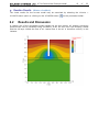
1
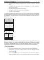
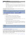
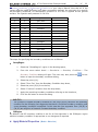
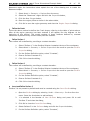
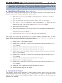
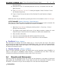
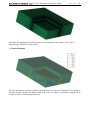
2D / 3D AirFlow Modeling Software
Tutorial Manual
Written by:
Robert Thode, B.Sc.G.E.
Edited by:
Murray Fredlund, Ph.D., P.Eng.
SoilVision Systems Ltd.
Saskatoon, Saskatchewan, Canada
Software License
The software described in this manual is furnished under a license agreement. The software may be used or
copied only in accordance with the terms of the agreement.
Software Support
Support for the software is furnished under the terms of a support agreement.
Copyright
Information contained within this Tutorial M anual is copyrighted and all rights are reserved by SoilVision
Systems Ltd. The SVAIRFLOW software is a proprietary product and trade secret of SoilVision Systems.
The Tutorial M anual may be reproduced or copied in whole or in part by the software licensee for use
with running the software. The Tutorial M anual may not be reproduced or copied in any form or by any
means for the purpose of selling the copies.
Disclaimer of Warranty
SoilVision Systems Ltd. reserves the right to make periodic modifications of this product without obligation
to notify any person of such revision. SoilVision does not guarantee, warrant, or make any representation
regarding the use of, or the results of, the programs in terms of correctness, accuracy, reliability, currentness,
or otherwise; the user is expected to make the final evaluation in the context of his (her) own problems.
Trademarks
Windows™ is a registered trademark of M icrosoft Corporation.
SoilVision® is a registered trademark of SoilVision Systems Ltd.
SVOFFICE ™ is a trademark of SoilVision Systems Ltd.
SVFLUX ™ is a trademark of SoilVision Systems Ltd.
CHEM FLUX ™ is a trademark of SoilVision Systems Ltd.
SVAIRFLOW ™ is a trademark of SoilVision Systems Ltd.
SVHEAT ™ is a trademark of SoilVision Systems Ltd.
SVSOLID ™ is a trademark of SoilVision Systems Ltd.
SVSLOPE ® is a registered trademark of SoilVision Systems Ltd.
ACUM ESH ™ is a trademark of SoilVision Systems Ltd.
FlexPDE® is a registered trademark of PDE Solutions Inc.
Copyright © 2013
by
SoilVision Systems Ltd.
Saskatoon, Saskatchewan, Canada
ALL RIGHTS RESERVED
Printed in Canada
Last Updated: May 20, 2013
Table of C ontents
1 Introduction
3
of
22
............................................................................................................................ 4
2 A Two-Dimensional Example
............................................................................................................................
Model
5
2 .1 M odel Setup
............................................................................................................................ 5
2 .2 Results a nd Discussion
............................................................................................................................ 1 2
3 A Three-Dimensional............................................................................................................................
Example Model
13
3 .1 M odel Setup
............................................................................................................................ 1 3
3 .2 Results a nd Discussion
............................................................................................................................ 2 0
4 References
............................................................................................................................ 22
Introduction
1
4
of
22
Introduction
The Tutorial Manual serves a special role in guiding the first time users of the SVAIRFLOW
software through a typical example problem. The example is "typical" in the sense that it is
not too rigorous on one hand and not too simple on the other hand.
The Tutorial Manual serves as a guide by: i) assisting the user with the input of data
necessary to solve the boundary value problem, ii) explaining the relevance of the solution
from an engineering standpoint, and iii) assisting with the visualization of the computer
output. An attempt has been made to ascertain and respond to questions most likely to be
asked by first time users of SVAIRFLOW.
It should be noted that some models presented in this manual can be run with the free
STUDENT authorization of the software. Other models require a purchased STANDARD, or
PROFESSIONAL authorization level to run through the tutorial. The authorization level
required for each model is specified at the start of the model.
A Two-Dimensional Example Model
2
5
of
22
A Two-Dimensional Example Model
The following example will introduce some of the features included in SVAIRFLOW and will
set up a model of a simple air injection well. The purpose of this model is to determine the
effects of a silt layer on the air pressure contours around an injection well. The well
dimensions have been exaggerated for simplicity and viewing purposes. The model
dimensions and material properties are provided below.
Project:
USMEP_Textbook
Model:
SingleWellwSilt
Minimum authorization required: STUDENT
Model Description and Geometry
Material Properties
Sand: air conductivity, ka = 2.18E-04 m/s
Silt: air conductivity, ka = 2.18E-05 m/s
2.1
Model Setup
In order to set up the model described in the preceding section, the following steps will be
required. The steps fall under the general categories of:
a.
C reate model
b.
Enter geometry
A Two-Dimensional Example Model
c.
Specify boundary conditions
d.
Apply material properties
e.
Specify model output
f.
Run model
g.
Visualize results
6
of
22
a. Create Model
The following steps are required to create the model:
1.
Open the SV O FFIC E M a na g e r dialog,
2.
Press the C lear Search button (if enabled),
3.
C reate a new project called UserTutorial by pressing the Ne w button next to the
list of projects. If the project is already present select it,
4.
C reate a new model called User_SingleWellwSilt by pressing the Ne w button
next to the list of models,
5.
Select the following:
Application:
SVAIRFLOW
System:
2D Vertical
Type:
Steady-State
Units:
Metric
Time Units:
Seconds (s)
7.
C lick on the W o rld C o o rd ina te Sy s te m tab on the C re a te Ne w M o d e l dialog,
8.
Enter the World C oordinates System coordinates shown below into the dialog,
9.
x - minimum: -5
x - maximum:
55
y - minimum: -5
y - maximum:
55
C lick O K to close the dialog.
The workspace grid spacing needs to be set to aid in defining region shapes. The
SandyRegion region of the model has coordinates of a precision of 0.5m. In order to
effectively draw geometry with this precision using the mouse, the grid spacing must be set
to a maximum of 0.5.
1.
The O p tio ns dialog will appear. Enter 0.5 for both the Horizontal and Vertical
spacing, under the G rid Sp a c ing tab,
2.
C lick O K to close the dialog.
b. Enter Geometry (Model > Geometry)
Model geometry is defined as a set of regions. Geometry can be either drawn by the user or
defined as a set of coordinates. Model Geometry can also be imported from either .DXF
files or from existing models.
Each region will have separate material properties. To add the necessary region points
follow these steps:
A Two-Dimensional Example Model
1.
7
of
22
Open the R e g io ns dialog by selecting M o d e l > G e o m e try > R e g io ns ... from the
menu,
2.
C hange the first region name from R1 to SandyRegion. To do this, highlight R1
and type the new text,
3.
Press the Ne w button to add a second region,
4.
C hange the name of the second region to SiltRegion,
5.
C lick O K to close the dialog.
The shapes that define each material region will now be created. Note that when drawing
geometry shapes, the region that is current in the region selector is the region the geometry
will be added to. The Region Selector is at the top of the workspace. Enter the geometry as
given below.
Region: SandyRegion
X
Y
0
0
50
0
50
50
26
50
26
35
26
30
24
30
24
35
24
50
0
50
Region: SiltRegion
X
Y
0
28
50
28
50
26
0
26
Geometry in the SVOFFIC E software may be i) typed in manually, ii) cut and pasted from
Excel or directly from the tutorial manual, iii) imported from AutoC AD, or iv) drawn
graphically using the C AD window. In this example we will provide instruments for drawing
the geometry using the C AD window. Prior to drawing geometry shapes it is good to ensure
that snapping is turned on by clicking the "Snap On" at the bottom of the drawing space.
Define the SandyRegion
1.
Ensure the SandyRegion region is current in the region selector drop-down,
2.
Select Dra w > G e o m e try > R e g io n P o ly g o n... from the menu or press the
3.
Move the cursor near (0,0) in the drawing space and left-click the button to
to o lb a r button,
initiate drawing the shape. You can view the coordinates of the current position
A Two-Dimensional Example Model
8
of
22
the mouse is at in the status bar just below the drawing space,
4.
Now move the cursor to subsequent points on the region, clicking once on each
region point,
5.
For the last point, move the cursor near the point (0,50) and double-click on the
point to finish the shape. A line is now drawn from (24,50) to (0,50) and the
shape is automatically finished by SVAIRFLOW by drawing a line from (0,50)
back to the start point, (0,0),
If the SandyRegion geometry has been entered correctly the shape should look like the
model diagram at the beginning of this tutorial.
NO TE:
If a mistake was made entering the coordinate points for a shape, edit the shape using
the R e g io n P ro p e rtie s dialog (menu item M o d e l > G e o m e try > R e g io n P ro p e rtie s ...).
Please also see the following sections in the user's manual to undo changes, move a
point, move multiple points, delete points, or subdivide a line segment.
Define the SiltRegion
6.
Ensure that SiltRegion is current in the region selector,
7.
Select Dra w > G e o m e try > R e g io n P o ly g o n... from the menu,
8.
Move the cursor near (0,28) in the drawing space and left click,
9.
To select the point as part of the shape left click on the point,
10. Now move the cursor near (50,28) and left click on the point. A line is now
drawn from (0,28) to (50,28),
11. Repeat the process for the rest of the points in the region,
12. For the final point, move the cursor near the point (0,26) and double-click on
the point to finish the shape. A line is now drawn from (50,26) to (0,26) and the
shape is automatically finished by SVAIRFLOW by drawing a line from (0,26)
back to the start point, (0,0).
NO TE:
At times it may be tricky to snap to a grid point that is near a line defined for a region.
Turn the object snap off by clicking on "OSNAP" in the status bar to alleviate this
problem.
c. Specify Boundary Conditions (Model > Boundaries)
Boundary conditions must be applied to region points. Once a boundary condition is applied
to a boundary point the starting point is defined for that particular boundary condition. The
boundary condition will then extend over subsequent line segments around the edge of the
region in the direction in which the region shape was originally entered. Boundary conditions
remain in effect around a shape until re-defined. The user cannot define two different
boundary conditions over the same line segment.
More information on boundary conditions can be found in M e nu Sy s te m > M o d e l M e nu >
A Two-Dimensional Example Model
9
of
22
B o und a ry C o nd itio ns > 2D B o und a ry C o nd itio ns in your User's Manual. Now that all of the
regions and the model geometry have been successfully defined, the next step is to specify
the boundary conditions. An atmospheric pressure of 101 kPa is applied at the ground
surface. The injection well pressure is 121 kPa.
X
Y
Boundary Condition
0
0
Zero Flux
50
0
C ontinue
50
26
C ontinue
50
28
C ontinue
50
50
Pressure C onstant
26
50
Zero Flux
26
35
Pressure C onstant
26
30
C ontinue
24
30
C ontinue
24
35
Zero Flux
24
50
Pressure C onstant
0
50
Zero Flux
0
28
C ontinue
0
26
C ontinue
Constant
101
121
101
The steps for specifying the boundary conditions are as follows:
SandyRegion
1.
Select the "SandyRegion" region in the drawing space,
2.
From the menu select M o d e l > B o und a rie s > B o und a ry C o nd itio ns .... The
B o und a ry C o nd itio ns dialog will open. The user may also press the
to o lb a r
button to open the boundary conditions dialog,
3.
Select the point (0,0),
4.
Select "Zero Flux" from the Boundary C ondition drop-down,
5.
Select the point (50,0) from the list,
6.
Select "C ontinue" condition from the drop-down,
7.
Apply the remaining boundary conditions referring to the list above,
8.
C lick the O K button to close the dialog.
NO TE:
The Pressure C onstant boundary condition for the point (26,35) becomes the boundary
condition for the following line segments that have a C ontinue boundary condition until
a new boundary condition is specified. In this case the line segments from (26,35) to
(24,30) are all given a Pressure C onstant boundary condition.
SiltRegion
By default a No BC boundary condition is set for all line segments in the SiltRegion region
and this boundary condition is appropriate so no changes are required.
d. Apply Material Properties (Model > Materials)
A Two-Dimensional Example Model
10
of
22
The next step in defining the model is to enter the material properties for the two materials
that will be used in the model. A sand is defined for the majority of the model and a silt layer
extends horizontally through the middle. This section will provide instructions on creating the
sand material. Repeat the process to add the silt material.
1.
Open the M a te ria ls dialog by selecting M o d e l > M a te ria ls > M a na g e r... from the
menu,
2.
C lick the Ne w button to create a new material,
3.
Enter "Sand" for the material name in the dialog which appears,
4.
Press O K and the M a te ria l P ro p e rtie s dialog will open automatically,
NO TE:
When a new material is created, you can specify the display color of the material using
the Fill C olor box on the Material Properties menu. Any region that has a material
assigned to it will display that material's fill color.
5.
Under the C o nd uc tiv ity tab, select the " C onstant" air conductivity option from
6.
Enter the k a value of 2.18E-04 m/s,
7.
C lick O K to close,
8.
Repeat these steps to create the silt material; refer to the data provided in the A
the drop-down,
Two Dimensional Example Model section at the beginning of this tutorial,
9.
Press O K to close the M a te ria ls M a na g e r dialog,
10. Open the R e g io ns dialog by selecting M o d e l > G e o m e try > R e g io ns from the
menu,
11. Select the "Sand" for the SandyRegion using the material drop-down,
12. Select the "Silt" for the SiltRegion using the material drop-down,
13. Press the O K button to accept the changes and close the R e g io ns dialog.
e. Specify Model Output
Two levels of output may be specified: i) output (graphs, contour plots, fluxes, etc.) which
are displayed during model solution, and ii) output which is written to a standard finite
element file for viewing with AC UMESH software. Output is specified in the following two
dialogs in the software:
i) Plot Manager:
ii) Output Manager:
Output displayed during model solution.
Standard finite element files written out for visualization
AC UMESH or for inputting to other finite element packages.
in
PLOT MANAGER (Model > Reporting > Plot Manager)
The P lo t M a na g e r dialog is first opened to display appropriate solver graphs. Boundary
Flux specifications are used to report the rate of flow across a boundary for a steady
state analysis and the rate and volume of flow moving across a boundary in a transient
analysis. Boundary Names must be assigned using the R e g io n P ro p e rtie s dialog and then
Reports selected using the B o und a ry Flux dialog.
A Two-Dimensional Example Model
11
of
22
1.
C lick on the SandyRegion region shape in the workspace with the mouse,
2.
Select M o d e l > B o und a rie s > B o und a ry C o nd itio ns ... from the menu to open the
B o und a ry C o nd itio ns dialog. By default the point (0,0) has a Boundary Name
defined,
3.
Select the point (26,35),
4.
Enter the boundary name "WellScreen" in the Boundary Name textbox,
5.
Select point (24,35) from the list,
6.
Enter "End" as the boundary name,
7.
Press O K to close the dialog.
Once the Boundary Names have been defined, the plots can be defined.
1.
Select M o d e l > R e p o rting > P lo t M a na g e r... from the menu to open the P lo t
M a na g e r dialog,
2.
Select the B o und a ry Flux tab and press the R e p o rt button found in the Add New
Plot groupbox,
3.
Select "WellScreen" as the boundary and enter WellScreen as the title,
4.
Select the O utp ut O p tio ns tab and click the Display and Save PG6 solver option,
5.
Press O K to return to the P lo t M a na g e r dialog,
6.
C lick O K to close the P lo t M a na g e r dialog and return to the workspace.
There are many plot types that can be specified to visualize the results of the model. A few
will be generated for this tutorial example model including a plot of the solution mesh, air
pressure contours, and flux vectors. These plots may be automatically generated by
pressing the A d d De fa ults button.
f. Run Model
(Solve > Analyze)
The next step is to analyze the model. Select So lv e > A na ly ze from the menu. This action
will write the descriptor file and open the FlexPDE solver. The solver will automatically begin
solving the model.
A Two-Dimensional Example Model
12
of
22
g. Visualize Results (Window > AcuMesh)
The visual results for the current model may be examined by selecting the W ind o w >
A C U M ESH menu option or clicking on the A C U M ESH button
2.2
on the processes toolbar.
Results and Discussion
A contour plot of the completed model results can be seen below. All outputs previously
specified can now be visualized using AC UMESH. It can be seen from the following results
that the silt layer inhibits the flow of air. Lateral flow in the air is therefore unlikely in this
instance.
A Three-Dimensional Example Model
3
13
of
22
A Three-Dimensional Example Model
The following example will introduce you to the three-dimensional SVAIRFLOW modeling
environment. The purpose of this model is to calculate the quantity of air-flow into the
basement. A 1 cm crack exists between the floor slab and the basement walls. The intent of
the current model is to calculate the volume of contaminated air which will enter the
basement in these specific conditions.
Project:
Foundations
Model:
FloorLeak
Minimum authorization required: STANDARD
Model Description and Geometry
3.1
Model Setup
In order to set up the model described in the preceding section, the following steps will be
required. The steps fall under the general categories of:
a.
C reate model
b.
Enter geometry
c.
Specify initial conditions
d.
Specify boundary conditions
A Three-Dimensional Example Model
e.
Apply material properties
f.
Specify model output
g.
Run model
h.
Visualize results
14
of
22
a. Create Model
Since FULL authorization is required for this tutorial, the user must perform the following
steps to ensure full authorization is activated:
1.
Plug in the USB security key,
2.
Go to the File > A utho riza tio n dialog on the SVOFFIC E Manager,
3.
Software should display full authorization. If not, it means that the security
codes provided by SoilVision Systems at the time of purchase have not yet
been entered. Please see the Authorization section of the SVOFFIC E User's
Manual for instructions on entering these codes.
The following steps are required to create the model:
1.
Open the SV O FFIC E M a na g e r dialog,
2.
Select the project called UserTutorial by pressing the Ne w button next to the list
of projects,
3.
C reate a new model called UserFloorLeak by pressing the Ne w button next to
the list of models. The new model will be automatically added under the recently
created UserTutorial project. The first step in defining the model is to specify the
settings that will be used for the model. To open the Se tting s dialog select M o d e l
> Se tting s in the workspace menu. Select the following settings:
Application:
SVAIRFLOW
System:
3D Vertical
Type:
Steady-State
Units:
Metric
Time Units:
Seconds (s)
4.
Access the W o rld C o o rd ina te Sy s te m tab on the C re a te Ne w M o d e l dialog,
5.
Enter the World C oordinates System coordinates shown below into the dialog,
6.
x - minimum: 45
x - maximum:
75
y - minimum:45
y - maximum:
75
C lick O K to close the dialog.
b. Enter Geometry (Model > Geometry)
Model geometry is defined as a set of regions and a series of layers. Geometry can be either
drawn by the user or defined as a set of coordinates. Model Geometry can also be
imported from either .DXF files or from existing models.
A Three-Dimensional Example Model
15
of
22
This model will be defined by three regions, which are named Outer, Basement, and C rack.
To add the necessary regions follow these steps:
Open the R e g io ns dialog by selecting M o d e l > G e o m e try > R e g io ns from the
1.
menu,
2.
C hange the first region name from R1 to Outer. To do this, highlight the name
and type new text,
3.
Press the Ne w button to add a second region,
4.
C hange the name of the second region to Basement,
5.
Press the Ne w button to add a third region,
6.
C hange the name of the third region to C rack,
7.
C lick O K to close the dialog.
The shapes that define each region will now be created. Note that when drawing geometry
shapes the region that is current in the region selector is the region the geometry will be
added to. The Region Selector is at the top of the workspace.
Outer
X
50
70
70
50
Basement
Y
50
50
70
70
X
50
59.8
59.8
50
Y
50
50
59.8
59.8
Crack
X
50
59.7
59.7
50
Y
50
50
59.7
59.7
Define the Outer region
1.
Ensure the Outer region is current in the region selector,
2.
Select Dra w > G e o m e try > P o ly g o n R e g io n from the menu,
3.
Move the cursor near (50,50) in the drawing space,
4.
When the cursor is near the point, click the left mouse button. The cursor should
automatically snap to the point (50,50) as long as the SNAP and GRID options in
the status bar are both bold,
5.
Now move the cursor to subsequent region points and repeat the left-click
procedure,
6.
For the last point (50,70), double-click on the point to finish the shape. A line is
now drawn from (70,70) to (50,70) and the shape is automatically finished by
SVAIRFLOW by drawing a line from (50,70) back to the start point, (50,50).
NO TE:
Select a shape with the mouse and select Ed it > De le te from the menu if a mistake was
made entering the coordinate points for a shape. This will remove the entire shape
from the region. To edit the shape use the R e g io n P ro p e rtie s dialog.
Define the Basement
In the instructions for defining the Outer shape the command line was used. To draw the
A Three-Dimensional Example Model
16
of
22
Basement region the instructions below explain the use of the drawing tool to create the
Basement shape.
7.
Select M o d e l > G e o m e try > R e g io ns from the menu,
8.
Select the "Basement" region and click the P ro p e rtie s button,
9.
C lick the Ne w P o ly g o n button,
10. Enter the region points as shown in the above table,
11. C lick O K to save the region geometry and close the R e g io n P ro p e rtie s dialog.
Define the Crack
Follow the above method to define the C rack shape, referring to the table of points above.
After all the region geometry has been entered it will appear like the diagram at the
beginning of this tutorial. This model consists of three surfaces defined by constant
elevations. By default every model initially has two surfaces.
Define Surface 1
This surface will be defined by providing a constant elevation.
1.
Select "Surface 1" in the Surface Selector located at the top of the workspace,
2.
Select M o d e l > G e o m e try > Surfa c e P ro p e rtie s in the menu to open the Surfa c e
P ro p e rtie s dialog,
3.
For the Surface Definition option, select "C onstant",
4.
Enter a Surface C onstant of 0,
5.
C lick O K to close the dialog,
Define Surface 2
This surface will be defined by providing a constant elevation.
6.
Select "Surface 2" in the Surface Selector located at the top of the workspace,
7.
Select M o d e l > G e o m e try > Surfa c e P ro p e rtie s in the menu to open the Surfa c e
8.
For the Surface Definition option, select "C onstant",
9.
Enter a Surface C onstant of 4,
P ro p e rtie s dialog,
10. C lick O K to close the dialog.
Insert and Define Surface 3
Surface 3 is not present by default and must be created using the Ins e rt Surfa c e dialog.
1.
Open the Surfa c e s dialog by selecting M o d e l > G e o m e try > Surfa c e s from the
menu. Press the Ne w button to add surfaces,
2.
1 is selected in the Number of Ne w Surfa c e s dialog and press O K to add
"Surface 3" and close the dialog,
3.
C lick O K to close the Ins e rt Surfa c e dialog,
4.
Select Surface 3 in the Surfa c e s dialog and click the P ro p e rtie s button,
5.
For the Surface Definition option, select "C onstant" ,
A Three-Dimensional Example Model
6.
Enter a Surface C onstant of 5.5,
7.
C lick OK to close the dialog.
17
of
22
c. Specify Initial Conditions (Model > Initial Conditions)
A temperature of 20oC is required.
1.
Select M o d e l > Initia l C o nd itio ns > Se tting s from the menu,
2.
Move to the T e m p e ra ture tab,
3.
Select the " C onstant/Expression Temperature" Option,
4.
Enter a temperature value of 20,
5.
C lick O K to close the Se tting s dialog.
d. Specify Boundary Conditions (Model > Boundaries)
More information on boundary conditions can be found in M e nu Sy s te m > M o d e l M e nu >
B o und a ry C o nd itio ns in your User's Manual.
Now that all of the regions, surfaces, and the materials have been successfully defined, the
next step is to specify the boundary conditions on the region shapes. The ground surface will
be set at a pressure of 101.3 kPa while the basement will be set at a pressure of 101.2 kPa.
The steps for specifying the boundary conditions include:
1.
Select the "Outer" region in the drawing space,
2.
Select "Surface 3" in the surface selector,
3.
From the menu select M o d e l >
B o und a rie s
>
B o und a ry
C o nd itio ns. The
b o und a ry c o nd itio ns dialog will open and display the boundary conditions for
Surface 3,
4.
Move to the Surfa c e B o und a ry C o nd itio ns tab,
5.
From the Boundary C ondition drop-down select a Pressure Expression boundary
condition. This will cause the Expression box to be enabled,
6.
In the Expression box enter a pressure of 101.3,
7.
C lick the O K button to save the boundary condition to the list.
Now, to set the C rack regions Surface 2 Boundary C ondition to 101.2 kPa:
1.
Select the "C rack" region in the drawing space,
2.
Select "Surface 2" from the surface drop-down,
3.
From the menu select M o d e l > B o und a rie s > B o und a ry C o nd itio ns ,
4.
C lick the Surfa c e B o und a ry C o nd itio ns tab,
5.
Select the Pressure Expression boundary condition and enter a value of 101.2 in
the expression box,
6.
C lose the dialog using the O K button.
NO TE:
A Three-Dimensional Example Model
18
of
22
The remaining Surfaces are by default set to the None boundary condition, which is
treated as a Zero Flux condition. The remaining Sidewalls are by default set to the No
BC boundary condition, which also is treated as a Zero Flux condition.
e. Apply Material Properties (Model > Materials)
The next step in defining the model is to enter the material property for the material that will
be used in the model. It will be defined for all the regions.
1.
Open the M a te ria ls M a na g e r dialog by selecting M o d e l > M a te ria ls > M a na g e r
from the menu,
2.
C lick the Ne w button to create a material. Enter "Soil1" for the name,
3.
The M a te ria l P ro p e rtie s dialog will open automatically; or, select the new
material and click P ro p e rtie s to open the M a te ria l P ro p e rtie s dialog,
4.
Move to the C o nd uc tiv ity tab,
5.
Enter the k a expression of 7E-08*(z/5.5) m/s . This expression will cause the air
conductivity to vary with depth, z,
6.
Press O K on the M a te ria ls M a na g e r dialog to close both dialogs.
Each region will cut through all the layers in a model creating a separate block on each
layer. Each block can be assigned a soil or be left as void. A void area is essentially air
space. In this model all blocks will be assigned a material.
1.
Select "Outer" in the Region Selector,
2.
Select M o d e l > M a te ria ls > M a te ria l La y e rs from the menu to open the M a te ria l
La y e rs dialog,
3.
Select the "Soil1" material from the drop-down for Layer 1,
4.
Select the "Soil1" material from the drop-down for Layer 2,
5.
Select "Basement" in the Region Selector using the right arrow at the top of the
6.
Select M o d e l > M a te ria ls > M a te ria l La y e rs from the menu to open the M a te ria l
7.
Select the "Soil1" material from the drop-down for Layer 1,
8.
Select "C rack" in the Region Selector,
9.
Select M o d e l > M a te ria ls > M a te ria l La y e rs from the menu to open the M a te ria l
M a te ria l La y e rs dialog,
La y e rs dialog,
La y e rs dialog,
10. Select the " Soil1" material from the drop-down for Layer 1,
11. C lose the dialog using the O K button.
f. Specify Model Output
Two levels of output may be specified: i) output (graphs, contour plots, fluxes, etc.) which
are displayed during model solution, and ii) output which is written to a standard finite
element file for viewing with AC UMESH software. Output is specified in the following two
dialogs in the software:
A Three-Dimensional Example Model
i) Plot Manager:
ii) Output Manager:
19
of
Output displayed during model solution.
Standard finite element files written out for visualization
AC UMESH or for inputting to other finite element packages.
22
in
PLOT MANAGER (Model > Reporting > Plot Manager)
The P lo t M a na g e r dialog is first opened to display appropriate solver graphs. There are
many plot types that can be specified to visualize the results of the model. A few will be
generated for this tutorial example model including a plot of the pressure contours,
solution mesh, and gradient vectors.
1.
Open the P lo t M a na g e r dialog by selecting M o d e l > R e p o rting > P lo t M a na g e r
from the menu,
2.
The toolbar at the bottom left of the dialog contains a button for each plot type.
C lick on the C o nto ur button to begin adding the first contour plot. The P lo t
P ro p e rtie s dialog will open,
3.
Enter the title air pressure.
4.
Select "ua" as the variable to plot from the drop-down,
5.
Move to the P ro je c tio n tab,
6.
Select "Plane Projection" option,
7.
Select Y from the C oordinate Direction drop-down,
8.
Enter 50 in the C oordinate field. This will generate a 2D slice at y = 50m on
which the air pressures will be plotted,
9.
C lick O K to close the dialog and add the plot to the list,
10. Repeat these steps 2 to 9 to create the remaining plots. Note that the Mesh plot
does not require entry of a variable,
11. C lick O K to close the P lo t M a na g e r and return to the workspace,
In order to find out the amount of air flowing into the basement, we must define a
surface flux across the Surface 2 (the basement floor) and restrict it to the BasementIn
region. Follow these steps to define this:
12. Open the P lo t M a na g e r dialog by selecting M o d e l > R e p o rting > P lo t M a na g e r
A Three-Dimensional Example Model
20
of
22
from the menu,
13. Select the Surfa c e Flux tab and press the Sum m a ry P lo t button from the Add
New Plot area,
14. The P lo t P ro p e rtie s - Surfa c e Flux dialog will appear. Select "Surface 2" from
the Surface drop-down,
15. Type in C rack Flow as the name of the Surface Flux and Restrict to Region
Basement.
Additional plots may be defined by pressing the De fa ult P lo ts button on the P lo t M a na g e r.
OUTPUT MANAGER (Model > Reporting > Output Manager)
Two types of output files will be generated for this tutorial example model: a transfer file
of air pressure, and a .dat file to transfer the results to AC UMESH.
1.
Open the O utp ut M a na g e r dialog by selecting M o d e l > R e p o rting > O utp ut
M a na g e r from the menu,
2.
The toolbar at the bottom left corner of the dialog contains a button for each
output file type. Press the SV A irFlo w button to create a new transfer file,
3.
Enter the title uaTransfer,
4.
C lick O K to close the dialog and add the output file to the list,
5.
C lick O K to close the O utp ut M a na g e r and return to the workspace.
g. Run Model (Solve > Analyze)
The next step is to analyze the model. Select So lv e > A na ly ze from the menu. This action
will write the descriptor file and open the SVAIRFLOW solver. The solver will automatically
begin solving the model. When the Regrid Limit message appears click "No" and the solver
will begin generating the plots.
h. Visualize Results (Window - AcuMesh)
Once you have analyzed the model, the output plots can be visualized using AC UMESH. In
order to view plots in AC UMESH, select W ind o w > A C U M ESH from the menu. Plots can
visualized by selecting the desired process under Plots in the menu.
3.2
Results and Discussion
After the model has finished solving, the results will be displayed in the dialog of thumbnail
plots within the SVAIRFLOW solver. These plots can also be examined in details using
AC UMESH. This section will give a brief analysis for each plot that was generated.
Solution Mesh
A Three-Dimensional Example Model
21
of
22
The Mesh plot displays the finite-element mesh generated by the solver. The mesh is
automatically refined in critical areas.
Pressure Contours
The plot indicates a pressure gradient causing flow of air into the basement. The results of
the flux section indicate the steady-state flow of air of 4.80e-7 m3/second, equivalent to
0.0415 m3/day is entering the basement.
References
4
22
of
References
FlexPDE 6.x Reference Manual, 2007. PDE Solutions Inc. Spokane Valley, WA 99206.
22