Download Cabri User Manual - Chartwell

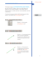
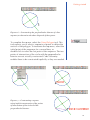
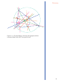
CABRI GEOMETRYTM II Plus
Innovative Math Tools
USER MANUAL
WELCOME!
Welcome to the interactive world of Cabri GeometryTM!
Cabri Geometry was initially designed at IMAG, a joint
research laboratory of CNRS (National Center for Scientific
Reasearch) and Joseph Fourier University in Grenoble, France.
Jean-Marie LABORDE, Cabri’s spiritual father, started the
project in 1985 in order to make it easier to teach and learn
geometry.
Today more than 15 million users enjoy working with
Cabri Geometry, on computers as well as on Texas Instruments
graphing calculators.
Constructing geometrical objects on a computer offers a
whole new dimension compared to doing exercises the
traditional way with pencil, paper, ruler, and compass!
Cabri Geometry II Plus offers a wide range of powerful,
easy-to-use features. You can draw and manipulate plane and
solid figures, from the simplest to the most complex. Freely
manipulate figures at any stage to test the construction, make
conjectures, measure or remove objects, calculate, make
changes, or start all over again. Cabri Geometry II Plus is
cutting-edge tool for teaching and learning geometry,
designed for teachers as well as for students at all levels,
from elementary school to university.
Some features of the program are specific to Macintosh/
Windows versions: Ctrl and Alt keys under Windows
correspond to
option on
z command and to Alt
the Macintosh; a right-click under Windows corresponds to
Ctrl + click on a Mac.
• Interface: New, larger, easy to read icons. More intuitive
pop-up menu for resolving ambiguous selections. Change
the attributes of any object in just a few clicks.
• Labels: Now you can name all graphical objects and
position labels anywhere around an object.
2
• Expressions: Define expressions with one or more
variables and evaluate them dynamically.
• Instantaneous graphs: You can easily draw and study
graphs of one or more functions, and direct manipulation
allows you to explore a function’s results according to its
parameters.
• Loci: Display loci of points or objects, loci of loci, and
intersections with loci. You can also display equations of
algebraic curves drawn using the Locus tool.
• Smart lines: Only the ‟useful” portion of a line is displayed.
You can change the length of that portion as often as you like.
• Colors: Choose objects and text colors as well as the area
fill color from the new extended color palette, or use the
new dynamic color feature.
• Pictures (Bitmaps, JPEG, GIF): Attach any images to objects
in the figure (points, line segments, polygons, background).
The images will be updated during animations and as the
figure is manipulated.
• Text: Edit the style, font, and text attributes of individual
characters.
• Figure Description window: Now you can open a window
to list all stages of the construction (Windows only).
• Recording a session: Record a session as you use the
program. Then display it on-screen or print it at a later date
to monitor students’ progress, and clearly identify any
difficulties they may be experiencing (Windows only).
• Import/Export figures: Figures can be transferred to and
from your computer to Cabri Junior on TI graphing
calculators (TI-83 Plus and TI-84 Plus).
All these unique functions can add new dimensions to your
students’ learning experience.
3
This manual includes two sections:
Part [1] GETTING STARTED - BASIC TUTORIAL is designed for
first time users of Cabri Geometry. It familiarizes them with
Cabri Geometry interface, and provides guidelines on using
the mouse. However, experience shows that people learn
how to use Cabri Geometry very quickly, and that in class,
students are already ‟doing” geometry within half an hour of
using the software.
Part [2] DISCOVERY - INTERMEDIATE TUTORIAL is designed
for new users and suggests activities at the high school level
for discovering the world of interactive geometry.
REFERENCE SECTION.pdf is the complete reference guide for
the software.
MOVING ON - ADVANCED TUTORIAL.pdf suggests more
activities for high school seniors or college undergraduates.
The activities in these documents are to a large extent
independent from one other. Readers are invited to carry out
the detailed construction methods, and then try the listed
exercises.
Cabri Geometry II Plus is hereafter referred to as Cabri Geometry.
Visit our website at www.cabri.com for manual updates and
product news. You will also find links to dozens of
websites and information concerning books about geometry
and Cabri.
The Cabrilog team wishes you many fascinating hours of
constructions, explorations and discovery.
2005 CABRILOG S.A.S.
Cabri Geometry™ is a trademark of CABRILOG S.A.S.
©2005 CABRILOG SAS
Author: Eric Bainville
Translation: Sandra Hoath and Chartwell Yorke
Latest update: June, 30th 2005
For new versions: www.cabri.com
To report errors: [email protected]
Graphic design, page layout & second readings: Cabrilog
4
CONTENTS
GETTING STARTED - BASIC TUTORIAL
CHAPTER
1
P6
PHILOSOPHY
1.1
P6
USER INTERFACE
1.2
P7
USING THE MOUSE
1.3
P9
YOUR FIRST CONSTRUCTION
1.4
P 11
DISCOVERY - INTERMEDIATE
CHAPTER
2
P 16
3
P 23
4
P 27
THE EULER LINE
CHAPTER
HUNT THE POINT
CHAPTER
THE VARIGNON QUADRILATERAL
5
Getting started
CHAPTER
1
GETTING STARTED - BASIC TUTORIAL
PHILOSOPHY
1.1
Cabri Geometry is designed to provide the greatest level of
interaction (mouse, keyboard, etc.), between users and the
software, and in each case to do what users might expect the
software to do: on the one hand by respecting industry
standards, and on the other hand, by following the most
plausible mathematical route.
A Cabri Geometry document consists of a figure which can
be drawn freely anywhere on a virtual 1 meter square sheet
of paper. The figure is built up using standard geometric
objects (points, lines, circles, etc.) and other objects
(numbers, text, formulae, etc.).
A document can also contain construction macros, which
enable intermediate constructions to be memorized and
reproduced, thus extending the program’s functionality.
With Cabri Geometry you can open several documents
simultaneously and cut, copy and paste between them.
6
Getting started
USER INTERFACE
1.2
Title bar
Tool bar
Menu bar
Attributes bar
1
Figure description
Window
Drawing area
Help window
Status bar
The figure above shows the Cabri Geometry main window
and its various sections. When Cabri Geometry is first
loaded, the Attributes toolbar, the Help window and the
Figure Description window are not displayed.
The title bar displays the file name of the figure (when a file
has been opened or saved) or Figure #1,2... if the figure has
not yet been named.
The menu bar lets users manipulate documents, handle
sessions and control the program’s general appearance and
behavior.
Throughout this manual, all commands will be described
as follows: Action from the Menu menu using the format
[Menu]Action. For example, [File]Save As... means Save As...
from the File menu.
The toolbar displays the tools you can use to create and
modify a figure. It consists of several toolboxes, each of
which displays a tool from the toolbox as an icon on the bar.
Single click on a button to choose the corresponding tool.
Click and hold a button to open the toolbox as a drop-down
menu. Drag on another tool to choose that tool; it is then
displayed as the icon for the toolbox.
7
Getting started
Feel free to customize the toolbar, or lock it into a fixed
configuration for classroom use. See chapter [8] PREFERENCES
AND CUSTOMIZATION in the REFERENCE SECTION.pdf.
Properties
Points
Measurement
Lines
Text and symbols
Curves
Attributes
Macros
Transformations
Manipulation
Constructions
In this manual, the Tool command from the Toolbox is
described as [Toolbox]Tool and the corresponding icon is
displayed in the margin. For example, [Lines]Ray represents
the Ray tool from the Lines toolbox. (Some of the labels,
which are too long for the margin, have been abbreviated).
The toolbar icons can be displayed in large or small format. To
change the icon size, move the cursor to the right of the last
tool shown on the toolbar, right-click/Ctrl+click and choose
‟Small Icons”.
The status bar always indicates the active tool (Windows
only).
The attributes bar lets you change the attributes of various
objects: color, style, size... Use the [Options]Show Attributes,
command to display the attributes bar, and [Options]Hide
Attributes to hide it. Alternatively you can use the F9 can
also be used on Windows.
The help window provides outline help for the active tool.
It displays the tool’s anticipated ‟required objects” and what
will be constructed. Press the F1 key to show/hide the help
window.
8
Getting started
The f i g u re d e s c r i p t i o n w i n d ow contains a text
describing the figure. It lists all the constructed objects
and construction methods used. To open this window, use
the [Options]Show Figure Description command, and use
[Options]Hide Figure Description to close it. Or you can
toggle it with the F10 key (Windows only).
Finally, the drawing area shows part of the total area that is
available. Geometrical constructions are carried out in this
drawing area.
USING THE MOUSE
1.3
Most software functions are controlled by the mouse.
• move the mouse to move the cursor
• press a mouse button
• release it
When the mouse is used to move the cursor across the
drawing area, Cabri Geometry informs you of the anticipated
results of a click or a drag-and-drop in three ways:
• the cursor changes shape
• a pop-up message displayed alongside the cursor
• the object being constructed is partially displayed
Depending on the construction, the pop-up message and the
partial object may or may not be displayed.
12
9
Getting started
Here follows a list of the various cursors:
An existing object can be selected.
An existing object can be selected, moved, or used
in a construction.
An existing object has been clicked on in order to
select it, or to use it in a construction.
Several selections are possible for the objects under
the cursor. Click with this cursor to display a menu
for choosing a specific object to be selected from a
pop-up list.
An existing object is being moved.
The cursor is in an unused portion of the sheet, and
a rectangular area can be selected using click-anddrag.
Indicates the pan mode for moving the visible area
of the sheet. To enter this mode at any time, press
and hold down the Ctrl / z key. In this mode,
drag-and-drop slides the worksheet across the
window.
The worksheet is being dragged.
A click will create a new independent, movable
point on the sheet.
A click will create a new point which is either
movable on an existing object, or at the intersection
of two existing objects.
A click will fill the object under the cursor with the
current color.
A click will change the attribute (such as the color,
style, or thickness) of the object under the cursor.
10
Getting started
YOUR FIRST CONSTRUCTION
1.4
To illustrate chapter [1] GETTING STARTED - BASIC TUTORIAL,
we will construct a square, given one of the diagonals.
When you start Cabri Geometry, a new, blank, virtual
drawing sheet is created, and you can immediately start the
construction.
Construct the segment which will be the diagonal of the
square. First choose the [Lines]Segment tool.
Figure 1.1 – Choosing the
[Lines]Segment tool.
Figure 1.2 – Constructing the first
point. A preview of the final
segment moves with the cursor
until the second point has been
created.
Figure 1.3 – The segment is
complete after you create the
second point. The [Lines]
Segment tool remains active,
so you can construct another
segment.
11
Getting started
Now move the cursor across the drawing area: it will take the
following shape . Click once to create the first point.
Continue moving the cursor across the drawing area. A
segment will extend from the first point to the cursor,
showing where the segment will be created. Click to create
the second point. Our drawing now contains two points and
one line segment.
To construct a square, first construct the circle with this segment
as its diameter. The center of the circle is the midpoint
of the segment. To construct this midpoint, choose the
[Constructions]Midpoint tool then move the cursor over the
segment. The pop-up message Midpoint of this segment is
displayed alongside the cursor, whose shape changes to
.
Click to mark the midpoint on the segment.
9
Figure 1.4 – Constructing
the midpoint of a segment.
Select the [Curves]Circle tool and move the cursor near to
the midpoint. The pop-up message This center point is then
displayed. The [Curves]Circle tool requires you to select a
point as the center of the circle, so click on the midpoint to
select it. Then a circle is displayed as you move the cursor.
Move it near to one end of the line segment; the pop-up
message This radius point is displayed. To complete the circle
through the end of the segment, click this point.
12
Getting started
Figure 1.5 – Constructing a circle with the given segment as diameter.
Choose the [Manipulation]Pointer tool to alter the figure. The
only points you can move in the figure are the endpoints of
the line segment and the segment itself. If you move the
cursor over one of those objects, its shape becomes
and
the pop-up message This point or This segment is displayed.
The point or the segment can then be moved by
drag-and-drop and the entire figure is updated automatically:
the segment is redrawn, the midpoint and the circle move
accordingly.
To construct the square, first construct the other diagonal,
which is the diameter of the circle, perpendicular
to the original segment. Construct the perpendicular bisector
of the segment: a line, perpendicular to the segment, through
its midpoint. Select the [Constructions]Perpendicular bisector
tool, and then select the segment by clicking on it.
Cabri Geometry constructs the perpendicular bisector.
13
Getting started
Figure 1.6 – Constructing the perpendicular bisector of a line
segment, to determine the other diagonal of the square.
To complete the square, select the [Lines]Polygon tool. This
tool expects you to select a sequence of points to define the
vertices of the polygon. To terminate the sequence, select the
initial point of the sequence for a second time, or
double-click to select the last point of the sequence. The two
points of intersection of the circle with the perpendicular
bisector are not actually constructed: Cabri Geometry
enables them to be constructed implicitly as they are needed.
Figure 1.7 – Constructing a square
using implicit construction of the points
of intersection of the circle and the
perpendicular bisector.
14
Getting started
In other words, select one endpoint of the segment as the
first vertex of the polygon, then move the cursor to one of
the intersection points of the circle and the perpendicular
bisector. A pop-up message Point at this intersection is
displayed to indicate that a mouse-click will construct the
intersection point and at the same time select it as the next
vertex of the polygon. Click at this location to create this
point, then select the other endpoint of the line segment and
the second intersection point of the perpendicular bisector.
Finally select the initial point of the sequence a second time
(or double-click to select the last point of the polygon).
Figure 1.8 – Your first Cabri Geometry construction!
15
Discovery
CHAPTER
2
THE EULER LINE
In this chapter, we will construct a general triangle ABC,
then its three medians. These are the lines that join a vertex
to the midpoint of the opposite side. Next we construct the
three altitudes of the triangle: the lines through each vertex in
turn, perpendicular to the opposite side. Finally we construct
the three perpendicular bisectors of the sides of the triangle:
lines perpendicular to each side, through the midpoint of the
side. It is a well-known fact that the three altitudes, the three
medians and the three perpendicular bisectors are separately
concurrent, and these points of concurrency lie on a straight
line, called the Euler1 line of the triangle.
To construct a triangle, choose the [Lines]Triangle tool. For
information on how to use the toolbar, see Chapter [1]
GETTING STARTED - BASIC TUTORIAL in the previous
section.
Once the [Lines]Triangle tool is active, click in an empty
space to create three new points in the drawing area. These
points can be labeled on the fly immediately after their
creation simply by typing their name on the keyboard. Once
the triangle has been constructed, you can move these labels
around the points to place them outside the triangle, for
example.
Figure 2.1 – Triangle ABC is constructed using the [Lines]Triangle
tool. The vertices are labeled on the fly by typing their name at the
time they are created.
1
Léonard Euler,
1707-1783
16
Discovery
To move an object’s name, use the [Manipulation]Pointer
tool. Drag the name by positioning the cursor over it until the
pop-up message This label appears, then hold down the
mouse button while dragging the mouse to move the name
to the desired location. To change the name of an object,
choose the [Text and symbols]Label tool and select the name;
an editing window is displayed.
Use the [Constructions]Midpoint tool to construct midpoints.
To construct the midpoint of AB, first select A then B.
Another way to construct the midpoint of a segment is to select
the segment itself. You can name the new point on the fly, say C’.
Construct the midpoints of the other sides the same way: A’ on
BC and B’ on CA.
Figure 2.2 – [Left]. To construct the midpoints, use the
[Constructions]Midpoint tool, which accepts as arguments two
points, a segment, or the side of a polygon.
[Right]. To construct medians, use the [Lines]Line tool and to
change their color using the [Attributes]Color... tool.
The [Manipulation]Pointer tool lets you freely move about the
independent, movable objects of a construction. In this case,
the three points A, B and C are the independent, movable
objects. The entire construction is updated automatically as
soon as any of them is moved. Thus you can explore a variety
of configurations for the construction. To see which objects in a
figure are movable, choose the [Manipulation]Pointer tool, then
click and hold on an empty part of the drawing area. After a
short delay, the movable objects are displayed as marquees (also
known as ‟marching ants”).
17
Discovery
Use the [Lines]Line tool to construct the three medians. For
the line AA’, click successively on A then A’.
Use the [Attributes]Color... tool to change the line color.
Select the color from the palette by clicking on it, and then
click on the object to be colored.
Choose the [Points]Point tool, and then move the pointer
near to the point of intersection of the three medians.
Cabri Geometry tries to create the point of intersection
of two lines but, since there is an ambiguity (there are
three concurrent lines to choose from) a menu appears
so you can select which two lines to use to construct
the intersection point. As you move the cursor down the
list of objects, the corresponding lines in the figure are
highlighted. Label the point of intersection of the medians G.
Figure 2.3 – Constructing the point of intersection of the medians,
and resolving the ambiguities of a selection.
18
Discovery
Use the [Constructions]Perpendicular line tool to construct
the altitudes of the triangle. This tool creates the unique line
which is perpendicular to a given direction, through a given
point. Therefore, select a point and: a line, a segment, a ray,
etc. The order of selection is irrelevant. To construct the
altitude through A, select A then the side BC. Use the same
method to construct the altitudes through B and C. As for the
medians, choose a color for the altitudes, and construct their
point of intersection H.
Use the [Constructions]Perpendicular bisector tool to
construct the perpendicular bisector of a segment. Select the
segment or its two extremities. Label the point of intersection
of the three perpendicular bisectors as O.
Figure 2.4 – [Left]. Constructing altitudes using the
[Constructions]Perpendicular line tool.
[Right]. Constructing the perpendicular bisectors using the
[Constructions]Perpendicular bisector tool.
You can use the [Properties]Collinear? tool to check whether
the three points O, H and G are collinear. By selecting each
of these points in turn, then clicking somewhere on the
drawing area, Cabri Geometry displays whether the points
are collinear.
If you move independent points of the figure, this text is
updated at the same time as the other parts of the figure.
19
Discovery
To construct the Euler line of the triangle through the three
points O, H and G, use the [Lines]Line tool and select, for
example, O and H. Use the [Attributes]Thick... tool to make
this line stand out.
Figure 2.5 – [Left]. Checking the collinearity of the three points O,
H and G. The [Properties]Collinear? tool creates a text message
Points are collinear or Points are not collinear.
[Right]. The Euler line of the triangle, shown clearly by its
increasing thickness with the [Attributes]Thick... tool.
If you change the shape of the triangle by moving the
relative position of the vertices, it is apparent that G is always
between O and H, and also that its relative position on the
line segment does not change. Suppose we check this by
measuring the lengths of GO and GH. Choose the
[Measurement]Distance or length tool. This tool measures the
distance between two points, or the length of a line segment,
depending on the object selected. Select G and then O: the
distance from G to O appears, measured in centimeters. Do
the same for G and H. Once you have taken the
measurement, you can edit the corresponding text message
by adding the characters ‟GO=” in front of the number, for
example (Windows only).
20
Discovery
Figure 2.6 - [Left]. Using the [Measurement]Distance or length
tool to find the lengths of GO and GH.
[Right]. Using the calculator – [Measurement]Calculate... – to
display the ratio GH/GO and show that it is always equal to 2.
By making changes to the original triangle, you can see that
GH is always twice the length of GO. To verify this, we can
calculate the ratio GH/GO. Choose the [Measurement]
Calculate... tool. Select the text message giving the distance
GH, then the operator /, and finally the text message giving
GO. Click on the = key to obtain the result, which can be
dragged and dropped onto the drawing area. If you select a
number ([Manipulation]Pointer tool), you can increase or
decrease the number of digits displayed using the + and
– keys on the keyboard. You can display the ratio with ten
or more digits, to show that it is believable that this ratio is
constant and equal to 2.
Exerc i s e 1 - Add a circumscribed circle to the figure, with
center O, passing through A, B and C, using the [Curves]Circle
tool.
Exerc i s e 2 - Next, add the ‟nine-point circle” for the
triangle. This is the circle whose center is at the midpoint of
OH, and which passes through the midpoints of the sides: A’,
B’ and C’, the foot of each altitude, and the midpoint of each
of the line segments HA, HB and HC.
21
Discovery
Figure 2.7 - The final figure, showing the triangle with its
circumscribed circle and ‟nine-point circle”.
22
Discovery
CHAPTER
3
HUNT THE POINT
The following activity illustrates several ways you can explore
with Cabri Geometry. Starting from three given points A, B, C,
look for any points M such that:
MA + MB + MC = 0
First, construct four points at random positions, using the
[Points]Point tool, label them A, B, C and M.
Cabri Geometry allows you to use vectors . Each vector is
represented by a line segment with an arrow. Now, construct
the vector MA using the [Lines]Vector tool, by selecting
first M, then A. This vector has its origin at M. Use the same
method to construct vectors MB and MC.
Next, construct the resultant vector of MA + MB using the
[Constructions]Vector Sum tool. First click on the two
vectors and then on the origin for the resultant, choosing M
in this example. Label the further extremity of the vector as N.
Finally use the same method to construct the resultant of the
three vectors, with M as its origin. Add MN (which equals MA +
MB ) and MC . Label the further extremity of this vector: P.
23
Discovery
N
P
Figure 3.1 - [Left]. Starting from any three points: A, B, C, and a
further point M, the vectors MA , MB and MC are drawn.
[Right]. Constructing MN = MA + MB , and MP = MA + MB + MC
using the [Constructions]Vector Sum tool.
Now look for the solution to the problem diagrammatically.
To do so, choose the [Manipulation]Pointer tool and move
point M. The resultant of the three vectors is updated
continually as you move M around the drawing area.
You can see that the magnitude and direction of MP depend
on the position of M relative to the points A, B and C. Thus
we can make the following conjectures (among others):
• There is only one position of M for which the resultant of
the three vectors is null: the problem has a unique solution.
The solution point is inside the triangle ABC.
• The quadrilateral MANB is a parallelogram.
• The quadrilateral MCPN is a parallelogram.
• For a zero resultant vector, the vectors MN and MC must
be collinear, and in addition they must have the same
magnitude but opposite direction.
• MP always passes through the same point and this point is
the solution to the problem.
• The position of point P is dependent on M. Based on this
fact, we can define a transformation, which links P to M,
and the solution to the problem is an invariant point under
this transformation.
24
Discovery
Suppose for example that we observed that vectors MN and
MC must have opposite directions.
Another question then arises: for which positions of M are
these two vectors collinear? Move M in such a way that the
two vectors are collinear. Observe that M must lie on a straight
line, and that this line passes through C and the midpoint of AB.
The line is therefore the median of the triangle through C. Since
M is equally dependent on A, B and C, note that M must also lie
on the other two medians, and the required point is therefore the
point of intersection of the three medians.
As a class activity, the students could continue by developing
a construction of the solution point, and proving the
conjecture which resulted from the investigation.
A dynamic construction is a much more convincing
illustration than a static figure drawn on a sheet of paper.
In fact, by simply manipulating the figure, we can check the
conjecture in a large number of cases. A conjecture which
remains valid after a figure has been altered will be correct
in the great majority of cases.
In class, raise the following points (among others) with
students:
• Is a dynamic and visually correct construction, actually
correct?
• Is a correct dynamic construction an answer to the question?
• When can a mathematical argument be considered as a
proof?
• What is missing from a dynamic construction to make it a
proof?
• Must a proof be based on the procedure used to draw the
figure?
25
Discovery
Exerc i s e 3 - Extend the problem to four points, by finding
those points M, such that:
MA + M B + M C + M D = 0
Exerc i s e 4 - List all the ‟paths of exploration” and proofs
needed for the initial problem (three points) which are
available to a high school senior.
Exerc i s e 5 - Investigate and construct the points M which
minimize the sum of the distances to three points:
MA+MB+MC. The solution is the Fermat1 point of triangle
ABC.
1
Pierre Simon de Fermat,
1601-1665
32
26
Discovery
CHAPTER
4
THE VARIGNON QUADRILATERAL
The following activity shows some constructions based on
Varignon’s1 Theorem.
First, construct any quadrilateral ABCD. Choose the
[Lines]Polygon tool, then select four points and label them
on the fly: A, B, C, D. To finish off the polygon, reselect A
after constructing D.
Next, construct the midpoints: P of AB, Q of BC, R of CD and S
of DA using the [Constructions]Midpoint tool.
Finally, construct the quadrilateral PQRS, using the
[Lines]Polygon tool.
By altering the figure, using the [Manipulation]Pointer tool,
you can see that PQRS always seems to be a parallelogram.
You can use the [Properties]Parallel? tool to have
Cabri Geometry determine whether the lines PQ and RS are
parallel, then do the same for PS and QR. To do this , first
select the side PQ and then RS: a text message will appear,
confirming that the two sides are indeed parallel. Use the
same method to check that PS and QR are parallel.
1
Pierre Varignon,
1654-1722
27
Discovery
Figure 4.1 - [Left]. Starting from any quadrilateral ABCD,
construct the quadrilateral PQRS with vertices at the midpoints
of the sides of ABCD.
[Right]. Construction the diagonals of PQRS, and the demonstration
that they bisect each other.
Now we will construct the two diagonals PR and QS, using
the [Lines]Segment tool, and their point of intersection I
using the [Points]Point tool. There are several ways to
demonstrate that I is the midpoint of both PR and QS, and
that therefore PQRS is a parallelogram. For example, you
can use centers of mass: P can be considered as the center of
mass of two particles of equal mass at A and B{(A,1),(B,1)}.
Similarly R is the center of mass of particles of equal mass at
C and D{(C,1),(D,1)}. Thus the midpoint of PR is the center
of mass of {(A,1),(B,1),(C,1),(D,1)}. The midpoint of QS is the
same thing. Hence the two midpoints coincide: at the point
of intersection I.
Var i g n o n ’s Th e o re m . The quadrilateral PQRS whose
vertices are the midpoints of the sides of any quadrilateral
ABCD, is a parallelogram whose area is half that of ABCD.
Exe r c i s e 6 - Now show that the second part of the theorem
concerning the area of PQRS is true. Hint: use the figure
shown in Figure 4.2.
28
Discovery
Figure 4.2 - The construction
for demonstrating the second
part of the theorem.
Without modifying A, B and C, move D so that PQRS
appears to be a rectangle. Since we already know that PQRS
is a parallelogram, it is sufficient to show that one of its
angles is a right angle. Therefore measure the angle at P,
using the [Measurement]Angle tool. This tool expects you
to select three points, where the second point is the vertex
of the angle. Here, for example, you should select S, P (the
vertex of the angle) and Q.
Figure 4.3 - Measuring angle P
of parallelogram PQRS.
You can also use the [Measurement]Angle tool to determine
the size of an angle which has previously been marked
with the [Text and symbols]Mark Angle tool. You must also
select three points for this tool, in the same order as for
[Measurement]Angle. By moving D so that PQRS is a
rectangle,you can see that there are an infinite number of
solutions, as long as D lies on one straight line. In fact, if you
draw the diagonals AC and BD of the quadrilateral ABCD,
you can see that the sides of PQRS are parallel to them,
and hence PQRS is a rectangle if and only if AC and BD are
perpendicular. To ensure that PQRS is always a rectangle, we
need to redefine the position of D. Draw the line AC with the
[Line]Line tool by selecting A and C, then draw the
perpendicular to this line which passes through B, using the
[Constructions]Perpendicular line tool, selecting B and the
line AC.
29
Discovery
D is currently an independent, movable point of the figure.
Modify this so that it becomes a point which is constrained
to lie on the perpendicular to AC passing through B. Choose
the [Constructions]Redefine Object, then select D. A menu
appears listing the various options for redefining D. Choose
Point on object, then select any point on the perpendicular.
D moves to this point, and thereafter is constrained to be on
the designated line.
Redefinition is a powerful investigative tool. It allows you to
increase or decrease the number of degrees of freedom of the
parts of a figure without having to redraw it from scratch.
Figure 4.4 - Point D is now redefined so that PQRS is always a
rectangle. D still has one degree of freedom, being able to move
along a line.
Exer c i s e 7 - Find a necessary and sufficient condition that
PQRS is a square. Redefine D again, so that the construction
will only produce squares.
Figure 4.5 - Here, D has no degrees of freedom at all and PQRS
is always a square.
30