Download Introduction to Lab Instruments

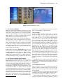
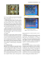
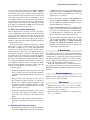
ECE316, Experiment 00, 2015
Communications Lab, University of Toronto
Introduction to Lab Instruments
Bruno Korst - [email protected]
Abstract
This experiment will review the use of three lab instruments as well the time domain and frequency domain
characteristics of two common types of signals. The experiment will guide the students through exercises in
order to create a foundation for the rest of the course.
Keywords
Oscilloscope — Signal Generator — Impedance — Decibel
Contents
1. Suggested Reading
Introduction
1
1
Suggested Reading
1
2
The Instruments
1
2.1 The Tektronix AFG3021 . . . . . . . . . . . . . . . . . . 2
2.2 The Tektronix TDS 2012 Oscilloscope . . . . . . . . 2
The Trigger • The Math/FFT Function • Cursors • The Measure
Feature • The Scan Mode
2.3 Spectrum Analyzer . . . . . . . . . . . . . . . . . . . . . 4
3
Exercises
4
3.1 With a Sine Wave and the Oscilloscope . . . . . . . 4
3.2 With a Pulse and the Oscilloscope . . . . . . . . . . 5
3.3 With FM and the Spectrum Analyzer . . . . . . . . . 5
4
Conclusion
5
Acknowledgments
5
References
5
You, as a learner, will benefit most from the practice in this
lab by avoiding the automatic settings of the instruments. You,
as an Engineer, must understand what you need from the
instrument prior to letting the instrument choose it for you.
This is to say that you will benefit from learning how to set
the instrument first (this should take about three experiments)
and only then go for the automatic features. If you can explain
what the automatic features do, go ahead and use them.
There is no standard background reading to prepare you
to use the instruments. Your best option is to explore the instruments either during the experiments or at the laboratory in
your free time. A good reference is [1], in particular the second half of the book, which is dedicated to explaining some of
the instruments found in a teaching lab. The websites for manufacturers such as Agilent and Tektronix do offer literature
about their instruments, which may be helpful. Manuals for
the instruments [2] [3] are available both at the manufacturer’s
website and at the lab.
Introduction
This first experiment is a review of very basic concepts in
Electrical Engineering, done with the help of common instruments found in a lab. In the process, you will review some
features of the instruments that will be useful in all courses
in Communications and Digital Signal Processing. In most
experiments, you will simulate a system, implement it on hardware and test it with actual signals and instruments. Though
this experiment appears to be rudimentary, what you practice
here will be used in all future experiments.
You will review the time domain and frequency domain
representation through the use of sinusoids and pulses. You
will be guided to perform some exercises with the three types
of basic instruments:
• An Arbitrary Signal Generator;
• An Oscilloscope;
• A Spectrum Analyzer.
2. The Instruments
Since you will implement your systems on a DSP platform, all
your input signals from the signal generator will be presented
to an analog-to-digital converter prior to being processed by
the DSP. The input of the converter is a high-impedance input.
By default, your signal generator assumes a 50Ω impedance
at their output. This is to say that you must adjust the output
of the signal generators to “see” a large impedance. This is
done by choosing a High Z output option, as described below.
In a similar fashion, the input to the oscilloscope – as a
measuring device – is a very high impedance input. This is
so to prevent the instrument itself from interfering with the
measurement being taken. The instrument must look like an
open circuit to the device under test. The very high (around
1MΩ) input impedance will accomplish this. There is no
setting to be changed on the oscilloscope.
Introduction to Lab Instruments — 2/5
(a) Finding Output Menu (Output ON)
(b) Selecting High Z
Figure 1. Tektronix AFG 3021 - Output
2.1 The Tektronix AFG3021
In this lab you will use the Tektronix AFG3021. It is called
arbitrary because it allows for waveforms to be designed and
edited either on the instrument or on a computer, and then
loaded onto the instrument. Some of your experiments will
utilize arbitrary (i.e., made up) waveforms. Below are two
settings which you will need throughout the course.
Turn the instrument on 1 . From the front panel, press
Sine. You will see on the bottom right corner of your screen
a menu labeled Output Menu. Press on the corresponding
button. Another menu will appear, in which you will find
Load Impedance. Press on it, and you will have three options.
Select High Z. From this point on, your instrument is set to
see a high impedance load on its output. To return to the main
screen, just press on Sine again.
Action
Make sure that the Output ON button is lit (if it
is not, press it). It is located right above the BNC output
connector. Otherwise you will not have a signal. Note that
the Output ON button is lit on Figure 1(a). When the output
is ON, and the output impedance is set to high, the message
Load High Z will appear on the top right corner of the screen.
Action
2.2 The Tektronix TDS 2012 Oscilloscope
You may already be familiar with the oscilloscope (every
Electrical Engineer should!), but it is good to review some
features that if not understood now will potentially cause you
to waste precious time during the experiments. These are:
the trigger, the MATH/FFT function and the use of cursors
for measuring voltage, time, amplitude and frequency. Just
as a reminder, whenever you are in the lab, try very hard
to avoid pressing the Auto Set button. Yes, it is convenient
and very popular, but you will not learn as much about the
instrument if you always use it. Students tend to assume that
whatever is displayed after this button is pressed must be the
truth. Always read the numbers and see if they make sense.
The trick is to know what to expect from the instrument. The
1
it happens
general rule is: if you understand what the Auto Set button
does to get the readings, go ahead and use it.
2.2.1 The Trigger
In general, when you connect a signal source to your oscilloscope the signal ”runs” across your screen. In order for
you to take a reading, you should make it stop. The proper
way to make it stop is to set up a voltage level at which the
oscilloscope starts to collect and display the signal. In other
words, you should set up a trigger point. This is done by
pressing the Trig Menu button found at the right-most portion
of your front panel, right under a rotating knob. As you press
it, a soft menu appears on the right side of the display. Select
the trigger Source (i.e. channel 1 or 2 – we will not use any
other), and a small arrow will appear further to the right of the
display. The colour of the arrow is the same as the channel
chosen as the source. This arrow indicates your trigger level.
Rotate the knob that is over the Trig Menu button, and the
arrow will move. Position the arrow within the voltage span
of your signal. This will make the signal stop on the display.
Note that the signal continues to be collected and displayed,
but it is now steady on your display. If the signal changes in
amplitude, frequency, or a feature appears, the display will
show it.
The improper way to make a signal stop is to press the
Run/Stop button. In the exercise section of this document you
will do an exercise to understand why using Run/Stop will not
be appropriate.
2.2.2 The Math/FFT Function
This scope allows you to see your signal in the frequency
domain by means of an FFT operation. You can select the
Math mode by pressing a big fat red button right in the middle
of the instrument.
Figure 3 below shows you the time domain for two input
channels and the corresponding frequency domain for one of
those channels. Both inputs are a 1KHz, 1Vpp sine wave.
After pressing the Math Menu button, you must select
what type of operation you want the instrument to perform.
Introduction to Lab Instruments — 3/5
Figure 2. Big Fat Red Button – Math Mode
(a) Time Domain: Two channels
For the case of an FFT, you also must select the channel
(Source) that you want to display. Figure 3(b) is showing the
FFT mode for Channel 1.
On FFT mode, the horizontal control works “opposite”
to its time domain operation. This is to say that if you want
to ”increase” the Hertz per Division reading you should turn
the horizontal scale knob clockwise. In this case, what the
instrument is actually doing is selecting a different sampling
rate for the input at every click of the horizontal scale knob.
You should be careful when using this knob to zoom in, as you
may end up with aliasing depending on the type of signal you
have (this will likely happen in the exercise section below).
The proper way to zoom into the signal in the frequency
domain is to use the FFT Zoom soft key. Note also that as you
turn the horizontal scale knob, at the bottom of the screen the
number displayed changes, as it represents the horizontal scale
units of Hz per Division. Figure 3(b) shows the frequency
component at 1KHz.
2.2.3 Cursors
In order for you to perform specific or relative measurements
between points of a signal, the instrument allows you to place
cursors on the desired points, and presents you with the values
at each cursor and the calculation for the difference between
the cursors. Cursors can measure differences in time (vertical
cursors) and amplitude (horizontal cursors), or in Math mode
they can measure differences in magnitude and frequency.
After pressing the cursors button on the top part of the front
panel, you will be presented with a menu to select the signal
source (Channel 1, 2 or math) and the type of measurement
you want.
2.2.4 The Measure Feature
The Measure button is found on the top part of the front panel.
This feature is very convenient, but you should try to develop
an intuition whether the numbers displayed make sense. This
usually comes with practice. For instance, if your measured
output from the DSP board is a 20 Vpp sine wave, it should
be obvious that this makes absolutely no sense. The power
supply feeds the board with only 12 VDC , and the output of
the codec cannot handle signals greater than 2.7 Vpp . In that
case, consider that maybe your 10x probe option is on! If you
have a rough idea of what to expect, you will question the
(b) Frequency Domain: One Channel
Figure 3. Tektronix TDS 2012 Oscilloscope
displayed value right away. Again, knowing what to expect is
very important.
To use the feature, press on the Measure button. A soft
menu will appear on the right area of the display. You must
select the Source of the measurement (i.e., channel 1, 2 or
Math), and the type of measurement (Vpp , Vrms , frequency,
etc.) When you select it, the measurement will also appear
on the right side of the display. Keep in mind that if the 10x,
100x or 1000x probe factor is set, then the measurement will
be scaled by it. To disable it, you must go to the channel menu
(CH1 Menu, for instance) and disable the probe factor.
2.2.5 The Scan Mode
The scan mode can be a blessing or a curse. It is usually a
curse when you fall into this mode ”by accident”. Such accident happens when your trigger mode is set to Auto (which is
the default value), and you inadvertently turn your horizontal
sweep knob (fast, without noticing) to less than 100ms per
division. When this happens, your display will change very
slowly, and it will take you a couple of seconds to visualize a
full display of your signal. Then you will search every button
on the machine for a way to get out of it (and will not find it!).
The way to get out of it is to turn the horizontal sweep knob
back into something greater than 100ms per division.
Introduction to Lab Instruments — 4/5
But the scan mode can, however, be a blessing if you want
to observe sudden changes that happen in your input. By
using the scan mode, your display will show the signal very
slowly and you will be able to observe changes that would
be imperceptible if it were running in normal mode. In the
exercise section (below) you will play with this mode a little.
2.3 Spectrum Analyzer
The spectrum analyzers found in the Communications Lab are
a standard model which for many years has been used in the
industry: the HP8590L. Rather than detailing the capabilities
of the instrument, you will go through an exercise to facilitate
your practical understanding of it. There are some copies of
the manual in the lab, so feel free to refer to it as well if you
need to explore further.
In general, there are three basic buttons and a main rotating
knob in spectrum analyzers. The buttons are labelled:
• Frequency;
oscilloscope (if you want a sine wave and you see a square
wave, something is wrong).
3.1 With a Sine Wave and the Oscilloscope
Set your signal generator to output a 1Vpp , 1KHz sine wave,
and connect its output to the inputs of the oscilloscope using
a T connector and BNC-to-BNC coaxial cables. On your
oscilloscope, do the following tasks:
• Make the sine wave display on the screen, then make it
stop using the trigger;
• Measure its amplitude and frequency in the old fashioned way (i.e. ”eye-balling”), by using the per division
numbers shown on the display. Write your reading
down;
• Measure amplitude and frequency using the Cursors
(horizontal and vertical);
• Measure amplitude and frequency using the Measure
function of the scope;
• Amplitude;
• Span.
• Compare the numbers.
The FREQUENCY button will allow you to select the
beginning and the end of the spectrum to be displayed, or to
centre it at a particular frequency. With the frequency interval
selected or centred, you can use the SPAN capability as a
”zoom” function, which will allow you to see features present
within a certain – usually finer – interval of frequencies. For
instance, when you find a channel you want to see within
a frequency range, you centre our spectrum on that channel
and use the SPAN to zoom in and out of it. Finally, the
AMPLITUDE button will allow you to set the threshold of
sensitivity of the instrument to the incoming radio frequency
signal.
In this section, your objective will be to visualize the
FM broadcast spectrum using the spectrum analyzer. FM
broadcast radio in North America is allotted frequencies in the
VHF band between 88 and 108 MHz (100 channels). This is
between the low and high TV VHF bands (after August 2011,
all TV signals are digital). For comparison, the standard AM
broadcast radio is allotted frequencies between 535 and 1605
KHz (107 channels).
You will use a BNC-to-aligator cable as your antenna.
Signal strength depends on many factors, and the fact that
the laboratory is in the middle of the building is not a very
favourable one. However, you will see that you will be able
to receive (or see) FM in the lab without a problem.
3. Exercises
Now that you are an expert in the use of the signal generator
and the oscilloscope, you must do a few exercises to consolidate what you have learned so far. Start by connecting
the signal generator directly to the oscilloscope. Make sure
you connect the proper output of the signal generator to the
Now set your oscilloscope to display the frequency domain by pressing the MATH button. From now on, the amplitude is displayed in dB, with 1Vrms as the reference. Now do
the following:
• Measure the amplitude and frequency of the sinusoid
by inspection (eye-balling);
• Measure the amplitude and frequency using cursors;
• Calculate which amplitude value of the sinusoid would
give you 0dB. Change the amplitude on the signal generator to the value you have calculated and verify that
the amplitude on the oscilloscope is 0dB;
Just for your own entertainment, turn the trigger off (or
set it to a wrong value) and make the signal run across the
display. Now press the Run/Stop button. Great; the signal has
stopped. Now disconnect the input to the scope, or turn the
signal generator off altogether. You will see that your signal
is supposedly still there, when it no longer exists. This is why
you should avoid this button, unless you are trying the ”catch”
a feature that happens every once in a while on your signal,
such as a glitch, a sudden variation or a spurious noise burst.
Your option to observe sudden changes on your signal is
to use the Scan mode. With your trigger on Auto Mode, put
on the display three cycles of your friend, the 1Vpp , 1KHz
Sine wave. Your horizontal sweep should be around 250µs
per division. Now rotate the horizontal sweep knob (the one
labeled SEC/DIV)) to 250ms. You are into scan mode now,
with the display running very slowly. At the top of your display, you will see a yellow square with Scan written beside it.
Now change the frequency to 100KHz. You will notice that
Introduction to Lab Instruments — 5/5
you will see the very fast transition (from 1KHz to 100KHz)
as you press the button, and because this signal is 100 times
faster than the previous one, the display will run a little faster.
Now rotate the horizontal sweep knob slowly clockwise and
observe the yellow square at the top of the display. As you
reach 50ms per division, the yellow square will switch between yellow (Armed) and green (Trig’d). Continue rotating
and by 1ms per division you will be back in triggered mode.
Now change your input back to 1KHz and you should have
the output displayed like you are used to.
3.2 With a Pulse and the Oscilloscope
On your signal generator, select Pulse, and set your output to
be a 1Vpp , 1KHz pulse with 10% duty cycle. This represents
a short, ”fast” pulse. When you are sure you have the right
signal displayed on the oscilloscope in time domain, press on
the MATH button and switch your display to the frequency
domain. You will explore the frequency domain representation
of a pulse in this section.
From your knowledge of Signals and Systems, you should
know what to expect from the frequency domain display.
About 90% of students say ”it’s a sinc” when asked what
a square wave looks like in the frequency domain. That is
what the math says, and it refers to the amplitude envelope
formed by the frequency components of the signal. In general, when you use the oscilloscope to display the frequency
domain, it will perform a Fast Fourier Transform (FFT) on
the signal, and will display the amplitude in terms of power
(i.e., no negative amplitude) and will display only the positive frequency components. This is to say that your display
will appear a little different from what you have seen in the
textbook, even though they are, in fact, the same.
Follow these steps:
• Display the frequency domain components of the 10%
duty cycle pulse, and observe the envelope. Explain to
yourself how this amplitude envelope represents a sync
function;
• Change the duty cycle of the pulse to 50%. You now
have a square wave (50% of the time ”on” and 50% of
the time ”off”.) Find the appropriate display for the
the frequency domain components. Explain to yourself
what they represent, and whether they do follow the
same sync function envelope;
• Measure the amplitude and frequency of the four first
components of the square wave spectrum. Calculate
these values (from the theory) and verify that they
match.
• Which of the two pulses requires a wider bandwidth (or
spectrum) to be transmitted: the fast one or the slow
one?
3.3 With FM and the Spectrum Analyzer
• Press the BW button and set the resolution bandwidth to
AUTO. Press FREQUENCY and set the start frequency
to 9KHz (that’s the bottom of the instrument’s span),
and the stop frequency to 250MHz. Press AMPLITUDE
and set the reference level to 0dBm or less, to have the
signal appear on your display;
• Observe the display. Using the marker (MKR button)
identify the FM band (88MHz to 108MHz). You can
move the marker by rotating the round knob. Zoom in
using the SPAN button, if necessary;
• Using the PEAK SEARCH function, determine the frequency of the strongest signal. Use the NEXT PK function (on the side of the display, this is a softkey function)
to count the number of signals that one can receive in
this area with fairly strong signal and little noise.
• Using the marker, identify the signals at the following
stations: CIUT 89.5MHz (gotta have this one), Jazz
FM 91.1MHz, CBC Radio 1 99.1MHz, CKFM Mix
99.9MHz and CHUM FM 104.5MHz. What is the
amplitude of each signal? Any reasons why there are
some stronger signals than others?
4. Conclusion
The experiment today lead you to explore the instruments that
you will use in the lab. It is hoped that this was no more than
a refresh practice on topics that you have already seen in other
labs. The experiment also required you to explore very basic
notions of time domain and frequency domain for two types
of signals which are widely found in the theory.
Your next experiment will be a formal introduction to
the workstation, which will encompass an introduction to
MATLAB, Simulink and a DSP-based platform as your main
hardware.
Acknowledgments
Thanks for all the students who have provided input on the
previous versions of this experiment.
References
[1]
P. Kumar. Digital Signal Processing Laboratory. 2005.
[2]
Tektronix. AFG3000 Series Arbitrary/Function Generators - Quick Start User Manual.
[3]
Tektronix. TDS1000 and TDS2000 Series Digital Storage
Scope - User Manual.