1
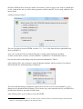
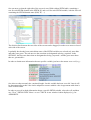
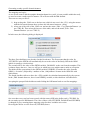
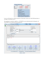
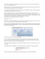
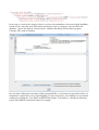
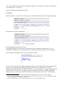
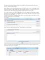
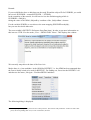
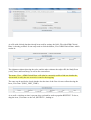
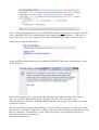
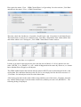
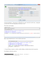
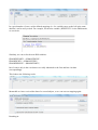
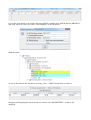
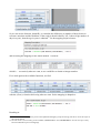
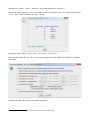
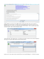
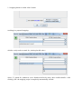
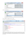
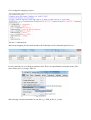
SDTM-ETL 3.0 User Manual and Tutorial
Author: Jozef Aerts, XML4Pharma
Last update: 2014-02-15
Loading an SDTM template – mappings for DM
After having loaded and inspected a CDISC ODM file with the study design, we can start working
on the mapping with SDTM or SEND.
At the left side of the screen, the tree view of the clinical study design is already shown, in this case
of the CES study1:
the right side of the screen being still empty.
In order to start mapping to SDTM (or SEND) a template which is implementing the SDTM-IG or
SEND-IG needs to be loaded. In order to do so, use the menu „File – Create define.xml“:
The reason it speaks about a define.xml is that all our mappings, and any other metadata about our
1 This is a study design originally developed by Dave Iberson-Hurst for demo purposes, and later extended by others.
SDTM or SEND will be stored in a define.xml structure, which is kept in sync with everything that
we do, so that at the end, we will be able to generate a define.xml file2 for our study with just a few
mouse clicks.
A dialog is then presented:
The user can choose between SDTM versions 1.2, 1.3 or 1.4 (the latter has been published early
2014) or SEND 3.0.
Also, one can choose between using define.xml 1.0 and 2.0 for keeping the metadata.
As these are the latest versions, we select SDTM 1.4 (SDTM-IG 3.2) and define.xml 2.0.
One can also come to this dialog using the keyboard combination CTRL-N.
After clicking „OK“, the system now starts loading the template, which can take a few minutes.
When finished, the following dialog is displayed:
The reason that this dialog is displayed is that some users like to work on the templates, e.g. for
adding newly published (draft) domains. This is pretty easy, as the template files are just XML files
which can be edited by any kind of XML editor.
After clicking „OK“ we are ready to work with SDTM...
2 For any SDTM or SEND submission, the FDA requires a define.xml file to be submitted together with the actual
data sets, containing the metadata for the submission files.
One can now see that the right side of the screen is now filled with an SDTM table, containing a
row for each SDTM domain in the SDTM-IG, and a cell for each SDTM variable, with the first cell
containing the SDTM domain name (DM, TE, ...):
The division line between the two sides of the screen can be dragged, in order to see more or less of
each side of the screen.
It probably has already been noticed that some of the SDTM variables are colored red, some blue
and other ones green. The red ones are the ones that are designated as being „required“ in the
SDTM-IG, the blue ones those that are designated as being „expected“, and the green ones those
that are „permissible“.
In order to obtain more information about a specific variable, just hover the mouse over a cell, e.g.:
One also sees that currently the „maximal length“ for this variable has been set to 80. Later it will
be demonstrated how this value can be adapted to a more suitable value in agreement with what is
in the collected data.
In order to get real in-depth information about a specific SDTM variable, select the cell, and then
use „View – SDTM CDISC Notes“ or use CTRL-H. A new window is then displayed, e.g. for
AEMODIFY:
One can then open the corresponding section of either the standard specification or implementation
guide (SDTM-IG by either clicking the button „SDTM Spec. v.1.4“ or „SDTM-IG v.3.2“,
as the latter documents come with the distribution3.
Later we will also learn how to add additional standard variables, and how to add „non-standard“
variables that later typically go into „SUPPQUAL“.
Now have a look at the first cell in a row. Also here, hovering the mouse displays some more
information, e.g.:
The label for this domain is „Morphology“, and it belongs to the „Findings“ class. The other
information will be explained later when it is explained how the domain properties can be edited.
Viewing and hiding domains
SDTM 1.4 has a lot of new domains, and it is easy to loose overview. Therefore individual domains
in the table on the right can be hidden or be displayed, so that one can concentrate on the ones that
currently are of importance. To do so, use the menu „View – View/Hide domains“:
3 One only need to set the path to the favorite PDF viewer in the „properties.dat“ file, as explained in the SDTM-ETL
installation guide.
A list of domains then is displayed, and we can check the ones that we want to keep displayed in the
table (all others are hidden). For the moment, we just keep DM (Demography) and „SV“ (Subject
visits) as these can usually best be mapped first:
After clicking „OK“, the table on the right reduces to:
Generating a study-specific domain instance
The mapping can begin...
As we do not want to edit the template domains themselves (well, it is not possible within the tool),
we need to create a study-specific instance. We will start with the DM domain.
There are two ways to do so:
1) drag-an-drop the „DM“ row to the last row (which in our case is the „SV“) using the mouse
with the left mouse button down (release the left mouse button to „drop“)
2) select one of the cells of the „DM“ row and use the menu „Edit – Copy Domain/Dataset“ (or
use CTRL-B). Then select the last row of the table, and use the menu „Edit – Past
Domain/Dataset“ (or use CTRL-U)
In both cases, the following dialog is displayed:
The three first checkboxes are already checked in advance. The first means that the value for
„STUDYID“ in the SDTM will automatically be set to the value of the Study OID in the ODM
(which is usually a wise decision).
The second will fix the value of the SDTM variable „DOMAIN“ to the one from the template. This
is almost always the case – later we will see in which cases one might want to make an exception.
The third tells the system that for the SDTM variable USUBJID, it can take the value from the
ODM, i.e. from the „SubjectKey“ attribute of the „SubjectData“ element in the ODM file with
clinical data.
The fourth checkbox allows to have the --SEQ variable be calculated automatically by the system.
In the „DM“ domain however, there is not DMSEQ variable, so this checkbox is disabled here.
Accepting the prespecified checkboxes and clicking the OK button leads to our first mappings:
One sees that a new row has been created, with the name (OID in the define-xml) „CES:DM“ for
the our study-specific DM domain. The color of three cells (STUDYID, DOMAIN and USUBJID)
is changed to grey, meaning that a mapping script for these variables now exists.
Hovering the mouse over the first cell (CES:DM) shows:
Later we will learn how to edit the properties of the domain. In the case of the DM domain there is
currently no necessity to do so.
The mapping for a specific variable (e.g. „STUDYID“) can be edited by double-clicking the cell.
This leads to a new window that opens and shows:
This window is named the „mapping editor“, which we will use a lot. Let us first look at the basic
features of this mapping editor.
The upper panel is for advanced usage when complicated selections for items must be made. It can
be hidden by using the button „Hide Upper Panel“.
The smaller panel „Mapping Description“ has already been prefilled. It contains a short description
of the mapping. Please feel free to edit its text.
The most important panel is the panel „The Transformation Script“. This is where the script is
generated and/or edited. The scripting is in a special, easy-to-learn language. Although most of the
scripts are generated automatically, it will be necessary to learn about this scripting language, which
is described in a special document „SDTM-ETL Scripting Language“.
In the current case the mapping script is very simply:
$STUDYID = “CES“;
stating the the variable STUDYID is a string (remark the quotes) with a fixed value of „CES“. Also
notice the semicolon at the end marking the end of the statement.
The lower panel „Scripting Language Functions“ contain a series of buttons for generating snippets
of coding involving build-in functions. To get more explanation about a specific function, just hover
the mouse over a button, e.g.:
We will later treat the use of functions in detail.
For very complicated mappings (which I hope is the minority – but that depends on your study
design), one can „blow up“ the central panel using the button „Full Screen Transformation Script
Panel“ which generates a full screen script editor panel.
When done editing the mapping script, click the „OK“ button, or use the „Cancel“ button to cancel
all editing.
For the DM variables „DOMAIN“ a similar mapping has already been generated automatically:
Double-clicking the cell „USUBJID“ provides the mapping for the variable „USUBJID“:
The field „Mapping Description“ has been prefilled (but you can edit that) stating that the value will
be taken from the ODM ClinicalData.
The transformation script itself uses a function usubjid(), which simply takes the value of the
„SubjectKey“ attribute of the SubjectData element in the ODM file with clinical data.
Let us now test this mapping on a real set of clinical data. For this, click the button „Test –
Transform to XSLT“. This will generate a mapping script in XSLT language4 (which you do not
need to learn) to transform XML files or to extract information from XML files such as CDISC
ODM files with clinical data.
The result of clicking the button „Test – Transform to XSLT“ is a new window:
It asks you whether your ODM clinical data is „non-typed“ or „typed“. If you don't know, ask your
EDC vendor or the source of your clinicalm data, or just try one of both possibilities (you will
immediately find out which one applies). You can also have a quick look at a file with clinical data.
In case you find a lot of „ItemData“ elements with a „Value“ attribute, this means that your data is
„untyped“. For example:
If your data however contain elements like „ItemDataString“ or „ItemDataDate“ and there is no
„Value“ attribute, this means that your data is „typed“. For example:
4 XSLT is an international standard from the W3C for transforming XML documents
In our case, we work with „untyped“ data, so we leave the radiobutton „it uses non-typed ItemData“
selected. If it is sure that your clinical data will always come as „untyped“, one can check the
checkbox „Never ask again in current session“, and then this dialog will not show up again.
Clicking „OK“ leads to a dialog:
One can then validate the correctness of the generated XSLT, or just inspect it (specialists with very
complicated scripts like to do so for debugging). In 99% of the cases, you will however just want to
continue by clicking the „Test XSLT in ODM Clinical Data“. This leads to a filechooser allowing
to pick the ODM file with clinical data. For example:
Clicking „Open“ then immediately executes the script. As our file only contains the data for a single
subject, the output is:
Notice that this testing mechanism only works for a single variable in a single domain. Later we
will learn how to do more sophisticated testing.
Let us now generate an alternative mapping for USUBJID. For example, we would like to have the
value of USUBJID to be a concatenation of the STUDYID and of the subject ID from the
„Common“ section of each form. For doing so, first select the cell „USUBJID“ and then expand the
tree with the study design so that you see an item „Subject ID“ in a group of items „Common“. One
can of course also do a search in the study design tree (see the document „Loading ODM“). For
example:
If one looks carefully, two important observations can be made:
a) the items that are visible have a green „traffic light“ in fron of them
b) the item „Subject ID“ has a traffic light that has a square around it
The green „traffic light“ means that the item is of a suitable data type for mapping to the SDTM
variable. For example, if one expects a datetime for an SDTM variable, the traffic light on the item
„Subject ID“ in the study design tree will be read5. The square around the green „traffic light“
means that the item is a „hot candidate“, i.e. has been annotated in the ODM as being ideally suited
for mapping with the given SDTM variable.
This can also be seen by hovering the mouse over the item „Subject ID“ in the study design tree:
Technically, this was done by adding the attribute SDSVarName=“USUBJID“ in the ODM.
To use the item „Subject ID“ in the mapping for the SDTM variable „USUBJID“, select the item
„Subject ID“ in the tree with the mouse, then drag it (keep the left mouse button down) to the cell
„USUBJID“ in the table on the right, then drop it by releasing the left mouse button. During the
dragging, you will see a yellow „copy“ symbol replacing your mouse cursor, meaning that you are
in the „copy“ mode.
After having dropped in the „USUBJID“ cell, the following dialog is displayed:
5 Which does not mean that it cannot be used in that mapping – people drive through red traffic lights, but that is
taking a big risk ...
as a mapping already exists for USUBJID. Select „Overwrite existing mapping“ and click „OK“.
This displays a new dialog:
The most important radiobutton is the button „Import Xpath expression for ItemData Value attribute
(from Clinical Data) meaning that we want to import a collected value (this will be >90% of the
cases). We will come to the function of the other radiobuttons later.
The lower part of the dialog states that we currently have set the maximal length for USUBJID to
60 (being the default) from the template, but that the maximal length in the study was defined to be
11. Checking the box „Set SDTM Variable Length to ODM ItemDef Length“ allows to reduce the
SDTM variable length to the one given in the study design, wich is 11.
Don't check the checkbox for now, as we still want to concatenate with the Study ID.
After clicking the OK button, the mapping scripting shows up:
Essentially what is does, is to define a path to the item in the clinical data, and store the result in the
variable $USUBJID. As it is a path in XML, this is called an „XPath“ expression.
One can now test this script again on clincal data (as before), giving the same result as before.
Now we want to concatenate the value of STUDYID with the above result. In order to do so, we
need to adapt the script slightly. First, the variable $USUBJID is renamed into $TEMP. We then
have:
Do not change anything in the „XPath“ expression6.
Now, we do already have a mapping for the SDTM variable $STUDYID. We can just copy-paste
from the previous mapping which results in:
Now have a look at the functions in the lower panel, the „Scripting Language Functions“ panel. You
will find a „concat“ function with the following explanation:
6 It will be very seldom that one needs to change something in the XPath expression. We will give some examples
later though
The „concat“ function has at least two arguments, but there can be more. It is used to concatenate a
set of strings into a new string.
Now in the mapping script editor, just type:
$USUBJID =
and then click the „concat“ button. The string is extended with the function with empty parameters:
which can now easily be extended as:
Do not forget the semicolon at the end7.
You might already have noticed the coloring in the script: comments (starting with a „#“) are
colored blue8. Functions are colored green, and strings (that are between quotes) are colored red.
Reexecuting the mapping script on real clinical data results in:
One can also execute all the available mappings together. After clicking OK for the mapping script
editor, we come into the main window again. Now, use the menu „Transform – Generate
Transformation (XSLT) Code for CDISC-SDS XML“ or use „Transform - Generate Transformation
(XSLT) Code for SAS-XPT“. The former will generate data files in the new CDISC SDS-XML
format, the latter in the classic SAS-XPT format. Let us first try the classic way9. The following
7 If the semicolon is forgotten, a warning message will be displayed when trying to execute the mapping.
8 As in every programming effort, it is advised to add as many comments as possible, for a later good understanding
what the intention of the statement or snippet was.
9 Later, it will explain how to do the same generating results in the new SDS-XML format.
dialog is presented:
One can now save the transformation XSLT code to file10, but we will execute the code within the
software itself, so click „Execute Transformation (XSLT) Code“. This results in a new dialog:
10 This can be useful to execute the transformations off-line.
The upper field allows to add the location of the ODM file with clinical data. One can use the
„Browse“ button to locate this file.
At the moment, we do not need to generate any SAS-XPT files, so we leave the checkbox „Save
Result SDTM tables as SAS XPORT files“ unchecked. The checkbox „View Result SDTM files“
remains checked – this will open an own viewer for the results that we have sofar.
One of the advantages of the SDTM-ETL software is that one can start developing the mappings
even before the first subject has enrolled. But in order to test the mappings, we need some clinical
data, even if it are mock data.
Consider the case that we already have some (but not all) collected data of a first subject. We can
already use these data to test our mapping.
For example:
and we can now click the button „Execute Transformation on Clinical Data“
After a few seconds, the transformation has been executed, and a new window with the results
(those that we have sofar) is displayed:
Remark:
If you would liked to have a dash between the study ID and the subject ID for USUBJID, you could
have used: $USUBJID = concat($STUDYID, '-', $TEMP);
In the remaining of the tutorial, we will however use the default mapping which is:
$USUBJID = usubjid();
taking the value of the ODM „SubjectKey“ attribute of the „SubjectData“ element.
For the variable SUBJID, we can also use the same mapping $USUBJID=usubjid();
but you can also decide otherwise.
The next variable is RFSTDTC (Reference Start Date/time). In order to get more information on
this item use CTRL-H or the menu „View – SDTM CDISC Notes“. This displays the window:
We can easily map this to the date of the first visit11.
Maybe there is a „hot candidate“ in the ODM for RFSTDTC, i.e. the ODM has been annotated that
the item is ideally suited to be used for RFSTDTC. For finding out, first select the RFSTDTC cell
and then use the menu „Navigate – Find hot SDTM Candidate“:
The following dialog is displayed:
11 Our very simple sample study does not have a data point for „date of first study treatment“. If there is such a data
point, the corresponding date can (or even is advised to) be used.
One can select to search using the „SDSVarName“ in the ODM, the CDASH name and/or the
„SDTM Alias“.
After clicking „Find“, and if there is a „hot candidate“ in the ODM, the tree will automatically
expand, and the „hot candidate“ item is displayed and selected:
But, are there already any clinical data for this data point? One can test using the menu „View –
ODM Clinical Data“. This shows the window:
As a file with clinical data has already been used for testing, the field „File with ODM Clinical
Data“ is already prefilled. So one only need to click the button „View ODM Clinical Data“ which
results in:
The rightmost column showing the value, and the other columns the subject ID, the StudyEvent
(visit), Form, and ItemGroup, as well as the current Item.
The menu „View – ODM Clinical Data“ will often be extremely useful to find out whether the
current item is really the one we need or want for the mapping.
The same can be applied to check whether also the time of the first visit was collected using the
Item „Visit Time“ (OID I_VISIT_TIME):
As as well a visit date as time is present, they can both be used to populate RFSTDTC. To do so,
drag the item „Visit Date“ to the cell „RFSTDTC“, leading to:
and rename $DM.RFSTDTC into „$VISITDATE“.
Then drag-and-drop the item „Visit Time“ to the same cell RFSTDTC. The following wizard is
displayed:
We want to append to the existing mapping, but as we still need to combine both items, we choose
to rename the current one, e.g. to $VISITTIME:
You do not need to add a „$“ in front of the new variable name, the system will take care of it.
This results in a mapping:
Remark that the two comment lines have been generated automatically.
The SDTM Implementation Guide explains the usage of ISO-8601 dates, times and datetimes. In
case of a complete datetime, the format is: YYYY-MM-DDThh:mm:ss. The central „T“ separating
the date part from the time part. So for our mapping, we can use:
$DM.RFSTDTC = concat($VISITDATE, 'T', $VISITTIME);
Hey, wait a minute! What in the case that the visit time was not collected? Then the central „T“
should not be present! So … time for our first if-else statement!
Like for the „concat“ function, one can use the „if“, „elsif“ and „else“ buttons from the „Scripting
Language Functions“ panel to insert snippets:
e.g. leading to:
One can then fill in the individual parts:
The „if“ statement saying that in case the VISITTIME variable is not empty („!=“ symbol), then the
value of DM.RFSTDTC is the concatenation of the visitdate with the characted „T“ and the visit
time. In any other case („else“ statement), the value of DM.RFSTDTC only consist of the date.
Testing on our single subject leads to:
The next SDTM variable that needs to be mapped is RFENDTC (Reference end date/time). Using
CTRL-H tells us:
But now the question arises: what was the date the subject ended the trial? Was it the „Week 2
Visit“, or was it the „Patient Diary Event“, or maybe even the „Adverse Event“ visit?
This time the menu „Navigate – Find hot SDTM Candidate“ does not give any results, so we need
to find out ourselves...
We can easily find out what the last visit date is, as it was always collected (i.e. in each visit) using
the same item („Visit date“, with OID „I_VISIT“). One can easily see this by selecting the item, and
then use „Navigate – Next Instance“ (or use CTRL-Page-down). One will then see that it was
collected for each form for each visit.
But what was the last one?
Here again, the menu „View – ODM Clinical Data“ is of great help. So select an item „Visit Date“
and then use the menu „View – ODM Clinical Data“:
This time, check the checkboxes „Generalize for all Forms“ and „Generalize for all StudyEvents“.
This means that we want to see each data point „Visit Date“ independent from within which form
and within which visit. Clicking the „View ODM Clinical Data“ button leads to:
showing all the visit dates ever registered.
It looks as (at least for this subject) the last visit date was on March 13th 2010, and the visit was
either „WEEK_2“ or „DIARY“ or „AE“, which all happened on the same day. However, we cannot
know whether this will apply to all subjects.
The ODM standard states that clinical data for subjects MUST come in chronological order, with
earliest data first, and latest data last in the file. So we can simply look for the last occurrence of
„Visit Date“ for each subject in the file with clinical data.
After having gone back to the main window, drag-and-drop one of the items „Visit date“ from the
tree with the study design (it doesn't matter which one), and drop it in the cell „RFENDTC“. The
following dialog is displayed:
Check the checkboxes „Generalize for all StudyEvents“ and „Generalize for all Forms“, stating that
we want to have the item independent of the form or visit12.
This leads to the mapping:
But we only want the last one, so we do a little rewrite into:
i.e. By generating a temporary variable, and then adding a condition [last()] to the expression13.
Executing the script then results in:
12 Later we will see how to work with the buttons „Except for ...“ and „Only for ...“
13 „take the first one available“ is written as „[1]“
In a good number of cases, earlier defined mappings (i.e. for variables more to the left in the same
domain) can be easily reused. For example, for the next variable „RFXSTDTC“ in the DM domain,
we can write:
Similarly, we can set for the next DM variables:
$DM.RFXENDTC = $DM.RFENDTC;
$DM.RFICDTC = $DM.RFSTDTC;
$DM.RFPENDTC = $DM.RFENDTC;
but of course only in the case dates were really indentical to the first and last visit date
correspondingly.
This leads to the following result:
Meanwhile we have received the data of a second subject, so we can test our mapping again:
Resulting in:
Let us now concentrate on two other important SDTM variables in the SDTM domain: BRTHDTC
and AGE. Again we first try to find a „hot candidate“ in our ODM tree.
With the result:
A view in the clinical data for this item (using „View – ODM Clinical Data“) results in:
Dragging and dropping the item from the tree into the cell „DM.BRTHDTC“ results in the
mapping:
and doing a „local“ quick test of this mapping results in:
Or executing the mapping for all SDTM variables in the DM that we mapped sofar in:
The next variable that needs to be mapped is „AGE“. However, it looks as the age of the subject
was not collected directly, so we need to calculate it from the birth date and the reference start date.
Just double-click the cell „AGE“ to start the mapping process:
As the birth date ($DM.BRTHDTC) and the reference start date ($DM.RFSTDTC) were already
mapped before, we can reuse them, but in only in „read mode“.
Now look into the lower part of the mapping screen, where the „Scripting Language Functions“ are
displayed. If we scroll down, we find:
So we can use the function „datediff()“ to calculate the difference (in number of days) between
reference start date and the birth date. If the result is then divided by 365.2 (the average number of
days in a year), then the age in years is obtained14. So the mapping script becomes:
and executing the mapping for the whole domain15 results in:
which is … not entirely what we want, as we would like to obtain an integer number.
If we look again to the available functions, we find:
with the „floor()“ function delivering what we want. So the mapping is adapted to:
Resulting in:
14 Of course one can develop more precise and sophisticated mapping scripts for the age, but this is out of the scope of
the current tutorial.
15 We can not do a „local“ testing, as the variables „DM.RFSTDTC“ and „DM.BRTHDTC“ are out of scope, as they
have been defined in previous mappings.
which is exactly what we want.
This kind of calculations should be the exception in SDTM, as SDTM is about collected data and
not about derived data. Unfortunately, derivations have sneaked in in SDTM in the last years, as the
tools of the regulatory authorities are not able to calculate them „on the fly“ from the already
available data. A typical example are all the --DY variables.
The next SDTM variable is „AGEU“. In our case it just is the string „YEARS“. So the mapping is:
For „SEX“, we once again first look for a „hot candidate“ and find:
It is seen that the „traffic light“ is blue, meaning that the variable is under controlled terminology.
The information about the SDTM controlled terminology can be obtained using the menu „View –
SDTM associated codelist“ which delivers:
standing for „female“, „male“, „unknown“ and „undifferentiated“ (intersex)16.
Also on the ODM side, there is an associated codelist. Selecting the item „Sex“ and using the menu
„View – Item CodeList details“ provides a dialog:
stating that in the ODM, only the values „M“ and „F“ are foreseen.
Drag-and-drop from the item „Sex“ in the study design tree to the SDTM cell „DM.SEX“ displays
the wizard:
and then clicking „OK“ leads to the following dialog:
16 See the published CDISC controlled terminology lists published by NCI
asking whether we want to use the ODM codelist (coded or decoded values), the currently to
DM.SEX asscociated codelist, or another list from the SDTM define.xml list. We want to use the
SDTM codelist, so we select „Use codelist from the SDTM Variable“. We can quickly inspect that
codelist using the „Show CodeList Details“ button:
After clicking the „OK“ button in the „A CodeList is associated“ wizard, a new wizard is displayed
allowing us to map the ODM codelist with the SDTM codelist:
In this case it is easy, and even the wizard will have an easy task finding out – so click the „Attemp
1:1 mapping based on coded value“ button:
resulting in a proposal mapping:
which we only need to extend for „missing/invalid value“:
where „U“ stands for „unknown“ as we found out before by using „show codelist details“. After
clicking „OK“ the mapping script is completely automatically created:
the „if-elsif-else“ construct being generated automatically.
In many cases, wizards will create mapping scripts completely automatically, but the user can
always further enhance or change the mapping script manully.
A similar mapping needs to be done for „RACE“. Using the menu „Naviage – Find hot SDTM
Candidate“, the ODM item „Race“ is quickly found in the study design tree“, and the subsequent
drag-and-drop leads to:
and the codelist mapping wizard:
which is easily mapped to:
The two ODM entries mapped to „NULL“ (empty).
This leads to the automatically generated mapping script:
„Other“ is not part of the official CDISC codelist, but we could of course add it (later we will see
how), and add it to the mapping script. In that case, depending on whether the study design had also
a „please specify“ field, one should also add a supplemental qualifier to provide the information on
the „other race“.
If we change the mapping script to:
and test the mapping for the whole domain, the following result is obtained (partial view):
It's not a bad idea to save all the work done sofar. This is accomplished by using the menu „File –
Save define.xml“ (or using CTRL-S):
and selecting a location and name for our file, e.g. „DM_define_2_0.xml“:
The „Country“ is fixed in this study. So one can just add $DM.COUNTRY = 'xxx' where 'xxx' is the
three character code in ISO-3166 notation. Examples are: USA (United States of America), CAN
(Canada), GER (Germany), AUT (Austria), AUS (Australia).
The next variable is DMTDC. When using CTRL-H, more information is displayed:
We can just take it as the „Visit Date“ for the form where also the demographics data was collected:
In this case, a simple drag-and-drop from the item „Visit date“ is all is needed.
The next one is DMDY:
There is something very special (see the SDTM-IG). In SDTM, the day the study starts for a
specific subject has xxDY = 1 (and not 0 as one might think). The day before the study starts
however is then not day 0, as one might think, but day -1. So in SDTM, there is no day „0“, and
xxDY can never have the value „0“. Logical, isn't it17?
So when calculating xxDY, we must always add logic in our script to avoid that a value „0“ is given
as the result. In this case, it is pretty simple – we can even reuse variables that were defined before.
For DMDY, we write the mapping:
DM.DMDTC and DM.RFSTDTC have been defined before (i.e. more to the left), so we can reuse
them in „read only“ mode. The „datediff()“ function delivers the difference in days. In case the first
parameter value is later than the second, a positive (or better said, non-negative) result is obtained.
One immediately sees that this can lead to a DMDY=0 result when DMDTC and RFSTDTC are
identical (as is the case)18. So we adapt the mapping to:
There is one pecularity in this script: the „datediff“ function essentially returns a string19, which
need to be transformed into a number (kind of casting) in order to do mathematical calculations
with it.
The result for our two subjects is:
17 That was meant sceptically ...
18 Essentially, DMDY should never appear in SDTM, as SDTM is about collected data, not about derived data. The
tools of the FDA should do these kind of calculations.
19 The reason for this is that in XSLT, a datediff returns a duration, e.g. „P1D“ meaning a period of 1 day.
In the next chapter, we will work on the SV (subject visits) domain, and also introduce a new output
format, and an alternative (better) viewer for inspecting the resulting records.