Download Servomotor Open-loop Frequency response and Transfer Function

LAB 5
SERVOMOTOR OPEN LOOP FREQUENCY RESPONSE
AND TRANSFER FUNCTION ESTIMATION
1. LAB OBJECTIVE
The purpose of this lab is to experimentally determine the frequency response of a DC servomotor
system. Experimental data will be obtained to create a Bode plot for the open loop frequency
response of a DC servomotor and determine the transfer function of the system. Once the transfer
function for the system is known, suitable controllers for the system can be derived.
2. BACKGROUND
2.1. Introduction to the DC Servomotor System
Figure 1. Servomotor drive system
A DC brush-type servomotor is used in the lab. The specifications of the motor and amplifier
are as follows.
2.1.1. Bi-directional servomotor
Function:
Manufacturer:
Model number:
Maximum speed:
- Continuous torque:
- Peak torque:
Weight:
- Torque constant:
Recommended supply voltage:
- Armature resistance:
To supply rotational energy to the system
Galil
N23-54-1000
5900 rpm
0.38 Nm
2.95 Nm
1.7 Kg
0.096 Nm/A
60 V
1.8 Ω
1
- Armature inductance:
- Electrical time constant:
- Electro mechanical time constant:
4.1 mH
2.27 ms
8.8 ms
2.1.2. Encoder (comes attached with the motor)
Function:
Manufacturer:
Cycles per revolution:
Inertia:
To detect shaft position
Galil
1000 ppr (pulses per revolution)
2.6x10-5 oz-in-sec2
2.1.3. Servo Amplifier
Function:
Manufacturer:
Model number:
To supply power to drive the motor
Galil
MSA-12-80
Has protection against over-voltage, over-current, over-heating, and short circuits across motor,
ground and power leads. Has adjustable gain.
2.1.4. Power supply
Function:
Manufacturer:
Model number:
Power rating:
To provide DC supply voltage to the amplifier
Galil
CPS-12-24
24 VDC @ 12 A
2.1.5. System model
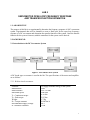
A block diagram of the DC servomotor system, which is typical, is shown in Figure 2. The
power amplifier shown is a voltage amplifier in which the input and output is a voltage. Servo
systems could use current amplifiers instead. The voltage amplifier is modeled as a gain
and
), a low pass filter of sorts. The variable represents the Laplace operator.
a lag (
2
Figure 2. Block diagram of the DC servomotor system
The servomotor can be modeled as a second order system. As shown in the Figure 2, the
motor gain is the reciprocal of the voltage constant
. The electrical time constant
is 2.27
ms, according to manufacturer specifications.
represents the mechanical time constant of
the unloaded motor and is specified to be 8.8 ms. Since the servomotor is connected to an
encoder and a coupling, the actual mechanical time constant
is larger than the specified
value of 8.8 ms.
A counter is required to monitor the output of the encoder. In our case, the Sensoray I/O card
has counters that keep track of encoder pulses. The encoder-counter is modeled as an
integrator
, where
is the resolution of the encoder and
is an integrator
represented in the Laplacian domain.
Figure 2 shows an open loop diagram of a servomotor system. The shaft encoder signal can be
used as feedback to create a closed loop position control system. For closed loop velocity control,
the derivative of the encoder signal would be used as feedback. We will implement closed loop
position and velocity control systems in the next lab.
It turns out that the amplifier dynamics (
) can usually be neglected, and the motor
and load can be lumped together as a second order system. The open loop diagram of the servomotor
system can be simplified as shown in Figure 3. (Refer to Ogata’s “Modern Control Engineering”,
Section 4-3, pg. 141 for further details on modeling second order systems.)
Figure 3. Lumped open loop diagram of a DC servomotor system.
2.2. Second Order Servo System Model:
It turns out that the DC servomotor system used in the lab can be simplified even further. An
acceptable second order model for this system is shown in Figure 4.
3
Figure 4. Simplified open loop diagram of the DC servomotor system.
Here,
is the net gain of the system and
is the electro-mechanical time constant of the
system. ( ) is the Laplace variable of the angular position and ( ) is the Laplace variable of
the input voltage to the system. The Bode plot for this transfer function is shown below.
Figure 5. Bode plot for the transfer function
( )
( )
(
)
2.3. Experimental determination of the servomotor transfer function
2.4. Position sensing
The lab experiments require accurate servomotor shaft position sensing. The position sensor
that is available in the lab is an incremental encoder-counter arrangement. The incremental
encoder resolution is 1000 counts per revolution. Since the encoder shaft is connected directly to
the servomotor shaft, the encoder can detect 360/1000 = 0.36 degree change in motor shaft
rotation.
The encoder is connected to the counter in the Sensoray I/O card. The card has six counters
arranged in three pairs: 1A, 1B, 1G, 2A, 2B and 2G. The features include:
 24-bit up/down counters.
4
 Counters can be completely software driven.
 Counters can be driven from digital inputs 1-16.
 Counters can be driven from the internal clock creating timers.
 Counters can be driven from encoder inputs (our mode of operation).
 Encoder quadrature multiplier (x1, x2, x4).
 Selectable counter direction for timer and event counting modes.
 5 Volt encoder power is available at the encoder connector.
There are several modes in which the counters could be used. Typical choices are:
 The counter is driven by an encoder pulse or internal clock or by digital input.
 Up counting or down counting using the system clock
 Encoder quadrature multiplier (x1, x2, x4) etc.
The required mode of operation is chosen by setting registers GR1A and GR1B to the appropriate
value. For example to drive the counter with an “encoder signal” in “unit multiplier” mode, we set
GRA1 = 0x0360 and GRB1 = 0x0C50. The register values for other modes of operation can be
identified from the user manual of the I/O card.
The following lines of code can be used for reading in the encoder signal:
#include <stdio.h>
#include <conio.h>
#include <wtypes.h>
#include <winbase.h>
#include <mmsystem.h>
#include "Win626.h"
#include "App626.h"
#define CRA1
0x00
#define CRB1
0x02
#define PRE1ALSW
0x0C /* register offset values */
#define PRE1AMSW
0x0E
#define LATCH1ALSW 0x0C
#define LATCH1AMSW 0x0E
typedef DWORD HBD;
void main(void)
{
HBD hbd = 0;
WORD ldata, hdata; /* unsigned short (16bits) */
int enc_count; /* where encoder data is stored */
int start_count; /* remember beginning count */
printf("\nEncoder test\n\nManually turn the motor shaft\n\nhit any key to
quit\n\n");
/* initialize the Sensoray 626 board */
S626_DLLOpen();
S626_OpenBoard( hbd, 0, 0, 3);
/* counter initialization */
S626_RegWrite(hbd,PRE1ALSW,0x0000);
S626_RegWrite(hbd,PRE1AMSW,0x0080);
5
S626_RegWrite(hbd,CRA1,0x016f);
S626_RegWrite(hbd,CRA1,0x0360);
S626_RegWrite(hbd,CRB1,0x0C50);
/* read in low 16 bits into variable ldata */
ldata = S626_RegRead(hbd, LATCH1ALSW);
/* read in bits 23 to 16 into variable hdata */
hdata = S626_RegRead(hbd, LATCH1AMSW);
/*left shift hdata by 16 bits */
enc_count = ((int) hdata) << 16;
start_count = enc_count | ((int) ldata);
while(!kbhit())
{
ldata = S626_RegRead(hbd, LATCH1ALSW);
hdata = S626_RegRead(hbd, LATCH1AMSW);
enc_count = ((int) hdata) << 16;
enc_count = enc_count | ((int) ldata);
enc_count -= start_count; /* so we begin from 0 */
putchar('\r');
printf("%10d", enc_count);
}
S626_CloseBoard( hbd );
S626_DLLClose();
} /* end of main */
Program details:
The “#define” statements assign the appropriate memory addresses to the register. Each register
has a hexadecimal address value specified as an offset value from the base address of the I/O
board. The offset values for various registers are given in the Sensoray user manual. For example,
register CRB1 has an offset of 0x02. If the base address of the card is 0x5000, then the actual
address of the register variable is 0x5002.
S626_RegRead:
S626_RegWrite:
Reads values from registers and stores the values in a variable.
Writes a specified value to a register.
A pulse from the encoder causes a 24-bit register to be incremented by one. However, only 16
bits can be read from the counter registers at a time, so we first read the low 16 bits into a
variable ldata and then read the remaining 8 bits into the variable hdata. For example, if the
encoder reading is 0x32A3B1, ldata contains “0xA3B1” and hdata contains “0x0032”. The
two values are then merged to form a 24-bit word. (The operation is similar to the bit-merge
program you wrote in Lab 3).
2.5 Drift Removal
After an entire motor encoder reading sequence is generated and recorded into an array, you
need to call the function high_pass_filter in your program to filter out the low-frequency drift
component from the measurement data. The source code for this function is included in lab6.c.
Both lab6.c and its corresponding header file lab6.h will need to be included in your Visual Studio
project to use this function. They can be downloaded from the course website.
6
The description of the function high_pass_filter is given below:
int high_pass_filter(int *original_data,double *filtered_data,
int element_number, double f);
*original_data:
*filtered_data:
element_number:
f:
pointer to the array that saves the original measurement data.
pointer to the array that the filtered measurement data is saved to. It has
the same number of elements as the original_data array. It is assumed that
this array is created in the main program.
number of elements in original_data array.
frequency of signal output from ADC in Hz.
For a detailed explanation of this preprocessing and why it is necessary, please refer to the
appendix at the end of this handout.
2.6 Save Encoder Data
After filtering the encoder readings, they can be saved to a text file by calling the function
save_enc_data shown below:
int save_enc_data(double *filtered_data,int element_num)
The input arguments *filtered_data and element_num should be the same variables that were used
during data filtering. This function will create a text file titled “enc_data.txt” that contains the
filtered data. The source code for this function is also included in lab6.c.
3. PRELAB ASSIGNMENT
1. Study this handout and related lecture material. In Bolton, read the following:



Section 7.5 DC Motors, pp. 168-176.
Section 9.3.2 System Models: D.C. Motor (pp. 214-217).
Chapter 12 Frequency Response (pp. 262-277).
2. Write a program that produces a sinusoidal voltage output at DAC0 at a user specified
frequency and amplitude. You will use the output of this program as an input to the
servomotor. This way we can observe the response of the servomotor system to different
input (drive) frequencies and amplitudes. The program should also read in the encoder
signal from the servomotor (see section 6.2.4). Use a sampling frequency of 1000 Hz and
test duration of 10s when collecting data from the encoder. At the end of the program, the
encoder signal should be filtered (see section 6.2.5) and stored to a text file (see section
6.2.6).
3. Write a Matlab program that calculates the peak-to-peak value of the servomotor shaft
7
oscillation. The program must be fully documented with meaningful comments. Your
program should load an array of 10000 elements (i.e. the filtered encoder readings) from
the file “enc_data.txt” and calculate the peak to peak value. (Hint: One way is to identify
the maximum and minimum value of the encoder signal over a number of cycles, for
example 20. Then take the average to identify the average peak-to-peak displacement value.
Another method is to use RMS detection. Take the RMS value of a portion of the encoder
signal and then multiply by √ to calculate the average peak-to-peak displacement value)
NOTE: In the lab you will use the above two programs such that the program oscillates the
shaft while simultaneously collecting the encoder data. The program will send the encoder
data to a high pass filter and then store the filtered data in a text file. The Matlab program you
wrote for Exercise 3 is to get the encoder oscillation amplitude necessary to create the
experimental bode plot of the system.
4. LAB PROCEDURE
In this lab we will determine the frequency response of the plant by applying a sinusoidal input
voltage and recording the amplitude of the motor shaft position as a function of frequency.
First, connect the DACO channel to the input of the servomotor. In your program (tested with
the oscilloscope first) set the drive frequency to be equal to 5Hz and set the amplitude of the
driving signal to be 0.5V amplitude. Execute your program. Using your Matlab code from
prelab exercise 3, calculate the peak-to-peak value of shaft oscillations. Write clown this
value. Repeat the above procedure for the different drive frequencies listed in the table at the
end of the lab handout.
Repeat the experiments for 1V amplitude sine wave input.
5. POSTLAB ASSIGNMENT AND LAB REPORT
1. Create bode plots (magnitude only, log-log plots) of the open loop frequency response of
the plant. Use the data obtained from the experiments with 0.5V and IV sine waves. Plot
both plots on one graph for comparison. Discuss the differences and similarities. What do
you expect in terms of the similarity of these plots and what did you get? What do you think
might be the reason if there is an inconsistency?
2. Based on the frequency response shown by the bode plots, estimate the open loop transfer
function of the plant. Assume the transfer function has the form illustrated in Figure 5.
Your plots should be similar to this figure. The gain
is the value of the y-ordinate where
the experimental curve crosses the
rad/s line. The frequency
is the point where
the plot transitions from a –20 dB/dec line to a –40 dB/dec line. Then
. Obtain
transfer functions for both 0.5 V inputs and 1.0 V input. Compare the two transfer
functions.
8
Lab report requirements
1. Answers to the two above questions and the plots of Postlab question 1. Show your work for
question 2 on these plots.
2. Hardcopy of your commented C Program and Matlab program.
3. Complete record of measurement data.
9
Experimental results of the open loop plant frequency response for 0.5 V sinusoidal input.
FREQUENCY
(Hz)
MOTOR SHAFT
DISPLACEMENT
(peak to peak counts)
MAGNITUDE
20 log (output/input)*
2.5
5
10
15
20
25
30
35
40
45
50
55
60
65
70
75
*output = peak-to-peak shaft oscillation in encoder counts, input = peak-to-peak voltage.
10
Experimental results of the open loop plant frequency response for 1.0 V sinusoidal input.
FREQUENCY
(Hz)
MOTOR SHAFT
DISPLACEMENT
(peak to peak counts)
MAGNITUDE
20 log (output/input)*
2.5
5
10
15
20
25
30
35
40
45
50
55
60
65
70
75
*output = peak-to-peak shaft oscillation in encoder counts, input = peak-to-peak voltage.
11
Appendix A: Removing Drift Component from Encoder Reading
by High-Pass Filtering
A.1. Introduction
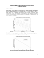
In this lab the motor is running in an open-loop mode. Under a sinusoidal signal input, a
perfectly linear system will give a sinusoidal output if it is stable. However, the DC
motor system used is marginally stable (refer to Figure 4). Since the actuation signal
typically has a small DC component, a low-frequency drift component is usually
observed in the experiments, as shown in Figure A.1. (Depending on the input signal, the
curve can also be ascending.)
Figure A.1. Low-frequency drift component under a large sinusoidal actuation
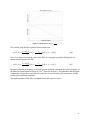
Such drifts can make accurate detections of peaks difficult when the sinusoidal signal is
small compared with the drift component, as shown in Figure A.2.
Figure A.2. Low-frequency drift component under a small sinusoidal actuation
12
In the function high_pass_filter, a high-pass filtering technique is used to remove the
low-frequency drift component so that the processed data will be in a form similar to the one
shown in Figure A.3.
Figure A.3. Encoder reading signal after high-pass filtering
A.2. High-Pass filter design and implementation
There are many different ways to design a high-pass filter. Here a simple design method is
used. First, an analog high-pass filter is designed based on the input signal. Then it is
discretized using a bilinear transformation. Here the following first order high-pass filter is
chosen.
( )
Its Bode plot when
(A1)
is shown in Figure A.4.
By using the bilinear transformation,
(A2)
we get the following discrete transfer function for the filter.
( )
(
(
) (
)
) (
)
(A3)
13
( )
Figure A.4. Bode plot for
We can then write the filter equation in an iteration form:
(
)
( )
[ (
)
( )]
(A4)
Now, if we want to increase the order of the filter, we can again use double filtering like was
demonstrated in the previous lab.
(
)
( )
[ (
)
( )]
(A5)
In order to improve the accuracy of the peak-to-peak amplitude estimation, the corner frequency of
the filter has been designed to always be 1/10th of the test frequency. This guarantees that all signal
components at frequencies more than a decade below our test frequency do not interfere with the
peak-to-peak amplitude estimation.
The implementation of this filter is straightforward and is given in lab6.c.
14