Download ABI PRISM® 3100 Genetic Analyzer User`s Manual

ABI PRISM® 3100 Genetic Analyzer
User’s Manual
© Copyright 2001, 2010 Applied Biosystems
For Research Use Only. Not for use in diagnostic procedures.
NOTICE TO PURCHASER
This instrument, Serial No. ________________, is Authorized for use in DNA sequencing and fragment analysis. This Authorization is included in the
purchase price of this instrument and corresponds to the up-front fee component of a license under process claims of U.S. patents and under all
process claims for DNA sequence and fragment analysis of U.S. patents now or hereafter owned or licensable by Applied Biosystems for which
Authorization is required, and under corresponding process claims is foreign counterparts of the foregoing for which an Authorization is
required. The running royalty component of licenses may be purchased from Applied Biosystems or obtained by using Authorized reagents purchased from Authorized supplier in accordance wit the label rights accompanying such reagents. Purchase of this instrument does not itself convey to
the purchaser a complete license or right to perform the above processes. This instrument is also licensed under U.S. patents and apparatus and system
claims in foreign counterparts thereof. No rights are granted expressly, by implication or by estoppel under composition claims or under other process
or system claims owned or licensable by Applied Biosystems. For more information regarding licenses, please contact the Director of Licensing at
Applied Biosystems, 850 Lincoln Centre Drive, Foster City, California 94404.
The ABI PRISM® 3100 Genetic Analyzer includes patented technology licensed from Hitachi, Ltd. as part of a strategic partnership between
Applied Biosystems and Hitachi, Ltd., as well as patented technology of Applied Biosystems.
ABI PRISM and its design, Applied Biosystems, BioLIMS, GeneScan, Genotyper, and MicroAmp are registered trademarks of Applied Biosystems or its
subsidiaries in the U.S. and certain other countries.
ABI, BigDye, Factura, Hi-Di, POP, POP-4, and POP-6 are trademarks of Applied Biosystems or its subsidiaries in the U.S. and certain other countries.
AmpliTaq is a registered trademark of Roche Molecular Systems, Inc.
Microsoft, Windows, and Windows NT are registered trademarks of the Microsoft Corporation in the United States and other countries.
Oracle is a registered trademark of the Oracle Corporation.
pGEM is a registered trademark of Promega Corporation.
All other trademarks are the sole property of their respective owners.
Applied Biosystems vast distribution and service network, composed of highly trained support and applications personnel, reaches into 150 countries on
six continents. For international office locations, please call our local office or refer to our web site at www.appliedbiosystems.com.
Record information about your software below.
Software CD
3100 Software
Oracle® for NT
GeneScan® Application
Sequencing Analysis Application
Serial Number
Version Number
Registration Code
Contents
1 Introduction and Safety
Overview . . . . . . . . . . . . . . . . . . . . . . . . . . . . . . . . . . . . . . . . . . . . . . . . . . . . . . . . . . . . . . . . . . 1-1
ABI PRISM 3100 Genetic Analyzer . . . . . . . . . . . . . . . . . . . . . . . . . . . . . . . . . . . . . . . . . . . . . . 1-2
To Get Started Quickly . . . . . . . . . . . . . . . . . . . . . . . . . . . . . . . . . . . . . . . . . . . . . . . . . . . . . . . . 1-3
Additional Documentation . . . . . . . . . . . . . . . . . . . . . . . . . . . . . . . . . . . . . . . . . . . . . . . . . . . . . 1-4
Safety . . . . . . . . . . . . . . . . . . . . . . . . . . . . . . . . . . . . . . . . . . . . . . . . . . . . . . . . . . . . . . . . . . . . . 1-5
2 System Overview
Overview . . . . . . . . . . . . . . . . . . . . . . . . . . . . . . . . . . . . . . . . . . . . . . . . . . . . . . . . . . . . . . . . . . 2-1
Section: 3100 Instrument Overview . . . . . . . . . . . . . . . . . . . . . . . . . . . . . . . . . . . . . . 2-3
ABI PRISM 3100 System Components . . . . . . . . . . . . . . . . . . . . . . . . . . . . . . . . . . . . . . . . . . . . 2-4
What the Instrument Does . . . . . . . . . . . . . . . . . . . . . . . . . . . . . . . . . . . . . . . . . . . . . . . . . . . . . 2-5
How the Instrument Works. . . . . . . . . . . . . . . . . . . . . . . . . . . . . . . . . . . . . . . . . . . . . . . . . . . . . 2-6
Section: Instrument Hardware Overview . . . . . . . . . . . . . . . . . . . . . . . . . . . . . . . . . . 2-9
Front View . . . . . . . . . . . . . . . . . . . . . . . . . . . . . . . . . . . . . . . . . . . . . . . . . . . . . . . . . . . . . . . . 2-10
Front View with Doors Open . . . . . . . . . . . . . . . . . . . . . . . . . . . . . . . . . . . . . . . . . . . . . . . . . . 2-11
Back View. . . . . . . . . . . . . . . . . . . . . . . . . . . . . . . . . . . . . . . . . . . . . . . . . . . . . . . . . . . . . . . . . 2-12
Section: Computer and Software Overview . . . . . . . . . . . . . . . . . . . . . . . . . . . . . . . 2-13
Computer Workstation . . . . . . . . . . . . . . . . . . . . . . . . . . . . . . . . . . . . . . . . . . . . . . . . . . . . . . . 2-14
Software . . . . . . . . . . . . . . . . . . . . . . . . . . . . . . . . . . . . . . . . . . . . . . . . . . . . . . . . . . . . . . . . . . 2-15
Section: Chemistry Overview . . . . . . . . . . . . . . . . . . . . . . . . . . . . . . . . . . . . . . . . . . 2-17
Supported Dye Sets . . . . . . . . . . . . . . . . . . . . . . . . . . . . . . . . . . . . . . . . . . . . . . . . . . . . . . . . . 2-18
Labeling Chemistries . . . . . . . . . . . . . . . . . . . . . . . . . . . . . . . . . . . . . . . . . . . . . . . . . . . . . . . . 2-19
Polymers . . . . . . . . . . . . . . . . . . . . . . . . . . . . . . . . . . . . . . . . . . . . . . . . . . . . . . . . . . . . . . . . . . 2-20
Injection Solution . . . . . . . . . . . . . . . . . . . . . . . . . . . . . . . . . . . . . . . . . . . . . . . . . . . . . . . . . . . 2-21
Section: Electrophoresis Overview . . . . . . . . . . . . . . . . . . . . . . . . . . . . . . . . . . . . . . 2-23
Capillary Array. . . . . . . . . . . . . . . . . . . . . . . . . . . . . . . . . . . . . . . . . . . . . . . . . . . . . . . . . . . . . 2-24
Electrophoresis . . . . . . . . . . . . . . . . . . . . . . . . . . . . . . . . . . . . . . . . . . . . . . . . . . . . . . . . . . . . . 2-25
Electrophoresis Circuit . . . . . . . . . . . . . . . . . . . . . . . . . . . . . . . . . . . . . . . . . . . . . . . . . . . . . . . 2-26
Section: Fluorescence Detection Overview . . . . . . . . . . . . . . . . . . . . . . . . . . . . . . . 2-27
Introduction . . . . . . . . . . . . . . . . . . . . . . . . . . . . . . . . . . . . . . . . . . . . . . . . . . . . . . . . . . . . . . . 2-28
Laser . . . . . . . . . . . . . . . . . . . . . . . . . . . . . . . . . . . . . . . . . . . . . . . . . . . . . . . . . . . . . . . . . . . . . 2-29
Transmission Grating . . . . . . . . . . . . . . . . . . . . . . . . . . . . . . . . . . . . . . . . . . . . . . . . . . . . . . . . 2-29
CCD Camera . . . . . . . . . . . . . . . . . . . . . . . . . . . . . . . . . . . . . . . . . . . . . . . . . . . . . . . . . . . . . . 2-29
i
3 Performing a Run
Overview . . . . . . . . . . . . . . . . . . . . . . . . . . . . . . . . . . . . . . . . . . . . . . . . . . . . . . . . . . . . . . . . . . 3-1
Section: Introduction . . . . . . . . . . . . . . . . . . . . . . . . . . . . . . . . . . . . . . . . . . . . . . . . . .3-3
Summary of Procedures. . . . . . . . . . . . . . . . . . . . . . . . . . . . . . . . . . . . . . . . . . . . . . . . . . . . . . . 3-4
Planning Your Runs . . . . . . . . . . . . . . . . . . . . . . . . . . . . . . . . . . . . . . . . . . . . . . . . . . . . . . . . . . 3-5
Section: Working with Samples and Plate Assemblies . . . . . . . . . . . . . . . . . . . . . . . .3-7
Sample Preparation . . . . . . . . . . . . . . . . . . . . . . . . . . . . . . . . . . . . . . . . . . . . . . . . . . . . . . . . . . 3-8
Working with Plate Assemblies. . . . . . . . . . . . . . . . . . . . . . . . . . . . . . . . . . . . . . . . . . . . . . . . . 3-9
Section: Starting the 3100 System . . . . . . . . . . . . . . . . . . . . . . . . . . . . . . . . . . . . . . .3-11
Starting the Computer . . . . . . . . . . . . . . . . . . . . . . . . . . . . . . . . . . . . . . . . . . . . . . . . . . . . . . . 3-12
Starting the Instrument . . . . . . . . . . . . . . . . . . . . . . . . . . . . . . . . . . . . . . . . . . . . . . . . . . . . . . 3-13
Starting the 3100 Data Collection Software . . . . . . . . . . . . . . . . . . . . . . . . . . . . . . . . . . . . . . 3-14
Section: Checking the Available Space and Deleting Records . . . . . . . . . . . . . . . .3-15
Checking the Available Hard Drive Space . . . . . . . . . . . . . . . . . . . . . . . . . . . . . . . . . . . . . . . 3-16
Checking the Available Database Space . . . . . . . . . . . . . . . . . . . . . . . . . . . . . . . . . . . . . . . . . 3-17
Deleting Records from the Database . . . . . . . . . . . . . . . . . . . . . . . . . . . . . . . . . . . . . . . . . . . . 3-17
Section: Preparing the Instrument . . . . . . . . . . . . . . . . . . . . . . . . . . . . . . . . . . . . .3-19
Instrument Setup . . . . . . . . . . . . . . . . . . . . . . . . . . . . . . . . . . . . . . . . . . . . . . . . . . . . . . . . . . . 3-20
Preparing Buffer and Filling the Reservoirs . . . . . . . . . . . . . . . . . . . . . . . . . . . . . . . . . . . . . . 3-22
Calibrating the Instrument . . . . . . . . . . . . . . . . . . . . . . . . . . . . . . . . . . . . . . . . . . . . . . . . . . . . 3-24
Placing the Plate onto the Autosampler. . . . . . . . . . . . . . . . . . . . . . . . . . . . . . . . . . . . . . . . . . 3-25
Section: Setting Up the Software . . . . . . . . . . . . . . . . . . . . . . . . . . . . . . . . . . . . . . .3-27
Setting Software Preferences . . . . . . . . . . . . . . . . . . . . . . . . . . . . . . . . . . . . . . . . . . . . . . . . . . 3-28
About Plate Records . . . . . . . . . . . . . . . . . . . . . . . . . . . . . . . . . . . . . . . . . . . . . . . . . . . . . . . . 3-30
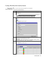
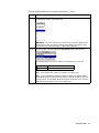
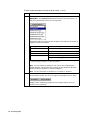
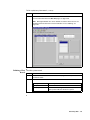
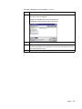
Creating a Plate Record for GeneScan Analysis . . . . . . . . . . . . . . . . . . . . . . . . . . . . . . . . . . . 3-31
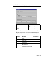
Creating a Plate Record for DNA Sequencing Analysis . . . . . . . . . . . . . . . . . . . . . . . . . . . . . 3-36
Linking and Unlinking a Plate. . . . . . . . . . . . . . . . . . . . . . . . . . . . . . . . . . . . . . . . . . . . . . . . . 3-41
Section: Running the Instrument . . . . . . . . . . . . . . . . . . . . . . . . . . . . . . . . . . . . . . .3-45
About Run Scheduling. . . . . . . . . . . . . . . . . . . . . . . . . . . . . . . . . . . . . . . . . . . . . . . . . . . . . . . 3-46
Controlling the Run . . . . . . . . . . . . . . . . . . . . . . . . . . . . . . . . . . . . . . . . . . . . . . . . . . . . . . . . . 3-47
Run Times . . . . . . . . . . . . . . . . . . . . . . . . . . . . . . . . . . . . . . . . . . . . . . . . . . . . . . . . . . . . . . . . 3-48
Section: Monitoring a Run . . . . . . . . . . . . . . . . . . . . . . . . . . . . . . . . . . . . . . . . . . . .3-49
Run View Page. . . . . . . . . . . . . . . . . . . . . . . . . . . . . . . . . . . . . . . . . . . . . . . . . . . . . . . . . . . . . 3-50
Status View Page . . . . . . . . . . . . . . . . . . . . . . . . . . . . . . . . . . . . . . . . . . . . . . . . . . . . . . . . . . . 3-51
Array View Page . . . . . . . . . . . . . . . . . . . . . . . . . . . . . . . . . . . . . . . . . . . . . . . . . . . . . . . . . . . 3-53
Capillary View Page . . . . . . . . . . . . . . . . . . . . . . . . . . . . . . . . . . . . . . . . . . . . . . . . . . . . . . . . 3-56
Instrument Status Monitor . . . . . . . . . . . . . . . . . . . . . . . . . . . . . . . . . . . . . . . . . . . . . . . . . . . . 3-57
Section: Working with Data . . . . . . . . . . . . . . . . . . . . . . . . . . . . . . . . . . . . . . . . . . .3-59
Recovering Data if Autoextraction Fails . . . . . . . . . . . . . . . . . . . . . . . . . . . . . . . . . . . . . . . . . 3-60
Viewing Raw Data from a Completed Run in the Data Collection Software . . . . . . . . . . . . . 3-61
Viewing Analyzed GeneScan Data . . . . . . . . . . . . . . . . . . . . . . . . . . . . . . . . . . . . . . . . . . . . . 3-62
Viewing Analyzed DNA Sequencing Data . . . . . . . . . . . . . . . . . . . . . . . . . . . . . . . . . . . . . . . 3-63
ii
Archiving Data . . . . . . . . . . . . . . . . . . . . . . . . . . . . . . . . . . . . . . . . . . . . . . . . . . . . . . . . . . . . 3-64
4 Spatial and Spectral Calibrations
Overview . . . . . . . . . . . . . . . . . . . . . . . . . . . . . . . . . . . . . . . . . . . . . . . . . . . . . . . . . . . . . . . . . . 4-1
Section: Spatial Calibration . . . . . . . . . . . . . . . . . . . . . . . . . . . . . . . . . . . . . . . . . . . . 4-3
About Spatial Calibrations . . . . . . . . . . . . . . . . . . . . . . . . . . . . . . . . . . . . . . . . . . . . . . . . . . . . . 4-4
About Spatial Calibration Data . . . . . . . . . . . . . . . . . . . . . . . . . . . . . . . . . . . . . . . . . . . . . . . . . 4-5
Performing a Spatial Calibration . . . . . . . . . . . . . . . . . . . . . . . . . . . . . . . . . . . . . . . . . . . . . . . . 4-6
Displaying a Spatial Calibration Profile. . . . . . . . . . . . . . . . . . . . . . . . . . . . . . . . . . . . . . . . . . 4-10
Evaluating a Spatial Calibration Profile . . . . . . . . . . . . . . . . . . . . . . . . . . . . . . . . . . . . . . . . . . 4-11
Overriding the Current Spatial Calibration Map . . . . . . . . . . . . . . . . . . . . . . . . . . . . . . . . . . . 4-12
Section: Spectral Calibration . . . . . . . . . . . . . . . . . . . . . . . . . . . . . . . . . . . . . . . . . . 4-15
About Spectral Calibrations . . . . . . . . . . . . . . . . . . . . . . . . . . . . . . . . . . . . . . . . . . . . . . . . . . . 4-16
Performing a Spectral Calibration Using Default Processing Parameters . . . . . . . . . . . . . . . . 4-18
Displaying a Spectral Calibration Profile. . . . . . . . . . . . . . . . . . . . . . . . . . . . . . . . . . . . . . . . . 4-25
Overriding a Spectral Calibration Profile. . . . . . . . . . . . . . . . . . . . . . . . . . . . . . . . . . . . . . . . . 4-28
Section: Advanced Features of Spectral Calibration . . . . . . . . . . . . . . . . . . . . . . . . 4-33
Fine-Tuning a MatrixStandard Calibration . . . . . . . . . . . . . . . . . . . . . . . . . . . . . . . . . . . . . . . 4-34
Spectral Calibration Matrices . . . . . . . . . . . . . . . . . . . . . . . . . . . . . . . . . . . . . . . . . . . . . . . . . . 4-36
Spectral Calibration Log Files . . . . . . . . . . . . . . . . . . . . . . . . . . . . . . . . . . . . . . . . . . . . . . . . . 4-37
Spectral Calibration Parameter Files . . . . . . . . . . . . . . . . . . . . . . . . . . . . . . . . . . . . . . . . . . . . 4-38
Spectral Calibration Parameters . . . . . . . . . . . . . . . . . . . . . . . . . . . . . . . . . . . . . . . . . . . . . . . . 4-40
dataType Parameter . . . . . . . . . . . . . . . . . . . . . . . . . . . . . . . . . . . . . . . . . . . . . . . . . . . . . . . . . 4-41
minQ Parameter . . . . . . . . . . . . . . . . . . . . . . . . . . . . . . . . . . . . . . . . . . . . . . . . . . . . . . . . . . . . 4-42
conditionBounds Parameter . . . . . . . . . . . . . . . . . . . . . . . . . . . . . . . . . . . . . . . . . . . . . . . . . . . 4-44
numDyes and writeDummyDyes Parameters. . . . . . . . . . . . . . . . . . . . . . . . . . . . . . . . . . . . . . 4-46
numSpectralBins Parameter . . . . . . . . . . . . . . . . . . . . . . . . . . . . . . . . . . . . . . . . . . . . . . . . . . . 4-46
Parameters Specific to sequenceStandard dataType. . . . . . . . . . . . . . . . . . . . . . . . . . . . . . . . . 4-47
startptOffset Parameter . . . . . . . . . . . . . . . . . . . . . . . . . . . . . . . . . . . . . . . . . . . . . . . . . . . . . . . 4-48
maxScansAnalyzed Parameter . . . . . . . . . . . . . . . . . . . . . . . . . . . . . . . . . . . . . . . . . . . . . . . . . 4-49
startptRange Parameter. . . . . . . . . . . . . . . . . . . . . . . . . . . . . . . . . . . . . . . . . . . . . . . . . . . . . . . 4-49
minRankQ Parameter . . . . . . . . . . . . . . . . . . . . . . . . . . . . . . . . . . . . . . . . . . . . . . . . . . . . . . . . 4-50
5 Software
Overview . . . . . . . . . . . . . . . . . . . . . . . . . . . . . . . . . . . . . . . . . . . . . . . . . . . . . . . . . . . . . . . . . . 5-1
Section: About the 3100 Software . . . . . . . . . . . . . . . . . . . . . . . . . . . . . . . . . . . . . . . 5-3
ABI PRISM 3100 Genetic Analyzer Software CD-ROMs . . . . . . . . . . . . . . . . . . . . . . . . . . . . . 5-4
3100 Genetic Analyzer Software Suite . . . . . . . . . . . . . . . . . . . . . . . . . . . . . . . . . . . . . . . . . . . 5-5
Types and Locations of Files . . . . . . . . . . . . . . . . . . . . . . . . . . . . . . . . . . . . . . . . . . . . . . . . . . . 5-9
Section: Setting the Format for the Displayed Dye Colors . . . . . . . . . . . . . . . . . . . 5-11
Using the Edit Dye Display Information Dialog Box . . . . . . . . . . . . . . . . . . . . . . . . . . . . . . . 5-12
iii
Using the Set Color Dialog Box . . . . . . . . . . . . . . . . . . . . . . . . . . . . . . . . . . . . . . . . . . . . . . . 5-13
Section: Controlling the Instrument Using Manual Control . . . . . . . . . . . . . . . . .5-15
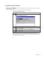
Manual Control Commands. . . . . . . . . . . . . . . . . . . . . . . . . . . . . . . . . . . . . . . . . . . . . . . . . . . 5-16
Using Manual Control Commands . . . . . . . . . . . . . . . . . . . . . . . . . . . . . . . . . . . . . . . . . . . . . 5-17
Section: Working with Run Modules . . . . . . . . . . . . . . . . . . . . . . . . . . . . . . . . . . . .5-19
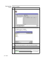
Viewing a Run Module . . . . . . . . . . . . . . . . . . . . . . . . . . . . . . . . . . . . . . . . . . . . . . . . . . . . . . 5-20
Editing or Creating a Run Module . . . . . . . . . . . . . . . . . . . . . . . . . . . . . . . . . . . . . . . . . . . . . 5-21
Run Module Parameters . . . . . . . . . . . . . . . . . . . . . . . . . . . . . . . . . . . . . . . . . . . . . . . . . . . . . 5-22
Transferring Run Modules Between Computers . . . . . . . . . . . . . . . . . . . . . . . . . . . . . . . . . . . 5-23
Section: Working with Sequencing Analysis Modules . . . . . . . . . . . . . . . . . . . . . . .5-27
Viewing and Editing Analysis Modules for DNA Sequencing . . . . . . . . . . . . . . . . . . . . . . . . 5-28
Creating a Sequencing Analysis Module. . . . . . . . . . . . . . . . . . . . . . . . . . . . . . . . . . . . . . . . . 5-30
Section: Working with GeneScan Analysis Modules . . . . . . . . . . . . . . . . . . . . . . . .5-37
Viewing and Editing Analysis Modules for GeneScan . . . . . . . . . . . . . . . . . . . . . . . . . . . . . . 5-38
Creating a GeneScan Analysis Module . . . . . . . . . . . . . . . . . . . . . . . . . . . . . . . . . . . . . . . . . . 5-40
Section: Working with BioLIMS . . . . . . . . . . . . . . . . . . . . . . . . . . . . . . . . . . . . . . . .5-47
Setting Up BioLIMS Project Information . . . . . . . . . . . . . . . . . . . . . . . . . . . . . . . . . . . . . . . . 5-48
Preparing a Plate for Extracting to BioLIMS . . . . . . . . . . . . . . . . . . . . . . . . . . . . . . . . . . . . . 5-50
After Extracting to the BioLIMS Database . . . . . . . . . . . . . . . . . . . . . . . . . . . . . . . . . . . . . . . 5-55
6 Working with Plate Records
Overview . . . . . . . . . . . . . . . . . . . . . . . . . . . . . . . . . . . . . . . . . . . . . . . . . . . . . . . . . . . . . . . . . . 6-1
Section: Introduction . . . . . . . . . . . . . . . . . . . . . . . . . . . . . . . . . . . . . . . . . . . . . . . . . .6-3
About Creating Plate Records . . . . . . . . . . . . . . . . . . . . . . . . . . . . . . . . . . . . . . . . . . . . . . . . . . 6-4
About the Plate Record Fields . . . . . . . . . . . . . . . . . . . . . . . . . . . . . . . . . . . . . . . . . . . . . . . . . . 6-5
Section: Tab-Delimited Text Files . . . . . . . . . . . . . . . . . . . . . . . . . . . . . . . . . . . . . . . .6-9
Introduction to Tab-Delimited Text Files . . . . . . . . . . . . . . . . . . . . . . . . . . . . . . . . . . . . . . . . 6-10
About Creating Tab-Delimited Text Files . . . . . . . . . . . . . . . . . . . . . . . . . . . . . . . . . . . . . . . . 6-11
Using Spreadsheets to Create Tab-Delimited Text Files . . . . . . . . . . . . . . . . . . . . . . . . . . . . . 6-12
Spreadsheet or Tab-Delimited Text File Information . . . . . . . . . . . . . . . . . . . . . . . . . . . . . . . 6-14
Running the Same Sample with Different Conditions . . . . . . . . . . . . . . . . . . . . . . . . . . . . . . 6-18
Section: Creating a Plate Record by Importing LIMS Data . . . . . . . . . . . . . . . . . .6-19
Data Transfer . . . . . . . . . . . . . . . . . . . . . . . . . . . . . . . . . . . . . . . . . . . . . . . . . . . . . . . . . . . . . . 6-20
Plate Import Table . . . . . . . . . . . . . . . . . . . . . . . . . . . . . . . . . . . . . . . . . . . . . . . . . . . . . . . . . . 6-21
Section: Creating Plate Files . . . . . . . . . . . . . . . . . . . . . . . . . . . . . . . . . . . . . . . . . . .6-23
Creating a Plate File Using a Provided Template . . . . . . . . . . . . . . . . . . . . . . . . . . . . . . . . . . 6-24
Creating a Plate File from a New Spreadsheet . . . . . . . . . . . . . . . . . . . . . . . . . . . . . . . . . . . . 6-28
Creating a Plate File from a Custom Spreadsheet Template . . . . . . . . . . . . . . . . . . . . . . . . . . 6-29
Creating a Plate File from an Edited Plate Record . . . . . . . . . . . . . . . . . . . . . . . . . . . . . . . . . 6-30
Section: Importing Plate Files and Linking Plate Records . . . . . . . . . . . . . . . . . . .6-31
About Importing Tab-Delimited Text Files and Linking Plate Records . . . . . . . . . . . . . . . . . 6-32
Simultaneously Importing and Linking a Plate Record. . . . . . . . . . . . . . . . . . . . . . . . . . . . . . 6-33
iv
Sequentially Importing and Linking a Plate Record . . . . . . . . . . . . . . . . . . . . . . . . . . . . . . . . 6-35
Section: Deleting Plate Records and Run Data . . . . . . . . . . . . . . . . . . . . . . . . . . . . 6-37
Introduction . . . . . . . . . . . . . . . . . . . . . . . . . . . . . . . . . . . . . . . . . . . . . . . . . . . . . . . . . . . . . . . 6-38
Cleanup Database Utility . . . . . . . . . . . . . . . . . . . . . . . . . . . . . . . . . . . . . . . . . . . . . . . . . . . . . 6-38
Deleting Individual Plate Records . . . . . . . . . . . . . . . . . . . . . . . . . . . . . . . . . . . . . . . . . . . . . . 6-39
7 System Management and Networking
Overview . . . . . . . . . . . . . . . . . . . . . . . . . . . . . . . . . . . . . . . . . . . . . . . . . . . . . . . . . . . . . . . . . . 7-1
Section: Managing Hard Drive and Instrument Database Space . . . . . . . . . . . . . . 7-3
How Run Data Is Stored. . . . . . . . . . . . . . . . . . . . . . . . . . . . . . . . . . . . . . . . . . . . . . . . . . . . . . . 7-4
Checking Database Space: The Diskspace Utility . . . . . . . . . . . . . . . . . . . . . . . . . . . . . . . . . . . 7-5
Re-Extracting Processed Frame Data: The Re-Extraction Utility . . . . . . . . . . . . . . . . . . . . . . . 7-6
Deleting Processed Frame Data: The Cleanup Database Utility . . . . . . . . . . . . . . . . . . . . . . . . 7-8
Importing a New Spatial or Spectral Calibration Method:
The New Method Import Utility. . . . . . . . . . . . . . . . . . . . . . . . . . . . . . . . . . . . . . . . . . . . . . . . 7-10
Removing Run Modules from the Instrument Database:
The Remove Run Modules Utility . . . . . . . . . . . . . . . . . . . . . . . . . . . . . . . . . . . . . . . . . . . . . . 7-11
Reinitializing the Instrument Database: The Initialize Database Utility . . . . . . . . . . . . . . . . . 7-12
Section: Networking . . . . . . . . . . . . . . . . . . . . . . . . . . . . . . . . . . . . . . . . . . . . . . . . . 7-13
Networking Options . . . . . . . . . . . . . . . . . . . . . . . . . . . . . . . . . . . . . . . . . . . . . . . . . . . . . . . . . 7-14
Networking the Computer Workstation . . . . . . . . . . . . . . . . . . . . . . . . . . . . . . . . . . . . . . . . . . 7-16
Requirements for a Networked Computer . . . . . . . . . . . . . . . . . . . . . . . . . . . . . . . . . . . . . . . . 7-18
8 Maintenance
Overview . . . . . . . . . . . . . . . . . . . . . . . . . . . . . . . . . . . . . . . . . . . . . . . . . . . . . . . . . . . . . . . . . . 8-1
Section: Instrument Maintenance . . . . . . . . . . . . . . . . . . . . . . . . . . . . . . . . . . . . . . . 8-3
Maintenance Task Lists . . . . . . . . . . . . . . . . . . . . . . . . . . . . . . . . . . . . . . . . . . . . . . . . . . . . . . . 8-4
Routine Cleaning . . . . . . . . . . . . . . . . . . . . . . . . . . . . . . . . . . . . . . . . . . . . . . . . . . . . . . . . . . . . 8-5
Moving and Leveling the Instrument . . . . . . . . . . . . . . . . . . . . . . . . . . . . . . . . . . . . . . . . . . . . . 8-6
Resetting the Instrument. . . . . . . . . . . . . . . . . . . . . . . . . . . . . . . . . . . . . . . . . . . . . . . . . . . . . . . 8-7
Shutting Down the Instrument . . . . . . . . . . . . . . . . . . . . . . . . . . . . . . . . . . . . . . . . . . . . . . . . . . 8-8
Section: Fluids and Waste . . . . . . . . . . . . . . . . . . . . . . . . . . . . . . . . . . . . . . . . . . . . . 8-9
Buffer . . . . . . . . . . . . . . . . . . . . . . . . . . . . . . . . . . . . . . . . . . . . . . . . . . . . . . . . . . . . . . . . . . . . 8-10
Polymer. . . . . . . . . . . . . . . . . . . . . . . . . . . . . . . . . . . . . . . . . . . . . . . . . . . . . . . . . . . . . . . . . . . 8-10
Handling Instrument Waste . . . . . . . . . . . . . . . . . . . . . . . . . . . . . . . . . . . . . . . . . . . . . . . . . . . 8-12
Section: Capillary Array . . . . . . . . . . . . . . . . . . . . . . . . . . . . . . . . . . . . . . . . . . . . . . 8-13
Before Installing a Previously Used Capillary Array. . . . . . . . . . . . . . . . . . . . . . . . . . . . . . . . 8-14
Installing and Removing the Capillary Array . . . . . . . . . . . . . . . . . . . . . . . . . . . . . . . . . . . . . 8-15
Capillary Array Maintenance . . . . . . . . . . . . . . . . . . . . . . . . . . . . . . . . . . . . . . . . . . . . . . . . . . 8-16
Storing a Capillary Array on the Instrument . . . . . . . . . . . . . . . . . . . . . . . . . . . . . . . . . . . . . . 8-17
Storing a Capillary Array off the Instrument . . . . . . . . . . . . . . . . . . . . . . . . . . . . . . . . . . . . . . 8-17
v
Section: Syringes . . . . . . . . . . . . . . . . . . . . . . . . . . . . . . . . . . . . . . . . . . . . . . . . . . . .8-19
Syringe Maintenance . . . . . . . . . . . . . . . . . . . . . . . . . . . . . . . . . . . . . . . . . . . . . . . . . . . . . . . . 8-20
Cleaning and Inspecting Syringes . . . . . . . . . . . . . . . . . . . . . . . . . . . . . . . . . . . . . . . . . . . . . . 8-21
Priming and Filling Syringes . . . . . . . . . . . . . . . . . . . . . . . . . . . . . . . . . . . . . . . . . . . . . . . . . . 8-22
Installing and Removing Syringes. . . . . . . . . . . . . . . . . . . . . . . . . . . . . . . . . . . . . . . . . . . . . . 8-23
Section: Polymer Blocks . . . . . . . . . . . . . . . . . . . . . . . . . . . . . . . . . . . . . . . . . . . . . .8-25
Removing the Polymer Blocks . . . . . . . . . . . . . . . . . . . . . . . . . . . . . . . . . . . . . . . . . . . . . . . . 8-26
Cleaning the Polymer Blocks . . . . . . . . . . . . . . . . . . . . . . . . . . . . . . . . . . . . . . . . . . . . . . . . . 8-27
Removing Air Bubbles from the Upper Polymer Block . . . . . . . . . . . . . . . . . . . . . . . . . . . . . 8-28
Section: Autosampler Calibration . . . . . . . . . . . . . . . . . . . . . . . . . . . . . . . . . . . . . . .8-29
9 Troubleshooting
Overview . . . . . . . . . . . . . . . . . . . . . . . . . . . . . . . . . . . . . . . . . . . . . . . . . . . . . . . . . . . . . . . . . . 9-1
Instrument Startup . . . . . . . . . . . . . . . . . . . . . . . . . . . . . . . . . . . . . . . . . . . . . . . . . . . . . . . . . . . 9-2
Spatial Calibration . . . . . . . . . . . . . . . . . . . . . . . . . . . . . . . . . . . . . . . . . . . . . . . . . . . . . . . . . . . 9-3
Spectral Calibration . . . . . . . . . . . . . . . . . . . . . . . . . . . . . . . . . . . . . . . . . . . . . . . . . . . . . . . . . . 9-4
Run Performance . . . . . . . . . . . . . . . . . . . . . . . . . . . . . . . . . . . . . . . . . . . . . . . . . . . . . . . . . . . . 9-5
A Data Flow
Overview . . . . . . . . . . . . . . . . . . . . . . . . . . . . . . . . . . . . . . . . . . . . . . . . . . . . . . . . . . . . . . . . . . A-1
About Data Flow . . . . . . . . . . . . . . . . . . . . . . . . . . . . . . . . . . . . . . . . . . . . . . . . . . . . . . . . . . . . A-2
Organization of the CCD . . . . . . . . . . . . . . . . . . . . . . . . . . . . . . . . . . . . . . . . . . . . . . . . . . . . . . A-3
Incident Fluorescence . . . . . . . . . . . . . . . . . . . . . . . . . . . . . . . . . . . . . . . . . . . . . . . . . . . . . . . . A-4
Frame Data . . . . . . . . . . . . . . . . . . . . . . . . . . . . . . . . . . . . . . . . . . . . . . . . . . . . . . . . . . . . . . . . A-5
Multicomponenting . . . . . . . . . . . . . . . . . . . . . . . . . . . . . . . . . . . . . . . . . . . . . . . . . . . . . . . . . . A-6
Configuring Data Flow . . . . . . . . . . . . . . . . . . . . . . . . . . . . . . . . . . . . . . . . . . . . . . . . . . . . . . . A-7
Mobility Shift Correction for DNA Sequencing . . . . . . . . . . . . . . . . . . . . . . . . . . . . . . . . . . . . A-8
B Technical Support
Technical Support . . . . . . . . . . . . . . . . . . . . . . . . . . . . . . . . . . . . . . . . . . . . . . . . . . . . . . . . . . . B-1
C Part Numbers
Applied Biosystems Part Numbers . . . . . . . . . . . . . . . . . . . . . . . . . . . . . . . . . . . . . . . . . . . . . . C-1
D Limited Warranty Statement
vi
Introduction and Safety 1
1
Overview
In This Chapter The following topics are covered in this chapter:
Topic
See Page
ABI PRISM 3100 Genetic Analyzer
1-2
To Get Started Quickly
1-3
Additional Documentation
1-4
Safety
1-5
Introduction and Safety 1-1
ABI PRISM 3100 Genetic Analyzer
Definition The ABI PRISM ® 3100 Genetic Analyzer is an automated capillary electrophoresis
system that can separate, detect, and analyze up to 16 capillaries of fluorescently
labeled DNA fragments in one run.
System Components The 3100 Genetic Analyzer system includes the following components:
1-2 Introduction and Safety
♦
ABI PRISM ® 3100 Genetic Analyzer
♦
Computer workstation with Microsoft® Windows® NT operating system
♦
ABI PRISM ® 3100 Genetic Analyzer software
♦
ABI PRISM ® DNA Sequencing Analysis or ABI PRISM ® GeneScan® Analysis
software
♦
Capillary array
♦
Reagent consumables
To Get Started Quickly
Important Safety Before using the 3100 Genetic Analyzer, read the safety information starting on page
Information 1-5 and in the ABI PRISM 3100 Genetic Analyzer Site Preparation and Safety Guide
(P/N 4315835).
What You Should This manual is written for principle investigators and laboratory staff who are planning
Know to operate and maintain a 3100 Genetic Analyzer.
Before attempting the procedures in this manual, you should be familiar with the
following topics:
♦
Windows NT operating system
♦
General techniques for handling DNA samples and preparing them for
electrophoresis. Detailed information about preparing samples for sequencing
and fragment analysis is given in other Applied Biosystems’ manuals (see the
table below).
♦
Networking, which is needed if you want to integrate the 3100 Genetic Analyzer
into your existing laboratory data flow system
Getting Started The following table lists the sources of specific information to help you get started
Quickly quickly:
For instruction on how to...
Refer to...
♦ prepare DNA templates
ABI PRISM 3100 Genetic Analyzer
Sequencing Chemistry Guide (P/N 4315831)
♦ perform cycle sequencing
♦ prepare extension products
♦ prepare samples for sequencing
analysis
ABI PRISM 3100 Genetic Analyzer Quick Start
Guide for Sequencing (P/N 4315833)
♦ perform a sequencing analysis run and
view run data
♦ prepare samples for fragment analysis
♦ perform a fragment analysis run and
view run data
ABI PRISM 3100 Genetic Analyzer Quick Start
Guide for Fragment Analysis (P/N 4315832)
calibrate this instrument
Chapter 4, “Spatial and Spectral Calibrations.”
operate this instrument (detailed)
Chapter 3, “Performing a Run.”
Introduction and Safety 1-3
Additional Documentation
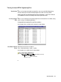
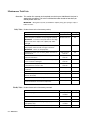
List of User The following table lists the complete ABI PRISM 3100 Genetic Analyzer document set
Documents for users:
Title
Contents
ABI PRISM 3100 Genetic Analyzer
Site Preparation and Safety Guide
♦ Laboratory requirements for
installation
P/N
Instrument
4315835
♦ Instrument and chemical safety
ABI PRISM 3100 Genetic Analyzer
User’s Manual
♦ User procedures
4315834
♦ Instrument maintenance
♦ Troubleshooting
ABI PRISM 3100 Genetic Analyzer
Quick Start Guide for Fragment
Analysis
Abbreviated procedures for performing a
fragment analysis run
4315832
ABI PRISM 3100 Genetic Analyzer
Quick Start Guide for Sequencing
Abbreviated procedures for performing a
sequencing run
4315833
Software
ABI PRISM DNA Sequencing
Analysis Software v. 3.6 NT User’s
Manual
Detailed procedures for analyzing
sequencing data
4308924
Detailed procedures for analyzing
fragment analysis data
4308923
ABI PRISM DNA Sequencing
Analysis Software Release Notes
ABI PRISM GeneScan Analysis
Software v. 3.5 NT User’s Manual
ABI PRISM GeneScan Analysis
Software Release Notes
Chemistry
ABI PRISM 3100 Genetic Analyzer
Sequencing Chemistry Guide
♦ Detailed chemistry procedures
specific for the 3100 Genetic Analyzer
4315831
♦ Chemistry troubleshooting for the
3100 Genetic Analyzer
ABI PRISM Automated DNA
Sequencing Chemistry Guide
♦ A description of DNA sequencing
instruments, chemistries, and software
4305080
♦ Detailed procedures for preparing
DNA templates, performing cycle
sequencing, and preparing extension
products
About User Bulletins User bulletins are the mechanism we use to inform our customers of technical
information, product improvements, and related new products and laboratory
techniques.
User bulletins related to the use of this instrument will be mailed to you. We
recommend storing the bulletins in this manual. A tab labeled “User Bulletins” has
been included for this purpose.
1-4 Introduction and Safety
Safety
Documentation User Five user attention words appear in the text of all Applied Biosystems user
Attention Words documentation. Each word implies a particular level of observation or action as
described below.
Note
Calls attention to useful information.
IMPORTANT Indicates information that is necessary for proper instrument operation.
! CAUTION Indicates a potentially hazardous situation which, if not avoided, may result in
minor or moderate injury. It may also be used to alert against unsafe practices.
! WARNING Indicates a potentially hazardous situation which, if not avoided, could result in
death or serious injury.
! DANGER Indicates an imminently hazardous situation which, if not avoided, will result in
death or serious injury. This signal word is to be limited to the most extreme situations.
Chemical Hazard ! WARNING CHEMICAL HAZARD. Some of the chemicals used with Applied Biosystems
Warning instruments and protocols are potentially hazardous and can cause injury, illness, or death.
♦
Read and understand the material safety data sheets (MSDSs) provided by the
chemical manufacturer before you store, handle, or work with any chemicals or
hazardous materials.
♦
Minimize contact with and inhalation of chemicals. Wear appropriate personal
protective equipment when handling chemicals (e.g., safety glasses, gloves, or
protective clothing). For additional safety guidelines, consult the MSDS.
♦
Do not leave chemical containers open. Use only with adequate ventilation.
♦
Check regularly for chemical leaks or spills. If a leak or spill occurs, follow the
manufacturer’s cleanup procedures as recommended on the MSDS.
♦
Comply with all local, state/provincial, or national laws and regulations related to
chemical storage, handling, and disposal.
\
Chemical Waste ! WARNING CHEMICAL WASTE HAZARD. Wastes produced by Applied Biosystems
Hazard Warning instruments are potentially hazardous and can cause injury, illness, or death.
♦
Read and understand the material safety data sheets (MSDSs) provided by the
manufacturers of the chemicals in the waste container before you store, handle, or
dispose of chemical waste.
♦
Handle chemical wastes in a fume hood.
♦
Minimize contact with and inhalation of chemical waste. Wear appropriate
personal protective equipment when handling chemicals (e.g., safety glasses,
gloves, or protective clothing).
♦
After emptying the waste container, seal it with the cap provided.
♦
Dispose of the contents of the waste tray and waste bottle in accordance with
good laboratory practices and local, state/provincial, or national environmental
and health regulations.
Site Preparation and A site preparation and safety guide is a separate document sent to all customers who
Safety Guide have purchased an Applied Biosystems instrument. Refer to the guide written for your
Introduction and Safety 1-5
instrument for information on site preparation, instrument safety, chemical safety, and
waste profiles.
About MSDSs Some of the chemicals used with this instrument may be listed as hazardous by their
manufacturer. When hazards exist, warnings are prominently displayed on the labels
of all chemicals.
Chemical manufacturers supply a current MSDS before or with shipments of
hazardous chemicals to new customers and with the first shipment of a hazardous
chemical after an MSDS update. MSDSs provide you with the safety information you
need to store, handle, transport and dispose of the chemicals safely.
We strongly recommend that you replace the appropriate MSDS in your files each
time you receive a new MSDS packaged with a hazardous chemical.
! WARNING CHEMICAL HAZARD. Be sure to familiarize yourself with the MSDSs
before using reagents or solvents.
Ordering MSDSs You can order free additional copies of MSDSs for chemicals manufactured or
distributed by Applied Biosystems using the contact information below.
To order MSDSs...
Over the Internet
Then...
a. Go to our Web site at www.appliedbiosystems.com/techsupp
b. Click MSDSs
If you have...
Then...
The MSDS document
number or the Document
on Demand index number
Enter one of these
numbers in the appropriate
field on this page.
The product part number
Select Click Here, then
enter the part number or
keyword(s) in the field on
this page.
Keyword(s)
c. You can open and download a PDF (using Adobe® Acrobat®
Reader™) of the document by selecting it, or you can choose
to have the document sent to you by fax or email.
By automated telephone
service
Use “To Obtain Documents on Demand” under “Technical
Support.”
By telephone in the
United States
Dial 1-800-327-3002, then press 1.
By telephone from
Canada
By telephone from any
other country
To order in...
Dial 1-800-668-6913 and...
English
Press 1, then 2, then 1 again
French
Press 2, then 2, then 1
See the specific region under “To Contact Technical Support by
Telephone or Fax” under “Technical Support.”
For chemicals not manufactured or distributed by Applied Biosystems, call the
chemical manufacturer.
1-6 Introduction and Safety
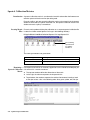
Instrument Safety Safety labels are located on the instrument. Each safety label has three parts:
Labels ♦ A signal word panel, which implies a particular level of observation or action (e.g.,
CAUTION or WARNING). If a safety label encompasses multiple hazards, the
signal word corresponding to the greatest hazard is used.
♦
A message panel, which explains the hazard and any user action required.
♦
A safety alert symbol, which indicates a potential personal safety hazard. See the
ABI Prism 3100 Genetic Analyzer Site Preparation and Safety Guide for an
explanation of all the safety alert symbols provided in several languages.
About Waste As the generator of potentially hazardous waste, it is your responsibility to perform the
Disposal actions listed below.
♦
Characterize (by analysis if necessary) the waste generated by the particular
applications, reagents, and substrates used in your laboratory.
♦
Ensure the health and safety of all personnel in your laboratory.
♦
Ensure that the instrument waste is stored, transferred, transported, and disposed
of according to all local, state/provincial, or national regulations.
Note Radioactive or biohazardous materials may require special handling, and disposal
limitations may apply.
Before Operating the Ensure that everyone involved with the operation of the instrument has:
Instrument ♦ Received instruction in general safety practices for laboratories
♦
Received instruction in specific safety practices for the instrument
♦
Read and understood all related MSDSs
! CAUTION Avoid using this instrument in a manner not specified by Applied Biosystems.
Although the instrument has been designed to protect the user, this protection can be impaired
if the instrument is used improperly.
Safe and Efficient Operating the computer correctly prevents stress-producing effects such as fatigue,
Computer Use pain, and strain.
To minimize these effects on your back, legs, eyes, and upper extremities (neck,
shoulder, arms, wrists, hands and fingers), design your workstation to promote neutral
or relaxed working positions. This includes working in an environment where heating,
air conditioning, ventilation, and lighting are set correctly. See the guidelines below.
! CAUTION MUSCULOSKELETAL AND REPETITIVE MOTION HAZARD. These hazards
are caused by the following potential risk factors which include, but are not limited to, repetitive
motion, awkward posture, forceful exertion, holding static unhealthy positions, contact pressure,
and other workstation environmental factors.
♦
Use a seating position that provides the optimum combination of comfort,
accessibility to the keyboard, and freedom from fatigue-causing stresses and
pressures.
–
The bulk of the person’s weight should be supported by the buttocks, not the
thighs.
–
Feet should be flat on the floor, and the weight of the legs should be
supported by the floor, not the thighs.
Introduction and Safety 1-7
–
♦
Lumbar support should be provided to maintain the proper concave curve of
the spine.
Place the keyboard on a surface that provides:
–
The proper height to position the forearms horizontally and upper arms
vertically.
–
Support for the forearms and hands to avoid muscle fatigue in the upper arms.
♦
Position the viewing screen to the height that allows normal body and head
posture. This height depends upon the physical proportions of the user.
♦
Adjust vision factors to optimize comfort and efficiency by:
♦
–
Adjusting screen variables, such as brightness, contrast, and color, to suit
personal preferences and ambient lighting.
–
Positioning the screen to minimize reflections from ambient light sources.
–
Positioning the screen at a distance that takes into account user variables
such as nearsightedness, farsightedness, astigmatism, and the effects of
corrective lenses.
When considering the user’s distance from the screen, the following are useful
guidelines:
–
The distance from the user’s eyes to the viewing screen should be
approximately the same as the distance from the user’s eyes to the keyboard.
–
For most people, the reading distance that is the most comfortable is
approximately 20 inches.
–
The workstation surface should have a minimum depth of 36 inches to
accommodate distance adjustment.
–
Adjust the screen angle to minimize reflection and glare, and avoid highly
reflective surfaces for the workstation.
♦
Use a well-designed copy holder, adjustable horizontally and vertically, that allows
referenced hard-copy material to be placed at the same viewing distance as the
screen and keyboard.
♦
Keep wires and cables out of the way of users and passersby.
♦
Choose a workstation that has a surface large enough for other tasks and that
provides sufficient legroom for adequate movement.
Electric Shock
! WARNING ELECTRICAL SHOCK HAZARD. To reduce the chance of electrical shock, do
not remove covers that require tool access. No user serviceable parts are inside. Refer
servicing to Applied Biosystems qualified service personnel.
Lifting/Moving
! WARNING PHYSICAL INJURY HAZARD. Do not attempt to lift the instrument or any
other heavy objects unless you have received related training. Incorrect lifting can cause painful
and sometimes permanent back injury. Use proper lifting techniques when lifting or moving the
instrument. Two or three people are required to lift the instrument, depending upon instrument
weight.
1-8 Introduction and Safety
System Overview
2
2
Overview
In This Chapter The following topics are covered in this chapter:
Topic
See Page
Section: 3100 Instrument Overview
2-3
ABI PRISM 3100 System Components
2-4
What the Instrument Does
2-5
How the Instrument Works
2-6
Section: Instrument Hardware Overview
2-9
Front View
2-10
Front View with Doors Open
2-11
Back View
2-12
Section: Computer and Software Overview
2-13
Computer Workstation
2-14
Software
2-15
Section: Chemistry Overview
2-17
Supported Dye Sets
2-18
Labeling Chemistries
2-19
Polymers
2-20
Injection Solution
2-21
Section: Electrophoresis Overview
2-23
Capillary Array
2-24
Electrophoresis
2-25
Electrophoresis Circuit
2-26
Section: Fluorescence Detection Overview
2-27
Introduction
2-28
Laser
2-29
Transmission Grating
2-29
CCD Camera
2-29
System Overview 2-1
2-2 System Overview
Section: 3100 Instrument Overview
In This Section The following topics are covered in this section:
Topic
See Page
ABI PRISM 3100 System Components
2-4
What the Instrument Does
2-5
How the Instrument Works
2-6
System Overview 2-3
ABI PRISM 3100 System Components
Table of The ABI PRISM ® 3100 Genetic Analyzer system includes the following components:
Components
Component
For detailed information, see...
ABI PRISM 3100 Genetic
Analyzer
♦ “What the Instrument Does” on page 2-5.
♦ “How the Instrument Works” on page 2-6.
♦ “Instrument Hardware Overview” on page 2-9.
Computer workstation with
Microsoft® Windows® NT
operating system
ABI PRISM 3100 Genetic
Analyzer software
♦ “Computer Workstation” on page 2-14.
♦ “Managing Hard Drive and Instrument Database
Space” on page 7-3.
♦ “Software” on page 2-15.
♦ Chapter 5, “Software.”
ABI
DNA Sequencing
Analysis or GeneScan®
Analysis software
♦ ABI PRISM DNA Sequencing Analysis Software v. 3.6
NT User’s Manual (P/N 4308924).
Capillary Array
♦ “Capillary Array” on page 2-24.
PRISM ®
♦ ABI PRISM GeneScan Analysis Software v. 3.5 NT
User’s Manual (P/N 4308923).
♦ Appendix C, “Part Numbers.”
Reagent consumables
♦ “Polymers” on page 2-20.
♦ “Injection Solution” on page 2-21.
♦ Appendix C, “Part Numbers.”
2-4 System Overview
What the Instrument Does
Types of Analysis The 3100 Genetic Analyzer performs two kinds of analysis:
DNA Analysis
Purpose
Sequencing analysis
♦ Separates a mixture of DNA fragments according to their
lengths
♦ Provides a profile of the separation
♦ Determines the order of the four deoxyribonucleotide bases
Fragment analysis
♦ Separates a mixture of DNA fragments according to their
lengths
♦ Provides a profile of the separation
♦ Determines the length of each fragment (in basepairs)
♦ Estimates the relative concentration of each fragment in the
sample
System Overview 2-5
How the Instrument Works
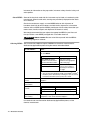
Description of a The following table describes a typical run on the 3100 instrument:
Typical Run
Stage
1
Description
Sample Preparation
During sample preparation, the DNA fragments in a sample are
chemically labeled with fluorescent dyes.
The dyes facilitate the detection and identification of the DNA.
Typically, each DNA molecule is labeled with one dye molecule,
but up to five dyes can be used to label the DNA sample.
Both the type of fluorescent labeling and the sample
composition vary with the sample preparation method used.
Samples are prepared in 96- or 384-well plates.
2
Software Setup
The operator creates a plate record and specifies the sample
type and run module in the ABI PRISM ® 3100 Data Collection
software.
3
Beginning the Run
The operator places the plates on the instrument and starts the
run.
The autosampler automatically moves the sample plate into
position to be sampled by the 16 capillaries.
4
Electrophoresis
Molecules from the samples are electrophoretically injected into
thin, fused-silica capillaries that have been filled with polymer.
Electrophoresis of all samples begins at the same time when a
voltage is applied across all capillaries.
The DNA fragments migrate towards the other end of the
capillaries, with the shorter fragments moving faster than the
longer fragments.
5
Excitation and Detection
As the fragments enter the detection cell, they move through the
path of a laser beam. The laser light causes the dye on the
fragments to fluoresce.
The fluorescence is captured by a charge-coupled device (CCD)
camera.
2-6 System Overview
Diagram
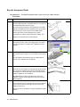
Stage
6
Description
Diagram
Data Collection
The CCD camera converts the fluorescence information into
electronic information, which is then transferred to the computer
workstation for processing by the 3100 Data Collection software.
7
Data Processing
After the data is processed, it is stored in the instrument
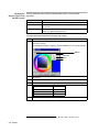
database and displayed as an electropherogram.
An electropherogram plots relative dye concentration (y-axis)
against time (x-axis) for each of the dyes used to label the DNA
fragments.
Each peak in the electropherogram represents a single
fragment.
8
Automatic Data Extraction and Data Analysis
The processed data is automatically extracted from the
instrument database and analyzed.
The positions and shapes of the electropherogram peaks are
used to determine either the base sequence or fragment profile,
depending on the type of run selected.
The analyzed data is stored as sample files on the hard drive of
the computer.
9
Viewing the Results
The analyzed data is viewed with either DNA Sequencing
Analysis software (for sequencing) or GeneScan Analysis
software (for fragment analysis).
If necessary, the data is reanalyzed using different analysis
parameters.
System Overview 2-7
2-8 System Overview
Section: Instrument Hardware Overview
In This Section The following topics are covered in this section:
Topic
See Page
Front View
2-10
Front View with Doors Open
2-11
Back View
2-12
System Overview 2-9
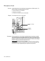
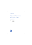
Front View
Diagram The following diagram shows the front of the instrument:
Doors
Light switch
Tray button
Reset button
Status lights
On/Off button
Description
Part
Function
Light switch
Switches on and off the interior lights
On/Off button
Switches on and off the instrument
Reset button
Resets all of the electronics on the instrument including the
firmware and the calibration file
IMPORTANT Use this button only as a last resort when the
instrument is not responding. See page 8-7 for procedure.
Tray button
Brings the autosampler to the forward position
Note This button works only when the instrument and
oven doors are closed.
Status lights
Indicates the status of the instrument as follows:
Light Appearance
Instrument Status
All off
Power off
Yellow solid
Loading firmware
Yellow blinking
♦ Loading calibration file
Green solid
Ready for use
Green blinking
Running
Red blinking
Error
♦ Initializing subsystems
2-10 System Overview
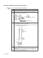
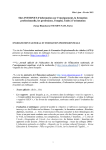
Front View with Doors Open
Diagram The following diagram shows inside the instrument’s doors:
Polymer-reserve syringe
Upper polymer
block
Array-fill syringe
Oven
Detection cell
Capillary array
Buffer and water
reservoirs
Autosampler
Lower polymer block
Anode buffer reservoir
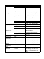
Description
Part
Function
Anode buffer reservoir
Contains 9-mL of 1X running buffer
Buffer and water
reservoirs (four)
Contains 16-mL of 1X running buffer or water
Autosampler
Holds the sample plates and reservoirs and moves to align the
samples, water, or buffer with the capillaries.
Capillary array
Enable the separation of the fluorescently labeled DNA
fragments by electrophoresis. It is a replaceable unit composed
of 16 silica capillaries.
Detection cell
Holds the capillaries in place for laser detection
Lower polymer block
Contains the anode electrode. The anode buffer reservoir
connects to this block.
Oven
Maintains uniform capillary array temperature
Polymer-reserve syringe
Contains and dispenses the polymer that fills the polymer
blocks and the array-fill syringe. A 5-mL syringe.
Array-fill syringe
Contains and dispenses the polymer under high pressure to fill
the capillaries. A 250-µL syringe.
Upper polymer block
Connects the two syringes and the detection end of the
capillary array
System Overview 2-11
Back View
Diagram The following diagram shows the back of the instrument:
Chassis fan
Laser fan
Ethernet outlet
Power cord
Air filter holder
Air inlet vents
Description
Part
Function
Air filter holder
Holds the filter that cleans the air entering the instrument
Air inlet vents
Allows air into instrument
IMPORTANT To ensure adequate air flow, do not place
paper under the instrument.
2-12 System Overview
Ethernet outlet
Provides a network connection to the computer workstation
Chassis fan
Pulls air out of the instrument
Laser fan
Cools the laser
Power cord
Supplies power to the instrument
Section: Computer and Software Overview
In This Section The following topics are covered in this section:
Topic
See Page
Computer Workstation
2-14
Software
2-15
System Overview 2-13
Computer Workstation
Overview The 3100 Genetic Analyzer is shipped with a computer workstation running the
Microsoft Windows NT operating system. An optional color printer is available.
This manual is written with the assumption that you know how to use a computer
workstation running the Windows NT operating system. If you are not familiar with this
computer, refer to the Windows NT workstation documentation shipped with this
system for specific operating information.
Function The computer workstation collects and analyzes data from the 3100 Genetic Analyzer.
System The following table lists the minimum requirements for the computer workstation:
Requirements
Item
Minimum Requirements
Hard drive storage
2 drives, 9 GB each
Memory
256 MB RAM
Monitor
17-in. SVGA
Operating system
Microsoft® Windows® NT v. 4.0 with Service Pack 5
Printer
Optional
Processor
Intel Pentium III 550 MHz
Hard Drive During installation, the hard drives of your computer workstation were partitioned to
Partitions create the following logical drives:
Physical Hard
Disk
Drive
Size
(GB)
1
C
2
Function
System operating files
Note You may also install your own programs on this
drive.
2
2-14 System Overview
D
7
Reserved for the 3100 software and the analysis
software
E
9
Reserved for the instrument database
Software
Overview The software installed on your computer workstation consists of:
♦
Data Collection software that controls, monitors, and collects data from the
instrument
♦
An analysis application that either analyzes raw sequencing data or sizes and
quantifies DNA fragments
♦
Software that automatically extracts and analyzes the data
♦
A database
♦
Utilities that enable you to manage the files in the database
♦
A toolkit that enables you to develop customized applications
For a complete list of the ABI PRISM 3100 software installed on your computer, see
page 5-5.
Note Other programs are available from Applied Biosystems to align sequences, identify
previously unsequenced regions, archive data, identify patterns of heredity, and perform other
kinds of data manipulation. See your Applied Biosystems representative.
Note To avoid software conflicts, it is recommended that you do not install third-party software
onto the computer attached to the 3100 instrument.
System Overview 2-15
2-16 System Overview
Section: Chemistry Overview
In This Section The following topics are covered in this section:
Topic
See Page
Supported Dye Sets
2-18
Labeling Chemistries
2-19
Polymers
2-20
Injection Solution
2-21
Overview This section provides an overview of the chemistry. For more detailed information, see
the ABI PRISM 3100 Genetic Analyzer Sequencing Chemistry Guide.
System Overview 2-17
Supported Dye Sets
Overview DNA fragments are detected and identified by the fluorescent dyes with which they are
chemically labeled. Dyes are purchased and used as dye sets, which are optimized for
particular applications.
Table of Supported Two dye sets are currently supported by Applied Biosystems for use with the
Dye Sets 3100 Genetic Analyzer.
Note Other dye sets can also be used for sequencing with the 3100 Genetic Analyzer (see
“dataType Parameter” on page 4-41).
Dye Set
D
Comprises...
Use for...
♦ 6FAM™
Fragment analysis
♦ HEX™
♦ NED™
♦ ROX™
E
dRhodamine and ABI PRISM ® BigDye™
versions of:
DNA sequencing
♦ dROX™
♦ dTAMRA™
♦ dR6G
♦ dR110
Ea
SNP Detection Snapshot
a. The ABI PRISM ® BigDyeTM dye set has a similar spectral profile as Dye Set E. Customers have
successfully used Dye Set E matrix standards for BigDye dyes. For best performance, however, we
recommend that you create the matrix from Long-Read standards.
2-18 System Overview
Labeling Chemistries
Supported Labeling The 3100 Genetic Analyzer is currently supported by Applied Biosystems for use with:
Chemistries ♦ DNA sequencing samples that are fluorescently labeled with:
–
ABI PRISM ® BigDye™ Terminator Cycle Sequencing Ready Reaction Kit
–
ABI PRISM ® BigDye™ Primer Cycle Sequencing Ready Reaction Kit
–
ABI PRISM™ dRhodamine Terminator Cycle Sequencing Ready Reaction Kit
Note
♦
These chemistries use the dyes in Dye Set E.
Fragment analysis samples that are labeled with the fluorescent primers supplied
with the ABI PRISM ® Linkage Mapping Set-LD20, MD10, or HD5.
Note
These chemistries use the dyes in Dye Set D.
System Overview 2-19
Polymers
Overview The ABI PRISM ® 3100 Performance Optimized PolymerTM (POP) is used as a
replaceable sieving medium that separates the DNA fragments by size during
electrophoresis.
POP is shipped ready to use.
Supported Polymers Two polymers are used with the 3100 Genetic Analyzer as follows:
Polymer Name
Chemical Hazard
Use for...
Part Number
ABI
PRISM ®
3100 POP-4™ polymer
Fragment analysis
4316355
ABI
PRISM ®
3100 POP-6™ polymer
DNA sequencing
4316357
! CAUTION CHEMICAL HAZARD. POP polymer may cause eye, skin, and respiratory tract
irritation. Please read the MSDS, and follow the handling instructions. Wear appropriate
protective eyewear, clothing, and gloves. Use for research and development purposes only.
Storage and POP polymers are stable on the instrument for 7 days.
Expiration
®
TM
Store any remaining ABI PRISM 3100 POP
date printed on the jar.
Note
polymer at 2 to 8 °C until the expiration
Excessively hot environments may shorten the working life of the polymer.
Proper Disposal As the generator of potentially hazardous waste, it is your responsibility to perform the
actions listed below:
♦
Characterize (by analysis if necessary) the waste generated by the particular
applications, reagents, and substrates used in your laboratory.
♦
Ensure the health and safety of all personnel in your laboratory.
♦
Ensure that the instrument waste is stored, transferred, transported, and disposed
of according to all local, state/provincial, or national regulations.
Note Radioactive or biohazardous materials may require special handling and disposal
limitations may apply.
2-20 System Overview
Injection Solution
Overview The injection solution is a fluid that is used to:
♦
Denature (separate) the DNA strands.
♦
Resuspend DNA samples before starting a sample run.
♦
Resuspend calibration standards during the preparation of a calibration or sample
run.
♦
Maintain the electrical connection between the polymer in the capillaries and the
injection wells in the electrophoresis chamber by acting as an electrolyte
(necessary for electrophoresis).
Hi-Di Formamide The injection solution recommended for use with the 3100 Genetic Analyzer is Hi-DiTM
Formamide (P/N 4311320) or formamide of equivalent quality.
! WARNING CHEMICAL HAZARD. Formamide is harmful if absorbed through the skin and
may cause irritation to the eyes, skin, and respiratory tract. It may cause damage to the central
nervous system and the male and female reproductive systems, and is a possible birth defect
hazard. Please read the MSDS, and follow the handling instructions. Wear appropriate
protective eyewear, clothing, and gloves.
System Overview 2-21
2-22 System Overview
Section: Electrophoresis Overview
In This Section The following topics are covered in this section:
Topic
See Page
Capillary Array
2-24
Electrophoresis
2-25
Electrophoresis Circuit
2-26
System Overview 2-23
Capillary Array
Overview The 3100 capillary array is a replaceable unit composed of 16 silica capillaries that,
when filled with polymer, enable the separation of the fluorescently labeled DNA
fragments by electrophoresis.
Diagram
Combs
Detection cell
Loading bar
Capillary sleeve
Capillary electrodes
Description
Available Lengths
Part
Function
Capillary sleeve
Provides a seal, along with the ferrule and array ferrule knob, with
the upper polymer block
Capillary electrodes
Hold the capillary ends in position
Combs
Separate the capillaries to maintain consistent positioning and heat
distribution in the oven
Detection cell
Holds the capillaries in place for laser excitation
Loading bar
Supports the capillaries and provides a high-voltage connection to
the capillary electrodes
Length (cm)
36
Use for...
♦ Fragment analysis
♦ Rapid DNA sequencing
50
Standard DNA sequencing
For More The following table lists capillary array topics covered elsewhere in this manual:
Information
Topic
2-24 System Overview
See Page
Changing a capillary array
8-15
Storing a capillary array
8-17
Part numbers for capillary arrays
C-1
Electrophoresis
Overview Samples are electrophoretically separated as they travel through the polymer in the
capillary array.
Temperature Electrophoresis temperature is controlled by housing the capillary array in a sealed
oven.
The following table lists the normal electrophoresis temperature for each type of run:
Type of Run
Temperature
( °C)
Standard DNA sequencing
50
Rapid DNA sequencing
55
Standard fragment analysis
60
System Overview 2-25
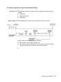
Electrophoresis Circuit
Overview A high-voltage electrical circuit facilitates the electrophoresis of DNA fragments. The
electrical charge is conducted through the circuit by:
♦
DNA and buffer ions in the polymer
♦
Buffer ions in the buffer
♦
Electrons in the electrical wires and electrodes
Diagram The electrophoresis circuit is shown below.
Capillaries containing
polymer
Loading bar
(cathode) (-)
Electrode
(anode) (+)
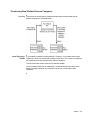
Description During electrophoresis, a high voltage is applied between the loading bar (cathode)
and the electrode located on the lower polymer block (anode). The voltage drives the
movement of negatively charged DNA fragments through the polymer in the capillaries
towards the anode. From the anode, the current flows back in electrical wires through
the power supply to the cathode to complete the circuit.
! WARNING ELECTRICAL SHOCK HAZARD. To reduce the chance of electrical
shock, do not remove covers that require tool access. No user serviceable parts are
inside. Refer servicing to Applied Biosystems qualified service personnel.
2-26 System Overview
Section: Fluorescence Detection Overview
In This Section The following topics are covered in this section:
Topic
See Page
Introduction
2-28
Laser
2-29
Transmission Grating
2-29
CCD Camera
2-29
System Overview 2-27
Introduction
Detection Overview The dye-labeled DNA fragments are separated by electrophoresis within the capillary
array. Once the fragments enter the detection cell, they pass through a laser beam.
The light excites the attached dye labels causing them to fluoresce.
The detection components work together to collect the fluorescence and convert the
information into electronic form. The electronic information is then processed and
displayed by the 3100 Data Collection software.
Detection The main components of the detection system and their function are listed in the
Components following table.
Note
Part
Function
Laser
Excites the attached dye labels as the DNA fragments pass
through the detection cell
Transmission grating
Disperses the light by wavelength and a second set of
lenses focuses the resulting light spectrum onto the CCD
camera
CCD camera
Converts the incident fluorescence into digital information
that is processed by the 3100 Data Collection software
Note
2-28 System Overview
The many lenses and mirrors integral to detection are not covered in this section.
More information on each of the components follows this section.
Laser
Overview When a dye-labeled DNA fragment moves into the path of the laser beam, some
electrons in the dye are excited to higher energy levels as the laser light is absorbed.
Shortly afterwards, the electrons return to their ground states and emit fluorescence
light energy. The light emitted from each dye has a different spectral profile (color).
Laser Type The laser used to excite the dyes is an argon-ion laser.
Emission The primary emission lines are at 488 nm and 514.5 nm.
Wavelengths
Interlock For your safety, an interlock switch shutters the laser and shuts off the electrophoresis
power supply if the doors of the instrument are opened.
For more information on laser safety, refer to the ABI PRISM 3100 Genetic Analyzer
Site Preparation and Safety Guide (P/N 4315835).
! WARNING LASER HAZARD. Exposure to direct or reflected laser light at 40 mW for 0.1
seconds can burn the retina and leave permanent blind spots. Never look directly into the laser
beam or allow a reflection of the beam to enter your eyes.
Transmission Grating
Overview The transmission grating is a grooved disk that spectrally separates the fluorescence
emitted (light) from the dye-labeled DNA fragments. After the light is spectrally
separated, it is focused onto the charge-coupled device (CCD) camera.
CCD Camera
Overview The CCD camera includes a rectangular silicon chip that converts the incident
fluorescence light into digital information.
This digital information (data) will be processed by the 3100 Data Collection software.
A description of the role of the CCD camera in data processing starts on page A-3.
System Overview 2-29
Performing a Run
3
3
Overview
In This Chapter The following topics are covered in this chapter:
Topic
See Page
Section: Introduction
3-3
Summary of Procedures
3-4
Planning Your Runs
3-5
Section: Working with Samples and Plate Assemblies
3-7
Sample Preparation
3-8
Working with Plate Assemblies
3-9
Section: Starting the 3100 System
3-11
Starting the Computer
3-12
Starting the Instrument
3-13
Starting the 3100 Data Collection Software
3-14
Section: Checking the Available Space and Deleting Records
3-15
Checking the Available Hard Drive Space
3-16
Checking the Available Database Space
3-17
Deleting Records from the Database
3-17
Section: Preparing the Instrument
3-19
Instrument Setup
3-20
Preparing Buffer and Filling the Reservoirs
3-22
Calibrating the Instrument
3-24
Placing the Plate onto the Autosampler
3-25
Section: Setting Up the Software
3-27
Setting Software Preferences
3-28
About Plate Records
3-30
Creating a Plate Record for GeneScan Analysis
3-31
Creating a Plate Record for DNA Sequencing Analysis
3-36
Linking and Unlinking a Plate
3-41
Section: Running the Instrument
3-45
About Run Scheduling
3-46
Controlling the Run
3-47
Performing a Run 3-1
Topic (continued)
3-2 Performing a Run
See Page
Run Times
3-48
Section: Monitoring a Run
3-49
Run View Page
3-50
Status View Page
3-51
Array View Page
3-53
Capillary View Page
3-56
Instrument Status Monitor
3-57
Section: Working with Data
3-59
Recovering Data if Autoextraction Fails
3-60
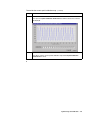
Viewing Raw Data from a Completed Run in the Data Collection Software
3-61
Viewing Analyzed GeneScan Data
3-62
Viewing Analyzed DNA Sequencing Data
3-63
Archiving Data
3-64
Section: Introduction
In This Section The following topics are covered in this section:
Topic
See Page
Summary of Procedures
3-4
Planning Your Runs
3-5
Performing a Run 3-3
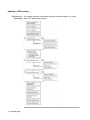
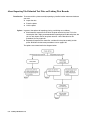
Summary of Procedures
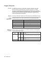
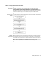
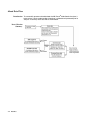
Flowchart of a This flowchart provides an overview of the steps required to perform a run on the
Typical Run ABI PRISM ® 3100 Genetic Analyzer.
3-4 Performing a Run
Planning Your Runs
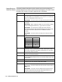
Decisions to Make The main decisions you will need to make when preparing for a run are listed below.
Decision Table
Decision
Comments
Analysis application
Either:
♦ ABI PRISM ® GeneScan® Analysis software for fragment
analysis
♦ ABI PRISM ® DNA Sequencing Analysis software for sequencing
or Rapid DNA Sequencing Analysis
Type of polymer
Either:
♦ ABI PRISM ® 3100 POP-4TM for fragment analysis
♦ ABI PRISM ® 3100 POP-6TM for DNA sequencing or rapid DNA
sequencing
Length of capillary
array
Either:
♦ 36-cm array for fragment analysis or rapid DNA sequencing
♦ 50-cm array for DNA sequencing
Type of plate
Either a:
♦ 96-well plate
♦ 384-well plate
Method of creating
plate records
There are six different ways to create plate records.
Which analysis
module to use
Either:
♦ Select one of the supplied analysis modules
♦ Create your own analysis module in the downstream
application.
Which run module to
use
Either:
♦ Select one of the supplied run modules
♦ Edit one of the supplied run modules to change the conditions
used for a run
How many times to run
your samples
To run your samples only once, use only one run module column
and one analysis module column when creating the plate record.
To run each sample up to five times, use identical run module
columns and identical analysis module columns.
Whether to run the
same sample again
under different run
conditions
Prepare two run module columns when creating the plate record,
filling in the second with a different run module.
Whether to perform a
single run or a batch
run
Either:
♦ A single run that electrophoreses up to 16 samples
♦ A batch run that performs several sequential runs without
needing operator attention
Performing a Run 3-5
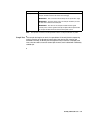
Decision Table
(continued)
Decision
Comments
Whether to save data
to a BioLIMS™
database (optional) or
to ABIF sample files
If you do not enable BioLIMS in the Setting Preferences dialog
box, the sample files are stored in the following directory:
Whether to perform a
spatial calibration
A spatial calibration must be performed after each time you:
D:\AppliedBio\abi\3100\Data Extractor\Extracted Runs
♦ Install or replace a capillary array
♦ Temporarily remove the capillary array from the detection block
Whether to perform a
spectral calibration
A spectral calibration must be performed:
♦ Whenever you use a new dye set on the instrument
♦ Whenever you change the type of polymer used
♦ After the laser or CCD camera has been realigned by a service
engineer
♦ If you begin to see a decrease in spectral separation (pull-up
and/or pull-down peaks)
3-6 Performing a Run
Section: Working with Samples and Plate Assemblies
In This Section The following topics are covered in this section:
Topic
See Page
Sample Preparation
3-8
Working with Plate Assemblies
3-9
Performing a Run 3-7
Sample Preparation
References for For information on required materials, sample preparation, and plate centrifugation,
Sample Preparation refer to the appropriate guide as follows:
For...
Refer to the...
DNA sequencing samples
ABI PRISM Automated DNA Sequencing Chemistry Guide
(P/N 4305080)
Fragment analysis samples
ABI PRISM 3100 Genetic Analyzer Quick Start Guide for
Fragment Analysis (P/N 4315832)
Checking the Plate After centrifuging the plate of samples, ensure each sample is positioned at the
bottom of its tube or well.
To check the plate of samples:
Step
1
Action
Hold the plate up to a light source. Your samples should:
Look like this...
Not look like this...
Not look like this...
The sample is positioned
correctly in the bottom of
the well.
The sample lies on the
side wall because the
plate was not
centrifuged.
An air bubble lies at the
bottom of the well
because the plate was
not:
♦ Centrifuged with
enough force, or
♦ Centrifuged for
enough time
2
3-8 Performing a Run
If any of the samples are not positioned at the bottom of their tube or well,
recentrifuge the plate.
Working with Plate Assemblies
Plate Assembly The plate assembly components are assembled as follows:
Components
Plate retainer
Septa
1
2
3
Sample plate
Plate base
Preparing a Plate To prepare a plate assembly:
Assembly
Step
1
Action
Secure a clean and dry septa strip on the sample plate.
IMPORTANT Never use warped plates.
IMPORTANT Ensure the septa strip lies flat on the plate.
2
Place the sample plate into the plate base.
3
Snap the plate retainer onto the plate and plate base.
Performing a Run 3-9
To prepare a plate assembly: (continued)
Step
4
Action
Ensure the plate retainer holes are aligned with the holes in the septa strip.
IMPORTANT Damage to the array tips will occur if the plate retainer and septa
strip holes do not align correctly.
The plate retainer holes
must align with the holes in
the septa strip.
3-10 Performing a Run
Section: Starting the 3100 System
In This Section The following topics are covered in this section:
Topic
See Page
Starting the Computer
3-12
Starting the Instrument
3-13
Starting the 3100 Data Collection Software
3-14
Performing a Run 3-11
Starting the Computer
Starting the IMPORTANT You must start the computer workstation before starting the ABI PRISM ® 3100
Computer Genetic Analyzer.
Workstation To start the computer workstation:
Step
Action
1
Turn on the monitor.
2
Power on the computer.
The computer boots and then the Begin Logon dialog box appears.
3
Press CTRL + ALT + DELETE and enter the user name and password.
Note
♦ The default user name for the workstation is 3100User. Do not change this user
name.
♦ There is no default password. If you would like to use a password, your system
administrator can create one.
♦ If the computer is connected to a network, you do not need to log on to the
network before starting the instrument.
♦ OrbixWebTM Daemon will launch automatically. If it does not launch, repeat steps
1–3.
3-12 Performing a Run
Starting the Instrument
Starting the To start the 3100 Genetic Analyzer:
Instrument
Step
1
Action
Ensure that the:
♦ Oven door is closed and locked
♦ Instrument doors are closed
Note
2
If the doors are open during power-up, the red failure light will illuminate.
Ensure that the:
♦ Computer is powered on (see “Starting the Computer” on page 3-12)
♦ Microsoft® Windows NT® operating system has loaded
Note The computer must be on and running the Windows NT operating system
because the instrument must copy the firmware from the computer.
3
Turn on the instrument by pressing the on/off button on the front of the instrument.
Status lights
Press the on/off button to start the instrument
Note While the instrument is booting up and performing self-checks, the yellow
status light will blink.
4
Ensure the green status light is on and constant before proceeding.
Note If the green light does not come on, start the ABI PRISM ® 3100 Data
Collection software and look at the event log. If this is not helpful, call a Technical
Support representative. See Appendix B, “Technical Support.”
Performing a Run 3-13
Starting the 3100 Data Collection Software
Before You Begin Before starting the Data Collection software:
Step
Action
1
Ensure the ABI PRISM ® 3100 Genetic Analyzer is powered on and that the green
status light is on solid (not flashing).
2
Ensure OrbixWeb Daemon is running by finding its button on the Windows NT
taskbar.
If OrbixWeb Daemon is not running, go to the Start menu, point to Applied
Biosystems, and select OrbixWeb Daemon.
Note To create a shortcut: (a) Navigate to orbixd.exe in the following directory:
D:\dbtools\iona\orbixweb3.2\bin. (b) Right-click the file. (c) Click Create Shortcut.
This creates a shortcut named Shortcut to orbixd.exe. (d) Drag the shortcut to the
desktop.
IMPORTANT OrbixWeb Daemon must be started before the 3100 Data Collection
software can run.
Starting the Data To start the Data Collection software:
Collection Software
Step
1
Action
From the Start menu, point to Applied Biosystems, and select 3100 Data
Collection.
Note To create a shortcut: (a) Navigate to 3100Collection.bat in the following
directory: D:\AppliedBio\abi\3100\Bin. (b) Right-click the file. (c) Click Create
Shortcut. This creates a shortcut named Shortcut to 3100 Collection Software.
(d) Drag the shortcut to the desktop.
The 3100 Data Collection software opens and the following window is displayed:
3-14 Performing a Run
Section: Checking the Available Space and Deleting Records
In This Section The following topics are covered in this section:
Topic
See Page
Checking the Available Hard Drive Space
3-16
Checking the Available Database Space
3-17
Deleting Records from the Database
3-17
Introduction Before a run or batch of runs, check the available space to ensure there is sufficient
space to store the data you will create. Every week, delete records in the database.
The sections that follow tell you:
♦
How to check the available hard drive space on drive D for the extracted sample
files
♦
How to check the available space in the instrument database on drive E for the
raw data
♦
Where to find the procedures for deleting database records
Performing a Run 3-15
Checking the Available Hard Drive Space
Checking Hard To check the hard drive for space for sample files:
Drive Space
Step
Action
1
Double-click the My Computer icon on the desktop to view the drives.
2
Right-click on a the D drive and select Properties.
The Properties dialog box opens displaying the used and free space.
3
Estimate how much free space you need by using the information provided below.
File Type
Approximate Space
Required Per File (kB)a
Analyzed sample file for DNA sequencing
250
Analyzed sample file for fragment analysis
500
Unanalyzed sample file
100
a. The values provided are estimates only. The actual file size depends on the run
module selected.
4
If there is insufficient space:
a. Archive the sample files to another volume.
b. Delete the original files from the drive.
3-16 Performing a Run
Checking the Available Database Space
Checking Database Note The instrument database automatically expands from 2–9 GB, depending on the
Space amount of data that needs to be stored.
To check the database space:
Step
1
Action
Run the Diskspace utility.
For instructions, see “Checking Database Space: The Diskspace Utility” on
page 7-5.
2
If the used space is more than 8 GB, purge the database of some or all data. See
the procedure references below.
Deleting Records from the Database
Cleanup Database See page 7-8 to run the Cleanup Database utility:
Utility Reference ♦ Once per week, or
♦
When the used space is more than 8 GB, or
♦
Every 400–500 runs
Deleting an Delete individual plate records when you want to free database space without deleting
Individual Plate all of the records (see page 6-39).
Record Reference
Performing a Run 3-17
3-18 Performing a Run
Section: Preparing the Instrument
In This Section The following topics are covered in this section:
Topic
See Page
Instrument Setup
3-20
Preparing Buffer and Filling the Reservoirs
3-22
Calibrating the Instrument
3-24
Placing the Plate onto the Autosampler
3-25
Performing a Run 3-19
Instrument Setup
Using Manual While you are setting up the instrument, you may find manual control useful. For
Control example, you can use manual control commands to move the syringe plungers up and
down, open or close the pin valve, and turn on the oven before starting your run. For a
complete list of the commands, and instructions for using them, see “Controlling the
Instrument Using Manual Control” on page 5-15.
Attaching the To attach the polymer blocks to the instrument:
Polymer Blocks
Step
Action
1
If necessary, clean the polymer blocks and the tubing as instructed on page 8-27.
2
Push the upper polymer block onto the two guide pins on the instrument.
3
Install the lower polymer block. Ensure the block is pushed all the way against the
instrument.
4
Connect the tubing between the two blocks.
a. Insert one ferrule into the upper polymer block and rotate clockwise until finger
tight.
b. Insert the other ferrule into the lower polymer block and rotate clockwise until
finger tight.
IMPORTANT Do not overtighten.
5
Install clean drip trays if they are not already on the instrument.
Preparing and IMPORTANT Wear gloves while performing the following procedure, and any other time you
Installing the handle the capillary array, glass syringes, septa, or buffer reservoirs.
Syringes To prepare and install the syringes:
Step
3-20 Performing a Run
Action
1
Clean and inspect the syringes as instructed on page 8-21.
2
Prime and fill the syringes as instructed on page 8-22.
3
Install the syringes as instructed on page 8-23.
Installing or If necessary, install a capillary array using the Install Capillary Array wizard. For
Replacing the instructions, see “Installing and Removing the Capillary Array” on page 8-15.
Capillary Array
Adding or Changing Determine whether to add or change the polymer on the instrument before proceeding
Polymer with instrument preparation.
If polymer on the instrument is...
Then...
less than 1 week old, and
Ensure there are no air bubbles, and then proceed
with instrument preparation.
sufficient in quantity to complete
your runsa
greater than 1 week old, or
insufficient in quantity to complete
your runs
Note
To remove any air bubbles, see page 8-28.
Fill the syringes and the upper polymer block with
polymer by following the Change Polymer wizard. For
instructions, see page 8-10.
! CAUTION CHEMICAL HAZARD. POP polymer
may cause eye, skin, and respiratory tract irritation.
Please read the MSDS, and follow the handling
instructions. Wear appropriate protective eyewear,
clothing, and gloves. Use for research and
development purposes only.
a. A run uses 50–80 µL of polymer. This is equivalent to 60–100 runs from one 5-mL syringe. A minimum of
1 mL of polymer is required for the instrument to operate.
IMPORTANT Always replace polymer that is older than 1 week.
IMPORTANT Ensure there are no air bubbles in the upper polymer block before proceeding.
To remove any air bubbles, see page 8-28.
Performing a Run 3-21
Preparing Buffer and Filling the Reservoirs
Required Materials The following materials are required to prepare 3100 1X running buffer:
♦
ABI PRISM ® 3100 10X Running Buffer with EDTA (P/N 402824)
♦
Quality deionized water
Making Buffer for a To prepare 50 mL of 1X running buffer:
Single Run
Step
Action
1
Add 5.0 mL of 10X running buffer into a graduated cylinder.
2
Add deionized water to bring the total volume up to 50 mL.
3
Mix well.
Storing the Buffer The 3100 1X running buffer can be stored at 2–8 °C for up to 1 month.
When to Replace the Replace the 1X running buffer in the anode buffer reservoir and the cathode buffer
Buffer reservoir daily, or before each batch of runs.
IMPORTANT Failing to replace buffer may lead to loss of resolution and data quality.
IMPORTANT Replenishing buffer and placing the plate requires that the autosampler be in the
forward position, with the capillary tips removed from the buffer solution. Do not leave the
autosampler in this position for an extended time because the capillaries can dry out.
Filling the Water IMPORTANT Wear gloves while performing the following procedure, and any other time you
and Cathode Buffer handle the capillary array, glass syringes, septa, or buffer reservoirs.
Reservoirs To fill the water and cathode buffer reservoirs:
Step
Action
1
Close the instrument doors.
2
Press the Tray button on the outside of the instrument to bring the autosampler to
the forward position.
Tray button
3
Wait until the autosampler has stopped moving, and then open the instrument
doors.
4
Remove the cathode buffer reservoir and water reservoirs from the instrument.
5
Dispose of remaining fluids and rinse out the reservoirs with deionized water.
Note The waste is very dilute; however, you should follow your company’s waste
disposal practices for appropriate disposal procedures.
6
3-22 Performing a Run
Rinse the cathode reservoir with 1X running buffer, and then fill to the line with 1X
running buffer (about 16 mL).
To fill the water and cathode buffer reservoirs: (continued)
Step
Action
7
Fill the water reservoirs to the line with quality deionized water (about 16 mL).
8
Place a clean septa strip on each reservoir, and dry the outside of the reservoirs
using a lint-free wipe.
! CAUTION Be sure that the septa fit snugly and flush on the tops of the
reservoirs in order to prevent damaging the capillary tips.
Septa is lying flat on the reservoir
Fill line
9
Place the reservoirs into position on the autosampler as shown below.
Water reservoir
(rinse)
4
2
1
Water reservoir
(waste)
Water reservoir
Cathode reservoir
(1X running buffer)
3
Filling the Anode Change the anode buffer:
Buffer Reservoir ♦ Before each run, or at least every 24 hours
♦
Every time you fill the polymer block with new polymer
To fill the anode buffer reservoir to the fill line with 1X running buffer:
Step
Action
1
Remove the anode buffer reservoir by firmly pulling down and twisting slowly.
2
Discard the used buffer appropriately.
3
Clean and rinse the reservoir with deionized water, and then rinse with buffer.
4
Fill the reservoir to the fill line with fresh 1X running buffer (about 9 mL).
Fill line
Performing a Run 3-23
To fill the anode buffer reservoir to the fill line with 1X running buffer: (continued)
Step
5
Action
Put the anode buffer reservoir on the instrument.
Note
6
The meniscus should line up with the fill line.
If the reservoir fills with fluid, repeat this procedure to discard and replace the
running buffer.
Note
The reservoir could fill during bubble clearing.
Calibrating the Instrument
When to Perform a If necessary, perform a spatial calibration.
Spatial Calibration
A spatial calibration must be performed after each time you:
♦
Install a capillary array
♦
Replace a capillary array with a new one
♦
Temporarily remove the capillary array from the detection block
For instructions, see “Spatial Calibration” on page 4-3.
When to Perform a If necessary, perform a spectral calibration.
Spectral Calibration
A spectral calibration must be performed:
♦
Whenever you use a new dye set on the instrument
♦
After the laser has been realigned by a service engineer
♦
After the CCD camera has been realigned by a service engineer
♦
If you begin to see pull-up and/or pull-down peaks consistently
For instructions, see “Spectral Calibration” on page 4-15.
3-24 Performing a Run
Placing the Plate onto the Autosampler
Placing the Plate To place the plate onto the autosampler:
onto the
Step
Action
Autosampler
1
Place the plate assembly on the autosampler as shown below.
Note There is only one orientation for the plate, with the notched end of the plate
base away from you.
IMPORTANT Ensure the plate assembly fits flat in the autosampler. Failure to do
so may allow the capillary tips to lift the plate assembly off of the autosampler.
2
When the plate is correctly positioned, the plate position indicator on the Plate View
page changes from gray to yellow.
Check to ensure this has happened.
Plate placed in position A
No plate in position B
3
Close the instrument doors.
Note Closing the doors returns the autosampler to the home position, placing the
tips of the capillaries in buffer.
Performing a Run 3-25
3-26 Performing a Run
Section: Setting Up the Software
In This Section The following topics are covered in this section:
Topic
See Page
Setting Software Preferences
3-28
About Plate Records
3-30
Creating a Plate Record for GeneScan Analysis
3-31
Creating a Plate Record for DNA Sequencing Analysis
3-36
Linking and Unlinking a Plate
3-41
Performing a Run 3-27
Setting Software Preferences
Introduction The Data Collection software preferences are set during instrument installation;
however, you can view or change these preferences in the Setting Preferences dialog
box.
Viewing the Setting To view the Setting Preferences dialog box:
Preferences
Step
Action
Dialog Box
1
From the View menu, select Preferences or click the Preferences button on the
toolbar.
The dialog box has two pages as described below.
Data Collection Page
The following table describes the preferences that can be set within this page:
Preference
Description
Instrument Name
This field automatically populates with demo_3100.
You can change it to any name (e.g., the instrument’s serial number).
3-28 Performing a Run
Data Analysis Page
The following table describes the preferences that can be set within this page:
Preference
Description
AutoAnalysis On
Select AutoAnalysis On to have the samples automatically analyzed
by the analysis software after the run.
Note Selecting this option will not prevent you from reanalyzing your
sample data.
BioLIMS
Use these settings to have data extracted to a BioLIMS database
instead of to sample files on the hard drive.
Sample File Name
Prefix Format
Specify the format for the sample file names by using the drop-down
lists to reorder the identifiers.
Identifier
Origin
Run ID
Generated by the Data Collection software
Sample Name
Taken from the Plate Editor spreadsheet entry
Well Position
Taken from the sample’s position on the plate
(column letter and row number, e.g., C3)
Plate Name
Taken from the Plate Editor dialog box entry
Instrument ID
Taken from the Data Collection page preferences
entry
Array ID
Taken from the Install Capillary Array wizard
entry
Note In addition to the four identifiers you set with the drop-down
lists, all names are automatically appended with the capillary number
and a file extension. Therefore, in the Data Analysis page example
shown above, the sample name will be:
Sample Name_Well Position_Capillary Number.fsa (or .abl for
sequencing)
Performing a Run 3-29
About Plate Records
Introduction A plate record is similar to a sample sheet or an injection list that you may have used
with other ABI PRISM ® instruments.
Plate records are data tables in the instrument database that store information about
the plates and the samples they contain. Specifically, a plate record contains the
following information:
♦
Plate name, type, and owner
♦
Position of the sample on the plate (well number)
♦
Sample name
♦
Dye color of size standard, if present (GeneScan analysis only)
♦
Mobility file (DNA sequencing analysis only)
♦
Comments about the plate and about individual samples
♦
Dye set information
♦
BioLIMS project (this entry is mandatory, even when BioLIMS is not used)
♦
The name of the run module (run modules specify information about how samples
are run)
♦
The name of the analysis module (analysis modules specify how raw data is
autoanalyzed at the end of the run)
When to Create a A plate record must be created for each plate of samples for the following types of
Plate Record runs:
♦
Fragment analysis
♦
DNA sequencing
♦
Spectral calibrations
Note For fragment analysis and sequencing runs, there is no need to re-create a plate record
for a plate that has failed. Simply edit the plate record to add a run module and an analysis
module column to the rows that need to be re-run. This will move the existing plate record from
the Processed window to the Pending window.
Create plate records in advance of placing the plates on the instrument.
A plate record cannot be created while a run is in progress.
About the Procedure The next two sections cover the most common method for creating a plate record.
There is a separate procedure for each analysis application.
Note There are several other methods for creating a plate record. See Chapter 6, “Working
with Plate Records.”
Plate Records for For information on creating plate records for spectral calibration runs, see “Creating a
Spectral Runs Plate Record” on page 4-21.
3-30 Performing a Run
Creating a Plate Record for GeneScan Analysis
Entering Plate Note You cannot create a plate record while a run is in progress.
Record Information
To enter plate record information:
Step
1
Action
Click the Plate View tab on the 3100 Data Collection software window to go to the
Plate View page.
Plate View tab
2
On the Plate View page, click New. Or, click the Plate Editor button on the toolbar.
The Plate Editor dialog box appears.
3
Use the Plate Editor dialog box to name your plate and to specify the application
and plate type. Entering comments is optional.
IMPORTANT When naming the plate, you can use letters, numbers, and the
following punctuation only: -_(){}#.+. Do not use spaces.
4
When done, click Finish.
The Plate Editor spreadsheet opens.
Performing a Run 3-31
Entering Sample To enter sample information and save the plate record:
Information
Step
1
Action
In the Plate Editor spreadsheet, type the names of all the samples in the Sample
Name column.
Note In the default naming convention, the sample name you type is incorporated
into the sample file name. For example:
MySample_A01_01.fsa
Capillary position
Well position
Sample name you type
The sample file naming convention used can be changed in the Preferences dialog
box. See page 3-28 for details.
IMPORTANT When naming the samples, you can use letters, numbers, and the
following punctuation only: -_(){}#.+. Do not use spaces.
IMPORTANT Be sure that sample file names are not longer than 55 characters.
An underscore separates each preference selected, so be sure to count the
underscore in the number of characters. There is no automatic error checking for
sample names that exceed this limit. Sample files with long names cannot be
opened by the analysis software.
2
Optional
For each sample, enter Color Info and Color Comment text.
3
Enter a BioLIMS project.
IMPORTANT A BioLIMS project is required for every sample, even if a BioLIMS
database is not used.
a. Click in the BioLIMS Project cell for Well A1.
b. Select a project name from the drop-down list.
IMPORTANT You must enter a BioLIMS
Note
To set up a BioLIMS project, see page 5-48.
c. To assign the same project name to each sample in the plate record:
– Click the column header to select the whole column.
– Press CTRL+D.
Note Press CTRL+D whenever a field is the same for all samples in the plate
record.
3-32 Performing a Run
\
To enter sample information and save the plate record: (continued)
Step
4
Action
For each sample, select the appropriate Dye Set from the drop-down list.
For GeneScan analysis, select Dye Set D.
IMPORTANT Be sure to select the correct dye set for your run(s). Data collected
with the incorrect dye set selected cannot be saved and the runs will have to be
repeated because multicomponenting is applied during collection.
5
For each sample, select the appropriate Run Module from the drop-down list.
The following table shows the run module to select based on your run type:
Analysis Type
Run Module
GeneScan
GeneScan36_POP4DefaultModule
Note
If you need to view or edit a run module file, see page 5-20.
Note If you select different modules for different samples, the samples will be
automatically grouped so that all samples with the same run module are run at the
same time. Runs are scheduled alphanumerically by run module name, not by the
order indicated in the plate record, nor by sample name.
Performing a Run 3-33
To enter sample information and save the plate record: (continued)
Step
6
Action
For each sample, select the appropriate Analysis Module from the drop-down list.
IMPORTANT The AutoAnalysis On preference must be selected if analysis is to
take place automatically after the run (see page 3-29).
The following table shows which analysis module to select based on the number of
fragments in your size standard:
If using size standard...
Select this analysis module...
GS400HD
GS400HDAnalysis.gsp
GS350
GS350Analysis.gsp
GS500
GS500Analysis.gsp
GS500 (see footnote)
GS400CubicAnalysis.gspa
GS400Ord2Analysis.gspa
a. These modules are for advanced users with specific sizing needs. See the ABI PRISM
GeneScan Analysis Software v. 3.5 NT User’s Manual.
Note You can examine the settings for each of these files using GeneScan
Analysis Software. The meanings of the settings are described in the ABI PRISM
GeneScan Analysis Software v. 3.6 NT User’s Manual.
Note
7
For more information on module files, see Chapter 5, “Software.”
If you want to run the same sample again, select a second run module and a
second analysis module. You can run a sample in a linked plate up to five times.
Samples will be automatically grouped so that all samples with the same run
module are run sequentially.
3-34 Performing a Run
To enter sample information and save the plate record: (continued)
Step
8
Action
Make sure the plate record is correct, and then click OK.
Note It may take a while for the new plate record to be saved to the database and
added to the Pending Plate Records table as shown below.
Performing a Run 3-35
Creating a Plate Record for DNA Sequencing Analysis
Entering Plate Note You cannot create a plate record while a run is in progress.
Record Information
To enter plate record information:
Step
1
Action
Click the Plate View tab on the 3100 Data Collection software window to go to the
Plate View page.
Plate View tab
2
In the Plate View page, click New. Or, double-click the Plate Editor button on the
toolbar.
The Plate Editor dialog box appears.
3
Use the Plate Editor dialog box to name your plate and to specify the application
and plate type. Entering comments is optional.
IMPORTANT When naming the plate, you can use letters, numbers, and the
following punctuation only: -_(){}#.+. Do not use spaces.
4
When done, click Finish.
The Plate Editor spreadsheet opens.
3-36 Performing a Run
Entering Sample To enter sample information and save the plate record:
Information
Step
1
Action
In the Plate Editor spreadsheet, type the names of all the samples in the Sample
Name column.
Note In the default naming convention, the sample name you type is incorporated
into the sample file name. For example:
MySample_A01_01.ab1
Capillary position
Well position
Sample name you type
\
The sample file naming convention used can be changed in the Preferences dialog
box. See page 3-28 for details.
IMPORTANT When naming the samples, you can use letters, numbers, and the
following punctuation only: -_(){}#.+. Do not use spaces.
IMPORTANT Be sure that sample file names are not longer than 55 characters.
An underscore separates each preference selected, so be sure to count the
underscore in the number of characters. There is no automatic error checking for
sample names that exceed this limit. Sample files with long names cannot be
opened by the analysis software.
2
For each sample, select the appropriate Dye Set from the drop-down list.
For DNA Sequencing analysis, select Dye Set E.
IMPORTANT Be sure to select the correct dye set for your run(s). Data collected
with the incorrect dye set selected cannot be saved and the runs will have to be
repeated because multicomponenting is applied during collection.
Performing a Run 3-37
To enter sample information and save the plate record: (continued)
Step
3
Action
For each sample, select the appropriate Mobility File from the drop-down list.
Note You may need to resize the column to see the whole file name. To do this,
place the cursor between the column headers (it will become a double-headed
arrow) and drag right.
The following table shows which mobility file to select based on your sequencing
chemistry:
4
DNA Sequencing Chemistry
Mobility File
ABI PRISM ® BigDyeTM Primer chemistry;
using the -21m13 primer
DP3100POP6{BD-21M13}v1.mob
BigDye Primer chemistry; using the
reverse primer
DP3100POP6{BD-M13Rev}v1.mob
ABI PRISM ® BigDyeTM Terminator
chemistry
DT3100POP6{BD}v2.mob
ABI PRISMTM dRhodamine Terminator
chemistry
DT3100POP6{dRhod}v1.mob
Enter a BioLIMS project.
IMPORTANT A BioLIMS project is required for every sample, even if a BioLIMS
database is not used.
a. Click in the BioLIMS Project cell for Well A1.
b. Select a project name from the drop-down list.
IMPORTANT You must enter a BioLIMS project.
Note
To set up a BioLIMS project, see page 5-48.
c. To assign the same project name to each sample in the plate record:
– Click the column header to select the whole column.
– Press CTRL+D.
– The Project Name for every sample in the plate record is now the same.
Note Press CTRL+D whenever a field is the same for all samples in the plate
record.
3-38 Performing a Run
To enter sample information and save the plate record: (continued)
Step
5
Action
For each sample, select the appropriate Run Module from the drop-down list.
Note
If you need to view or edit a run module file, see page 5-20.
The following table shows the run module to select based on your run type.
Analysis Type
Run Module
Standard DNA sequencing
StdSeq50_POP6DefaultModule
Rapid DNA sequencing
RapidSeq36_POP6DefaultModule
Note If you select different modules for different samples, the samples will be
automatically grouped so that all samples with the same run module are run at the
same time. Runs are scheduled alphanumerically by run module name, not by the
order indicated in the plate record, nor by sample name. To see the scheduled order
of the runs, select the Run View tab.
6
For each sample, select the appropriate Analysis Module from the drop-down list.
IMPORTANT The AutoAnalysis preference must be selected if analysis is to take
place automatically after the run (see page 3-29).
The following table shows the analysis module to select based on your run type:
Run Type
Analysis Module
Standard DNA sequencing
BC-3100_SeqOffFtOff.saz
Rapid DNA sequencing
BC-3100RR_SeqOffFtOff.saz
Note You can examine the settings for each of these files using DNA Sequencing
Analysis software. The meanings of the settings are described in the ABI PRISM
DNA Sequencing Analysis Software v. 3.6 NT User’s Manual.
7
If you want to run the same sample again, select a second run module and a
second analysis module. You can run a sample in a linked plate up to five times.
Samples will be automatically grouped so that all samples with the same run
module are run sequentially.
Performing a Run 3-39
To enter sample information and save the plate record: (continued)
Step
8
Action
Make sure the plate record is correct, and then click OK.
Note It may take a while for the new plate record to be saved to the database and
added to the Pending Plate Records table as shown below.
3-40 Performing a Run
Linking and Unlinking a Plate
Introduction The procedure below describes how to link a plate on the autosampler to the plate
record you have created. This must be done before a plate can be run.
IMPORTANT A plate can be linked even if there are no run modules selected for its samples.
In this case, there is no error message and runs for samples in the plate will not be scheduled.
Linking a Plate to a To link a plate to a plate record:
Plate Record
Step
1
Action
Click the Plate View tab on the 3100 Data Collection software window to go to the
Plate View page.
Plate View tab
2
On the Plate View page:
a. In the Pending Plate Records table, click the plate record for the plate you are
linking.
b. Click the plate position indicator that corresponds to the plate you are linking.
Click the plate record
Click anywhere on the plate
position indicator
Performing a Run 3-41
To link a plate to a plate record: (continued)
Step
3
Action
Verify that the plate has been linked.
Once the plate has been linked, the:
♦ Run Instrument button on the toolbar is enabled, meaning that the instrument is
ready to run.
♦ Plate position indicator for the linked plate becomes green.
♦ Plate record moves from the Pending Plate Records table to the Linked Plate
Records table.
Run Instrument
button is enabled
Plate position
indicator is green
Plate record is in the Linked Plate Records table
4
3-42 Performing a Run
Repeat steps 1–3 to link a second plate, if applicable.
To link a plate to a plate record: (continued)
Step
5
Action
Click the Run View tab to view the run schedule.
For more information about the Run View page, see page 3-50.
Note Although individual runs can be deleted, the order in which the runs are
scheduled cannot be altered. For more information on run scheduling, see
page 3-46.
Unlinking a Plate To unlink a plate record:
Record
Step
Action
1
In the Linked Plate Records table of the Plate View page, select the plate record that
you want to unlink.
2
Click Unlink.
If the plate record is...
Then the plate record will...
completed
Go to the Processed Plate Records.
not completed
Return to the Pending Plate Record table, and the
plate position indicator will return to yellow.
Performing a Run 3-43
3-44 Performing a Run
Section: Running the Instrument
In This Section The following topics are covered in this section:
Topic
See Page
About Run Scheduling
3-46
Controlling the Run
3-47
Run Times
3-48
Performing a Run 3-45
About Run Scheduling
Introduction To view the run schedule, click the Run View tab. The order in which the runs are
scheduled cannot be altered. Run scheduling depends on the factors listed below.
Plate Run Order If two plates are being run, the order in which they are run is based on the following
factors, in the order listed:
♦
If one plate is a spectral calibration run, it will be run first.
♦
For two plates of either fragment analysis or DNA sequencing, the plates will be
run in the order in which the plates were linked.
Sample Run Order The order in which the samples are run is based on the following factors, in the order
listed:
♦
First, samples will be sorted alphabetically by run module name.
–
Samples with module names beginning with capital letters come before those
that begin with lower-case letters (e.g., Z before a).
–
If samples have the same run module name, the samples on the plate that
was linked first will be run first.
♦
Secondly, samples within a plate will be run in the order of their well designation
(i.e., A1, B1, C1, etc.).
♦
Lastly, samples with more than one run module specified will be run in the order
that the run modules appear.
Note
3-46 Performing a Run
The analysis module of a sample plays no part in the order in which it will be run.
Controlling the Run
Controlling the Run You can use the Instrument menu to start, skip, pause, or stop a run.
Using the
Instrument Menu
Controlling the Run You can also use the toolbar at the top of the 3100 Data Collection software window to
Using the Toolbar control the run.
To...
Click...
Comment
Start the run
Run Instrument
♦ This begins all scheduled runs.
♦ The run starts only when set
temperature is reached.
Pause the run
Pause
♦ Complete the current run,
and
a. Stop
♦ Stop the other scheduled
runs
♦ Stop the current run, and
b. After run in the Question dialog box
a. Stop
♦ Stop the other scheduled
runs
b. Now in the Question dialog box
♦ Stop the current run, and
♦ Continue the other
scheduled runs
Pausing for long periods may affect data
quality.
Skip to Next Run
When you click Now, the run files extract
automatically. The files will be automatically
analyzed if the AutoAnalysis preference is
enabled.
To recover data from a stopped run, see
“Recovering Data if Autoextraction Fails” on
page 3-60.
To recover data from a stopped run, see
“Recovering Data if Autoextraction Fails” on
page 3-60.
Performing a Run 3-47
Run Times
DNA Sequencing The following table lists the approximate run times of common DNA sequencing
Run Times analysis runs:
Type of Analysis
Run Module
Run Time
Standard DNA sequencing
StdSeq50_POP6DefaultModule
2 hr 30 min
Rapid DNA sequencing
RapidSeq36_POP6DefaultModule
1 hr
GeneScan Run The following table lists the approximate run times of common GeneScan analysis
Times runs:
3-48 Performing a Run
Type of Analysis
Run Module
Run Time
GeneScan
GeneScan36_POP4DefaultModule
45 min
Section: Monitoring a Run
In This Section The following topics are covered in this section:
Topic
See Page
Run View Page
3-50
Status View Page
3-51
Array View Page
3-53
Capillary View Page
3-56
Instrument Status Monitor
3-57
Introduction This section describes the functions and features of:
♦
The 3100 Data Collection software pages that are used to monitor a run, and
♦
The Instrument Status Monitor, which provides a summary of the current run
conditions.
Performing a Run 3-49
Run View Page
Function Click the Run View tab to monitor the status of the scheduled runs.
Features This is an example of the Run View page.
Capillary
use
indicator
Scheduled
runs in order
Plate
images
Reservoir
positions
Delete
button
Run Schedule Each row in the table provides information about a scheduled run. A run can be
selected by single-clicking on a row.
Note Although individual runs can be deleted, the order in which the runs are scheduled
cannot be altered. For more information on run scheduling, see page 3-46.
Capillary Use This grid displays the capillaries in use during a run and the name of the sample that
Indicator will be injected into a specific capillary.
Each cell in the grid represents a specific capillary. Once a run has started, the cells
representing capillaries in use will turn blue. Placing the cursor over an individual cell
will display the name of the sample to be injected in that capillary.
Plate Image The plate images provide a visual representation of the physical sample layout for a
Indicators selected run.
Delete Button The Delete button removes a run from the list of scheduled runs. First select the run in
the Run Schedule window on the left, and then click the Delete button.
Note The Delete button does not delete the samples from the plate record. The samples can
be run later, if desired.
3-50 Performing a Run
Status View Page
Function Click the Status View tab to monitor the status of the instrument during a run.
Features This is an example of the Status View page.
Instrument
Condition
group box
Events
box
Errors
box
Status bar
Actual value
Set value (defined in the selected run module)
Instrument The color of the box provides a quick way to check the status of the item to the right.
Condition Group See the table below for a definition of each color.
Box
For...
A green box
indicates...
A red box
indicates...
A yellow box
indicates...
Laser
Laser is off
Laser is on
Laser is idle
EP
Electrophoresis is off
Electrophoresis is on
—
Oven
Oven is off
Oven is on
—
Front Doors
Doors are closed
Doors are open
—
Oven Door
Door is closed
Door is open
—
Autosampler
Autosampler is homed
Autosampler is forward
—
Events Box The Events box lists the:
♦
Instrument’s recent actions
♦
Status of each capillary as passed or failed at the end of a spectral calibration
♦
Calibration data at the end of a spatial calibration
Some of the events listed in the Events box provide information for service engineers.
Performing a Run 3-51
Errors Box The Errors box lists errors that have occurred during the current run.
Some of the error messages provide information for service engineers. A “fatal” error
usually requires that you restart the Data Collection software.
Status Bar The Status bar indicates the instrument’s current state or operation.
3-52 Performing a Run
Array View Page
Function Click the Array View tab during or after a run to examine the quality of your data, which
is displayed as individual electropherograms and as color data for the entire capillary
array.
IMPORTANT Always exit from the Array View and the Capillary View windows. During a run,
do not leave these pages open for extended periods. This may cause unrecoverable screen
update problems. Leave the Status View window open.
Features This is an example of the Array View page.
Capillary/color data
display
Raw multicomponented
electropherogram display for
selected capillary
Use this scroll box
to view data
block-by-block.
Selected capillary to be
displayed in the center plot
Fluorescence emission spectrum
for the selected capillary
Total intensity of collected
signal for each capillary
Performing a Run 3-53
Capillary/Color Each cell in the capillary/color data display represents one capillary. The status of that
Data Display capillary is indicated by the color of the cell as described in the following table.
Cell Color
Status of the Capillary
Comment
Green
Operational
—
Yellow
Questionable
This capillary did not pass the spectral calibration
and has been assigned the spectral profile of its
nearest passing neighbor.
There may be a problem with data collected from
this capillary.
Red
Nonoperational
All capillaries will have a red cell until a spatial
calibration is performed.
Capillary Display The capillary window displays the signal intensity by capillary number.
Fluorescence The fluorescence emission spectrum displays the real-time fluorescence emission
Emission Spectrum spectrum of the dye-labeled fragments from the capillary selected. The spectrum is
plotted against the CCD bin number instead of wavelength.
Note This window is updated each time you select a different capillary in the Capillary Display
window during data collection.
Electropherogram An electropherogram is a graph of relative dye concentration against time, plotted for
Display each dye. The data displayed has been multicomponented. The relative dye
concentration is determined by applying chemometric algorithms to the collected
fluorescence data.
There are two plots for each dye. The plots represent the upper and lower confidence
limits associated with the measured fluorescence intensity.
3-54 Performing a Run
Total Intensity The total intensity graph is a graph of the total intensity detected for each capillary.
Graph
Note This window works only during data collection. This window is updated each time you
select a different capillary in the Capillary Display window during data collection.
Performing a Run 3-55
Capillary View Page
Function Click the Capillary View tab to examine the quality of electropherogram data for
several capillaries at once.
IMPORTANT Always exit from the Array View and the Capillary View windows. During a run,
do not leave these pages open for extended periods. This may cause unrecoverable screen
update problems. Leave the Status View window open.
Features This is an example of the Capillary View page for a GeneScan run.
Select check boxes of capillaries to be displayed
Electropherogram
displays
Check Boxes Select the check boxes of the capillaries for which you want electropherograms
displayed.
Note Only four capillary electropherograms will fit on the screen at one time. If you select
more than four, a scroll bar appears so that you can access the others.
Electropherogram An electropherogram is a graph of relative dye concentration against time, plotted for
Displays each dye. The data displayed is multicomponented. The relative dye concentration is
determined by applying chemometric algorithms to the collected fluorescence data.
There are two plots for each dye. The plots represent the upper and lower confidence
limits associated with the measured fluorescence intensity.
Display Order
The capillaries are displayed in the order in which the boxes are checked. For
example, to display capillary 1 under capillary 15: (a) Clear all check boxes. (b) Select
check box 15. (c) Select check box 1.
3-56 Performing a Run
Instrument Status Monitor
Function The Instrument Status Monitor displays the current run conditions.
Viewing the To view the Instrument Status Monitor:
Instrument Status
Step
Action
Monitor
1
From the View menu, select Instrument Status Monitor or double-click the
Instrument Status Monitor button on the toolbar.
Note
The Instrument Status Monitor can remain open while viewing other pages.
Performing a Run 3-57
3-58 Performing a Run
Section: Working with Data
In This Section The following topics are covered in this section:
Topic
See Page
Recovering Data if Autoextraction Fails
3-60
Viewing Raw Data from a Completed Run in the Data Collection Software
3-61
Viewing Analyzed GeneScan Data
3-62
Viewing Analyzed DNA Sequencing Data
3-63
Archiving Data
3-64
Performing a Run 3-59
Recovering Data if Autoextraction Fails
Introduction Runs that are stopped before completion display the status Completed in the run table
on the Run View page.
The auto extractor should automatically extract data from stopped runs. If
autoextraction fails, use the Extract data into sample files command as described
below.
Recovering Data To recover data from a stopped run:
from a Stopped Run
Step
Action
1
From the Instrument menu, point to Data Acquisition and select Extract data into
sample files.
2
Look for the message “Sample Files Successfully Extracted” on the Status bar.
Note The extracted data is unanalyzed. Use the analysis software to analyze the
sample files.
3-60 Performing a Run
Viewing Raw Data from a Completed Run in the Data Collection Software
Introduction Raw data is data that has been multicomponented (corrected for spectral overlap) but
mobility correction has not been applied. There are two formats for viewing the raw
data within the 3100 Data Collection software:
♦
In the Array View page (in much the same way that you might view the gel file
output from an ABI PRISM ® slab gel instrument)
♦
In the Capillary View page, capillary-by-capillary
Note Only current run data can be viewed during a run; you cannot view data from previous
runs while the instrument is running.
IMPORTANT Always exit from the Array View and the Capillary View windows. During a run,
do not leave these pages open for extended periods. This may cause unrecoverable screen
update problems. Leave the Status View window open.
Viewing Raw Data To view raw data from a completed run:
Step
Action
1
In the 3100 Data Collection software, click the Array View tab to display the Array
View page.
2
From the Instrument menu, point to Data Acquisition, and choose Display Run Data.
This opens the Select the run to display dialog box.
3
4
From the drop-down list, select the run that you want to display and click OK.
Note
You can view any completed run that remains in the instrument database.
Note
It may take a few moments to retrieve the data.
Use the scroll features on the Array View page to view the data.
Note
For information on the Array View page, see page 3-53.
IMPORTANT Always exit from the Array View and the Capillary View windows.
During a run, do not leave these pages open for extended periods. This may cause
unrecoverable screen update problems. Leave the Status View window open.
5
Alternatively, to view electropherogram data from several capillaries at once, click
the Capillary View tab to display the Capillary View page.
Note
For information on the Capillary View page, see page 3-56.
IMPORTANT Always exit from the Array View and the Capillary View windows.
During a run, do not leave these pages open for extended periods. This may cause
unrecoverable screen update problems. Leave the Status View window open.
Performing a Run 3-61
Viewing Analyzed GeneScan Data
Introduction After a run has been extracted to sample files, you can use the GeneScan Analysis
software to view the electropherogram data, both raw and analyzed.
Refer to the ABI PRISM GeneScan Analysis Software v. 3.5 NT User’s Manual
(P/N 4308923) for details on viewing and analyzing GeneScan data.
Locating Sample When a run is finished, the analyzed sample files are extracted into a run folder, along
Files with a run log, in the directory:
D:\AppliedBio\abi\3100\DataExtractor\ExtractedRuns
An example of the run folder and its contents is shown below.
Run Folder Default The default name of the run folder is:
Name Run_<Instrument name>_<date>_<runID>
An example of a run folder name is shown below.
Run number for the day
Year-month-day
Instrument name
3-62 Performing a Run
Viewing Analyzed DNA Sequencing Data
Introduction After a run has been extracted to sample files, you can use the DNA Sequencing
Analysis software to view the electropherogram data, both raw and analyzed.
Refer to the ABI PRISM DNA Sequencing Analysis Software v. 3.6 NT User’s Manual
(P/N 4308924) for details on viewing and analyzing GeneScan data.
Locating Sample When a run is finished, the analyzed sample files are extracted into a run folder, along
Files with a run log, in the following directory:
D:\AppliedBio\abi\3100\DataExtractor\ExtractedRuns
An example of the run folder and its contents is shown below.
Run Folder Default The default name of the run folder is:
Name Run_<Instrument name>_<date>_<runID>
An example of a run folder name is shown below.
Run number for the day
Year-month-day
Instrument name
Performing a Run 3-63
Archiving Data
Introduction There are many options for archiving your data. You could, for example, copy the data
to another networked computer and from there use any archiving system, such as an
external SCSI storage device.
We do not recommend that you add a SCSI storage device to the computer
workstation. However, if you need to temporarily install one, follow the procedure
below.
IMPORTANT Do not install a SCSI device on the computer workstation before the
3100 Genetic Analyzer has been installed with the 3100 Software. Installing a SCSI device first
will alter the drive letter assignments so that the instrument and software cannot be properly
installed.
Installing a SCSI To install a SCSI storage device:
Storage Device
Step
3-64 Performing a Run
Action
1
Shut down the computer workstation.
2
Plug the device into the external SCSI port.
3
Turn the computer workstation back on.
4
Ensure the drive letter assignments have not changed. See page 2-14.
Spatial and Spectral
Calibrations
4
4
Overview
In This Chapter The following topics are covered in this chapter:
Topic
See Page
Section: Spatial Calibration
4-3
About Spatial Calibrations
4-4
About Spatial Calibration Data
4-5
Performing a Spatial Calibration
4-6
Displaying a Spatial Calibration Profile
4-10
Evaluating a Spatial Calibration Profile
4-11
Overriding the Current Spatial Calibration Map
4-12
Section: Spectral Calibration
4-15
About Spectral Calibrations
4-16
Performing a Spectral Calibration Using Default Processing Parameters
4-18
Displaying a Spectral Calibration Profile
4-25
Overriding a Spectral Calibration Profile
4-28
Section: Advanced Features of Spectral Calibration
4-33
Fine-Tuning a MatrixStandard Calibration
4-34
Spectral Calibration Matrices
4-36
Spectral Calibration Log Files
4-37
Spectral Calibration Parameter Files
4-38
Spectral Calibration Parameters
4-40
dataType Parameter
4-41
minQ Parameter
4-42
conditionBounds Parameter
4-44
numDyes and writeDummyDyes Parameters
4-46
numSpectralBins Parameter
4-46
Parameters Specific to sequenceStandard dataType
4-47
startptOffset Parameter
4-48
maxScansAnalyzed Parameter
4-49
startptRange Parameter
4-49
minRankQ Parameter
4-50
Spatial and Spectral Calibrations 4-1
4-2 Spatial and Spectral Calibrations
Section: Spatial Calibration
In This Section The following topics describe how to perform a spatial calibration:
Topic
See Page
About Spatial Calibrations
4-4
About Spatial Calibration Data
4-5
Performing a Spatial Calibration
4-6
Displaying a Spatial Calibration Profile
4-10
Evaluating a Spatial Calibration Profile
4-11
Overriding the Current Spatial Calibration Map
4-12
Spatial and Spectral Calibrations 4-3
About Spatial Calibrations
When to Calibrate A spatial calibration must be performed after each time you:
♦
Install or replace a capillary array
♦
Temporarily remove the capillary array from the detection block
What a Spatial A spatial calibration provides information about the position of the fluorescence from
Calibration Tells each capillary on the CCD. It does not provide information about the performance of
You the capillaries.
4-4 Spatial and Spectral Calibrations
About Spatial Calibration Data
Spatial Maps The spatial map is a simple numerical table that defines the number of pixels at the
center of the fluorescence from each capillary in the spatial dimension of the CCD.
For information on the organization of the CCD and frame data, refer to Appendix A,
“Data Flow.”
Only one spatial map at a time is stored in the database on drive E. The term “current”
spatial map refers to the spatial map that is currently stored in the instrument
database. You can replace (override) the “current” spatial map stored in the instrument
database with a spatial map stored in a spatial calibration file. For the procedure, see
page 4-12.
The maps are stored as text files in the SpatialCalLogs folder in the following
directory:
D:\AppliedBio\abi\3100\DataCollection\SpatialCalLogs
Spatial maps are also saved to the 3100 Calibration file and to the firmware.
Spatial Calibration Spatial calibration files are stored on drive D.
Files
Each spatial calibration file contains one spatial map from either the current or
previous calibrations.
Spatial calibration files have the following file name format:
SpatialCal-instrumentname-Rundate-time.scl
Spatial Calibration A spatial calibration log file is created during a spatial calibration. It contains a
Log Files summary of the data collected during the spatial calibration run, including the pixel
positions assigned to each capillary.
The log file is a text file that can be opened and viewed in the Notepad accessory. It
can be useful for troubleshooting spatial calibration problems.
The log file is stored in the same directory as the spatial calibration files with the
following file name format:
SpatialCal-instrumentname-Rundate-time.log
Spatial and Spectral Calibrations 4-5
Performing a Spatial Calibration
Performing a Spatial To perform a spatial calibration:
Calibration
Step
1
Action
From the Tools menu, select Perform Spatial Calibration.
The following dialog box appears:
2
Select the Fill capillaries check box if the:
♦ Capillaries have no polymer (i.e., a new capillary array), or
♦ Polymer in the capillaries has been used in a run
Note
3
You need not fill the capillaries each time you perform a spatial calibration.
Click Start. The calibration takes approximately:
♦ 2 min without filling the capillaries
♦ 6 min with filling the capillaries
4-6 Spatial and Spectral Calibrations
To perform a spatial calibration: (continued)
Step
4
Action
If the calibration...
Then...
succeeded
the following dialog box appears:
a. Click Details to view the Spatial Calibration Profile window.
b. Continue on to “Viewing Successful Results and Saving
the Data” below.
failed
an error message box appears, providing some information
about the reason for the failure.
a. Click Details to view the Spatial Calibration Profile window.
b. Do one of the following:
– Click Cancel, and then click Start to repeat the
calibration.
– Take corrective action as outlined on page 4-9.
Spatial and Spectral Calibrations 4-7
Viewing Successful To view the spatial calibration results and save the data:
Results and Saving
Step
Action
the Data
1
Evaluate the spatial calibration profile.
Note For information about the profile, see “Evaluating a Spatial Calibration
Profile” on page 4-11.
When you are finished, click OK to close the Spatial Calibration Profile box.
2
If the spatial calibration
profile is...
Then...
satisfactory
Continue on to step 3.
unsatisfactory
a. Click Cancel to close the Details box, and then
click Start to repeat the calibration, or
b. Reposition one or more of the red crosses. To
move a cross, change the value in the Capillary
Position box, and then click outside of that box.
c. Override the data with data from a previous run
(see page 4-28.)
If the calibration continues to provide unsatisfactory
results, see “If the Calibration Fails” on page 4-9.
3
Click OK to close the Perform Spatial Calibration window.
The Question dialog box opens.
4-8 Spatial and Spectral Calibrations
To view the spatial calibration results and save the data: (continued)
Step
Action
4
To...
Then...
save this calibration data to the
3100 Data Collection Software
database
Click Yes.
delete this data and use data from a
previous run
a. Click No.
b. Proceed to “Overriding the Current
Spatial Calibration Map” on page 4-12.
If the Calibration If the calibration failed, or if you do not like the appearance of the passed calibration
Fails profile, try one or more of the following corrective actions.
♦
Repeat the calibration.
♦
Fill the capillaries with polymer, and then repeat the calibration.
♦
Clean the detection cell, and then repeat the calibration (see page 8-14).
♦
Reposition the array window in the detection cell, and then repeat the calibration.
Spatial and Spectral Calibrations 4-9
Displaying a Spatial Calibration Profile
Introduction By performing the procedure below, you can display the spatial calibration profile for
the current capillary array or the profile that was used for a previous run.
Note With this procedure, you can view spatial calibration data, but you cannot change which
data is set as the current map.
Displaying a Spatial To display a spatial calibration profile:
Calibration Profile
Step
1
Action
From the Tools menu, select Display Spatial Calibration.
This opens the Question dialog box.
2
If you want to display
the profile for...
Then...
the current array
Click Current Array.
This opens the Spatial Calibration Profile box for the
current calibration data.
Note The title bar is now displayed as Current
Spatial Calibrations.
a previous run
a. Click Previous run.
b. Select the desired run in the Select the source to
display dialog box.
c. Click OK.
Note For information about the profile, see “Evaluating a Spatial Calibration
Profile” on page 4-11.
4-10 Spatial and Spectral Calibrations
Evaluating a Spatial Calibration Profile
Evaluation Criteria While viewing the calibration profile in the Details dialog box, use the following criteria
to evaluate the data:
Peak Attribute
Criteria
Height
Similar heights for all peaks.
Red crosses
One red cross marking the top of every peak. No misplaced crosses.
To move a cross: (a) Change the value in a Capillary Position box.
(b) Click outside of that box. (c) Click OK to accept the new value.
Shape
♦ Single sharp peak for each capillary.
♦ Small shoulders are acceptable.
Spacing
Position values are 13–16 higher than the previous one for every capillary.
Theoretical spacing between capillaries is 15.
Example of Passing
Profile
Example of Failed
Profile
Spatial and Spectral Calibrations 4-11
Overriding the Current Spatial Calibration Map
Introduction Once the spatial calibration run has completed and you have accepted it, the new
spatial calibration map is stored in the instrument database and sent to the
instrument. This new map will be used to process sample run data.
If the current run did not provide good data, you can override the new data with:
♦
Data collected during a previous run on the same capillary array if the detection
cell has not been moved
♦
A spatial calibration map used to process any previous sample run still stored in
the database
When overriding the data with data from a previous run, if possible, use data that was
collected during a run performed:
♦
On the same capillary array
♦
Since the capillary array was last moved
IMPORTANT Overriding calibration data is only allowed if the capillary array has not been
removed and the detection cell has not been moved; do not use calibration data collected from
another capillary array.
Overriding the To override the current spatial calibration map:
Current Spatial
Step
Action
Calibration Profile
1
From the File menu, select Override Spatial Calibration.
The Select file dialog box appears.
2
4-12 Spatial and Spectral Calibrations
Select the spatial calibration file that you want to use.
To override the current spatial calibration map: (continued)
Step
3
Action
Click OK.
This opens the Spatial Calibration Profile from box with the data for the selected
file displayed.
4
Click OK.
This data is now the current spatial calibration map and the Spatial Calibration
Profile from box closes.
Spatial and Spectral Calibrations 4-13
4-14 Spatial and Spectral Calibrations
Section: Spectral Calibration
In This Section The following topics are covered in this section:
Topic
See Page
About Spectral Calibrations
4-16
Performing a Spectral Calibration Using Default Processing Parameters
4-18
Displaying a Spectral Calibration Profile
4-25
Overriding a Spectral Calibration Profile
4-28
Spatial and Spectral Calibrations 4-15
About Spectral Calibrations
Introduction A spectral calibration creates a matrix that corrects for the overlapping of fluorescence
emission spectra of the dyes.
When to Calibrate You must perform a spectral calibration:
♦
Whenever you use a new dye set on the instrument
♦
After the laser or CCD camera has been realigned by a service engineer
♦
If you begin to see a decrease in spectral separation (pull-up and/or pull-down
peaks)
Procedure Overview The procedures for performing a spectral calibration for fragment analysis or DNA
sequencing are basically the same.
Performing a spectral calibration is similar to performing a sample run, except that
matrix calibration standards are run in place of samples, and a spectral calibration
method file is used in place of a run module.
Parts of the Spectral Calibration Procedure
Part
Description
Software
setup
You will begin the procedure by preparing the instrument and calibration
standards. Next, you will set up the run using the Plate View page of the 3100
Data Collection software. During the software setup, you will be prompted to
select a specific:
♦ Spectral run module (determines the run conditions for each array type)
♦ Dye set (configures the software for the dye set you are using)
♦ Spectral parameter file (selects the type of algorithm you want to use to
process the data: matrixStandard or sequenceStandard)
Standards
calibration
4-16 Spatial and Spectral Calibrations
During the calibration, dye-labeled DNA standards are electrophoresed, and
the fluorescence data is collected and stored as temporary files. The matrixmaking software analyzes this data and creates a spectral calibration matrix,
which is used for sample data. Application of this matrix to the raw data is
called multicomponenting (see page A-6).
Parts of the Spectral Calibration Procedure (continued)
Part
Description
Data
analysis
After the calibration run, the software analyzes the matrices and assigns a
capillary status value to each capillary.
The matrix passes if it:
♦ Exhibits four distinct fluorescence emission maxima
♦ Meets the criteria specified in the selected spectral calibration parameter
text file
A passed matrix must be assigned to every capillary before a sample run can
be performed.
The software automatically replaces matrices for failed capillaries with matrices
created from capillaries that passed. The replacements are made from the next
nearest capillary, with the left side taking priority over the right side.
Even though the algorithm has passed a calibration matrix from a capillary, it
does not mean that the calibration data should necessarily be used for sample
data analysis. We recommend that you examine all 16 calibration matrices
before electing to save and use them for sample data processing.
Ideally, each capillary has its own passed matrix. If you see a matrix that you do
not want to use, you can use the Override Spectral Calibration command to
replace the matrix with one from a neighboring capillary.
Spatial and Spectral Calibrations 4-17
Performing a Spectral Calibration Using Default Processing Parameters
Introduction Use the procedure below to perform a basic, “default” spectral calibration for both DNA
sequencing and fragment analysis.
Preparing the To prepare the equipment and supplies:
Equipment
Step
Action
1
Start the computer and the instrument.
2
Prepare the instrument for a run as described starting on page 3-19.
3
Prepare an ice bucket with wet ice.
DNA Sequencing: There are two types of samples from which matrices can be made:
Sample Types for ♦ Matrix standard
Spectral Calibration
♦
BigDye sequencing sample
The procedures for preparing both sample types are covered in the tables below.
DNA Sequencing: To prepare the matrix standards for Dye Set E Matrices:
Preparing the
Action
Matrix Standard for Step
Thaw
and mix thoroughly the DS-01 (P/N 4315974) matrix standard tube.
1
Dye Set E Matrices
2
Spin the tube briefly in a microcentrifuge.
3
Prepare the Matrix Standard Set DS-01 for Dye Set E by combining the following in
a labeled 1.5-mL microcentrifuge tube:
Reagent
Matrix Standard Set DS-01 (dROX, dTAMRA, dR6G,
dR110)
Volume (µL)
5
Hi-DiTM Formamide (P/N 4311320)
195
Final Volume
200
! WARNING CHEMICAL HAZARD. Formamide is harmful if absorbed through
the skin and may cause irritation to the eyes, skin, and respiratory tract. It may
cause damage to the central nervous system and the male and female reproductive
systems, and is a possible birth defect hazard. Please read the MSDS, and follow
the handling instructions. Wear appropriate protective eyewear, clothing, and
gloves.
4
Vortex thoroughly.
5
Spin the mixture briefly in a microcentrifuge.
6
Heat the standard tube at 95 °C for 5 min to denature the DNA.
7
Immediately place the tubes on ice for 2 min.
4-18 Spatial and Spectral Calibrations
DNA Sequencing:
Preparing BigDye
Sequencing Sample
for Dye Set E
Matrices
The best samples to choose for making a matrix have approximately 25% each of A,
C, G, and T. A good example of this is the BigDye Terminator Sequencing Standard, or
pGem
To prepare the BigDye Terminator standard for Dye Set E Matrices:
Step
1
Action
Resuspend a tube of BigDye Terminator Sequencing Standard (P/N 4304154) with
170 µL of Hi-Di formamide.
! WARNING CHEMICAL HAZARD. Formamide is harmful if absorbed through
the skin and may cause irritation to the eyes, skin, and respiratory tract. It may
cause damage to the central nervous system and the male and female reproductive
systems, and is a possible birth defect hazard. Please read the MSDS, and follow
the handling instructions. Wear appropriate protective eyewear, clothing, and
gloves.
2
Vortex thoroughly.
3
Spin the mixture briefly in a microcentrifuge.
4
Heat the standard tube at 95 °C for 5 min to denature the DNA.
5
Immediately place the tubes on ice for 2 min.
Fragment Analysis: To prepare the Matrix Standards for Dye Set D Matrices:
Preparing the
Action
Matrix Standards Step
Thaw
and mix thoroughly the four DS-30 (P/N 4316100) matrix standard tubes.
1
for Dye Set D
Spin the tubes briefly in a microcentrifuge.
2
Matrices
3
Prepare the Matrix Standard Set DS-30 for Dye Set D by combining the following in
a labeled 1.5-mL microcentrifuge tube:
Volume (µL)
Reagent
6FAM
1.25
HEX
1.25
NED
1.25
ROX
Hi-Di
1.25
TM
Formamide (P/N 4311320)
195
Final Volume
200
! WARNING CHEMICAL HAZARD. Formamide is harmful if absorbed through
the skin and may cause irritation to the eyes, skin, and respiratory tract. It may
cause damage to the central nervous system and the male and female reproductive
systems, and is a possible birth defect hazard. Please read the MSDS, and follow
the handling instructions. Wear appropriate protective eyewear, clothing, and
gloves.
4
Vortex thoroughly.
5
Spin the mixture briefly in a microcentrifuge.
6
Heat the standard tube at 95 °C for 5 min to denature the DNA.
7
Immediately place the tubes on ice for 2 min.
Spatial and Spectral Calibrations 4-19
Loading the To load the standards:
Standards
Step
1
Action
Dispense 10 µL of the denatured matrix standard into a:
♦ 96-well plate, wells A1 through H2, as shown below.
♦ 384-well plate, wells A1, A3, C1, C3, E1, E3, etc. as shown below.
2
Centrifuge the plate so that each standard is positioned at the bottom of its well.
Your samples should:
Look like this...
Not look like this...
Not look like this...
The sample is
positioned correctly in
the bottom of the well.
The sample lies on the
side wall because the
plate was not
centrifuged.
An air bubble lies at the
bottom of the well
because the plate was
not:
♦ Centrifuged with
enough force, or
♦ Centrifuged for
enough time
4-20 Spatial and Spectral Calibrations
Preparing the Plate Follow the instructions in Chapter 3, “Performing a Run,” to:
and Instrument ♦ Assemble the plates (page 3-9).
♦
Check and refill the fluids on the instrument (page 3-22).
♦
Place the plate on the autosampler (page 3-25).
Creating a Plate To create a plate record for the denatured matrix standards:
Record
Step
1
Action
Within the Plate View page of the 3100 Data Collection software, click New.
This opens the Plate Editor dialog box.
2
In the Plate Editor dialog box:
a. Name the plate.
b. Select Spectral Calibration.
c. Make sure that the appropriate plate size is selected.
d. Click Finish.
This opens the Plate Editor spreadsheet.
Spatial and Spectral Calibrations 4-21
To create a plate record for the denatured matrix standards: (continued)
Step
3
Action
Complete the Plate Editor spreadsheet for the wells you have loaded:
For...
Perform the following...
Dye Set E
a. Type a name for the samples.
Matrix standard
b. Select Dye Set E.
c. Select the run module depending on your
capillary array size:
– 36-cm: Spect36_POP6DefaultModule
– 50-cm: Spect50_POP6DefaultModule
d. Select the spectral parameter
MtxStd{Sequencing-SetE}.par.
e. Click OK.
Dye Set E
BigDye sample
a. Type a name for the samples.
b. Select Dye Set E.
c. Select the run module depending on your
capillary array size:
– 36-cm: Spect36_POP6DefaultModule
– 50-cm: Spect50_POP6DefaultModule
d. Select the spectral parameter
SeqStd{Sequencing-SetE}.par.
e. Click OK.
Dye Set D
a. Type a name for the samples.
b. Select Dye Set D.
c. Select the run module
Spect36_POP4DefaultModule.
d. Select the spectral parameter
MtxStd{GeneScan-SetD}.par.
e. Click OK.
IMPORTANT Make sure the correct spectral parameter file has been selected for
the type of dyes you are running. Selecting the incorrect parameter file will cause
the spectral calibration to fail.
This creates a plate record for the calibration run in the database. After a few
seconds, the entry for the plate record appears in the Pending Plate Records table
of the Plate Setup page.
4-22 Spatial and Spectral Calibrations
Linking the Plate To link the plate record to the plate:
Step
Action
1
In the Pending Plate Records table, select the plate record that you just created.
2
Click the plate graphic that corresponds to the plate on the autosampler.
Note
When a plate is linked, the:
– Plate graphic changes from yellow to green.
– Plate record moves from the Pending Plate Records table to the Linked Plate
Records table. (This may take up to 30 sec.)
– The Run Instrument button on the toolbar is enabled, meaning that the
instrument is ready to run.
Starting the To start the calibration:
Calibration
Step
Action
1
If you want to review the run schedule before beginning the run, click the Run View
tab.
2
Click the Run Instrument button on the toolbar to begin the run.
Run Times The following table lists the spectral calibration run times:
Capillary Array Length
(cm)
Approximate Run Time
(min)
Fragment analysis
36
30
DNA sequencing
36
40
50
65
Application
\
Spatial and Spectral Calibrations 4-23
Spectral Calibration At the end of the run, while the data is being analyzed, the Spectral Calibration Result
Result Box dialog box opens to indicate which capillaries have passed and which have failed.
The example below for Dye Set E shows one failed capillary, which is represented by
an “X”, and 15 passed capillaries, which are represented by a “.” dot.
Failed capillary (X)
Passed capillary (.)
To acknowledge the completed calibration run:
Step
1
Action
In the Spectral Calibration Result dialog box, click OK.
IMPORTANT Review and evaluate the spectral calibration profile for each capillary, even if the
Spectral Calibration Results box indicated that they all passed. See “Displaying a Spectral
Calibration Profile” on page 4-25.
When a Capillary If a capillary fails, it is automatically assigned the spectral profile of its nearest passing
Fails capillary to the left. If there are no passing capillaries to the left, it will be assigned the
profile of the nearest passing capillary to the right. These capillaries are marked
yellow instead of green in the Array View (e.g.,“Array View Page” on page 3-53).
For applications where pull-up and pull-down peaks will cause critical errors, we
recommend that you repeat the spectral calibration and use a unique spectral for each
capillary.
When the If the spectral calibration failed, or if you do not like the appearance of the passed
Calibration Fails calibration, try one or more of the following:
♦
Verify that the correct parameter file and run module were selected. If not, correct,
and then repeat the run.
♦
Verify the freshness of the reagents used.
♦
Verify that all peaks were detected. A slow running system can result in the blue
peak being partially or totally cut off. Add time to the run, or change the reagents if
they are suspect, and then repeat the run.
4-24 Spatial and Spectral Calibrations
Displaying a Spectral Calibration Profile
Introduction At any time, you can display the:
♦
Current spectral calibration profile for a specified dye set. The current profile is the
one that was created when the last spectral calibration was performed and which
is stored in the instrument database. The current profiles can be examined only if
a spectral calibration has been performed for this dye set.
♦
Spectral calibration profiles used to process any of the runs currently stored in the
instrument database.
Examining a To display a current spectral calibration profile stored for a dye set:
Spectral Calibration
Step
Action
Profile for a Dye Set
1
From the Tools menu, select Display Spectral Calibration.
The Question dialog box appears.
2
Click Dye set.
This opens the Select the source to display dialog box.
Drop-down list of
dye sets
3
From the drop-down list, select the dye set for the matrices that you want to
examine.
Spatial and Spectral Calibrations 4-25
To display a current spectral calibration profile stored for a dye set: (continued)
Step
Action
4
Click OK. This opens the Matrices for dye set box.
5
Use the arrow buttons or the slider to review the data for each capillary.
For a good-quality calibration, each capillary should have a:
♦ Q-value above 0.95 (See “Q-Value” on page 4-42.)
♦ Condition number from 3–5 for sequencing, or 4–7 for fragment analysis. (See
“Condition Number (C-Value)” on page 4-44.)
6
Click Cancel to close the dialog box.
For a Closer Look To zoom in on a portion of either graph, press SHIFT and drag the mouse.
To reset the view, press R.
4-26 Spatial and Spectral Calibrations
Examining Profiles To examine the matrices used to process a previous run:
Used for Previous
Step
Action
Runs
1
From the Tools menu, select Display Spectral Calibration.
The Question dialog box appears.
2
Click Previous Run.
3
From the drop-down list, select the profile to be displayed, and then click OK.
?
Spatial and Spectral Calibrations 4-27
Overriding a Spectral Calibration Profile
Introduction You can override unsatisfactory spectral calibration profiles in the Data Collection
software. The profiles can be overridden for individual capillaries (one at a time) or for
all capillaries at once. However, we do not recommend applying a matrix from a single
capillary to all 16 capillaries.
You can override a profile with a good-quality profile that was collected either:
♦
From another capillary during the same calibration run (stored as .tmp files), or
♦
From previously collected data, after the capillary array was last moved or
replaced (stored in the spectral calibration folder as .mcl files)
Overriding with Note To ensure the highest quality data, we recommend that you do not override capillary
Data from Another profiles.
Capillary To override a spectral calibration profile with data from another capillary:
Step
1
Action
From the File menu, select Override Spectral Calibration.
The Select the dye set to display dialog box appears.
4-28 Spatial and Spectral Calibrations
To override a spectral calibration profile with data from another capillary:
Step
2
(continued)
Action
From the drop-down list, select the appropriate Dye Set, and then click OK.
The current spectral profile is displayed.
3
Use the slider bar to select the capillary to be overridden.
4
Click From capillary.
Spatial and Spectral Calibrations 4-29
To override a spectral calibration profile with data from another capillary:
Step
(continued)
Action
5
Use the slider bar to select the source capillary to override the unsatisfactory
profile.
6
Confirm that the correct capillary appears next to Capillary Number, and then click
the appropriate button.
Overriding with To override a spectral calibration profile with previously collected data:
Previously Collected
Step
Action
Data
1
From the File menu, select Override Spectral Calibration.
The Select the dye set to display dialog box appears.
4-30 Spatial and Spectral Calibrations
To override a spectral calibration profile with previously collected data: (continued)
Step
2
Action
From the drop-down lists, select the appropriate Dye Set, and then click OK.
The current spectral profile is displayed.
3
Use the slider bar to select the capillary with the profile to be overridden.
4
Click From data file.
5
Locate and select the spectral source file (.mcl) to override the unsatisfactory
profile, and then click OK.
Spatial and Spectral Calibrations 4-31
To override a spectral calibration profile with previously collected data: (continued)
Step
Action
6
In the Use the matrix from file dialog box, confirm that the correct file appears next
to Data Source: From file, and then click the appropriate button.
7
Click OK.
4-32 Spatial and Spectral Calibrations
Section: Advanced Features of Spectral Calibration
In This Section The following topics are covered in this section:
Topic
See Page
Fine-Tuning a MatrixStandard Calibration
4-34
Spectral Calibration Matrices
4-36
Spectral Calibration Log Files
4-37
Spectral Calibration Parameter Files
4-38
Spectral Calibration Parameters
4-40
dataType Parameter
4-41
minQ Parameter
4-42
conditionBounds Parameter
4-44
numDyes and writeDummyDyes Parameters
4-46
numSpectralBins Parameter
4-46
Parameters Specific to sequenceStandard dataType
4-47
startptOffset Parameter
4-48
maxScansAnalyzed Parameter
4-49
startptRange Parameter
4-49
minRankQ Parameter
4-50
Spatial and Spectral Calibrations 4-33
Fine-Tuning a MatrixStandard Calibration
Introduction Use the procedure below to fine-tune the parameter for a calibration run for:
♦
DNA sequencing with Dye Set E
♦
Fragment analysis with Dye Set D
Fine-Tuning a To create a spectral calibration parameter file for matrixStandard dataType:
Calibration Run
Step
1
Action
Navigate to the Spectral Calibration folder in the following directory:
D:\AppliedBio\abi\Support Files\Data Collection Support Files\Calibration
Data\Spectral Calibration
2
Double-click the ParamFiles folder.
This opens the folder, displaying the stored parameter files.
3
Double-click the supplied parameter file that is appropriate for the type of calibration
run you are performing (see the explanation given in each parameter file).
This opens the file.
Note The file for the “matrixStandard” dataType and Dye Set E will be used in this
example.
4
Edit the values for minQ and/or conditionBounds as appropriate.
Note Under normal circumstances, do not change the default value for the
conditionBounds parameter. See page 4-44.
5
From the File menu, select Save As.
6
In the File name text box, type a name for the new spectral parameter file.
4-34 Spatial and Spectral Calibrations
To create a spectral calibration parameter file for matrixStandard dataType: (continued)
Step
7
Action
Click Save.
Note
This saves the file in the ParamFiles folder.
8
If you are performing a
calibration run for...
Then follow the “Performing a Spectral Calibration
Using Default Processing Parameters” on
page 4-18, but...
DNA sequencing
select the parameter file you just created instead of the
default parameter file MtxStd{Sequencing-SetE}.par.
Fragment analysis
select the parameter file you just created instead of the
default parameter file MtxStd{GeneScan-SetD}.par.
Spatial and Spectral Calibrations 4-35
Spectral Calibration Matrices
Introduction A spectral calibration matrix is a mathematical matrix that describes the fluorescence
emission spectra of the four or five dyes being used.
For each capillary, only one spectral calibration matrix can be stored in the instrument
database. At the end of a spectral calibration run, the spectral calibration matrix in the
database for each capillary is overwritten.
Locating Matrix For each matrix produced during the calibration run, a separate spectral calibration file
Files is stored in a folder named Spectral Cal Logs in the following directory:
D:\AppliedBio\abi\3100\DataCollection\Spectral Cal Logs\SpectralCal
File containing
spectral matrix
for capillary
number 12
The naming conventions are given below.
Folder/File Type
Naming Format
Spectral calibration folder
SpectralCal-instrumentname-Runyear_date_time
Spectral calibration file
Capcapillarynumber.mcl
Examining a If you open a matrix file in an accessory application such as WordPad or Notepad, you
Spectral Calibration can see that it is a matrix of numbers.
Matrix ♦ The top two numbers define the dimensions of the matrix.
♦
Left to right, the columns represent the 20 spectral bins.
♦
Top to bottom, the numbers represent the relative fluorescence intensity of each
of the dyes across a bin, in the following order: blue, green, yellow, red, fifth dye.
4-36 Spatial and Spectral Calibrations
Spectral Calibration Log Files
Introduction At the end of a spectral calibration run, a spectral calibration log file is automatically
created. This file provides a list of the capillaries that passed and failed the calibration
run.
Locating a Spectral Spectral calibration log files are stored in the following directory:
Calibration Log
D:\AppliedBio\abi\3100\DataCollection\Spectral Cal Logs
Files
File Naming Spectral calibration log files have the following file name convention:
Convention
SpectralCal-instrument name-Run_instrument name_year_date_run no. for day.log
Example File An example of a file opened in Notepad is shown below.
Opened in Notepad
Spatial and Spectral Calibrations 4-37
Spectral Calibration Parameter Files
Introduction Spectral calibration parameter files are text files that contain the run parameters used
for spectral calibrations. You can edit the parameters of an existing parameter file to
create your own parameter file.
Locating Parameter Spectral calibration parameters files are stored in the following directory:
Files
D:\AppliedBio\abi\Support Files\Data Collection Support Files\Calibration
Data\Spectral Calibration\Param Files
List of Parameter The spectral calibration parameter files included with the 3100 software are listed
Files Supplied below:
Source of Dyes for
Calibration
With a
conditionBounds
Check?
Parameter File Name
Application
Matrix standard for the desired
dye set
MtxStd{AnyDyeSet}.par
Sequencing with any dye set
No
DS-30 matrix standard
MtxStd{GeneScan-SetD}.par
Fragment analysis with
Dye Set D
Yes
DS-01 matrix standard
MtxStd{Sequencing-SetE}.par
Sequencing with Dye Set E
Yes
Sequencing sample from any
dye set
SeqStd{AnyDyeSet}.par
Sequencing with any dye set
No
Sequencing sample from Dye
Set E (BigDye and
dRhodamine chemistry
SeqStd{Sequencing-SetE}.par
Sequencing with Dye Set E
(preferred method)
Yes
Parameter Files Are You can use one of the spectral calibration parameter files supplied with the 3100
Editable software or create your own using a supplied file as a template.
There are two reasons to set your own spectral calibration parameters:
♦
To fine-tune the conditions of a sequencing calibration run with Dye Set E or a
fragment analysis calibration run with Dye Set D.
♦
To use a four-color dye set other than Dye Set D or Dye Set E. In other words, to
use the sequenceStandard type of calibration rather than the matrixStandard
type.
Editing a Spectral To edit a spectral calibration parameter file:
Calibration File
Step
1
Action
Locate the parameters folder in the following directory:
D:\AppliedBio\abi\Support Files\Data Collection Support Files\Calibration
Data\Spectral Calibration\Param Files
2
4-38 Spatial and Spectral Calibrations
Select the file to edit, and open it in WordPad or Notepad accessory application.
To edit a spectral calibration parameter file: (continued)
Step
Action
3
Edit the parameter values as desired. See “Spectral Calibration Parameters” on
page 4-40 for the list of parameters and their acceptable values.
4
From the File menu, select Save As. Save the file with a unique name and a .par
extension in the same directory.
IMPORTANT Do not override original spectral calibration parameter files.
Spatial and Spectral Calibrations 4-39
Spectral Calibration Parameters
About Spectral
Calibration
Parameters
How Parameters Are
Stored
Spectral calibration algorithms use variables known as spectral calibration
parameters. Each parameter has one or more options that you can set.
Spectral calibration parameters are stored in text files called spectral calibration
parameters files. These text files have a .par extension and they are editable.
Parameters List The spectral calibration parameters that have values you can define are listed below.
Parameter Name
Allowed Values
Default Value
Comments
dataType
♦ matrixStandard
—
Selects the type of
algorithm to use. Use the
matrixStandard algorithm,
except when using a
sequencing sample to
generate a matrix.
4-41
♦ sequenceStandard
See Page
minQ
Any number from
0.0 to 1.0
0.95 for all parameter
files except
SeqStd{AnyDyeSet}.par,
which is 0.92
Use with both dataType
parameters.
4-42
conditionBounds
Any number from 1.0
for both [minimum
allowable c-value,
maximum allowable
c-value] (see default as
an example.)
♦ [3.0, 5.0] for
sequencing analysis
Use with both dataType
parameters. No
conditionBound numbers
are used for the Any Dye
Set.par files.
4-44
numDyes
Integers from 2 to 7
4
Indicates number of dyes
used in sequencing or
fragment analysis. Do not
change this value.
4-46
writeDummyDyes
Integers from 0 to 9
0
Allows for the use of an
additional dye. Do not
change this value.
4-46
numSpectralBins
Integer from 2 to 50
20
Indicates the number of
pixel bins on the CCD. Do
not change this value.
4-46
startptOffset
Integer from 0 to 5000
200
Use only with the
sequenceStandard
dataType.
4-48
maxScansAnalyzed
Integers greater than
or equal to 100
6000 for
SeqStd{AnyDyeSet}.par
Use only with the
sequenceStandard
dataType.
4-49
startptRange
Integer for both the
minimum and
maximum: [minimum,
maximum]
matrixStandard: none
Use only with the
sequenceStandard
dataType.
4-49
Any number from
0.0 to 1.0
0.5
Indicates spectral data
purity threshold. Use for
matrixStandard only.
4-50
minRankQ
4-40 Spatial and Spectral Calibrations
♦ [4.0, 7.0] for fragment
analysis
sequenceStandard:
[800,500]
dataType Parameter
Types of Algorithm There are two types of spectral calibration that correspond to two types of algorithm.
They are:
♦
matrixStandard (assumes one peak detected per dye)
♦
sequenceStandard (assumes multiple peaks detected per dye)
Selecting the Type By selecting the type of algorithm, you are deciding whether to perform a calibration
run using one of the matrix standard sets, or using other dye sets about which the
3100 Data Collection software has no prior information.
The following table describes when to use each type of calibration:
When you are performing a calibration
run with...
Use dataType...
See the procedure
on page...
matrixStandard
4-34
A sequencing reaction that uses Dye Set E
sequenceStandard
4-34
A sequencing reaction that uses a four-color
dye set other than Dye Set D or E
sequenceStandard
—
Matrix standards not using Dye Set D or E
matrixStandard
—
♦ Matrix Standard Set DS-30 for Dye Set D
standard, or
♦ Matrix Standard Set DS-01 standard for
Dye Set E
Pass/Fail Stringency If you are using either dataType parameter, you can determine whether the calibration
Parameters for a particular capillary will pass or fail by specifying the values for the parameters:
♦
minQ
♦
conditionBounds
If, for your particular samples, you want spectral calibration matrices that are very
close to the perfect theoretical matrix, you can specify the parameter values so that
only very high quality matrices will pass. Alternatively, you can select less stringent
parameter values, which may give you calibrations that are reliable enough for your
particular application and also result in more passing capillaries.
Note If you make the stringency very high, there will be more failed capillaries. If you use a
failed capillary, the matrix may be overridden by a matrix from a distant capillary. The overriding
matrix may give poorer results when applied to the new capillary. You must consider this when
assigning the parameters, particularly for fragment analysis.
Spatial and Spectral Calibrations 4-41
minQ Parameter
Introduction The minQ parameter is used to set the tolerance for pull-up/pull-down peaks.
About Pull-Up and A pull-up peak is a small peak of another color that appears under a main dye peak in
Pull-Down Peaks an electropherogram.
A pull-down peak is the same, except it appears below the baseline under a main dye
peak.
1
Pull-up/Pull-down peaks
Cause of Pull-Up Pull-up and pull-down peaks are caused by:
and Pull-Down ♦ Overloading the calibration standards.
Peaks
♦
Differences in the shapes of the dye peaks recorded during a spectral calibration
run compared to those in a theoretically perfect spectrum. The imperfections drag
the intensity of the processed fluorescence data from a neighboring dye either up
or down.
Q-Value The 3100 Data Collection software calculates a value named “Q”, which is a measure
of the consistency between the final matrix and the data from which it was computed.
When the Q-value is 1.0 the fit is perfect, providing an ideal matrix with no detected
pull-up/pull-down peaks.
The minQ value sets the minimum allowable Q-value for a passing capillary.
After a spectral calibration run, the software calculates the Q-value for each capillary
used in the run. If this number is less than the minQ value set in the selected
parameter file, the capillary will fail and the matrix will be automatically overridden by
one from another capillary.
Note The methods for computing the Q-values for matrixStandard and known dye sets (Dye
Sets D and E) sequenceStandard dataType parameters are slightly different. For this reason,
the minQ values for the unknown dye sets sequenceStandard dataType should be set lower
than the values for the known matrixStandard or sequencingStandard dataType.
4-42 Spatial and Spectral Calibrations
High Q-Values In rare cases, a high Q-value can be computed for a poor matrix. This can happen if
the matrix standard is contaminated, leading to the creation of one or more extra
peaks. The extra peak(s) causes the true dye peak to be missed by the algorithm. By
chance, this can lead to a higher Q-value than would be computed with the correct
peak. The best way to intercept this error is to visually inspect the spectral calibration
profile for each capillary (see “Displaying a Spectral Calibration Profile” on page 4-25).
Spatial and Spectral Calibrations 4-43
conditionBounds Parameter
Definition The conditionBounds parameter value comprises two numbers that represent the
lower and upper bounds of the matrix condition number, also called the c-value. The
conditionBounds value format is [lowest allowable c-value, highest allowable c-value].
Condition Number The condition number is a single number that indicates the amount of overlap
(C-Value) between the dye peaks in the fluorescence emission spectra of the dyes in the dye
set.
If there were no overlap in a dye set, the c-value would be 1.0, the lowest possible
value. The condition number increases with increasing peak overlap. Because of
slight variations in optics between instruments, a range is used to define the
conditionBounds. As the expected range of condition numbers is different for different
dye sets, the conditionBounds values are different for calibration runs that use
different dye sets.
Using the Correct Use the following table to select the correct conditionBound values.
Values
If you are...
Then...
creating a parameter file and are intending
to perform a spectral calibration for either
dye set:
you do not need to change the
conditionBounds values. The conditionBounds
values are listed below:
♦ D (with Matrix Standard Set DS-30)
♦ E (with Matrix Standard Set DS-01 or
sequencing reaction)
How the
conditionBounds
Value Is Used by the
Software
Parameter File
condition
Bounds
Value
MtxStd{Sequencing-SetE}.par
[3.0, 5.0]
SeqStd{Sequencing-SetE}.par
[3.0, 5.0]
MtxStd{GeneScan-SetD}.par
[4.0, 7.0]
calibrating for a different dye set using the
sequenceStandard dataType
determine the appropriate conditionBounds
value range for that dye set.
you do not want to set the
conditionBounds value
(recommended the first time you use a
new dye set other than D and E)
use the supplied parameter file
SeqStd{AnyDyeSet}.par or
MtxStd{AnyDyeSet}.par.
After a spectral calibration run, the software computes the condition number of the
spectral calibration matrix obtained for each capillary. If the condition number falls
outside the conditionBounds range set in the selected parameter file, the capillary will
fail and the matrix from a neighboring capillary will be used in its place.
In other words, the conditionBounds parameter allows you to discard spectral matrices
that do not conform to the overlap pattern expected for the dye set used.
IMPORTANT If you select a parameter file that is prepared for a particular dye set and then
use matrix standards for a different dye set, the capillaries will not pass the calibration. In
addition, if you have a contaminant in your dyes that affects the spectra, the calibrations are
likely to fail.
4-44 Spatial and Spectral Calibrations
What the Condition An ideal dye set has no spectral overlap. The condition number allows you to compare
Number Allows You how close different dye sets are to the ideal, which is one. The lower the condition
to Compare number, the smaller will be the overlap from neighboring dyes.
What the Condition
Number Does Not
Allow You to
Compare
The condition number does not allow you to compare the quality of a matrix from one
capillary with a matrix from another capillary collected during the same calibration run.
This is because of slight differences in the optics from one side of a capillary array to
the other. These differences may cause the condition numbers to be systematically
higher on one side of the array than on the other.
IMPORTANT Do not manually override matrices that have slightly higher c-values on one side
of the array because these matrices are still the most accurate for the capillaries they describe
and will result in the smallest amount of pull-up/pull-down.
Determining To determine a suitable condition number range for a dye set:
Suitable
Step
Action
conditionBounds
Perform a spectral calibration without setting a conditionBounds value, such as with
1
Values for a Dye Set
the SeqStd{AnyDyeSet}.par file or the MtxStd{AnyDyeSet}.par file.
2
Examine the spectral calibration profiles for each capillary.
3
Open the spectral calibration log file in the following directory:
D:\AppliedBio\abi\3100\DataCollection\SpectralCalLogs
4
Record the computed condition numbers for each capillary.
5
Plot a frequency distribution histogram of the condition numbers. Do this by
grouping the values into ranges and plotting the number of capillaries that fall within
each range. The histogram will probably be a skewed normal distribution curve.
6
Use your judgment to determine minimum and maximum condition numbers.
You are aiming to set numbers that are:
♦ Close enough to the mean to eliminate outliers
♦ Not so close to the mean that unnecessary failures on subsequent calibration
runs are caused by:
– Normal variation across the capillary array
– Instrument-to-instrument variation
The maximum and minimum numbers should typically be set generously out on the
tails of the distribution curve.
Spatial and Spectral Calibrations 4-45
numDyes and writeDummyDyes Parameters
Introduction The numDyes and writeDummyDyes parameters are used together to provide
information about the number of dyes being used for a spectral calibration. The values
of the two parameters must add up to five, which is the maximum number of dyes that
can be used. With four dyes, the numDyes value is set to 4 and the number left over is
the value assigned to writeDummyDyes, which is 1.
numSpectralBins Parameter
Introduction The numSpectralBins parameter defines the number of bins of data being collected in
the spectral dimension of the CCD. The 3100 instrument has 20 bins.
This parameter exists because no header information is provided in the raw color data
files (.tmp), so there is no mechanism for the algorithm to determine this value
automatically.
4-46 Spatial and Spectral Calibrations
Parameters Specific to sequenceStandard dataType
Parameters List The following parameters are used only when the sequenceStandard dataType is
selected:
♦
startptOffset
♦
maxScansAnalyzed
♦
startptRange
Summary Diagram The following diagram summarizes the individual parameters that follow.
Note that there are two separate processes involved:
♦
Data collection, which happens during the run
♦
Data analysis, which occurs after the run, by the spectral calibration algorithm
using the data collected and stored in the instrument database
Spatial and Spectral Calibrations 4-47
startptOffset Parameter
Introduction If you use the sequenceStandard dataType parameter, you can select a value for the
startptOffset (starting point offset) parameter.
Purpose The startptOffset parameter gives you control over which data frame the spectral
calibration algorithm examines first.
Data Delay Time When you click the Start Run button to begin a run, time starts to be measured by the
3100 Data Collection software in data frames. During the first part of a run, there is no
dye fluorescence because the DNA fragments have not yet migrated to the detection
window. Typically, the software does not start to collect data immediately after sample
injection to save instrument database space. The time between injection and the start
of data collection is called the data delay time and is one of the parameters that you
can set when you create a run module.
Collected Data All of the data frames from the start to the end of data collection are collected and
stored in the database. After the run, this data is considered by the algorithm as it
performs its analysis.
AutoStart Point The first data frames typically have no fluorescence data and are used by the
algorithm to collect baseline information. The data frame at which the first
fluorescence is detected, is called the Autostart point.
startptOffset Value When the startptOffset value is set to zero, the Autostart point is also the first frame
used by the algorithm for analysis. When the startptOffset parameter is set to a higher
value, the first analyzed frame is one that was collected later.
If you want to prevent early dye signals from being used by the algorithm, you can
increase the startptOffset value. You might, for example, do this to prevent data for a
primer peak from being used.
A typical starting point offset is 200 frames.
4-48 Spatial and Spectral Calibrations
maxScansAnalyzed Parameter
Introduction If you use the sequenceStandard dataType parameter, you can select a value for the
maximum number of scans analyzed (maxScansAnalyzed) parameter.
Purpose The maxScansAnalyzed parameter sets the number of data frames that are analyzed
by the spectral calibration algorithm.
How to Use If the quality of the spectral data being collected is high, this value can be lowered to
speed up the calibration procedure and conserve instrument database space.
However, if you set this value too low, there may be insufficient good regions in the
data to pass the calibration.A typical maximum number of scans analyzed value is
6000 frames.
startptRange Parameter
Introduction If you use the sequenceStandard dataType parameter, you can select the starting
point range (startptRange) parameter.
Purpose The startptRange (not shown in the summary diagram) defines the minimum and
maximum frame numbers that bound the start of data analysis.
The startptRange parameter gives you fine control over the first frame number that the
algorithm uses for analysis. Although you can select the starting point offset, the
Autostart point is selected by the algorithm, based on when the first dye is detected.
By using just the startptOffset parameter, you do not control the actual point at which
the algorithm starts its analysis. However, by specifying the starting point range, you
can have this control.
The startptRange parameter forces the analysis starting frame to lie within the
selected range. It is applied after the Autostart computation and startptOffset are
applied. To set an exact start point, set the lower and upper bounds to be the same
value (for example, [3000, 3000]).
Examples The following example shows the effect on the starting frame number using a
startptRange value of [3000,4000].
Analysis Starting Frame
Number Without Setting the
startptRange
Analysis Starting Frame
Number When startptRange Is
Set
3300
3300
Frame number lies within range, so
startptRange has no difference.
2000
3000
Frame number is less than lower bound of
range, so lower bound is used.
4200
4000
Frame number is higher than lower bound of
range, so upper bound is used.
Comments
Spatial and Spectral Calibrations 4-49
minRankQ Parameter
Introduction The minRankQ parameter is used as an internal check on spectral purity. Spectral
purity is measured by a mathematical metric called “rank.” Pure peaks will have rankQ
values close to 1, whereas peaks consisting of mixtures of two or more dyes will have
lower rankQ values (closer to 0).
Peaks with rankQ values less than the value of minRankQ are rejected. For this
instrument, minRankQ is set to 0.4.
4-50 Spatial and Spectral Calibrations
Software
5
5
Overview
In This Chapter The following topics are covered in this chapter:
Topic
See Page
Section: About the 3100 Software
5-3
ABI PRISM 3100 Genetic Analyzer Software CD-ROMs
5-4
3100 Genetic Analyzer Software Suite
5-5
Types and Locations of Files
5-9
Section: Setting the Format for the Displayed Dye Colors
5-11
Using the Edit Dye Display Information Dialog Box
5-12
Using the Set Color Dialog Box
5-13
Section: Controlling the Instrument Using Manual Control
5-15
Manual Control Commands
5-16
Using Manual Control Commands
5-17
Section: Working with Run Modules
5-19
Viewing a Run Module
5-20
Editing or Creating a Run Module
5-21
Run Module Parameters
5-22
Transferring Run Modules Between Computers
5-23
Section: Working with Sequencing Analysis Modules
5-27
Viewing and Editing Analysis Modules for DNA Sequencing
5-28
Creating a Sequencing Analysis Module
5-30
Section: Working with GeneScan Analysis Modules
5-37
Viewing and Editing Analysis Modules for GeneScan
5-38
Creating a GeneScan Analysis Module
5-40
Section: Working with BioLIMS
5-47
Setting Up BioLIMS Project Information
5-48
Preparing a Plate for Extracting to BioLIMS
5-50
After Extracting to the BioLIMS Database
5-55
Software 5-1
5-2 Software
Section: About the 3100 Software
In This Section The following topics are covered in this section:
Topic
See Page
ABI PRISM 3100 Genetic Analyzer Software CD-ROMs
5-4
3100 Genetic Analyzer Software Suite
5-5
Types and Locations of Files
5-9
Software 5-3
ABI PRISM 3100 Genetic Analyzer Software CD-ROMs
Introduction The ABI PRISM ® 3100 Genetic Analyzer software was installed on your computer by
an Applied Biosystems service engineer.
This software is provided on a set of six compact discs.
Contents of the CDs The software CD-ROMs and their contents are listed below.
CD Title
Contents
3100 Software
♦ ABI PRISM ® 3100 Firmware
♦ ABI PRISM ® 3100 Data Collection software
♦ Auto Extractor
♦ Re-extraction utility
♦ Clean up database utility
♦ NewMethodImport utility
♦ Remove Run Modules utility
♦ Diskspace utility
♦ InitDB utility
♦ ABI Sample File Toolkit
♦ OrbixWeb™ 3.2 Professional Edition
♦ Orbix Desktop® 2.3 software
♦ Persistence Powertier ® 4.321
♦ Java Runtime Environment ® 1.1.7b
♦ Adobe Acrobat Reader ® with Search 3.01
GeneScan Applications
(optional)
ABI PRISM® GeneScan® Analysis software, including
the GeneScan program and sizecaller
Sequencing Analysis Applications
(optional)
ABI PRISM® DNA Sequencing Analysis software,
including the Sequencing Analysis program,
basecaller, and Factura™ Software
Oracle® Software
Oracle® 8.0.5 database standard edition
Microsoft® Windows® NT Image
software
This software prepares the computer hard disks for
installing the 3100 software.
Diagnostic software
This software consists of diagnostic utilities for use by
Applied Biosystems service engineers only.
Determining the To determine the ABI PRISM 3100 firmware and the ABI PRISM 3100 Data Collection
Software Versions on software versions installed on your system, click the About Data Collection button on
Your System the toolbar.
5-4 Software
3100 Genetic Analyzer Software Suite
Introduction This section contains overviews of the software provided on the ABI PRISM 3100
Genetic Analyzer software CD-ROMs.
Firmware Introduction to Firmware
Firmware controls the most basic operations of the instrument, such as opening
valves. The firmware is largely controlled by the commands sent from the computer
workstation. It acts as the link between the software commands and hardware
operations.
About the 3100 Firmware
Unlike the previous ABI PRISM® instruments for DNA analysis, the 3100 firmware
resides on the computer workstation. The 3100 firmware is downloaded when the
instrument is started. Therefore, the instrument and the computer workstation must be
running to perform any functions.
3100 Data Collection Function
Software The 3100 Data Collection software performs the following functions:
♦
Works in conjunction with the 3100 firmware to control the mechanical operation
of the instrument, such as moving the autosampler and switching on the oven
♦
Collects and stores plate record data and preference settings in the instrument
database
♦
Automatically schedules samples to particular runs
♦
Monitors and displays the status of the instrument, and saves it to the instrument
database as EPT data
♦
Collects and processes fluorescence emission data from the CCD camera during
runs
♦
Stores the processed data in tables in the database and in temporary files on the
hard drive
♦
Displays electropherograms for the current run or any previous run still stored in
the instrument database
♦
Provides wizards, which guide you through routine maintenance procedures
♦
Provides utilities, which, when launched, automatically perform database
maintenance
Software 5-5
3100 Data Collection
Software Menus
5-6 Software
Auto Extractor Auto Extractor is used by the Data Collection software to automatically extract and
analyze the data after each run.
Diskspace Utility The Diskspace utility lists the amount of space that the database uses, the amount
that is free for use, and the percent filled.
Directions for using the Diskspace utility start on page 7-5.
Re-extraction Utility The Re-extraction utility (Reextractor) uses the run data in the instrument database to
make a new file. If an ABIF sample file becomes corrupt or if you accidently delete a
file that you want, you can use the Re-extraction utility to replace the sample file.
Directions for using the Re-extraction utility start on page 7-6.
Cleanup Database The Cleanup Database utility (CleanupDB) deletes some of the information stored in
Utility the instrument database to make room for new run data.
Directions for using the Cleanup Database utility start on page 7-8.
New Method Import The New Method Import utility (NewMethodImport) imports the data contained in
Utility method files into the instrument database. The utility is used to install new versions of
methods sent out by Applied Biosystems after your 3100 Genetic Analyzer is installed.
Directions for running the New Method Import utility start on page 7-10.
Remove Run The Remove Run Modules utility (RemoveRunModules) removes all modules and
Modules Utility associated information from the instrument database. Use this utility to quickly delete
all old modules before importing new ones.
Directions for running the Remove Run Modules utility start on page 7-11.
Initialize Database The Initialize Database utility (InitDB) completely erases and reinitializes the
Utility instrument database. Use this utility only when instructed to do so by an Applied
Biosystems representative.
Directions for running the Initialize Database utility start on page 7-12.
ABI Sample File The ABI Sample File Toolkit is an option that can be used to read ABIF sample files
Toolkit and therefore develop customized applications for the ABI PRISM ® 3100 Genetic
Analyzer.
OrbixWeb OrbixWeb 3.2 Professional Edition provides database management services between
the 3100 Data Collection software, Auto Extractor, and the Oracle database.
OrbixWeb v. 3.2 Professional Edition has no user interface; however, it must always be
running when the 3100 Data Collection software or Auto Extractor are running.
Software 5-7
Orbix Desktop Orbix Desktop 2.3 software is middleware that is used by the 3100 Data Collection
software and Auto Extractor.
Persistence Persistence Powertier 4.321 is an application server that allows the 3100 Data
Powertier Collection software to interact with the instrument database.
Java Runtime Java Runtime Environment 1.1.7b is software that enables the 3100 Data Collection
Environment software to run.
Adobe Acrobat Adobe Acrobat Reader is a program that allows you to read electronic documents
Reader saved in the portable document format (PDF).
Oracle Database The Oracle® instrument database stores the following types of information:
♦
Processed, but unanalyzed, fluorescence data, which is collected from the CCD
♦
Plate records, which contain information about plates and their samples
♦
Run schedules, which are lists of runs automatically assigned by the software
♦
Run log and error log data
♦
3100 Data Collection software preference settings
♦
Electrophoresis modules (run modules and calibration modules)
♦
EPT data
This manual describes how the database is used by the 3100 software. Consult an
Oracle database administrator for more information about administering the database.
GeneScan Analysis If you purchased the GeneScan option, GeneScan Analysis software will be installed
Software on the hard drive of your computer workstation. This software is used to:
♦
Review the fragment analysis profile and size data
♦
Reanalyze the data
DNA Sequencing If you purchased the sequencing option, DNA Sequencing Analysis software will be
Analysis Software installed on the hard drive of your computer workstation. This software is used to:
♦
Review basecalled sequences
♦
Reanalyze the basecalled sequence
Additional Additional information about the ABI PRISM 3100 Genetic Analyzer software can be
Information found in the readme files and release notes on the software CD-ROMs.
5-8 Software
Types and Locations of Files
Introduction The ABI PRISM ® 3100 Genetic Analyzer software includes many different files and
folders. Some of these are created to store run data and calibration data. Others are
required to run the software.
IMPORTANT Never move or delete any file or folder unless specifically directed to do so by an
Applied Biosystems representative or the 3100 Genetic Analyzer documentation. Doing this
could render the software inoperable.
Filename Extensions You can recognize certain file types by the three-letter extensions in their file names.
The common file types and their extensions are listed below.
Extension
File Type
Directory (If Applicable)
.ab1
ABIF sample file for sequencing analysis
D:\AppliedBio\abi\3100\DataExtractor\ExtractedRuns
.bat
Batch file initiates a series of software
events (e.g., 3100Collection.bat)
—
.bcp
Basecaller parameter file
—
.exe
Executable program
—
.fsa
ABIF sample file for fragment analysis
D:\AppliedBio\abi\3100\DataExtractor\ExtractedRuns
.fsf
Factura settings file
D:\AppliedBio\abi\Shared\Analysis\Factura\Settings
.gsp
Analysis module for GeneScan
D:\AppliedBio\abi\Shared\Analysis\Sizecaller\Params
.ini
Initialization file
—
.log
Log file in text file format
—
.mcl
Spectral calibration file
D:\AppliedBio\abi\3100\DataCollection\Spectral Cal
Logs\Spectral Cal
.mob
Mobility file
D:\AppliedBio\Abi\Shared\Analysis\Basecaller\Mobility
.mod
Run module
—
.modexp
Exported run module file
—
.mtd
Method file
D:\AppliedBio\abi\Support Files\Data Collection Support
Files\Method Files
.par
Spectral calibration parameter files
D:\AppliedBio\abi\Support Files\Data Collection Support
Files\Calibration Data\Spectral Calibration\Param Files
.pdf
Portable document format file that can be
read by Adobe Acrobat Reader
—
.plt
Plate file (tab-delimited text file) for import
into the instrument database to create a
plate record
D:\AppliedBio\Abi\Support Files\Data Collection Support
Files\Plate Import Files
.saz
Analysis module for sequencing analysis
D:\AppliedBio\abi\Shared\Analysis\Basecaller\Params
.scl
Spatial calibration file
D:\AppliedBio\abi\3100\DataCollection\SpatialCalLogs
.scp
Sizecaller parameter file
—
.szs
Size standard file
D:\AppliedBio\abi\Shared\Analysis\SizeCaller\SizeStandar
ds
.tmp
Temporary run or calibration data file written
in code
—
.txt
Text file that can be read by Notepad
—
Software 5-9
5-10 Software
Section: Setting the Format for the Displayed Dye Colors
In This Section The following topics are covered in this section:
Topic
See Page
Using the Edit Dye Display Information Dialog Box
5-12
Using the Set Color Dialog Box
5-13
Software 5-11
Using the Edit Dye Display Information Dialog Box
Introduction The formats for the dye colors shown in the electropherogram and capillary displays
are set in the Edit Dye Display Information dialog box.
You may use the Edit Dye Display Information dialog box to:
♦
View the current settings for the displayed dye colors (e.g., the blue plots may
represent the base cytosine).
♦
Hide the data for particular dyes so that it does not appear in the displays.
♦
Change the names of the dye.
♦
Change the color intensity.
♦
Open the Set Color dialog box to change the colors shown. (See “Using the Set
Color Dialog Box” on page 5-13.)
Opening the Edit To open the Edit Dye Display Information dialog box:
Dye Display
Step
Action
Information Dialog
From the Instrument menu, point to Data Acquisition, and select Set Color.
1
Box
This opens the Edit Dye Display Information dialog box as shown below.
Using the Edit Dye The operations of the Edit Dye Display Information dialog box are summarized in the
Display Information diagram below.
Dialog Box
Click in the Name text box
to change the name of the
dye
Slide to
increase/decrease
the color intensity
Click to open the Set Color
dialog box
Click to store any changes
you make in the Set Color
dialog box and close the
Edit Dye Display
Information dialog box
Click to test the effect of
any changes you make,
without storing the changes
5-12 Software
Clear to hide the
data for this dye in
the displays
Click to undo test
changes
Using the Set Color Dialog Box
Why Change the It is a good idea to change the colors used in the electropherogram and capillary
Display Colors? displays if you find it hard to distinguish the default colors.
Two Ways to Change There are two ways to change the color used to represent the concentration of dye in
the Display Colors the 3100 Data Collection software user interface:
♦
Using the red green blue (RGB) color system
♦
Using the hue saturation value (HSV) color system
Changing the The RGB system uses the three primary colors (red, green, and blue) in various
Display Colors Using proportions to create the other colors.
the RGB System To change the displayed dye color using the RGB system:
Step
Action
1
From the Instrument menu, point to Data Acquisition, and select Set Color.
2
Within the Edit Dye Display Information dialog box, click the Color box of the color
you want to change.
The Set Color dialog box is displayed. Click the RGB tab if it is not already selected.
RGB tab
3
Move the sliders to mix the three colors until you produce the display color that you
want.
4
5
To...
Click...
Incorporate the change
OK
Ignore the change
Cancel
Revert to the default colors
Reset
Close the Edit Dye Display Information dialog box.
Software 5-13
Changing the The Hue Saturation Value (HSV) system describes colors in terms of three
Display Colors Using properties1:
the HSV System
Property
Description
Hue
The wavelength composition of the color, e.g., blue
Saturation (chroma)
The purity of the color in a scale from gray to the most vivid version
of the color
Value (intensity)
The relative lightness or darkness of a color in a range from black to
white; e.g., light red, dark green, etc.
To change the displayed dye color using the HSV system:
Step
1
Action
Within the Edit Dye Display Information dialog box, click the Color box of the color
you want to change.
The Set Color dialog box is displayed. Click the HSV tab if it is not already selected.
HSV tab
Hue
Saturation
Value
2
Click in the circle and drag the cross-hair pointer around the circle to select the
desired hue.
3
Click in the inner square and drag horizontally to select the desired saturation.
4
Click in the inner square and drag vertically to select the desired value.
5
6
To...
Click...
Incorporate the change
OK
Ignore the change
Cancel
Revert to the default colors
Reset
Close the Edit Dye Display Information dialog box.
1. See the Essential Guide to User Interface Design, W. O. Galitz (1996), John Wiley & Sons.
5-14 Software
Section: Controlling the Instrument Using Manual Control
In This Section The following topics are covered in this section:
Topic
See Page
Manual Control Commands
5-16
Using Manual Control Commands
5-17
Software 5-15
Manual Control Commands
Table of Commands The following table displays the manual control options as they are organized in the
Data Collection software.
Command Category
Command Name
Value
Electrophoresis
Set Power Supply
♦ On
♦ Off
Laser
Set Voltage
A number between 0 and 20 kV
Set State
♦ Idle
♦ On
♦ Off
Set Power
A number between 0 and 25 mW
Open/Close Shutter
♦ Open
♦ Closed
Oven
Set State
♦ On
♦ Off
Autosampler
Set Temperature
A number between 18 and 65 °C
Move Forward
N/A
Return
N/A
Move Up/down
A number between –500 and 500 steps
Move to Site
♦ Site 1 (left, front for 1X running
buffer)
♦ Site 2 (left, rear for deionized water)
♦ Site 3 (right, front for deionized
water)
♦ Site 4 (right, rear for deionized
water)
Array-fill syringe
Polymer-reserve
syringe
Pin-valve
Move Home
N/A
Move Up
A number between 1 and 1200 steps
Move Down
A number between 1 and 1200 steps
Move Home
N/A
Move Up
A number between 1 and 1200 steps
Move Down
A number between 1 and 1200 steps
Set Position
♦ Open
♦ Closed
Capillary
Fill
♦ 50 cm/POP6
♦ 36 cm/POP4
♦ 36 cm/POP6
5-16 Software
Using Manual Control Commands
Sending a Manual IMPORTANT The oven and instrument doors must be closed for manual control commands to
Control Command execute.
Note
You cannot send a manual control command during a run.
To send a manual control command:
Step
1
Action
From the Instrument menu, select Manual Control.
The Manual Control dialog box appears.
2
Select a Command Category from the drop-down list.
3
Select a Command Name.
Note
To check a command’s function, read the Comment box.
4
Enter or select a Value.
5
Click Send Command.
Note Some tasks require that you send more than one manual control command. For
example, to heat the oven to 50 °C, you first send a command to turn on the oven, and then you
send a command to set the temperature.
Software 5-17
5-18 Software
Section: Working with Run Modules
In This Section The following topics are covered in this section:
Topic
See Page
Viewing a Run Module
5-20
Editing or Creating a Run Module
5-21
Run Module Parameters
5-22
Transferring Run Modules Between Computers
5-23
Introduction The run module specifies the conditions for how the sample is run. Examples include:
♦
Duration of the run
♦
Run temperature
♦
Injection time
Software 5-19
Viewing a Run Module
Viewing a Run To view a run module:
Module
Step
1
Action
From the Tools menu, select Module Editor or click the Module Editor button on the
toolbar.
This opens the Module Editor dialog box.
2
In the Modules group box, click either the Sequencing or GeneScan tab, as
appropriate.
Note
3
To view the parameters for a particular module, select the name of the module from
the list. All the parameters for the run module are displayed.
Note
5-20 Software
The Calibration tab lists the spatial and spectral calibration modules.
The Run Voltage value is fixed. It cannot be edited.
Editing or Creating a Run Module
Editing or Creating To edit an existing run module or to create a new run module:
a Run Module
Step
Action
1
Click the Module Editor button on the toolbar to open the Module Editor dialog box.
2
Select a run module to use as a template.
3
Edit the parameter values that you want to change.
IMPORTANT Only whole numbers are accepted.
IMPORTANT Be sure that all values are red. Values in black are not saved.
4
Click Save As to create a new run module.
Enter a unique descriptive name and click OK.
Note
5
Save cannot be applied to default run modules.
When you are finished, click the Close button (
) to exit the Module Editor.
Software 5-21
Run Module Parameters
\
Introduction You can change the module parameters listed below when creating run modules. The
parameters are listed in the order in which they appear in the run module editor.
Note Not all parameters are visible in the run module editor for all supplied sequencing and
GeneScan run method files.
Modifiable Run The following table lists the user-modifiable run module parameters:
Module Parameters
Parameter
Comment
Run
Temperature
The temperature of the electrophoresis chamber during the run. The
speed of electrophoretic migration decreases as the electrophoresis
temperature decreases.
Cap FillVolume
The time set for the array-fill syringe to pump polymer into the capillaries.
IMPORTANT If this value is decreased from that in the supplied run
module, the polymer used during the previous run may not be completely
replaced. This could lead to an accumulation of residual, large DNA
fragments in the capillaries over time, causing an increase in background
signal.
5-22 Software
Prerun Voltage
The voltage applied across the capillaries during the prerun period of
electrophoresis. A prerun is performed to equilibrate the ionic strength
across the capillary array before electrokinetic injection.
Prerun Time
The duration of the prerun period of electrophoresis.
Injection
Voltage
The voltage applied across each capillary during electrokinetic injection.
The injection voltage is directly proportional to the amount of DNA
injected. This works in conjunction with the Injection Time to control the
amount of DNA injected.
Injection Time
The duration of electrokinetic injection. This works in conjunction with the
Injection Voltage to control the amount of DNA injected.
Run Voltage
The voltage applied across each capillary during a run.
Data Delay
Time
The period of electrophoresis between the completion of electrokinetic
injection and the time at which the software starts to collect data.
Run Time
The duration of electrophoresis, including the Data Delay Time. The
maximum run time for DNA sequencing and fragment analysis runs is
16,000 seconds.
Transferring Run Modules Between Computers
Overview The process of transferring run modules between two instrument databases on
different computers is illustrated below.
About Exporting a A run module cannot be transferred directly. The data in a run module must first be
Module copied into a file that is created and stored on a hard drive. This is known as exporting
the module because you are exporting it from the database.
The file created has the file name format: filename.modexp
The hard drive to which the run module file is saved could be the local drive of the
donor or acceptor computer, or it could be a server that is accessible to both
computers.
Software 5-23
Exporting a Run To export a run module:
Module
Step
Action
1
Click the Module Editor button on the toolbar to open the Module Editor dialog box.
2
Make sure that the module you want to export is selected in the Modules group box.
In the Modules group box, click Export.
This opens the Export browser dialog box.
3
Navigate to the folder in which you want to save the run module file.
Note
Due to software limitations, you cannot select a folder on the desktop.
4
Double-click the destination folder so that its contents are displayed in the pane.
5
In the File name box, type a name for the file.
6
Click OK. This creates a run module in the specified folder.
This message confirms
a successful export.
5-24 Software
About Importing a The data in the exported file is copied to the donor database to re-create the original
Module run module. This is known as importing the module. The re-created run module has
the same name as the original except for a unique number added by the software. The
number is based on the date. This prevents conflicts with the original run module in
the donor database.
Note
You cannot read a run module file because it is written in code.
Importing a Run To import a run module file:
Module File
Step
Action
1
Go to the computer to which you want to transfer the run module.
2
Click the Module Editor button on the toolbar to open the Module Editor dialog box.
3
In the Modules group box, click Import. This opens a browser dialog box.
4
Navigate to the folder in which you saved the run module file. Select the file.
Note
5
Due to software limitations, you cannot select a folder on the desktop.
Click OK to import the file.
The transferred run module has the same name
except for a unique, appended number
Indicates that the file data was
successfully transferred
Software 5-25
5-26 Software
Section: Working with Sequencing Analysis Modules
In This Section The following topics are covered in this section:
Topic
See Page
Viewing and Editing Analysis Modules for DNA Sequencing
5-28
Creating a Sequencing Analysis Module
5-30
Introduction Sequencing analysis modules, created with DNA Sequencing Analysis software,
provide the Auto Extractor with the parameters needed to analyze sequencing data.
Some sequencing analysis modules are provided with the 3100 Data Collection
software. In the DNA Sequencing Analysis software, the sequencing analysis module
is called a sequencing analysis settings file.
Software 5-27
Viewing and Editing Analysis Modules for DNA Sequencing
Viewing and Editing To view or edit an analysis module (.saz file):
Analysis Modules for
Step
Action
DNA Sequencing
1
Start the DNA Sequencing Analysis software.
You may have an icon for the program on the Start menu. If not, you can find the
DNA Sequencing Analysis software (SeqA.exe) in the following directory:
D:\AppliedBio\abi\SeqAnal\Bin
2
From the File menu, point to Open and select Seq. AZ Settings.
3
Select the analysis module that you want to view or edit.
The analysis modules are stored in the following directory:
D:\AppliedBio\abi\Shared\Analysis\Basecaller\Params
This opens the sequencing analysis setting file.
5-28 Software
To view or edit an analysis module (.saz file): (continued)
Step
Action
4
If you want, you can edit the settings:
♦ Basecaller Type can be Basecaller-3100 (for standard sequencing) or
Basecaller-3100RR (for rapid-run sequencing). The files are located in the
following directory:
D:\AppliedBio\abi\Shared\Analysis\Basecaller\Params
♦ Basecaller Settings are specified in the Preferences dialog box (accessed from
the Edit menu).
♦ If the Write .Seq Files box is selected, text files of the basecalled sequence are
written in either ABI or FASTA formats.
♦ If a Factura Settings File is selected, Factura processing will be applied during
analysis.
– To view or edit a Factura settings file: From the File menu, point to Open, and
select Factura Settings.
– The files are located in the following directory:
D:\AppliedBio\abi\Shared\Analysis\Factura
5
If you have made changes to
the analysis module and
you...
Then...
want to save the changes
click Save As to create a new analysis
module. Enter a unique descriptive name and
click OK.
don’t want to save the changes
click the Close button to close the window.
Software 5-29
Creating a Sequencing Analysis Module
\
Procedure Overview Creating a sequencing analysis module requires:
♦
Creating a basecaller settings file
♦
Creating a Factura settings file
♦
Creating a new sequencing analysis module
♦
Saving the sequencing analysis module
For More For detailed information about the topics covered in this section, see the ABI Prism
Information DNA Sequencing Analysis Software v. 3.6 NT User’s Manual.
Creating a To create a basecaller settings file:
Basecaller Settings
Step
Action
File
1
Quit the 3100 Data Collection software if it is running.
2
Start the DNA Sequencing Analysis software.
The Sample Manager window opens inside the Sequencing Analysis window.
5-30 Software
To create a basecaller settings file: (continued)
Step
3
Action
To set a cutoff condition for the analysis, from the Edit menu point to Preferences,
and select Basecaller Settings.
This opens the Preferences dialog box.
Note
The default setting has the cutoff conditions disabled.
4
In the Preferences dialog box, click Create a set.
5
Check one or more of the Set endpoint check boxes as appropriate.
6
If you checked the second, third, or fourth check box, type the number(s) that you
want to use into the text boxes.
The Create a set button becomes Save this set as.
Note
7
“Ns” means bases that could not be assigned an identity.
Click Save this set as.
This opens an unnamed dialog box.
a. Type a name for the basecaller settings file into the text box.
b. Click Save.
8
In the Preferences dialog box, click OK.
This saves the basecaller settings.
Software 5-31
Creating a New To create a new Factura settings file:
Factura Settings File
Step
1
Action
From the File menu, point to New and select Factura Settings.
This opens the FSFfile.fsf dialog box.
2
Select the required options, then click the Close button in the top-right corner of the
dialog box.
A Sequencing Analysis alert box appears.
3
Click Save.
The Save this document as dialog box appears.
4
In the File name box, type the name you want to use for the Factura settings file.
Note Do not use any of the following characters in the file name: * < > ? | / \ : ". Do
not uses spaces.
5
Make sure that the file will be saved to the following directory:
D:\AppliedBio\abi\Shared\Analysis\Factura\Settings
5-32 Software
Creating a New To create a new sequencing analysis module:
Sequencing Analysis
Step
Action
Module
1
From the File menu, point to New and select Seq.AZ Settings.
This opens the untitled dialog box.
2
From the Basecaller Type drop-down list, select a basecaller.
Either:
♦ Select the name of the basecaller settings file that you just created from the
Basecaller Settings drop-down list, or
♦ Use the default settings
3
Select Write .Seq Files if you want a .Seq file created (this saves the sequence as a
text file).
4
Select either ABI or FASTA in the Sequence File Format group box. Select FASTA
only if you intend to export the data to a program that accepts FASTA files.
5
If you do...
Then...
not want to use Factura
software
leave Factura Settings File as Don’t Facturize.
want to use Factura software
select a Factura settings file from the
drop-down list.
Software 5-33
Saving the To save the sequencing analysis module:
Sequencing Analysis
Step
Action
Module
1
Click the Close button.
A Sequencing Analysis alert box appears.
2
Click Save. The Save this document as dialog box opens.
3
In the File name text box, type a name for the analysis module.
Note Do not use any of the following characters in the file name: * < > ? | / \ : “. Do
not uses spaces.
4
Make sure that the file will be saved to the following directory:
D:\AppliedBio\abi\Shared\Analysis\Basecaller\Params
5
Click Save.
This creates an analysis module with the format file name.saz.
Note You can check that the analysis module was saved by examining a plate record in the
plate editor as described below.
5-34 Software
Ensuring the To check that the analysis module was saved:
Analysis Module
Step
Action
Was Saved
1
Open the 3100 Data Collection software.
2
In the Plate View page, double-click a plate record. This opens the plate editor.
If the plate record is already open, close it, and then re-open it.
3
Scroll horizontally to the Analysis Module 1 column.
4
Click in a cell that lists a sequencing analysis module. The list of sequencing
analysis modules drops down.
5
Make sure that the sequencing analysis module you just created is listed.
Note If it is not listed, you may have saved the sequencing analysis module in the
wrong folder.
Software 5-35
5-36 Software
Section: Working with GeneScan Analysis Modules
In This Section The following topics are covered in this section:
Topic
See Page
Viewing and Editing Analysis Modules for GeneScan
5-38
Creating a GeneScan Analysis Module
5-40
Introduction GeneScan analysis modules provide Auto Extractor with the parameters needed for
analyzing data from fragment analysis.
Software 5-37
Viewing and Editing Analysis Modules for GeneScan
Viewing and Editing To view or edit a GeneScan analysis module (.gsp file):
Analysis Modules
Step
1
Action
Start the GeneScan Analysis software.
You may have a program icon for the GeneScan Analysis software on the Start
menu or a shortcut icon on your desktop. If not, you can find the application
(GeneScan.exe) in the following directory:
D:\AppliedBio\abi\GeneScan\Bin
2
From the File menu, select Open.
3
Select the Analysis Parameters icon.
4
Select the analysis module you want to view or edit. The analysis modules are
stored in the following directory:
D:\AppliedBio\abi\Shared\Analysis\Sizecaller\Params
5
5-38 Software
Click Open. This opens the analysis module.
To view or edit a GeneScan analysis module (.gsp file): (continued)
Step
6
7
Action
If you want, you can make changes to the analysis module. For more information
about the parameters, see the ABI PRISM GeneScan Analysis Software v. 3.5 NT
User’s Manual (P/N 4308923).
If you have made changes to
the analysis module and
you...
want to save the changes
Then...
♦ From the File menu, select Save As, assign
a unique name, and then click OK, or
♦ From the File menu, select Save to save
the changes to the current analysis
module.
IMPORTANT The analysis modules must be
stored in the following folder:
D:\AppliedBio\abi\Shared\Analysis\
Sizecaller\Params
do not want to save the
changes
Click the Close button to close the window.
Software 5-39
Creating a GeneScan Analysis Module
Before Beginning Before creating a GeneScan analysis module, you may need to create a custom size
standard file.
You will need to create a custom file for performing:
♦
Denaturing runs but not using GS350, 400HD, or GS500
♦
Non-denaturing runs using applications such as SSCP
♦
Runs using one of the Applied Biosystems internal lane standards, but
significantly altering collection time or analysis range
♦
Runs where the red data differs significantly (i.e., extra or missing peaks)
Creating a Size To create a size standard file:
Standard File
Step
Action
1
Review the size standard data and optimize the analysis parameters.
2
Quit the 3100 Data Collection software if it is running.
3
Start GeneScan Analysis software.
You may have a program icon for the GeneScan Analysis software on the Start
menu or a shortcut icon on your desktop. If not, you can find the application
(GeneScan.exe) in the following directory:
D:\AppliedBio\abi\GeneScan\Bin
4
From the File menu, select New.
This opens the Create New box.
5-40 Software
To create a size standard file: (continued)
Step
5
Action
Click the Size Standard icon.
This opens a browser dialog box.
6
Navigate to the Extracted Runs folder in the following directory:
D:\AppliedBio\abi\3100\DataExtractor\ExtractedRuns
Note
This folder is created when Data Extractor is first used.
7
Select the GeneScan sample file (with the extension .fsa) that you want to use as a
template.
8
Click Open.
This opens the Select Dye and Analysis Parameters dialog box.
From the Dye drop-down list, select the dye that was used to label the size standard
DNA fragments.
Software 5-41
To create a size standard file: (continued)
Step
9
Action
From the Analysis Parameters drop-down list, select <Analysis Parameters>.
This references the current analysis parameter settings rather than an analysis
parameter file.
10
Click OK.
This opens the untitled dialog box.
11
In the Size column, enter the known sizes of the standard’s peaks.
12
From the File menu, select Save.
This opens the Save this document as browser dialog box.
5-42 Software
To create a size standard file: (continued)
Step
13
Action
Navigate to the SizeStandards folder located in the following directory:
D:\AppliedBio\abi\Shared\Analysis\SizeCaller\SizeStandards
The folder contains a number of size standard (.szs) files.
14
In the File name text box, type a file name for the size standard file.
15
Click Save. The browser dialog box closes and the file is saved to the correct
directory location for Auto Extractor to read.
In the newly created Filename.szs dialog box, click the Close button.
Creating a GeneScan To create a GeneScan analysis module:
Analysis Module
Step
1
Action
From the File menu, select New.
This opens the Create New box.
Software 5-43
To create a GeneScan analysis module: (continued)
Step
2
Action
Click the Analysis Parameters icon.
This opens the untitled 3 dialog box.
3
Fill out the untitled dialog box according to the directions given in the ABI PRISM
GeneScan Analysis Software v. 3.5 NT User’s Manual.
In the AutoAnalysis Only group box, select the size standard file that you just
created from the Size Standard drop-down list.
5-44 Software
To create a GeneScan analysis module: (continued)
Step
4
Action
From the File menu, select Save.
This opens a browser dialog box.
Navigate to the Params folder in the following directory:
D:\AppliedBio\abi\Shared\Analysis\Sizecaller\Params
5
In the File name text box, type a file name for the analysis parameter file.
6
Click Save.
The browser dialog box closes and the file is saved to the correct directory location
for the Auto Extractor to read.
7
In the newly created Filename.szs dialog box, click the Close button.
Software 5-45
5-46 Software
Section: Working with BioLIMS
In This Section The following topics are covered in this section:
Topic
See Page
Setting Up BioLIMS Project Information
5-48
Preparing a Plate for Extracting to BioLIMS
5-50
After Extracting to the BioLIMS Database
5-55
Software 5-47
Setting Up BioLIMS Project Information
Introduction In order to extract sample files into the BioLIMSTM database, you must first set up
information for your BioLIMS project(s) in the 3100 Data Collection software. “BioLIMS
projects” are the 3100 Data Collection software equivalent of “collections” in BioLIMS.
When samples are extracted into the BioLIMS database, they are added to the
specified BioLIMS project.
Setting Up BioLIMS To set up the BioLIMS project information:
Project Information
Step
1
Action
From the View menu, select BioLIMS Project Info.
The Setting Up BioLIMS Project Information window appears.
2
If you want to...
Then...
add a new project
a. Click Add Project. A blank row appears.
b. Continue with step 3.
delete an existing project
a. Highlight the project you want to delete.
b. Click Delete Project.
c. Skip to step 4.
3
Enter the appropriate information in the text fields.
Text Field
Description/Constraints
Project Name
Type a descriptive name of your choice.
Note The Project Name will be the Collection Name in
the BioLIMS database.
Project Owner
Type in your name.
Note The Project Owner will be the Creator in the
BioLIMS database.
Project Information
Type in any comments, if desired.
Note The Project Information will be the Comment in
the BioLIMS database.
5-48 Software
To set up the BioLIMS project information: (continued)
Step
4
Action
Click OK to save your changes.
The new project(s) will be listed in the drop-down list under the BioLIMS Project
column in the Plate Editor window.
5
Continue with “Preparing a Plate for Extracting to BioLIMS” on page 5-50.
Software 5-49
Preparing a Plate for Extracting to BioLIMS
Introduction After you have set up the BioLIMS project information, you must prepare a plate
record in the 3100 Data Collection software for extraction to the BioLIMS database.
This requires:
♦
Specifying a BioLIMS project in the plate’s sample sheet
♦
Setting BioLIMS preferences for the plate
Specifying a To specify a BioLIMS project in the plate’s sample sheet:
BioLIMS Project
Step
1
Action
From the Tools menu, select Plate Editor.
The Plate Editor window appears.
2
5-50 Software
Fill in the window items as follows:
Item
Action
Plate Name
Type the plate name.
Application
Click on the appropriate application.
Plate Type
Choose the appropriate type from the drop-down list.
Comments
Type comments if desired.
To specify a BioLIMS project in the plate’s sample sheet: (continued)
Step
3
Action
Click Finish.
The Plate Editor spreadsheet appears with the plate name you assigned in step 2.
4
Fill in the spreadsheet as appropriate, making sure to choose a BioLIMS project. To
do this, click on the BioLIMS Project column for each well and choose a project from
the drop-down list.
IMPORTANT If you do not choose a BioLIMS project, your samples will not be
extracted into the BioLIMS database successfully.
Note If you need more information on filling out a spreadsheet, see page 3-32 for
GeneScan analysis and page 3-37 for DNA sequencing.
5
Click OK.
You will receive a Please wait message before the software returns to the 3100 Data
Collection software window.
Software 5-51
To specify a BioLIMS project in the plate’s sample sheet: (continued)
Step
Action
6
If it is not already selected, select the Plate View tab.
7
Make sure your plate is listed under Pending Plate Records.
8
Highlight your plate and continue with “Setting BioLIMS Preferences” on page 5-52.
Setting BioLIMS To set BioLIMS preferences for the plate:
Preferences
Step
1
Action
From the View menu, select Preferences.
The Setting Preferences window appears.
5-52 Software
To set BioLIMS preferences for the plate: (continued)
Step
2
Action
Select the Data Analysis tab.
3
4
If you want to send...
Then...
raw data to the BioLIMS database
Leave the AutoAnalysis On check box
blank.
analyzed data to the BioLIMS
database
Check the AutoAnalysis On check box.
In the BioLIMS portion of the window, check the Enables check box and type the
appropriate information in the text fields.
Note The information below is used to connect to the BioLIMS database. It is
assigned to your system when the Oracle software is installed. You may obtain the
required information from the BioLIMS system administrator at your site.
Text Field
Description
User Name
This is your account name on the
server.
Database Name
This is the BioLIMS database/
schema name.
Password
This is the password for your
server account.
Server Name
This is the server name of the
BioLIMS database.
Write your
information here:
Note The server name is
contained in the tnsnames.ora file.
Software 5-53
To set BioLIMS preferences for the plate: (continued)
Step
5
Action
In the Sample File Name Prefix Format portion of the window, assign a sample file
name format for the BioLIMS project. To do this, choose from the drop-down list for
each of the four identifiers.
IMPORTANT You must select Run ID for one of the identifiers. In addition, you
may want to limit the format to two identifiers only; if you choose more than two, the
sample name will be truncated in the BioLIMS database.
The recommended format is shown below.
6
Click OK.
The preferences will be applied to your highlighted plate.
7
Continue your setup and run your samples as usual.
When the run has completed, the sample files will be extracted to the BioLIMS
database automatically. However, you must view the debug.log file to see if the
extraction completed successfully.
Continue with “After Extracting to the BioLIMS Database” on page 5-55.
5-54 Software
After Extracting to the BioLIMS Database
Introduction After your samples have run, you must view the run’s log file (debug.log) to ensure the
extraction to the BioLIMS database was successful.
IMPORTANT You will not receive any error messages if the extraction was not completed
successfully (e.g., if the database connection was not established, if the BioLIMS project
information was entered incorrectly, etc.). The only way to check the status of the extraction is to
view the debug.log file.
Viewing a Run’s Log To view a run’s log file:
File
Step
1
Action
Open the directory that contains the 3100 Data Collection software and navigate to
the ExtractedRuns folder. In most cases, the path will be:
D:\AppliedBio\abi\3100\DataExtractor\ExtractedRuns
2
Open the ExtractedRuns folder.
A directory is created in this folder for each run you’ve performed on the 3100
Genetic Analyzer.
3
Find the run for which you want to check the status and open its directory.
All the data collected and extracted for this run is stored in this directory, along with
a log file for the run (debug.log).
4
Open the run’s debug.log file.
If the extraction was...
Then...
completed successfully
The following message appears after each sample
file listed: Successfully uploaded to BioLIMS.
not completed
successfully
A message appears after each sample file listed,
explaining why the extraction was not successfully
completed. (For example: Failed to open connection
with database using specified credentials or database
was not alive.)
You must manually upload the extracted data using
Sample2DB. See the Sample2DB User’s Manual for
instructions.
Software 5-55
Working with Plate
Records
6
6
Overview
In This Chapter The following topics are covered in this chapter:
Topic
See Page
Section: Introduction
6-3
About Creating Plate Records
6-4
About the Plate Record Fields
6-5
Section: Tab-Delimited Text Files
6-9
Introduction to Tab-Delimited Text Files
6-10
About Creating Tab-Delimited Text Files
6-11
Using Spreadsheets to Create Tab-Delimited Text Files
6-12
Spreadsheet or Tab-Delimited Text File Information
6-14
Running the Same Sample with Different Conditions
6-18
Section: Creating a Plate Record by Importing LIMS Data
6-19
Data Transfer
6-20
Plate Import Table
6-21
Section: Creating Plate Files
6-23
Creating a Plate File Using a Provided Template
6-24
Creating a Plate File from a New Spreadsheet
6-28
Creating a Plate File from a Custom Spreadsheet Template
6-29
Creating a Plate File from an Edited Plate Record
6-30
Section: Importing Plate Files and Linking Plate Records
6-31
About Importing Tab-Delimited Text Files and Linking Plate Records
6-32
Simultaneously Importing and Linking a Plate Record
6-33
Sequentially Importing and Linking a Plate Record
6-35
Section: Deleting Plate Records and Run Data
6-37
Introduction
6-38
Cleanup Database Utility
6-38
Deleting Individual Plate Records
6-39
Working with Plate Records 6-1
6-2 Working with Plate Records
Section: Introduction
In This Section The following topics are covered in this section:
Topic
See Page
About Creating Plate Records
6-4
About the Plate Record Fields
6-5
Working with Plate Records 6-3
About Creating Plate Records
Introduction The instrument database stores information about the plates and the samples they
contain as data tables named plate records. Each plate placed on the instrument
requires a plate record.
Note A plate record is analogous to the Sample Sheet used with the ABI PRISM ® 377 DNA
Sequencer and an Injection List used with the ABI PRISM ® 310 Genetic Analyzer.
When to Create Create plate records in advance of placing the plates on the instrument.
Plate Records
Data that will be imported for the creation of plate records can be prepared and stored
on any networked computer or transferred from a computer on a disk.
Note
Plate records cannot be created or linked while a run is in progress.
How to Create Plate There are numerous methods used to create plate records. The most convenient
Records method transfers data directly from a LIMS database. Once set up in the Preferences
dialog box of the ABI PRISM ® 3100 Data Collection software and the LIMS program, the
transfer of data and creation of plate records is completely automatic, requiring no
operator intervention.
Plate records can be created using the methods described in the following diagram:
For instructions for each method, see the pages listed in the following table:
π
6-4 Working with Plate Records
Method
See Page...
Method
See Page...
1
6-19
4
6-28
2
3-31 and 3-36
5
6-29
3
6-24
6
6-30
About the Plate Record Fields
Introduction Definitions and options for the following plate record fields are provided in this section:
♦
Dye sets
♦
Mobility files
♦
Run modules
♦
Analysis modules
Dye Sets DNA fragments are detected and identified by the fluorescent dyes with which they are
chemically labeled. Dyes are purchased and used as dye sets, which are optimized for
particular applications.
When a dye is bound to a DNA fragment, it changes the rate at which the fragment
migrates during electrophoresis. When DNA fragments that are labeled with different
dyes are electrophoresed together, the fragments do not migrate with equal spacing
because different dyes change the migration rate to different extents.
Without correction, this would lead to an uneven separation of peaks in the
electropherogram. The data needed to perform mobility shift correction are contained
in mobility files (see “Mobility Files” below).
Dye Sets Provided
Select a dye set from among the following options:
For...
Select Dye Set
Dyes in Set
DNA sequencing
E
dR6G, dR110, dTAMRA, dROX
Fragment analysis with ABI PRISM®
Linkage Mapping Sets
D
6-FAM, HEX, NED, ROX
IMPORTANT If you select the wrong dye set you will have to re-run your samples. You cannot
correct this after the run because multicomponenting is applied before run data storage.
Working with Plate Records 6-5
Mobility Files Note Mobility files are identical to the dye set/primer files used on other ABI PRISM genetic
analyzers.
A mobility file is a software file containing the data that is used to compensate for
differences in the electrophoretic mobilities of DNA fragments caused by labeling with
different dyes (see “Dye Sets” above).
Mobility files are for DNA sequencing only. Mobility files are different for different dye
sets and instrument types.
Mobility Files Provided
The following mobility files are provided with the 3100 software and stored in the
following directory:
D:\AppliedBio\Abi\Shared\Analysis\Basecaller\Mobility
Mobility File
DNA Sequencing Chemistry
DP3100POP6{BD-21M13}v1.mob
BigDye Primer chemistry; using the -21m13 primer
DP3100POP6{BD-M13Rev}v1.mob
BigDye Primer chemistry; using the reverse primer
DT3100POP6{BD}v2.mob
BigDye Terminator chemistry
DT3100POP6{dRhod}v1.mob
dRhodamine Terminator chemistry
Note New versions of these mobility files may be available from our web site in the future.
Mobility files for dye sets other than the ABI PRISM® BigDye™ sets must be provided by the
manufacturer.
Run Modules A module is a collection of routines that perform a task. Run modules define the run
conditions for a sample. For a list of conditions you can set for running a sample, see
“Modifiable Run Module Parameters” on page 5-22.
Run Modules Provided
The following run modules are provided with the 3100 software.
Run Type
Run Module
GeneScan
GeneScan36_POP4DefaultModule
Standard DNA sequencing
StdSeq50_POP6DefaultModule
Rapid DNA sequencing
RapidSeq36_POP6DefaultModule
6-6 Working with Plate Records
Analysis Modules A module is a collection of routines that perform a task. Analysis modules tell the
AutoAnalyzer which parameters to use for data analysis. You can use the analysis
modules provided and/or create your own to define different analysis parameters.
Analysis Modules Provided
The following analysis modules are provided with the 3100 software. You can examine
the settings for each of the files using the analysis software.
Note The meanings of the settings are described in the ABI PRISM DNA Sequencing Analysis
Software v. 3.6 NT User’s Manual and the ABI PRISM GeneScan Analysis Software v. 3.5 NT
User’s Manual.
Analysis Module
Run Type
BC-3100_SeqOffFtOff.saz
Standard DNA sequencing
BC-3100RR_SeqOffFtOff.saz
Rapid DNA sequencing
GS400HDAnalysis.gsp
GeneScan using size standard 400HD
GS350Analysis.gsp
GeneScan using size standard GS350
GS500Analysis.gsp
GeneScan using size standard GS500
GS400CubicAnalysis.gspa
—
GS400Ord2Analysis.gspa
a. These modules are for advanced users with specific sizing needs. See the ABI PRISM GeneScan Analysis
Software v. 3.5 NT User’s Manual.
Working with Plate Records 6-7
6-8 Working with Plate Records
Section: Tab-Delimited Text Files
In This Section The following topics are covered in this section:
Topic
See Page
Introduction to Tab-Delimited Text Files
6-10
About Creating Tab-Delimited Text Files
6-11
Using Spreadsheets to Create Tab-Delimited Text Files
6-12
Spreadsheet or Tab-Delimited Text File Information
6-14
Running the Same Sample with Different Conditions
6-18
Introduction The topics in this section explain tab-delimited text files, provide an overview of how to
create them, and give examples of tab-delimited text files for DNA sequencing and
fragment analysis.
Working with Plate Records 6-9
Introduction to Tab-Delimited Text Files
Introduction Tab-delimited text files can be imported directly into the instrument database to create
plate records.
What They Are Tab-delimited text files are text-only files that contain groups of information, called
tokens, separated by tabs or end-of-line characters. Any text-only file (containing no
graphics or tables) created in a word-processing program is a text file. Using tab stops
to separate sections of text, and end-of-line characters to separate lines of text, makes
a file a tab-delimited text file.
Examples A tab-delimited text file created in Microsoft® Word is shown below. The symbols do
not appear when the file is printed.
With the nonprinting symbols turned off, the file looks like this:
Word-Wrapped As in word-processed documents, tab-delimited text files with long lines wrap around
Example to the next line.
Word wrapping does not affect the performance of a file, but it does make the
information more difficult to comprehend.
Notepad The Microsoft® Windows® NT operating system includes a simple text-only word
processor called Notepad, located in the Accessories menu. Notepad will open any
text-only file, even if the file was created by a program using the Macintosh® operating
system. In this case, though, the end-of-line characters may need to be re-entered.
6-10 Working with Plate Records
About Creating Tab-Delimited Text Files
Introduction Although it is possible to create tab-delimited text files by typing the required
information directly into a word-processing program, it is easier to first enter the data
into a spreadsheet, and then save the spreadsheet as a tab-delimited text file.
Spreadsheets are easier to work with because they organize data clearly in columns,
and because repetitive typing can be reduced by using their fill-down function.
Overview of the The typical method for importing information to create a plate record is outlined below.
Method
Omitting You do not need to include all of the information required for a run before importing a
Information tab-delimited text file into the instrument database. Information can be added to the
plate record using the plate editor after the tab-delimited text file has been imported.
Note If you are importing data from a LIMS database, there cannot be any errors in the data
because there is no opportunity to review it and the import will fail (see page 6-19).
Working with Plate Records 6-11
Using Spreadsheets to Create Tab-Delimited Text Files
Introduction You can enter plate record data into any spreadsheet program that can save files as
tab-delimited text files.
You can create spreadsheets in a program that uses the Macintosh operating system;
however, you must then convert the files into Microsoft Windows format files.
Example of An example of a spreadsheet, prepared in Microsoft® Excel, for samples intended for
Sequencing DNA sequencing is shown below.
Spreadsheet For an explanation of the labels, see page 6-14.
Version number
Plate header
Column header
Sample data
Example of When the above spreadsheet is converted to a tab-delimited text file and opened with
Sequencing the Notepad program, it looks like the example below.
Tab-Delimited Text
File
Example of An example of a Microsoft Excel spreadsheet for samples intended for fragment
Fragment Analysis analysis is shown below.
Spreadsheet
Version number
Plate header
Column header
Sample data
6-12 Working with Plate Records
Example of When the above spreadsheet is converted to a tab-delimited text file and opened with
Fragment Analysis the Notepad program, it looks like the example below.
Tab-Delimited Text For an explanation of the labels, see page 6-14.
File
Empty Cells or Tab-delimited text files may be imported with empty tokens. Missing data can be
tokens added using the plate editor.
IMPORTANT A space character (entered by pressing the space bar) must be entered
between tab stops in a tab-delimited text file, as a place marker for missing information. A space
character must be entered into each blank cell of a spreadsheet before converting it to a
tab-delimited text file.
IMPORTANT Do not leave whole empty rows (with the exception of the Well Location row) in a
spreadsheet or tab-delimited text file that is intended for import, as illustrated by the example
below.
Do this:
Do not do this:
Typing Accuracy It is extremely important to be accurate when typing information into a spreadsheet,
and Error Messages tab-delimited text file, or LIMS database that will eventually be imported into the 3100
Data Collection software.
When the 3100 Data Collection software is importing data from a text file, it compares
the relevant tokens with lists of run modules, analysis modules, etc., stored in the
database or hard drive. The Data Collection software recognizes the data only if it can
make a match. If an “illegal” value is typed into a cell in certain columns, the typed
data will be deleted and the field will be blank in the imported plate record. If the
sample name contains restricted characters, the entire plate will not be imported.
IMPORTANT When naming the plate, you can use letters, numbers, and the following
punctuation only: -_(){}#.+. Do not use spaces.
When importing data from a LIMS database, an error will be logged and no plate
record will be created if the file contains a typing error.
Working with Plate Records 6-13
Spreadsheet or Tab-Delimited Text File Information
Introduction Four types of information are contained in a spreadsheet or tab-delimited text file
intended for import into the 3100 Data Collection software:
♦
Version number
♦
Plate header
♦
Column header
♦
Sample data
See the spreadsheet examples in “Using Spreadsheets to Create Tab-Delimited Text
Files” on page 6-12.
Version Number The version number is the only cell or token on the first row of a spreadsheet or
tab-delimited text file. It specifies the version of the formatting conventions used for
importing plate records.
Currently, the version that must be entered into all spreadsheets is 1.0. If there are
changes to the conventions, the version number will change, and you will be notified.
Plate Header The plate header is a sequence of five cells or tokens separated by tabs. These cells
or tokens must always be typed in the same order across the plate header.
Cell or Token
Function
Plate Name
Identifies a specific plate. The plate name you assign must not exceed
32 characters.
Note This is the same as the Plate ID listed in the plate record tables
of the Plate View page.
Application
Identifies a plate as containing samples for either GeneScan analysis
(GS) or DNA sequencing (SQ).
IMPORTANT Do not mix samples for sequencing analysis and
fragment analysis in the same plate.
Plate Type
Defines the type of plate. The codes used for the two plate types are:
♦ 96-well plates: 96-Well
♦ 384-well plates: 384-Well
Owner
Identifies the name of the person who loaded the samples onto the plate
and/or created the spreadsheet
Comment
Allows you to enter comments about the plate
6-14 Working with Plate Records
Column Header for The column header for sequencing analysis contains up to eight cells or tokens that
Sequencing Analysis provide headings for the columns that will contain the sample data. The order in which
the column cells or tokens are listed is important and is noted below.
Token
Function
Well Position
Identifies the well in which the sample is located, e.g., A1, G6, O18, etc.
For 96-well plates, the well positions are A–H and 1–12. For 384-well
plates, the well positions are A–P and 1–24.
IMPORTANT This cell or token must always be first (from left to right).
Sample Name
Identifies the sample. The sample name you assign must not exceed 63
characters.
IMPORTANT When naming the sample, you can use letters, numbers,
and the following punctuation only: -_(){}#.+. Do not use spaces.
IMPORTANT You must limit the sample name to 63 characters
(59-character filename and 4-character extension). If you do, the name
may be truncated when exported from the 3100 Data Collection software.
IMPORTANT This cell or token must always be second (from left to
right).
Dye Set
Specifies the dye set used to label the DNA. This name must match the
names stored in the instrument database.
Note If you select the wrong dye set you will have to re-run your
samples. You cannot correct this problem after the run.
Mobility File
Specifies the dye mobility file used for processing the fluorescence data.
Note This is identical to the dye set/primer file used with previous
ABI PRISM ® genetic analyzers.
Comment
Allows you to enter comments about the sample
Project Name
Designates the BioLIMS™ Genetic Information Management System
Collection name into which this sample will be added.
Run Module
Specifies the run module used for the sample.
IMPORTANT This cell or token must always be next to last (from left to
right).
IMPORTANT The name of the run module must be typed correctly. If the
name is typed incorrectly, the plate will be imported but the run module will
not be entered in the plate record.
Analysis
Module
Specifies the analysis module used to run the sample. Sequencing
analysis modules have the file format: filename.saz
IMPORTANT This cell or token must always be last (from left to right).
IMPORTANT You must always select an analysis module if you want the
data to be extracted and analyzed.
IMPORTANT The name of the analysis module must be typed correctly.
If the name is typed incorrectly, the plate will be imported but the analysis
module will not be entered in the plate record.
Note
The Dye Set, Comment, and Project Name tokens can be presented in any order.
Working with Plate Records 6-15
Column Header for The column header for GeneScan analysis contains up to 10 cells or tokens that
GeneScan Analysis provide headings for the columns that will contain the sample data. The order in which
the column cells or tokens are listed is important and is noted below.
Cell or Token
Function
Well Position
Identifies the well in which the sample is located e.g., A1, G6, O18, etc.
For 96-well plates, the well positions are: A–H and 1–12. For 384-well
plates, the well positions are A–P and 1–24.
IMPORTANT This cell or token must always be first (from left to right).
Sample Name
Identifies the sample. The sample name you assign must not exceed 63
characters.
IMPORTANT When naming the sample, you can use letters, numbers,
and the following punctuation only: -_(){}#.+. Do not use spaces.
IMPORTANT You must limit the sample name to 63 characters
(59-character filename and 4-character extension). If you do, the name
may be truncated when exported from the 3100 Data Collection
software.
IMPORTANT This cell or token must always be second (from left to
right).
Color Number
Corresponds to a specific color button of the plate record Dye field.
Color Number
Color Button
1
B
2
G
3
Y
4
R
5
O
Standard Dye
Represents the size-standard color. This should be the number 4 for all
applications, which corresponds to the red dye. Selecting the number 4
in this field is equivalent to selecting the diamond in the “R” color box of
the GeneScan Analysis software.
Dye Set
Specifies the dye set used to label the samples. It must match the names
stored in the instrument database.
Color Info
Enables you to identify the sample in GeneScan analysis software when
you are examining samples by color if you enter the sample name in this
optional field.
Color Comment
Enables you to customize the output for downstream analysis. Optional.
Project Name
Designates the BioLIMS Genetic Information Management System
Collection name into which this sample will be added.
Run Module
Specifies the run module used for the sample.
IMPORTANT This cell or token must always be next to last (from left to
right).
IMPORTANT The name of the run module must be typed correctly. If
the name is typed incorrectly, the plate will be imported but the run
module will not be entered in the plate record.
6-16 Working with Plate Records
Cell or Token
Function
Analysis Module
Specifies the analysis module used to run the sample. GeneScan
analysis modules have the file format: file name.gsp
IMPORTANT This cell or token must always be last (from left to right).
IMPORTANT You must always select an analysis module if you want
the data to be extracted and analyzed.
IMPORTANT The name of the analysis module must be typed
correctly. If the name is typed incorrectly, the plate will be imported but
the analysis module will not be entered in the plate record.
Note
The Dye Set, Comment, and Project Name tokens can be presented in any order.
Sample Data The sample data begins on row 4 of a spreadsheet. A 96-well plate for sequencing
analysis contains up to 96 rows of sample data (one row for each sample, and
therefore each well). A 96-well plate for fragment analysis contains a multiple of 96
rows, since one well can contain several dye channels, each labeled with a differently
colored dye.
Working with Plate Records 6-17
Running the Same Sample with Different Conditions
Sample Run Options You can run the same sample up to five times using different combinations of analysis
modules and run modules as follows:
♦
Same run module, but different analysis module
♦
Same analysis module, but different run module
♦
Different run module and analysis module
♦
Same run module and analysis module (replicate run)
Note
Make sure that you have enough sample for the number or runs you specify.
How to Set Up Multiple runs of the same sample are set up in the plate record or tab-delimited text
Multiple Runs files imported to create a plate record. To perform more than one run with the same
sample, add additional pairs of run modules and analysis modules to the tab-delimited
text file as shown in the examples below.
Example One: A Sample Running with More Than One Run Module
Here is part of a spreadsheet showing data for a sample that will be run with three
different run modules with the same analysis module:
♦
The Run Module and Analysis Module column headings are used only once.
♦
The run modules and analysis modules are grouped in pairs with the run module
always placed to the left of its paired analysis module.
Example Two: A Sample Running with More Than One Analysis Module
Here is part of a spreadsheet showing data for a sample that will be run with three
different analysis modules, but with the same run module:
♦
The Run Module and Analysis Module column headings are used only once.
♦
The run modules and analysis modules are grouped in pairs, with the run module
always placed to the left of its paired analysis module.
6-18 Working with Plate Records
Section: Creating a Plate Record by Importing LIMS Data
In This Section The following topics are covered in this section:
Topic
See Page
Data Transfer
6-20
Plate Import Table
6-21
Introduction This section provides an overview of transferring data from a laboratory information
management system (LIMS) to the plate import table and a description of the format in
which the LIMS data must be written.
This section does not describe the detailed procedure, which is beyond the scope of
this manual.
Note To import LIMS data, you must know how to import binary data BLOBS into an Oracle®
database.
Working with Plate Records 6-19
Data Transfer
Advantages of Data transferred from a LIMS database creates plate records that are identical to plate
Importing Data from records created from tab-delimited text files.
a LIMS Database The advantages of using a LIMS database over tab-delimited text files are:
♦
The sample data is already entered into a LIMS database. Therefore, the data can
be assembled quickly into the format required for import.
♦
Transferring data from a LIMS database is completely automatic.
Automatic Data The data transfer process is automatic, it does not need to be initiated by a manual
Transfer import command in the Data Collection software.
When the software is configured to import LIMS data, it:
Configuring the 3100
Data Collection
Software for LIMS
Import
♦
Periodically polls the plate import table (described below) for new data transferred
into it by the LIMS database
♦
Automatically:
–
Creates plate records from the transferred data
–
Enters an event describing the import in the Events log
–
Registers the plate record in the Pending Plate Record table of the Plate View
page
To use the automatic LIMS data-transfer feature, the 3100 Data Collection software
must be configured to automatically poll the instrument database for plate import table
entries.
BioLIMS is a type of LIMS database. For information about BioLIMS, see page 5-47.
6-20 Working with Plate Records
Plate Import Table
Introduction The instrument database contains a plate import table. It is the only part of the
database that can be safely accessed by outside programs, as there are no links to
other tables in the database.
Plate Import Table The number of sets of plate data that can be accommodated in the plate import table
Capacity is dependent on the amount of available space in the instrument database. Once the
data in the table has been successfully imported into the main database, the data is
stored as a plate record. As a result, there is little need to keep the imported data in
the plate import table once the success of the import has been verified. We
recommend that you periodically delete data from the plate import table. It is best to
do this when the 3100 Data Collection software is not running. To delete data from the
plate import table, consult your Oracle database administrator.
Plate Import Errors If an error occurs while importing data from the plate import table, the error is
registered in the following locations:
♦
Errors pane on the Status View page
♦
Run log table on the Run Log page
♦
Plate import table (status will be set to “Bad”)
Required Fields A LIMS entry into the plate import table must contain the following five fields:
Field
Format
Plate ID
Up to 32 characters
Name
Up to 32 characters
Status
Up to 32 characters
Plate BLOB
BLOB
Plate BLOB version
Integer
Plate ID The plate ID is a unique identifier or primary key for the plate. This ID should not be
the same as the plate name. The plate ID must be unique. The instrument database
will not allow entry of a plate ID if that value is already used by another row in the plate
import table.
Name The name is the name of the plate. This name should not be the same as the plate ID.
The name is not a unique identifier for the plate in the plate import table and can be
used more than once within the plate import table. However, once the data is used to
create a plate record, the name becomes the database plate ID and must be unique
among all existing plates.
Having the name field in addition to the plate ID field allows you to delete a plate
record from the plate import table and then re-import it with the same name (but a
different Plate ID).
Working with Plate Records 6-21
The name must be the same as the plate name given to the header in the BLOB
equivalent of the tab-delimited text file. It can be up to 32 characters and must not
contain any restricted characters.
IMPORTANT Use only the following characters, which are a subset of the characters allowed
by the Windows NT operating system: letters, numbers, and -_(){}#.+
Status There are three status options:
Status
Assigned when...
Set by...
New
the data is ready for transfer
LIMS
Old
a plate table has been successfully imported
3100 Data Collection software
Bad
the transfer was unsuccessful
3100 Data Collection software
The status of any data set stored in the plate import table can be checked at any time
through the LIMS software.
Plate BLOB The plate BLOB is an array of binary data that is equivalent (except in language) to a
Definition tab-delimited text file used for data import. The plate BLOB is written from a table in
the LIMS database that contains data and formatting equivalent to a tab-delimited text
file or spreadsheet used for data import.
The plate ID in the header of the binary BLOB must exactly match the plate name in
the plate import table.
Converting the data into a plate BLOB format requires a knowledge of SQL and is a
topic beyond the scope of this manual.
Plate BLOB Version The plate BLOB takes its version number from the header of the table used to create
Number the plate BLOB.
This number is 1.0 for the current release of the software, which is identical to the
version in the tab-delimited text files prepared for import into the instrument database.
6-22 Working with Plate Records
Section: Creating Plate Files
In This Section The following topics are covered in this section:
Topic
See Page
Creating a Plate File Using a Provided Template
6-24
Creating a Plate File from a New Spreadsheet
6-28
Creating a Plate File from a Custom Spreadsheet Template
6-29
Creating a Plate File from an Edited Plate Record
6-30
Definition A plate file is a tab-delimited text file saved with the file name extension .plt.
Working with Plate Records 6-23
Creating a Plate File Using a Provided Template
Introduction This method uses a tab-delimited text file template and Microsoft Excel to create a
plate file. Templates are provided with the 3100 software and are listed below. In
Microsoft Excel, you are able to view a tab-delimited text file template in a spreadsheet
format without actually saving it as a spreadsheet.
Locating the The templates provided with the 3100 software are located in the following directory:
Templates
D:\AppliedBio\Abi\Support Files\Data Collection Support Files\Plate Import Files
Template File Names This table lists the file names and types of the templates.
Template File name
Type of Template
FullPlate_GSWell_384.plt
384-well for fragment analysis
FullPlate_GSWell_96.plt
96-well for fragment analysis
FullPlate_SeqWell_384.plt
384-well for sequencing analysis
FullPlate_SeqWell_96.plt
96-well for sequencing analysis
Creating a Plate To create a plate record using a template:
Record Using a
Step
Action
Template
1
6-24 Working with Plate Records
Start Microsoft Excel.
To create a plate record using a template: (continued)
Step
2
Action
From the File menu, select Open.
This opens the Open dialog box.
3
Navigate to the Plate Import Files folder in the following directory:
D:\AppliedBio\Abi\Support Files\Data Collection Support Files\Plate Import Files
Notice that no files are displayed. This is because there are no Microsoft Excel files
in this folder.
4
In the Files of type list box, select All Files.
5
Select the plate file (.plt file) template you want to use and click Open.
The Text Import Wizard dialog box opens.
Working with Plate Records 6-25
To create a plate record using a template: (continued)
Step
6
Action
Click Finish.
The file is displayed as a spreadsheet.
7
Modify any data in the cells by clicking them and retyping.
To save time, use the Fill Down command:
♦ Select the cell containing the information that you want to copy.
♦ From the Edit menu, select Copy.
♦ Drag the fill-down handle in the bottom-right corner of the cell to copy the
information into adjacent cells.
6-26 Working with Plate Records
To create a plate record using a template: (continued)
Step
8
Action
Click the Close button in the upper right corner of the window.
Either a standard Windows NT message box or an equivalent Office Assistant
message box is displayed.
9
Click Yes.
This opens the Save As dialog box.
10
In the File name drop-down list of the Save As dialog box, delete the name of the
file that you selected and type a new name for the edited file. Make sure that you
add the .plt extension.
Click Save.
This saves the edited file as a new file.
11
Follow the directions starting on page 6-32 for importing a tab-delimited text file to
create a plate record.
Working with Plate Records 6-27
Creating a Plate File from a New Spreadsheet
Creating a Plate File To create a plate file (.plt file) from a new spreadsheet:
from a New
Step
Action
Spreadsheet
1
On a computer using a Windows NT operating system, open a new spreadsheet file
in a program that allows you to save a spreadsheet as a tab-delimited file.
2
Using the spreadsheet examples and the information about each token starting on
page 6-14, type your information into the file.
3
From the File menu, select Save As.
In most spreadsheet programs, the Save As dialog box will open.
4
Type in a name for the tab-delimited file that you are about to create.
IMPORTANT Use only the following characters, which are a subset of the
characters allowed by the Windows NT operating system: letters, numbers, and
-_(){}#.+. Do not use spaces.
5
Save the file with the following file name format:
filename.plt.
In the File Type text box (or equivalent), select the text file (tab delimited) file type
or equivalent.
Note If you close Microsoft Excel before performing this step, the Office Assistant
opens. Click Yes, and then Save.
6
6-28 Working with Plate Records
Follow the directions starting on page 6-32 for importing a tab-delimited text file to
create a plate record.
Creating a Plate File from a Custom Spreadsheet Template
Introduction This method can be used to create a read-only spreadsheet template, which you can
save as a different name and then modify to suit your needs.
If you are using similar samples and run conditions, this method allows you to type
less each time you want to create a new plate record.
There are two parts to the procedure:
♦
Creating the template
♦
Modifying the template
Creating the To create a custom spreadsheet template:
Template
Step
Action
1
Use the directions starting on page 6-23 to create a plate file (.plt file) that contains
the basic information that you need for a plate record.
2
Open the .plt file in a spreadsheet program.
3
Save the spreadsheet as a read-only file to ensure that it does not get overridden.
Modifying the To create a plate record from a custom spreadsheet template:
Template
Step
Action
1
Open the spreadsheet that you just created to use as a template.
2
Save the spreadsheet under a different name, making sure that it is not read-only
as above.
3
Edit the plate and sample data in the spreadsheet according to the specific plate
and samples you are using.
4
Save the spreadsheet as a tab-delimited text file, giving it the .plt extension.
5
If needed, repeat steps 1–4 to create other tab-delimited text files.
6
Follow the directions starting on page 6-32 for importing a tab-delimited text file to
create a plate record.
Working with Plate Records 6-29
Creating a Plate File from an Edited Plate Record
Introduction To save time when preparing plate records, you can save the data entered into the
plate editor table as a tab-delimited text file. After changing the plate name, the file can
be re-imported. Alternatively, it can be saved as a read-only file and used as a
template.
Creating a Plate File To create a plate file from an edited plate record:
from an Edited Plate
Step
Action
Record
1
Open the Plate View page of the 3100 Data Collection software.
2
In one of the plate record tables, double-click the plate record that you want to edit.
This opens the plate record in the plate editor.
Edit the plate record as required.
3
From the File menu, select Export.
This opens a browser dialog box.
4
Navigate to the folder in which you want to save the file. You may want to use the
plate import files folder in the following directory:
D:\AppliedBio\Abi\Support Files\Data Collection Support Files\Plate Import Files
Note
box.
5
You cannot see Network Neighborhood directories from this browser dialog
In the File name dialog box, type a name for the file and add the extension .plt.
Click Save.
This saves the file as a tab-delimited text file to the specified directory.
6
If you want to use this file as a template, give the file a read-only status:
a. Right-click the Start icon on the Windows NT taskbar, and from the pop-up menu
select Explore. This opens Windows NT Explorer.
b. Navigate to the file that you just created.
c. Right-click the file and from the pop-up menu select Properties.
d. From the Attributes group box, select Read-only.
e. Click OK.
7
6-30 Working with Plate Records
Follow the directions starting on page 6-32 for importing a tab-delimited text file to
create a plate record.
Section: Importing Plate Files and Linking Plate Records
In This Section The following topics are covered in this section:
Topic
See Page
About Importing Tab-Delimited Text Files and Linking Plate Records
6-32
Simultaneously Importing and Linking a Plate Record
6-33
Sequentially Importing and Linking a Plate Record
6-35
Introduction This section describes how to import tab-delimited text files to create plate records
and how to link the plate records to their plates.
Working with Plate Records 6-31
About Importing Tab-Delimited Text Files and Linking Plate Records
Introduction To create and link a plate record by importing a plate file into the instrument database
you must:
♦
Import the data
♦
Place the plates
♦
Link the plates
Options In general, the options for importing, placing, and linking are as follows:
♦
Simultaneously import the file and link the plate record to its plate. This is the
faster option and is highly recommended for importing data for 384-well plates, but
you can only import and link one plate record at a time. Directions for this
procedure start on page 6-33.
♦
Sequentially import one or more files, and then link the plate record(s) to their
plates. Directions for these two procedures start on page 6-35.
The options are summarized in the diagram below:
6-32 Working with Plate Records
Simultaneously Importing and Linking a Plate Record
Introduction You can speed up the process of importing a tab-delimited text file (.plt file) to create a
plate record and link the plate record to its plate by performing the two procedures
together. This decreases the number of read-write operations performed by the
instrument database so it only takes about 2 min to import and link a 384-well plate.
The disadvantage of using this procedure is that you can import and link only one
plate record at a time.
Simultaneously To import a plate record and link it to its plate in a single procedure:
Importing and
Step
Action
Linking a Plate
Place
the plates that you want to link onto the plate deck.
1
Record
2
In the Plate Setup page of the 3100 Data Collection software, click Import.
This opens an unnamed browser dialog box.
3
Navigate to the directory location of the plate file (.plt file) that you want to import
and link, and then select the .plt file.
4
Click OK.
This opens the Link to dialog box.
Disabled because no plate
is currently in this position
Note
5
The Do Not Link button is currently enabled.
In the Link to dialog box, select the letter that corresponds to the plate position
containing the plate that you want to link to.
The Do Not Link option is cleared.
Working with Plate Records 6-33
To import a plate record and link it to its plate in a single procedure: (continued)
Step
6
Action
Click OK.
The .plt file is imported, and the plate record is created.
Note If there is missing information in the file, you may be warned by an
information box. This may happen, for example, if you make a typing error or list a
module that no longer exists. Depending on the problem, the warning may
accompany rejection of the entire plate record. However, in some circumstances,
the data will be imported despite a warning. When this happens, the purpose of the
warning is to prompt you to examine and correct the data in the plate editor.
7
6-34 Working with Plate Records
Review the plate record in the plate editor.
Sequentially Importing and Linking a Plate Record
Introduction You can sequentially import a tab-delimited text file to create a plate record and then
link it to its plate. It takes longer to perform these steps separately for a single plate
record; however, but you can import many tab-delimited text files at once. This may
make it faster than the procedure on page 6-33 if you have a lot of files to import.
Sequentially To import one or more tab-delimited text files to create plate records:
Importing and
Step
Action
Linking a Plate
In
the Plate View page of the 3100 Data Collection software, click Import.
1
Record
This opens an untitled browser dialog box.
2
Navigate to the directory location of the plate file(s) (.plt) that you want to import
and link.
If you want to create...
Then...
a single plate record
a. Select the .plt file.
b. Click OK. This opens the Link to dialog box.
c. Select the letter that corresponds to the
plate position.
more than one plate record
a. Click the Up One Level button.
b. Select a folder of .plt files.
All .plt files are imported and appear in the
pending plate records table ready to be linked.
3
Click OK.
This imports the .plt file(s) and creates one or more plate records.
Note If there is missing information in the file, you may be warned by an
information box. This may happen, for example, if you make a typing error or list a
module that no longer exists. Depending on the problem, the warning may
accompany rejection of the entire plate record. However, in some circumstances,
the data will be imported despite a warning. When this happens, the purpose of the
warning is to prompt you to examine and correct the data in the plate editor.
Working with Plate Records 6-35
To import one or more tab-delimited text files to create plate records: (continued)
Step
6-36 Working with Plate Records
Action
4
Review the plate records in the plate editor.
5
Link the plate record to the plate.
Section: Deleting Plate Records and Run Data
In This Section The following topics are covered in this section:
Topic
See Page
Introduction
6-38
Cleanup Database Utility
6-38
Deleting Individual Plate Records
6-39
Working with Plate Records 6-37
Introduction
When to Delete Plate Delete the plate records and run data when the used space on drive E is more than
Records and Run 8 GB. See “Checking Database Space: The Diskspace Utility” on page 7-5.
Data
Two Procedures There are two ways to delete the processed frame data that is associated with plate
records. You can:
♦
Use the Cleanup Database utility (CleanUpDB.bat)
♦
Delete individual plate records
Recommended The Cleanup Database utility is the recommended way to delete plate records
Procedure because:
♦
It is much faster to delete the processed frame data than to delete individual plate
records.
♦
It prevents problems that result from incomplete deletion of data.
Cleanup Database Utility
Reference to the ! CAUTION The Cleanup Database utility deletes all run data and plate records from the
Cleanup Database database. Before running the utility, be sure that all runs have been extracted from the
Utility database.
To delete plate records and run data from the instrument database using the Cleanup
Database utility, see “Deleting Processed Frame Data: The Cleanup Database Utility”
on page 7-8.
6-38 Working with Plate Records
Deleting Individual Plate Records
Introduction When a plate record is deleted, the run data associated with samples in the plate is
also deleted from the instrument database.
Note
A new run cannot be started while a plate record is being deleted.
IMPORTANT You cannot delete a linked plate record, but plate records for unlinked, partially
processed plates can be deleted. If the processed runs from unlinked partially processed plates
have not yet been extracted, the run information will be deleted from the database. The pending
plate record table is where unlinked partially processed plates are listed. Make sure that
processed runs have been extracted by looking in the ExtractorEventLog.txt file.
When to Delete Use this method if you want to delete only:
Individual Plate ♦ Plate records that have no associated run data
Records
♦
Certain plate records
Deleting Individual To delete individual plate records:
Plate Records
Step
1
Action
Click the Plate View tab in the 3100 Data Collection software.
This opens the Plate Setup page.
2
In either the Pending or Processed Plate Record table, select the row that names the
plate record you want to delete.
Note You can select more than one row at a time by pressing CTRL while selecting
additional rows.
3
Click Delete.
Working with Plate Records 6-39
System Management and
Networking
7
7
Overview
In This Chapter The following topics are covered in this chapter:
Topic
See Page
Section: Managing Hard Drive and Instrument Database Space
7-3
How Run Data Is Stored
7-4
Checking Database Space: The Diskspace Utility
7-5
Re-Extracting Processed Frame Data: The Re-Extraction Utility
7-6
Deleting Processed Frame Data: The Cleanup Database Utility
7-8
Importing a New Spatial or Spectral Calibration Method: The New Method
Import Utility
7-10
Removing Run Modules from the Instrument Database: The Remove Run
Modules Utility
7-11
Reinitializing the Instrument Database: The Initialize Database Utility
7-12
Section: Networking
7-13
Networking Options
7-14
Networking the Computer Workstation
7-16
Requirements for a Networked Computer
7-18
System Management and Networking 7-1
7-2 System Management and Networking
Section: Managing Hard Drive and Instrument Database Space
In This Section The following topics are covered in this section:
Topic
See Page
How Run Data Is Stored
7-4
Checking Database Space: The Diskspace Utility
7-5
Re-Extracting Processed Frame Data: The Re-Extraction Utility
7-6
Deleting Processed Frame Data: The Cleanup Database Utility
7-8
Importing a New Spatial or Spectral Calibration Method: The New Method
Import Utility
7-10
Removing Run Modules from the Instrument Database: The Remove Run
Modules Utility
7-11
Reinitializing the Instrument Database: The Initialize Database Utility
7-12
System Management and Networking 7-3
How Run Data Is Stored
Types of Run Data Run data is stored in different forms, depending on the configurations selected in the
Storage Preferences and Auto Extractor dialog boxes:
Data Storage Type
Where Stored
Approx. Data Storage Space
Processed frame data
In the instrument database of the local computer
workstation
100 MB for a 2.5-hr run
ABIF sample file
On the local or networked hard drive at a directory
location specified in the Extraction Directory dialog box
of Auto Extractor
♦ 250 KB per sample file for a
ABI PRISM ® 3100 POP-4™
sequencing analysis run
The default setting is to store ABIF sample files in the
following directory:
D:\AppliedBio\abi\3100\Data Extractor\ExtractedRuns
♦ 210 KB per sample file for a
ABI PRISM ® 3100 POP-6™
fragment analysis run
♦ 300 KB per sample file for a
ABI PRISM ® 3100 POP-4™
fragment analysis run
BioLIMSTM data
BioLIMS database on another networked computer
7-4 System Management and Networking
Checking Database Space: The Diskspace Utility
Function The Diskspace utility lists the amount of space that the database uses, the amount
that is free for use, and the percent filled.
File Name and The Diskspace utility is named diskspace.bat and is located in the following directory:
Directory D:\AppliedBio\abi\3100\Bin
When to Perform Run the Diskspace utility at least once per week to ensure you have adequate space
for your sample files.
Checking the Space To check the space using the utility:
Step
Action
1
Ensure OrbixWebTM Daemon is running.
2
Quit the ABI PRISM ® 3100 Data Collection software.
3
Using the Microsoft® Windows® NT Explorer, navigate to the following directory:
D:\AppliedBio\abi\3100\Bin
4
Locate and double-click diskspace.cmd.
5
If USED_MEGS is greater than 8000 MB, run the Cleanup Database utility. See
page 7-8.
IMPORTANT Never allow more than about 400 or 500 runs to reside in the
database. This could lead to indiscriminate loss of data.
System Management and Networking 7-5
Re-Extracting Processed Frame Data: The Re-Extraction Utility
Function The Re-extraction utility makes new ABIF sample files from run data stored in the
database.
Note This utility cannot be used to replace a sample file once the run data in the instrument
database has been deleted.
File Name and The Re-extraction utility file is named Reextractor.exe and is located in the following
Directory directory:
D:\AppliedBio\abi\3100\Bin
Used Only for The Re-extraction utility works only for runs that have the status Extracted.
Extracted Runs
You will not be able to re-extract failed runs, acquired runs, or runs that failed to be
extracted.
Re-Extraction Into a The Re-extraction utility cannot re-extract directly to a BioLIMS database. To re-extract
BioLIMS Database into BioLIMS, use Reextractor.exe to extract from the instrument database to ABIF
sample files. Then use the S2DB utility to upload the sample files into the BioLIMS
database.
Re-Extracting On a If you are re-extracting data on a networked computer, the computer must meet
Networked specific requirements and have certain software loaded.
Computer See “Requirements for a Networked Computer” on page 7-18.
Re-Extracting To re-extract processed frame data:
Processed Frame
Step
Action
Data
1
Quit the 3100 Data Collection software.
2
Ensure OrbixWeb Daemon is running.
3
Right-click the Start button and select Explore.
This opens Windows NT Explorer.
4
Navigate to the Bin folder in the following directory:
D:\AppliedBio\abi\3100\Bin
5
Double-click the Reextractor.exe icon.
This opens the 3100 Reextractor box.
6
If the 3100 Reextractor box was opened before one or more runs were completed,
click Refresh to update the displayed runs.
7
In the 3100 Reextractor box, select the run that you want to re-extract.
The Extract button is now enabled.
7-6 System Management and Networking
To re-extract processed frame data: (continued)
Step
8
Action
Click Extract. This opens the Specify Extraction Directory dialog box.
Type the name that you want to give the folder in which the re-extracted sample files
will be saved.
Note You cannot specify the location of this folder. It will be created in the existing
Data Extractor folder in the following directory:
D:\AppliedBio\abi\3100\Data Extractor
9
To analyze these sample files, open them in either ABI PRISM ® DNA Sequencing
Analysis software or ABI PRISM ® GeneScan® Analysis software.
System Management and Networking 7-7
Deleting Processed Frame Data: The Cleanup Database Utility
Function The Cleanup Database utility deletes the processed frame data and all associated run
information stored in the 3100 Data Collection software database. This utility is used
to make room for new run data.
The Cleanup Database utility deletes all of the:
♦
Processed frame data
♦
Plate records and run data
This utility does not delete the:
♦
Electrophoresis modules automatically imported from the supplied method files
♦
Run modules that you have created
♦
Spatial and spectral calibration data obtained from the last calibration runs
performed
♦
Instrument-specific information such as the instrument name, serial number, user
names, dye set information, etc.
File Name and The Cleanup Database utility is named CleanUpDB.bat and is located in the following
Directory directory:
D:\AppliedBio\abi\3100\Bin
When to Perform Run the Cleanup Database utility at least once a week, and when the diskspace utility
shows that the space used in association with diskspace.cmd exceeds 8000 MB.
IMPORTANT Never run the Cleanup Database utility more than once a day because
previously extracted sample files may be overwritten. This can happen due to the format used
for a run name.
Deleting Processed ! CAUTION The Cleanup Database utility deletes all run data and plate records in the
Frame Data database. Before running the utility, be sure that all runs have been extracted from the
database.
To delete processed frame data using the Cleanup Database utility:
Step
Action
1
Ensure OrbixWeb Daemon is running.
2
Quit the 3100 Data Collection software.
3
Using Windows NT Explorer, navigate to the following directory:
D:\AppliedBio\abi\3100\Bin
4
Locate and double-click CleanUpDB.bat.
This runs the Cleanup Database utility, which takes a few seconds to complete.
5
Shut down and then relaunch OrbixWeb Daemon.
! CAUTION If you do not perform this step, any new run data will not be saved
to the database.
Note There is no need to re-import the spatial, spectral, and run calibration methods or the
calibration data obtained from the last calibration runs.
7-8 System Management and Networking
Another Method to Deleting the plate record for a plate of samples is another way to delete processed
Delete Processed frame data stored in the instrument database.
Frame Data Directions for deleting individual plate records start on page 6-39.
System Management and Networking 7-9
Importing a New Spatial or Spectral Calibration Method:
The New Method Import Utility
About Method Files Spatial and spectral method files contain the parameters that define the calibration run
conditions (along with the SCPI commands that direct the operation of the
instrument).
Note Spatial and spectral calibration method files are not the same as the spatial and spectral
calibration files, which contain results of calibration runs.
Function New methods provided by Applied Biosystems must be imported into the instrument
database before they can be used. The New Method Import utility imports these
methods.
File Name and The New Method Import utility is named NewMethodImportUtility.bat and is located in
Directory the following directory:
D:\AppliedBio\abi\3100\Bin
Importing a New To import a method into the instrument database:
Method
Step
Action
1
Ensure OrbixWeb is running.
2
Quit the 3100 Data Collection software.
3
Copy the new method file into the Method Files folder in the following directory:
D:\AppliedBio\abi\Support Files\Data Collection Support Files\Method Files
4
Using Windows NT Explorer, navigate to the Bin folder in the following directory:
D:\AppliedBio\abi\3100\Bin
5
Right-click NewMethodImportUtility.bat.
6
From the pop-up list, select Edit.
This opens the utility’s batch file in Notepad.
7
Look on the third line of the text for a string representing a file path to the method
file. The end of that string states:
INSERTNAME.mtd
8
Replace the INSERTNAME text with the actual name of the new method file, e.g.,
SeqXR101.
Note
Do not replace or delete the .mtd file extension.
9
From the File menu, select Save. This opens the Save As dialog box.
10
In the Save As dialog box, type a name for the method and click Save.
11
From the File menu, select Exit. This closes Notepad.
12
Double-click the file that you just created to run the utility and import the new
method.
7-10 System Management and Networking
Removing Run Modules from the Instrument Database:
The Remove Run Modules Utility
Function The Remove Run Modules utility removes all modules and associated information
from the instrument database. This utility is used to quickly delete all old modules
before you import new ones.
File Name and The Remove Run Modules utility is named RemoveRunModules.bat and is located in
Directory the following directory:
D:\AppliedBio\abi\3100\Bin
Removing Run To remove run modules using the utility:
Modules
Step
Action
1
Ensure OrbixWeb Daemon is running.
2
Quit the 3100 Data Collection software.
3
Using Windows NT Explorer, navigate to the following directory:
D:\AppliedBio\abi\3100\Bin
4
Locate and double-click RemoveRunModules.bat.
System Management and Networking 7-11
Reinitializing the Instrument Database: The Initialize Database Utility
Function The Initialize Database utility completely erases and reinitializes the instrument
database.
File Name and The Initialize Database utility is named InitDB.bat and is located in the following
Directory directory:
D:\AppliedBio\abi\3100\Bin
Erasing and IMPORTANT Do not run this utility unless instructed to do so by a Applied Biosystems
Reinitializing the representative.
Instrument Database ! CAUTION The Initialize Database utility completely erases the instrument database. All
raw data, plate records, customized run modules, spatial and spectral calibrations, and
instrument-specific information such as polymer and capillary array information will be deleted.
To remove, erase, and reinitialize the instrument database using the utility:
Step
Action
1
Ensure OrbixWeb Daemon is running.
2
Quit the 3100 Data Collection software.
3
Using Windows NT Explorer, navigate to the following directory:
D:\AppliedBio\abi\3100\Bin
4
Locate and double-click InitDB.bat.
5
Locate and double-click CreateIndex.bat.
7-12 System Management and Networking
Section: Networking
In This Section The following topics are covered in this section:
Topic
See Page
Networking Options
7-14
Networking the Computer Workstation
7-16
Requirements for a Networked Computer
7-18
System Management and Networking 7-13
Networking Options
Introduction You have the option of using the ABI PRISM ® 3100 Genetic Analyzer as a stand-alone
system. However, you will achieve optimal performance by integrating the
3100 Genetic Analyzer into your existing laboratory data flow system. The
3100 Genetic Analyzer has flexible import and export capabilities that can be tailored
to meet your needs. Other computers can, for example, be used for preparing plate
records, providing more comprehensive analysis, and storing data.
The networking options are configured in the 3100 Data Collection software.
Overview Diagram The following diagram summarizes the relationships among the different elements of
the software and the options for networking with external computers:
7-14 System Management and Networking
Using an Additional Using an additional networked computer makes more efficient use of the
Networked 3100 Genetic Analyzer. While the instrument is performing a run, you cannot create
Computer plate records, review data from past runs, or reanalyze data. By using another
computer to perform these functions, you can perform more runs in a day.
The networked computer can run with a Microsoft Windows NT or Macintosh®
operating system; however, if Macintosh versions of analysis applications are used,
you can only view and edit the data. To reanalyze the data, you must use the Windows
NT versions of analysis applications.
LIMS Database An external LIMS database can be used to assemble all of the data needed to create
Option plate records. Once a LIMS database has been set up correctly and the data has been
entered into the LIMS database, the creation of plate records in the database
becomes completely automatic.
BioLIMS Option With the BioLIMS database system, data is collected on the computer workstation and
written to a BioLIMS database on a networked server. The data can later be analyzed
using Auto Extractor, and viewed and reanalyzed using DNA Sequencing Analysis
software or GeneScan Analysis software. These programs can either be on the
computer workstation, which is used to collect the data, or on a different computer that
has access to the BioLIMS database. The data can also be viewed and edited (but not
analyzed) using DNA Sequencing Analysis software or GeneScan Analysis software
on a Macintosh computer with access to the BioLIMS database.
Stand-Alone Option With the stand-alone option, all operations, including the creation of plate records,
collection of data, and review of data with GeneScan Analysis software or DNA
Sequencing Analysis software, are carried out on the computer workstation.
System Management and Networking 7-15
Networking the Computer Workstation
Introduction The 3100 Genetic Analyzer fully supports connections to local area networks (LANs).
Your network system must be planned and set up by a systems administrator who is
familiar with the Windows NT operating system.
If you plan to add the computer workstation to a LAN, you should be aware of the
following:
♦
The person logged in as 3100User must have system administration rights on the
computer workstation.
♦
The computer workstation has two network interface cards.
Administrator For installation and upgrades to the 3100 software, the person logged in as 3100User
Privileges must be a member of the Administrators group.
Network Interface The computer workstation has two network interface cards. These are:
Cards ♦ The card on the motherboard, which is connected to the instrument
♦
The card installed in an expansion slot in the system unit, which can be used to
connect to the network. (This card requires that drivers be installed.)
IMPORTANT Use only the network interface card in the expansion slot to connect to the LAN.
The network interface card on the motherboard is reserved for the Ethernet connection to the
instrument.
IP Address Your network’s system administrator must provide you with an IP address for
networking to the LAN. This is not the same as the Internet Protocol (IP) address
already being used to connect the computer workstation to the instrument.
IMPORTANT Do not modify the given IP address.
Windows NT User IMPORTANT Do not change the default Windows NT logon user name from “3100User.” This
Name will break the connection with the 3100 Data Collection software and make the software
inoperable.
To see the Windows NT logon user name:
Step
1
Action
Press CTRL+ALT+DELETE.
This opens the Windows NT Security dialog box. The user name is displayed in the
Logon Information group box in the following message:
Name is logged on as name-instrument serial number
7-16 System Management and Networking
Viewing the The computer name is set during installation using the following format:
Computer Name
3100-instrument serial number
To see the computer name and network domain:
Step
1
Action
From the Start menu, point to Settings and select Control Panel.
This opens the Control Panel window.
2
In the Control Panel window, double-click Network.
This opens the Network property sheet. The Identification tabbed page displays
the computer name and domain.
System Management and Networking 7-17
Requirements for a Networked Computer
Introduction This section describes:
♦
♦
Hardware requirements for a networked computer on which you intend to perform:
–
Remote data extraction and analysis
–
Additional data analysis using DNA Sequencing or GeneScan Analysis
software
Components of the 3100 software that must be installed on the computer
Minimum The minimum requirements for running Auto Extractor and either DNA Sequencing
Requirements Analysis or GeneScan Analysis software are:
♦
Intel Pentium processor, 400 MHz or faster
♦
Microsoft® Windows® NT 4.0 operating system with Service Pack 5
♦
256-color display adapter card
♦
CD-ROM drive
For...
RAM (MB)
Hard Disk Space (MB)
Extraction only
64
80
Extraction and analysis
256
120
Hard Disk Space Ensure that the networked computer has sufficient hard disk space to hold as many
sample files as desired. One analyzed sample file is about 250 KB.
Software Required The following table lists the software that must be installed on the networked computer
for Remote for remote extraction to work:
Extraction
If...
Install...
data extraction is to be performed on this
computer
Auto Extractor
re-extraction is to be performed on this
computer
Reextractor.exe
Auto Extractor or 3100DBUtils.exe are used
♦ All supporting shared files
♦ OrbixWebTM Professional Edition
♦ Orbix Desktop® 2.3 software
♦ Persistence Powertier® 4.321
♦ Oracle® Client database (not distributed
with the 3100 software)
Note
For directions on performing remote extraction, see page 7-6.
7-18 System Management and Networking
Maintenance
8
8
Overview
In This Chapter The following topics are covered in this chapter:
Topic
See Page
Section: Instrument Maintenance
8-3
Maintenance Task Lists
8-4
Routine Cleaning
8-5
Moving and Leveling the Instrument
8-6
Resetting the Instrument
8-7
Shutting Down the Instrument
8-8
Section: Fluids and Waste
8-9
Buffer
8-10
Polymer
8-10
Handling Instrument Waste
8-12
Section: Capillary Array
8-13
Before Installing a Previously Used Capillary Array
8-14
Installing and Removing the Capillary Array
8-15
Capillary Array Maintenance
8-16
Storing a Capillary Array on the Instrument
8-17
Storing a Capillary Array off the Instrument
8-17
Section: Syringes
8-19
Syringe Maintenance
8-20
Cleaning and Inspecting Syringes
8-21
Priming and Filling Syringes
8-22
Installing and Removing Syringes
8-23
Section: Polymer Blocks
8-25
Removing the Polymer Blocks
8-26
Cleaning the Polymer Blocks
8-27
Removing Air Bubbles from the Upper Polymer Block
8-28
Section: Autosampler Calibration
8-29
Maintenance 8-1
8-2 Maintenance
Section: Instrument Maintenance
In This Section The following topics are covered in this section:
Topic
See Page
Maintenance Task Lists
8-4
Routine Cleaning
8-5
Moving and Leveling the Instrument
8-6
Resetting the Instrument
8-7
Shutting Down the Instrument
8-8
Maintenance 8-3
Maintenance Task Lists
Overview This section lists common tasks required to maintain your 3100 Genetic Analyzer in
good working condition. The tasks are divided into tables based on how often you
should perform each task.
IMPORTANT Wear gloves any time you handle the capillary array, glass syringes, septa, or
buffer reservoirs.
Daily Tasks Perform these tasks at least once per day.
Maintenance Task
Frequency
See Page...
Ensure the reservoir septa are firmly seated and flat.
Before each run
—
Ensure the plate assemblies were put together properly.
Before each run
3-9
Before each run
—
Replenish the water and 1X running buffer reservoirs on
the instrument.
Daily or before
each run
3-22
Check for bubbles in the polymer block and polymer block
channels and remove.
Daily or before
each run
8-28
Check the loading-end header to ensure the capillary tips
are not crushed or damaged.
Daily or before
each run
—
Check the level of polymer in the polymer-reserve syringe
to ensure there is at least 1 mL.
Daily or before
each run
—
Check the polymer block to ensure it fits securely on the
instrument.
Daily
—
Clean the instrument surfaces.
Daily
—
Check for dried polymer around the polymer block and
clean as necessary.
Daily
—
Check for leaks around the syringes and screw nut.
Daily
—
Check data base space. Delete plate records from the
instrument database and archive sample files.
Daily
7-5
Maintenance Task
Frequency
See Page...
Clean the syringes.
Weekly or as
needed
8-21
Weekly
—
IMPORTANT The holes in the plate retainer must align
with the holes in the septa or the capillary tips will be
damaged.
Ensure the plate assemblies are positioned on the plate
deck properly. Plates should sit snugly on the deck.
IMPORTANT Never use warped plates.
Weekly Tasks Perform these tasks at least once per week.
Clean the water and buffer reservoirs with warm water.
Clean the upper and lower polymer blocks.
Replace the polymer in the syringes, upper polymer block,
and capillary array.
Check the storage conditions of the used arrays.
8-4 Maintenance
Weekly
8-27
Weekly or as
needed
8-10
Weekly
—
As-Needed Tasks Perform these tasks as needed.
Maintenance Task
Frequency
See Page...
Clean the drip trays.
As needed
—
Change the array.
As needed
8-15
Remove any dried polymer from the capillary tips. Use a
lint-free wipe moistened with deionized water.
As needed
—
Calibrate the autosampler.
Very rarely
8-29
Routine Cleaning
General Cleaning To clean the instrument:
Step
Action
1
Press the Tray button on the front of the instrument to move the autosampler to the
forward position.
2
Wipe off any liquid on or around the autosampler using a lint-free tissue.
3
Clean out the drip trays with deionized water and lint-free tissue.
4
Clean off any polymer build-up (crystals) on the instrument including the capillary
tips and the stripper plate with deionized water and lint-free tissue.
IMPORTANT Never use organic solvents to clean the instrument.
Maintenance 8-5
Moving and Leveling the Instrument
Before Moving the ! WARNING PHYSICAL INJURY HAZARD. Do not attempt to lift the instrument or any
Instrument other heavy objects unless you have received related training. Incorrect lifting can cause painful
and sometimes permanent back injury. Use proper lifting techniques when lifting or moving the
instrument. Two or three people are required to lift the instrument, depending upon instrument
weight.
To prepare for moving the instrument:
Step
1
Action
Remove the following components from the instrument:
♦ Any plate assemblies from the autosampler.
♦ Water and buffer reservoirs from the autosampler.
♦ Capillary array. For instruction see page 8-15.
♦ Syringes from the upper polymer block. For instruction see page 8-23.
♦ Upper polymer block. For instruction see page 8-26.
♦ Anode buffer reservoir.
♦ Lower polymer block. For instruction see page 8-26.
2
Switch off the breaker on the back of the instrument.
3
Disconnect the power cord and the Ethernet cable.
4
While moving the instrument, avoid any shock or vibration.
Leveling the To level the instrument:
Instrument
Step
8-6 Maintenance
Action
1
Place the bubble level on the autosampler deck.
2
Turn the instrument legs to level the instrument.
To move the instrument corner...
Turn the leg...
up
right (clockwise)
down
left (counterclockwise)
Resetting the Instrument
Introduction Reset the instrument when:
♦
There is a fatal error as indicated by the red status light
♦
The instrument does not respond to the ABI PRISM ® Data Collection software
There are two ways to reset the ABI PRISM ® 3100 Genetic Analyzer:
♦
Press the Reset button on the front of the instrument to dump and reload the
firmware and to reset the electronics. Try this method first.
♦
Shut down and restart the computer and the instrument.
Resetting Using the To reset the instrument:
Reset Button
Step
Action
1
Close the instrument doors.
2
Using a long narrow implement, such as a straightened paper clip, press the Reset
button on the front of the instrument.
Reset button
Resetting by To reset the instrument:
Powering Down
Step
Action
1
Close the instrument doors.
2
Turn off the instrument by pressing the On/Off button on the front of the instrument.
3
Restart the computer.
a. From the Start menu, select Shutdown.
b. In the Shutdown Windows dialog box, select Restart and click OK.
IMPORTANT Wait until the computer has completely restarted before proceeding.
4
Turn on the instrument.
Note When the instrument is shut down, the firmware is not saved. Upon restart,
the instrument will reload a copy of the firmware and the calibration file from the
computer.
5
Open the Data Collection software.
Maintenance 8-7
Shutting Down the Instrument
When to Perform Perform the appropriate shutdown procedure as follows:
Each Shutdown
Procedure If the instrument will be
unattended for...
Perform this shutdown procedure...
no more than 1 week with
a full buffer reservoir
Short-term
for more than 1 week
Long-term
IMPORTANT The key to a successful short-term shutdown is
keeping the capillary array in 1X running buffer. This prevents
the polymer from drying in the capillaries.
Performing a To perform a short-term shutdown:
Short-Term
Step
Action
Shutdown
1
Fill the capillaries with fresh polymer. For instructions, see page 8-16.
2
Push the Tray button to move the autosampler forward.
3
Fill the buffer reservoir with 1X running buffer to just below the top of the reservoir.
4
Fill other reservoirs with fresh deionized water.
5
Secure a septa onto the reservoir and place the reservoir in position 1 on the
autosampler.
6
Close the instrument doors. The autosampler will move to position 1, leaving the
capillary tips in the buffer reservoir.
7
Shut down the computer and turn off the instrument.
Performing a To perform a long-term shutdown:
Long-Term
Step
Action
Shutdown
1
Follow the procedure on page 8-17 to remove and store the capillary array off of the
instrument.
2
Remove from the instrument:
♦ Syringes from the upper polymer block. For instructions see page 8-23.
♦ Upper polymer block. For instructions see page 8-26.
♦ Lower polymer block. For instructions see page 8-26.
3
Remove from the autosampler:
♦ Plate assemblies
♦ Reservoirs
4
Wipe the autosampler and drip trays with lint-free tissue dampened with water.
5
Close the instrument doors.
6
Shut down the computer and turn off the instrument.
7
Wash the syringes, polymer blocks, and reservoirs with warm water. Rinse with
deionized water.
IMPORTANT Make sure all parts are completely dry before long-term storage.
8-8 Maintenance
Section: Fluids and Waste
In This Section The following topics are covered in this section:
Topic
See Page
Buffer
8-10
Polymer
8-10
Handling Instrument Waste
8-12
Maintenance 8-9
Buffer
When to Change the We recommend that you change the buffer before each run or at least every 24 hours.
Buffer
Making Buffer for a To prepare 50 mL of 1X 3100 running buffer:
Single Run
Step
Action
1
Add 5.0 mL of 10X 3100 running buffer into a graduated cylinder.
2
Add deionized water to bring the total volume up to 50 mL.
3
Mix well.
Storing Buffer The 1X 3100 running buffer can be stored at 2–8 °C for up to 1 month.
Polymer
Storing Polymer Store any remaining ABI PRISM ® 3100 POPTM polymer at 2 to 8 °C until the expiration
date printed on the jar.
Note
Excessively hot environments may shorten the working life of the polymer.
When to Change the We recommend that you change the polymer weekly. The polymer is good at 25 °C for
Polymer about 7 days.
Adding and ! CAUTION CHEMICAL HAZARD. POP may cause eye, skin, and respiratory tract irritation.
Changing the Please read the MSDS, and follow the handling instructions. Wear appropriate protective
Polymer eyewear, clothing, and gloves. Use for research and development purposes only.
To put fresh polymer on the instrument:
Step
1
8-10 Maintenance
Action
From the Tools menu, select Change Polymer Wizard.
To put fresh polymer on the instrument: (continued)
Step
Action
2
This opens a warning message.
3
If the length of the array actually on the instrument is the same as the length given
in the warning message, click OK to begin the Change Polymer Wizard.
4
Follow the directions given in the wizard to put fresh polymer on the instrument.
Maintenance 8-11
Handling Instrument Waste
3100 Genetic The waste produced by the ABI PRISM ® 3100 Genetic Analyzer is not classified as
Analyzer Waste hazardous; however, local regulatory personnel should be contacted before
dispensing the waste into a sanitary sewer system.
Waste should be disposed of in accordance with all local, state, and federal
regulations.
See also the ABI PRISM 3100 Genetic Analyzer Site Preparation and Safety Guide.
Composition The 3100 Genetic Analyzer generates nonhazardous waste composed of polymer,
buffer, and water.
Pure, Formulated Pure, formulated ABI PRISM 3100 POP polymer should not be dispensed into the
3100 POP Waste sewer system because the concentration of its component reagents means that it is
classified as hazardous waste. If you have old polymer that you want to dispose of,
arrange to have it removed to an appropriate waste treatment facility by a local waste
hauler. Tests conducted in accordance with the guidelines of the Environmental
Protection Agency show that 3100 POP polymer is not acutely toxic. For more
information, consult the MSDS for POP polymer.
\
8-12 Maintenance
Section: Capillary Array
In This Section The following topics are covered in this section:
Topic
See Page
Before Installing a Previously Used Capillary Array
8-14
Installing and Removing the Capillary Array
8-15
Capillary Array Maintenance
8-16
Storing a Capillary Array on the Instrument
8-17
Storing a Capillary Array off the Instrument
8-17
Maintenance 8-13
Before Installing a Previously Used Capillary Array
Introduction Before you reinstall a capillary array, it is recommended that you:
♦
Clean the front of the detection cell.
♦
Check that the cathode bar is dry.
Cleaning the This procedure is unnecessary for new arrays unless you have accidently touched the
Detection Cell detection cell.
To clean the detection cell:
Step
1
Action
Put one drop of methanol on the front surface of the detection cell.
Front surface of detection cell
! WARNING CHEMICAL HAZARD. Methanol is a flammable liquid and vapor.
Exposure may cause eye, skin, and respiratory tract irritation, and central nervous
system depression and blindness. Please read the MSDS, and follow the handling
instructions. Wear appropriate protective eyewear, clothing, and gloves
2
Blow dry the cell using clean pressurized air.
Checking the When putting a used array back on the instrument, be sure that the cathode bar is dry.
Cathode Bar A wet bar could lead to arcing.
! WARNING ELECTRICAL SHOCK/FIRE HAZARD. Do not leave liquid in the cathode bar.
This can lead to electric shock or even fire if not properly maintained.
Ensure the
cathode bar is
dry—especially
in the center
8-14 Maintenance
Installing and Removing the Capillary Array
When to Change a A capillary array should last approximately 100 runs.
Capillary Array
The following problems may indicate that a new capillary array is required:
♦
Poor sizing precision or allele calling
♦
Poor resolution and/or decreased signal intensity
Installing or IMPORTANT Wear gloves while performing the following procedure, and any other time you
Removing the handle the capillary array, glass syringes, septa, or buffer reservoirs.
Capillary Array ! CAUTION CHEMICAL HAZARD. POP polymer may cause eye, skin, and respiratory tract
Using the Wizard irritation. Please read the MSDS, and follow the handling instructions. Wear appropriate
protective eyewear, clothing, and gloves. Use for research and development purposes only.
To replace a capillary array or to install a capillary array on an instrument:
Step
Action
1
Close the oven and instrument doors, and then press the Tray button.
2
From the Tools menu, select Install Capillary Array Wizard.
This opens the wizard.
3
Follow the directions given in the wizard to replace or install an array.
Maintenance 8-15
Capillary Array Maintenance
Caring for the Follow these guidelines to properly care for the capillary array:
Capillary Array ♦ Wear gloves and handle the capillary array gently.
♦
Do not touch the detection cell. If it is dirty, see “Cleaning the Detection Cell” on
page 8-14.
♦
Keep the ends of the capillary array wet at all times.
♦
Always loosen the capillary array nut before pulling out the upper polymer block.
♦
Do not overtighten the capillary array nut.
Cleaning the To clean the capillary array:
Capillary Array
Step
Action
1
Flush the capillary array with fresh polymer as instructed in the “Installing and
Removing the Capillary Array” on page 8-15.
2
Clean off any polymer buildup (crystals) on the instrument, including the capillary
electrodes and the stripper plate, with deionized water and lint-free tissue.
Note When cleaning the capillary electrodes, be careful not to bend them out of
position. If the electrodes do get bent, follow the procedure “Checking Capillary
Alignment Using the Capillary Ruler” on page 8-16.
IMPORTANT Never use organic solvents to clean the instrument.
3
Clean the detection cell as instructed on page 8-14.
Filling the Capillary To fill the capillary array with polymer using manual control commands:
Array with Polymer
Step
Action
Using Manual
From
the Instrument menu, select Manual Control.
1
Control
2
From the Command Category drop-down list, select Capillary.
3
From the Command Name drop-down list, select Fill.
4
From the Value drop-down list, select the appropriate array length and polymer.
5
Click Send Command.
Checking Capillary To check capillary alignment using the capillary ruler:
Alignment Using the
Step
Action
Capillary Ruler
8-16 Maintenance
1
Place the ruler beside the capillaries and detach a side of the ruler to the bottom of
the holder.
2
Check the capillaries to match the lines of the ruler.
3
Check both sides of the capillaries.
4
Place the capillary array holder on the flat surface and stand the ruler up at the end
of capillaries.
5
Check the cross points of line on the ruler to match the end of capillaries. If some of
capillaries are bent, adjust each capillary carefully.
Storing a Capillary Array on the Instrument
When to Store on the Store the capillary array on the instrument when the capillary array will be unused for
Instrument less than 1 week.
Storing the Array on To store the capillary array on the instrument, follow the instructions to perform a
the Instrument short-term shutdown on page 8-8.
Storing a Capillary Array off the Instrument
When to Store off Store the capillary array off of the instrument when the capillary array will be unused
the Instrument for longer than 1 week.
Before storing the capillary array for long periods, we recommend filling the capillaries
with fresh polymer.
Storing the Capillary IMPORTANT If you intend to capillary reuse the array, do not let the capillaries dry out. Store
Array off the the capillary array with both ends in fresh 1X running buffer.
Instrument IMPORTANT Wear gloves while performing the following procedure, and any other time you
handle the capillary array, glass syringes, septa, or buffer reservoirs.
To store the capillary array off the instrument:
Step
Action
1
Fill the capillary array with fresh polymer using the Change Polymer wizard or
manual control commands.
2
Remove the syringe guard.
3
Remove both syringes from the upper polymer block and properly dispose of any
remaining polymer.
4
Wash the syringes.
5
Remove the capillary array from the instrument using the Install/Replace Capillary
Array wizard.
For instructions see, “Installing and Removing the Capillary Array” on page 8-15.
6
Replace the cover over the detection cell.
7
Fill a buffer reservoir with fresh 1X running buffer and cover with a septa strip. Insert
the capillary tips into the buffer.
8
Fill a 1.5-mL conical tube with deionized water and insert the detection end of the
capillary array.
9
Wrap the tube with laboratory film (such as Parafilm) to prevent evaporation.
10
Store the capillary array upright.
11
Check the 1X running buffer level in the reservoir and tube weekly.
Maintenance 8-17
8-18 Maintenance
Section: Syringes
In This Section The following topics are covered in this section:
Topic
See Page
Syringe Maintenance
8-20
Cleaning and Inspecting Syringes
8-21
Priming and Filling Syringes
8-22
Installing and Removing Syringes
8-23
Maintenance 8-19
Syringe Maintenance
Syringe Types The following table lists the name, volume, and function of the two syringes:
Name
Volume
Function
Array-fill syringe
250 µL
High pressure syringe that displaces polymer into
the capillary array
Polymer-reserve syringe
5 mL
Stores polymer for multiple sequential runs
Caring for the IMPORTANT To extend the lifetime of the syringe plunger’s Teflon fitting, do not insert a dry
Syringes plunger into the barrel of the syringe. Place a small drop of deionized water on the plunger’s end
before inserting it into the syringe. Pump the plunger slowly.
IMPORTANT Do not mix the barrels and plungers from different syringes. Mixing and
matching is a common cause of leaks.
IMPORTANT Wear gloves while handling the glass syringes.
When to Replace the To maintain optimal performance, we recommend that you replace syringes about
Syringes every 3 months.
8-20 Maintenance
Cleaning and Inspecting Syringes
When to Clean Thoroughly clean the syringes:
Syringes ♦ Whenever they are removed from the instrument, or at least once per week
♦
Each time the polymer is replaced, including when switching to a new type or lot of
polymer
s
Cleaning Syringes IMPORTANT Wear gloves while performing the following procedure, and any other time you
handle the capillary array, glass syringes, septa, or buffer reservoirs.
To clean a syringe:
Step
Action
1
Remove the syringe guard.
2
Remove the syringes as described on page 8-23.
3
Clean the syringe thoroughly by rinsing the inside and outside of the syringe barrel
and the syringe tip with warm water.
IMPORTANT Be sure there is no dried polymer left in the syringes.
4
Rinse the syringe barrel and tip with deionized water.
5
Blow dry with compressed air.
6
Reassemble the syringe and then inspect it as described below.
Inspecting a Syringe IMPORTANT After cleaning a syringe, always inspect it for missing O-rings to avoid leaks
during your run.
To inspect the syringe:
Step
1
Action
Inspect the syringe for two O-rings (P/N 221102): one behind the ferrule and one
around the ferrule.
O-rings
2
Verify that the ferrule is firmly seated in the end of the syringe.
Maintenance 8-21
Priming and Filling Syringes
Priming and Filling Follow this procedure after cleaning the polymer-reserve syringe or before the
the Polymer-Reserve polymer in the syringe is 1 week old.
Syringe ! CAUTION CHEMICAL HAZARD. POP polymer may cause eye, skin, and respiratory tract
irritation. Please read the MSDS, and follow the handling instructions. Wear appropriate
protective eyewear, clothing, and gloves. Use for research and development purposes only.
IMPORTANT Wear gloves while performing the following procedure, and any other time you
handle the capillary array, glass syringes, septa, or buffer reservoirs.
To prepare the polymer-reserve syringe for use:
Step
Action
1
Draw approximately 0.3 mL of room-temperature polymer into a clean
polymer-reserve syringe.
2
Pull up the plunger to the 5-mL mark.
3
Invert the syringe about six times to coat the walls with polymer. Discard this
polymer into aqueous waste.
Note Priming the syringe ensures that the running polymer is at the intended
concentration and not diluted by residual water.
4
Fill the polymer-reserve syringe with a maximum of 4.5 mL of polymer.
IMPORTANT Avoid introducing air bubbles into the polymer by keeping the
syringe tip just submerged in the polymer while aspirating gently.
5
Remove any air bubbles by inverting the syringe and pushing a small amount of
polymer out of the tip.
Note
Do not return the unused portion of the polymer to the bottle.
Priming and Filling ! CAUTION CHEMICAL HAZARD. POP polymer may cause eye, skin, and respiratory tract
the Array-Fill irritation. Please read the MSDS, and follow the handling instructions. Wear appropriate
Syringe protective eyewear, clothing, and gloves. Use for research and development purposes only.
IMPORTANT Wear gloves while performing the following procedure, and any other time you
handle the capillary array, glass syringes, septa, or buffer reservoirs.
To prepare the array-fill syringe for use:
Step
Action
1
Draw a small volume of room-temperature polymer into a clean array-fill syringe.
2
Pull up the plunger to the 250-µL mark.
3
Invert the syringe about six times to coat the walls with polymer. Discard this
polymer into aqueous waste.
Note Priming the syringe ensures that the running polymer is at the intended
concentration and not diluted by residual water.
8-22 Maintenance
4
To prevent air bubbles, gently and slowly aspirate the polymer into the syringe until
the desired volume has been reached.
5
Point the syringe up and slightly press the plunger to purge any air.
Installing and Removing Syringes
Installing Syringes To install the syringes:
Step
Action
1
Follow the procedures to remove, clean, and dry the upper polymer block starting
on page 8-26.
2
Place the polymer-reserve syringe tip in the left port on the top of the upper polymer
block and screw the syringe tip clockwise into the polymer block.
IMPORTANT Always hold the syringe by the metal sleeve —not the glass—when
screwing the syringe into the block.
The syringe should be finger tight in the block.
3
Place the array-fill syringe tip in the right port on the top of the upper polymer block
and screw the syringe tip clockwise into the polymer block.
IMPORTANT Always hold the syringe by the metal sleeve —not the glass—when
screwing the syringe into the block.
The syringe should be finger tight in the block.
4
Push the polymer block all the way against the instrument.
5
Replace the syringe guard.
Removing Syringes To remove the syringes from the instrument:
Step
Action
1
Remove the syringe guard.
2
Grasp the polymer-reserve syringe just above the fitting or at the base (not the
glass barrel) and rotate the syringe counterclockwise.
Do not loosen this fitting
while removing the syringe.
IMPORTANT Be careful not to remove the fitting. There are several rings and
check valves that could come out if this fitting is removed.
3
Grasp the array-fill syringe and rotate the syringe counterclockwise.
4
Properly dispose of any remaining polymer.
5
Proceed to “Cleaning and Inspecting Syringes” on page 8-21.
Maintenance 8-23
8-24 Maintenance
Section: Polymer Blocks
In This Section The following topics are covered in this section:
Topic
See Page
Removing the Polymer Blocks
8-26
Cleaning the Polymer Blocks
8-27
Removing Air Bubbles from the Upper Polymer Block
8-28
Maintenance 8-25
Removing the Polymer Blocks
Removing the Upper To remove the upper polymer block:
Polymer Block
Step
Action
1
Remove the syringe guard.
2
Remove the syringes as described on page 8-21.
3
Disconnect the capillary array from the polymer block:
a. Press the Tray button.
b. Open the instrument, oven, and detection block doors.
c. Loosen the capillary array nut.
d. Pull out the polymer block part way.
e. Remove the detection cell from the detection block.
f. Remove the capillary array sleeve from the polymer block.
g. If the capillary array is to be reused, store it as described on page 8-17.
4
Disconnect the lower polymer block by unscrewing the polymer block tube fitting on
the upper polymer block’s under right side.
5
Grasp the upper polymer block with two hands and pull it straight out.
6
The upper polymer block rides on two steel shafts and slides out easily after a
spring moves past a check point.
Removing the Lower To remove the lower polymer block:
Polymer Block
Step
8-26 Maintenance
Action
1
Remove the anode reservoir and properly dispose of the buffer.
2
Grasp the lower polymer block and pull it straight out.
3
Disconnect the polymer block tube fitting.
Cleaning the Polymer Blocks
When to Clean the Clean the upper and lower polymer blocks:
Polymer Blocks ♦ Before replacing the polymer on the instrument
♦
When the polymer has been on the instrument for longer than 1 week
Note Polymer older than 1 week may cause a transient increase in current during
electrophoresis due to urea decomposition.
Cleaning the IMPORTANT Do not expose the polymer blocks to any organic solvents.
Polymer Blocks
To wash the upper and lower polymer blocks:
Step
Action
1
Remove the polymer blocks from the instrument as described previously in this
section.
2
Use running water or a squirt bottle to rinse the upper polymer block thoroughly with
hot water.
3
Visually inspect the channels for white residue (dried polymer). Continue washing
the channels until the residue is gone.
4
Rinse the block and its channels with deionized water.
5
Remove residual water from the polymer block and fittings to ensure that the
running polymer is not diluted. Force air through the channels, using canned
compressed air, until the channels are dry.
Cleaning the Anode To wash the anode reservoir and polymer tubing:
Reservoir and
Step
Action
Polymer Tubing
1
Use a squirt bottle to flush deionized water into the polymer block tubing.
2
Wash the anode reservoir with warm water, and then rinse it with deionized water.
3
Dry both components with compressed air.
Maintenance 8-27
Removing Air Bubbles from the Upper Polymer Block
Clearing Air To clear air bubbles from the upper polymer block:
Bubbles
Step
Action
1
Push down on the polymer-reserve syringe to move bubbles through to the lower
right of the block. Push slowly (or tap) to minimize the amount of polymer used.
2
Push down slowly on the array-fill syringe to move bubbles down the channel. The
bubbles will collect where the channels join.
Bubbles collect here
Polymer block tube
3
a. Hold down the anode buffer pin valve and simultaneously push down on the
array-fill syringe to build pressure in the channels.
b. Release the buffer pin valve (while still pressing down on the array-fill syringe) to
expel bubbles into the polymer block tube.
4
Repeat step 3 as necessary.
IMPORTANT Make sure all air bubbles are pushed out of the tubing assembly into
the lower buffer reservoir before proceeding. There should be no bubbles in the
tubing or channel of the lower polymer block.
8-28 Maintenance
Section: Autosampler Calibration
When to Calibrate Calibrate the autosampler only as needed.
the Autosampler
Symptoms of autosampler alignment problems may include:
♦
Poor injection for a small number of capillaries
♦
Low signal strength
♦
No evidence of sample
Calibrating the To calibrate the autosampler:
Autosampler
Step
Action
1
From the Tools menu, select Calibrate Autosampler.
2
Follow the directions given in the wizard to calibrate the autosampler.
Maintenance 8-29
Troubleshooting
9
9
Overview
In This Chapter The following troubleshooting topics are covered in this chapter:
Topic
See Page
Instrument Startup
9-2
Spatial Calibration
9-3
Spectral Calibration
9-4
Run Performance
9-5
Troubleshooting 9-1
Instrument Startup
Observation
Possible Cause
Recommended Action
No communication between the
instrument and the computer. The
event viewer is blank.
Incorrect Ethernet configuration.
Check the configuration of the IP
address.
a. From the Start menu, point to
Programs, and select Command
Prompt.
b. At the C:\ prompt, type IPconfig/all
c. Press Enter. The command
prompt window displays
information on the network.
d. Ensure the IP address for Ethernet
adapter 1 is set for the machine
(i.e., the motherboard Ethernet
connection). The correct IP
address is: 192.168.0.1
Note The local IT group should use
Adapter 2 for networking.
Red light is blinking.
Incorrect start up procedure.
Start up in the following sequence:
a. Log out of the computer.
b. Turn off the instrument.
c. Boot up the computer.
d. After the computer has booted
completely, turn the instrument on.
Wait for the green status light to
come on.
e. Launch the Data Collection
software.
Data Collection software will not
launch.
Did not launch Orbixweb Daemon
first.
Relaunch application following
Orbixweb Daemon.
Computer screen is frozen.
Communication error. This may be
due to leaving the user interface in
the Capillary View or Array View
window.
There will be no loss of data.
However, if the instrument is in the
middle of a run, wait for the run to
stop. Then, exit the Data Collection
software and restart as described
above.
Autosampler does not move to the
forward position.
Possible communication error.
Restart the system, and then press
the Tray button.
Oven or instrument door is not
closed.
a. Close and lock the oven door.
b. Close the instrument doors.
c. Press the Tray button.
9-2 Troubleshooting
Spatial Calibration
Observation
Possible Cause
Recommended Action
Unusual peaks or a flat line for the
spatial calibration.
The instrument may need more time
to reach stability. An unstable
instrument can cause a flat line with
no peaks in the spatial view.
Check or repeat spatial calibration.
Improper installation of the detection
window.
Reinstall the detection window and
make sure it fits in the proper position.
Broken capillary resulting in a bad
polymer fill.
Check for a broken capillary,
particularly in the detection window
area. If necessary, replace the
capillary array using the Install Array
Wizard.
Dirty detection window.
Place a drop of methanol onto the
detection window, and dry with
compressed air. Use only light air
force.
Bad capillary array.
Replace the capillary array, and then
repeat the calibration. Call Technical
Support if the results do not improve.
Persistently bad spatial calibration
results.
Troubleshooting 9-3
Spectral Calibration
Observation
Possible Cause
Recommended Action
No signal.
Incorrect preparation of sample.
Replace samples with fresh samples
prepared with fresh HiDi Formamide.
Air bubbles in sample tray.
Centrifuge samples to remove air
bubbles.
Autosampler not correctly aligned.
The capillary tips may be hitting the
bottom of the wells, or they may not
be touching the samples.
Check the autosampler calibration. If
necessary, recalibrate the
autosampler using the Autosampler
Calibration Wizard.
Clogged capillary.
Refill the capillaries using manual
control. Look for clogged capillaries
during capillary fill on the cathode
side.
Incorrect parameter files and/or run
modules selected.
Correct the files and rerun the
calibration.
Insufficient filling of array.
Check for broken capillaries and refill
the capillary array.
Expired matrix standards.
Check the expiration date and storage
conditions of the matrix standards. If
necessary, replace with a fresh lot.
Expired polymer.
Replace the polymer with a fresh lot
using the Change Polymer Wizard.
Air bubbles, especially in the polymer
block tubing assembly.
Refill the capillaries using manual
control.
Possible contaminant or crystal
deposits in the polymer.
Properly bring the polymer to room
temperature; do not heat to thaw
rapidly. Swirl to dissolve any solids.
If the spectral calibration fails, or if a
message displays “No candidate
spectral files found.”
Spikes in the data.
Replace the polymer if it has expired.
9-4 Troubleshooting
Run Performance
Observation
Possible Cause
Recommended Action
No data in all capillaries.
♦ Bubbles in the system.
Visually inspect the polymer block and the
syringes for bubbles.
♦ No sample injection.
Remove any bubbles using the Change Polymer
Wizard. Or, follow the procedure on page 8-28 for
manual bubble removal.
If bubbles still persist, perform the following:
a. Remove the capillary array.
b. Clean out the polymer block and syringes.
c. Replace polymer with fresh polymer. Make
sure to draw the polymer into the syringe very
slowly.
No signal.
Autosampler calibration is not
optimal.
Check the injection with 20-µL samples. If the
injection is OK, recalibrate the autosampler using
the Autosampler Calibration Wizard. Pay
particular attention to the Z axis.
If the injection is not OK, perform the procedures
below.
Signal too high.
Dead space at bottom of sample
tube.
Centrifuge the sample tubes.
Bent capillary array.
Replace the capillary array and recalibrate the
autosampler using the Calibrate Autosampler
Wizard.
Failed reaction.
Repeat reaction.
Cracked or broken capillary
Visually inspect the capillary array, including the
detector window area for signs of breakage.
Sample concentration is too high.
Dilute the sample.
Decrease the injection time.
Low signal strength.
Too much DNA added to the reaction,
resulting in uneven signal distribution.
Optimize chemistry.
Poor quality formamide.
Use a fresh lot of HiDi Formamide.
Pipetting error; not enough sample.
Increase the amount of DNA added.
Recalibrate the pipets.
Sample has high salt concentration.
Dilute in high-quality water.
Desalt using a column purification method.
Insufficient mixing.
Vortex the sample thoroughly, and then
centrifuge the tube to condense the sample to
the bottom of the tube.
Autosampler out of calibration.
Check the injection with 20-µL samples. If the
injection is OK, recalibrate the autosampler using
the Autosampler Calibration Wizard. Pay
particular attention to the Z axis.
Weak amplification of DNA.
Re-amplify the DNA.
Check DNA quality.
Troubleshooting 9-5
Observation
Possible Cause
Recommended Action
Elevated baseline.
Possible contaminant in the polymer
path.
Wash the polymer block with hot water. Pay
particular attention to the upper polymer block,
the ferrule, the ferrule screw, and the peek
tubing. Dry the parts with compressed air before
replacing them onto the instrument. See “Routine
Cleaning” on page 8-5.
IMPORTANT Do not wash syringes in hot water
because the Teflon plungers will get damaged.
Possible contaminant or crystal
deposits in the polymer.
Bring the polymer to room temperature, swirl to
dissolve any deposits.
Poor spectral calibration.
Perform new spectral calibration.
Detection cell is dirty.
Place a drop of methanol onto the detection
window and dry with compressed air. Use only
light air force.
Too much sample injected.
Dilute the sample and re-inject.
Poor quality water.
Use high-quality, ultra-pure water.
Poor quality or dilute running buffer.
Prepare fresh running buffer from 10X 3100
buffer with EDTA.
Poor quality or breakdown of polymer.
Use a fresh lot of polymer.
Capillary array used for more than
100 injections.
Replace with new capillary array.
Degraded formamide.
Use fresh HiDi and ensure correct storage
conditions.
High salt concentration in samples.
Use a recommended protocol for salt removal.
Dilute salts with water.
Insufficient filling of array
Refill array and look for cracked or broken
capillaries. If problem persists contact Technical
Support.
Replace the polymer if it has expired.
Loss of resolution.
Poor resolution in some
capillaries.
Re-inject the same samples.
No current.
Poor quality samples.
Check the sample preparation.
Poor quality water.
Use only high-quality ultra-pure water.
Water placed in buffer reservoir
position 1.
Replace with fresh 3100 1X running buffer.
Not enough buffer in anode reservoir.
Add buffer up to the fill line.
Buffer too dilute.
Prepare 3100 1X running buffer.
Add 3 mL 3100 10X buffer with EDTA to 27 mL
deionized water.
Bubble(s) present in the polymer
block and/or the capillary and/or
PEEK tubing.
Pause run and inspect for the instrument for
bubbles. They may be hidden in the PEEK
tubing.
Remove any bubbles according to the remove
bubble procedure in the Replace Polymer
Wizard.
9-6 Troubleshooting
Observation
Elevated current.
Possible Cause
Recommended Action
Decomposed polymer.
Open fresh lot of polymer and store at 4 °C.
Incorrect buffer dilution.
Prepare 3100 1X running buffer.
Add 3 mL 3100 10X buffer with EDTA to 27 mL
deionized water.
Fluctuating current.
Arcing in the gel block.
Check for moisture in and around the septa, the
reservoirs, the oven, and the autosampler.
Bubble in polymer block.
Pause the run, check the polymer path for
bubbles, and remove them if present.
A slow leak may be present in the
system.
Check polymer blocks and syringes for leaks.
Tighten all fittings.
Incorrect buffer concentration.
Prepare 3100 1X running buffer.
Add 3 mL 3100 10X buffer with EDTA to 27 mL
deionized water.
Not enough buffer in anode reservoir.
Add buffer up to the fill line.
Clogged capillary.
Refill capillary array and check for clog.
Arcing
Check for moisture in and around the septa, the
reservoirs, the oven, and the autosampler.
Poor quality samples, possible
cleanup problems.
Desalt samples using a recommended
purification protocol
Poor quality formamide.
Prepare fresh HiDi formamide and re prep
samples
Incorrect buffer.
Use 3100 10X running buffer with EDTA to
prepare 3100 1X running buffer.
Leak in system.
Tighten all ferrules, screws, and check valves.
Replace any faulty parts.
Improper filling of polymer block.
Check polymer pump force. If the force needs to
be adjusted, call a service representative.
Expired polymer.
Check expiration of polymer. If necessary,
change the lot.
Migration time becomes
progressively faster.
Water in syringe resulting in diluted
polymer.
Clean the syringe and dry it with compressed air.
Extra peaks in the
electropherogram.
Data off scale.
Dilute the sample and re-inject the sample.
Possible contaminant in sample.
Re-amplify the DNA.
Sample renaturation.
Heat-denature the sample in good-quality
formamide and immediately place on ice.
Peaks exhibit a shoulder
effect in GeneScan
applications
Sample renaturation.
Heat-denature the sample in good-quality
formamide and immediately place on ice.
Purging of polymer from
the polymer reserve
syringe.
Arcing in the anode gel block.
Replace the lower polymer block.
Bubbles in syringes.
Remove bubbles.
Leaking polymer at the top
of either syringe.
Insufficient seal around the Teflon tip
of the plunger.
Make sure to wet the Teflon before filling the
syringe with polymer. If the leaking persists,
replace the syringe.
Poor performance of
capillary array used for
fewer than 100 runs.
Migration time becomes
progressively slower
Note Do not mix and match barrels and
plungers
Troubleshooting 9-7
Observation
Possible Cause
Recommended Action
Leaking polymer at the
bottom of the
polymer-reserve syringe.
Improper tightening of the array
ferrule knob to the syringe or/and to
the polymer block.
Ensure the array ferrule knob is tightened.
Error message, “Leak
detected” appears. The
run aborts.
Air bubbles in the polymer path.
Check for bubbles and remove if present. Then,
look for leaks.
Buffer jar fills very quickly
with polymer.
Air bubbles in the polymer path.
Check for bubbles and remove if present.
Bubbles can cause polymer to fill the jar.
Detection window pops
out while replacing the
capillary array. Replacing
the window in the correct
orientation is difficult.
Tightening of the array ferrule knob at
the gel block causes high tension.
Loosen the array ferrule knob to allow the secure
placement of the window. Retighten and close
the detection door.
Detection window stuck. It
is difficult to remove when
changing the capillary
array.
To loosen the detection window:
a. Undo the array ferrule knob and pull the
polymer block towards you to first notch.
b. Remove the capillary comb from the holder in
oven.
c. Hold both sides of the capillary array around
the detection window area, and apply gentle
pressure equally on both sides.
d. Release.
9-8 Troubleshooting
Data Flow
A
A
Overview
In This Appendix The following topics are covered in this appendix:
Topic
See Page
About Data Flow
A-2
Organization of the CCD
A-3
Incident Fluorescence
A-4
Frame Data
A-5
Multicomponenting
A-6
Configuring Data Flow
A-7
Mobility Shift Correction for DNA Sequencing
A-8
Data Flow A-1
About Data Flow
Introduction To successfully operate and troubleshoot the ABI PRISM ® 3100 Genetic Analyzer, it
helps to have a basic understanding of how data is collected and processed prior to
analysis. A summary of the data flow is shown below.
Data Collection
Summary
A-2 Data Flow
Organization of the CCD
Pixelated Array As the dye-labeled DNA fragments pass through the laser beam, the fluorescence
emitted is focused onto the CCD by the spectrograph. The CCD is a silicon chip that is
divided into a two-dimensional array composed of thousands of electrically insulated
pixels. Each pixel stores an amount of electrical charge proportional to the intensity of
light striking it.
Spatial and Spectral The spatial and spectral dimensions of the array are as follows:
Dimensions
Axis
Dimension
X-axis
Spatial
Y-axis
Spectral
Bins When the fluorescence data is read from the CCD, the charges from 3 pixels in the
spatial dimension and 14 pixels in the spectral dimension are combined to form a bin.
This process is called binning. Binning increases the signal without adding noise.
For each capillary, 20 adjoining spectral bins are read creating a full spectrum profile
for the dye. The 20-bin data can be viewed in the spectral calibration profiles (see
page 4-25) and the spectral calibration matrix files (see page 4-36).
The 20-bin data is converted using the spectral matrix into intensity values for the four
or five dyes. This process is called multicomponenting. Using full spectrum data
reduces the amount of noise in the multicomponented data.
Data Flow A-3
Incident Fluorescence
Fluorescence Pattern The fluorescence from the dye-labeled DNA molecules passing through the detection
window of all 16 capillaries simultaneously falls onto the CCD in the pattern illustrated
below:
The collected emission spectrum ranges from 500 nm (blue) to 700 nm (red).
Note Dyes that emit green fluorescence, which is towards the shorter-wavelength end of this
spectrum, are referred to as blue dyes because they emit on the blue side of the red dyes, which
emit true red fluorescence.
Capillary Mapping The position of the fluorescence onto the CCD is not fixed. The fluorescence will fall in
a slightly different place in the spectral axis if you move the detection-end header of
the capillary array. This means that you must run a new spatial calibration each time
you re-install or replace the capillary array.
Note A new spectral calibration is not required when you change the capillary array because
the spectral position is a function of the laser position, which does not change when the
capillary array is replaced.
For the fluorescence data collected from DNA samples to be meaningful, each bin
must be mapped to the fluorescence pattern falling onto the CCD. This mapping is
achieved by performing a spatial calibration (see page 4-3) followed by a spectral
calibration (see page 4-15). The calibrations generate a spatial map and a spectral
matrix, which are used in the processing of sample data.
A-4 Data Flow
Frame Data
About Frame Data Frame data is a two-dimensional (spectral dimension vs. spatial dimension) matrix
that represents a single frame of data captured by the CCD camera.
How It Works When light falls on the CCD camera, pixels that are struck by the light become
electrically charged in proportion to the intensity of the light. The information carried
by the fluorescence is therefore converted into electronic information.
The 3100 Data Collection software records which charges originated from which bins,
allowing the software to reconstruct the charge pattern into a digital format.
Data Summation
At uniform time intervals, the charges on the pixels within each bin are summed. By
summing data from bins that are adjacent in the spatial dimension of the CCD
camera, the number of data points is reduced. The data matrix for each time point
becomes 16 data points in the spatial dimension (three pixels for each capillary) by 20
data points in the spectral dimension (14 pixels per spectral bin). This data matrix is
named 16X20 data.
Note For more detailed information on the CCD camera, pixels, bins, and the spatial and
spectral dimensions, see “Organization of the CCD” on page A-3.
Raw Frame Data The 3100 Data Collection software organizes the electronic information into sets of
Sets binary frame data. At this point, these are unprocessed, or raw, frame data sets. This
is still 16X20 data (i.e., each raw frame data set is 16 capillaries by 20 bins). One raw
frame data set is produced for every time point of data collected, which can generate
thousands of raw frame data sets during a single run. Due to the large numbers
produced, the raw frame data sets are transient and never stored.
Processed Frame The raw frame data sets are processed to remove data from pixels outside the
Data Sets fluorescence area. In the 3100 Data Collection software, “processing” means
multicomponenting. This converts the data from 16 capillaries by 20 bins to16
capillaries by 4 dyes (or 5 dyes).
Note
For more information on multicomponenting, see “Multicomponenting” on page A-6.
The processed frame data sets are stored in the instrument database.
Re-Extracting If a sample file created from the processed frame data is deleted or damaged, the
Processed Frame processed frame data stored in the instrument database can be re-extracted to make
Data a replacement sample file. For more information, see “Re-Extracting Processed
Frame Data: The Re-Extraction Utility” on page 7-6.
Deleting Processed For information on deleting processed frame data, see “Deleting Processed Frame
Frame Data Data: The Cleanup Database Utility” on page 7-8.
Data Flow A-5
Multicomponenting
Background Each dye in a dye set has a unique fluorescence emission, but the emission spectra
are sufficiently broad for there to be overlap between them. This spectral overlap is
corrected for during the chemometric processing described below.
Definition Multicomponenting is the process of using a spectral calibration matrix to correct for
the overlapping fluorescence emission spectra of the dyes in a dye set. It is carried out
by the 3100 Data Collection software.
Function Multicomponenting reduces the data to four or five data points, one per dye, in the
spectral dimension.
During a spectral calibration, all dyes in a dye set are run in each capillary and their
fluorescence emission profiles are collected. A mathematical description of the
spectral overlap for each capillary is generated and stored as a matrix. This data is
used to correct the sample run fluorescence data during the chemometric processing.
Chemometric The mathematical method used to perform multicomponenting on the 3100 Genetic
Method Analyzer is called the chemometric method. As the data is collected for each capillary,
a comparison is made between the dye set matrix collected during the spectral
calibration and the sample data being collected. Using this comparison at each
spectral bin, the portion of the fluorescence emitted from a neighboring dye in the dye
set is subtracted from the data, thus compensating for the spectral overlap.
Confidence Limits The confidence limits associated with the measured fluorescence intensity are also
calculated during multicomponenting. The confidence limits do not indicate systematic
errors that may be introduced during multicomponenting, such as pull-up error, but
rather indicate a random error associated with noise in the detection system.
This error is displayed as confidence bands in the real-time electropherogram views of
the Array View.
Two traces are displayed for each dye. Each pair represent the upper and lower limits
of detection for that dye. The greater the separation between two plots of color, the
less confidence we have in the detection of the dye.
Separation of confidence bands will be normally higher at the end of a run and at the
peak baseline.
A-6 Data Flow
Configuring Data Flow
Data Flow Options After the data has been processed, the data is:
♦
Stored in the instrument database as processed frame data
♦
Converted to either ABIF sample files or BioLIMS data sets (depending on the
Data Analysis preferences settings)
Processed Frame After multicomponenting, the data is stored as groups of binary streams in the
Data instrument database. This data is called processed frame data to distinguish it from
other data stored in the database, such as plate records and EPT data.
Data Flow A-7
Mobility Shift Correction for DNA Sequencing
Introduction Mobility shift correction is an additional data processing step that occurs when
performing DNA sequencing. The correction is carried out during autoanalysis when
the basecaller software is assigning bases to the collected and processed data.
Background When a dye is bound to a DNA fragment, it changes the rate at which the fragment
migrates during electrophoresis. When DNA fragments that are labeled with different
dyes are electrophoresed together, the fragments do not migrate with equal spacing
because different dyes change the migration rate to different extents. Without
correction, this would lead to an uneven separation of peaks in the electropherogram.
Mobility Files The data needed to perform mobility shift correction are contained in mobility files.
Mobility files are different for different dye sets and instrument types.
]When creating a plate record, you select the mobility file that you want to use for
processing each sample. For the names of the mobility files provided with the
ABI PRISM ® 3100 Genetic Analyzer Software and for which file to use when, see
page 6-6.
Mobility files have the general format filename.mob. They must never be moved from
the Mobility folder located in the following directory:
D:\AppliedBio\Abi\Shared\Analysis\Basecaller\Mobility
A-8 Data Flow
Technical Support
B
B
Technical Support
Contacting You can contact Applied Biosystems for technical support by telephone or fax, by
Technical Support e-mail, or through the Internet. You can order Applied Biosystems user documents,
MSDSs, certificates of analysis, and other related documents 24 hours a day. In
addition, you can download documents in PDF format from the Applied Biosystems
Web site (please see the section “To Obtain Documents on Demand” following the
telephone information below).
To Contact Technical Contact technical support by e-mail for help in the following product areas:
Support by E-Mail
Product Area
E-mail address
Genetic Analysis (DNA Sequencing)
[email protected]
Sequence Detection Systems and PCR
[email protected]
Protein Sequencing,
Peptide and DNA Synthesis
[email protected]
Biochromatography, PerSeptive DNA, PNA
and Peptide Synthesis systems, CytoFluor®,
FMAT™, Voyager™, and Mariner™ Mass
Spectrometers
[email protected]
Applied Biosystems/MDS Sciex
[email protected]
Chemiluminescence (Tropix)
[email protected]
Hours for Telephone In the United States and Canada, technical support is available at the following times:
Technical Support
Product
Hours
Chemiluminescence
8:30 a.m. to 5:30 p.m. Eastern Time
Framingham support
8:00 a.m. to 6:00 p.m. Eastern Time
All Other Products
5:30 a.m. to 5:00 p.m. Pacific Time
Technical Support B-1
To Contact Technical In North America
Support by To contact Applied Biosystems Technical Support, use the telephone or fax numbers
Telephone or Fax given below. (To open a service call for other support needs, or in case of an
emergency, dial 1-800-831-6844 and press 1.)
Product or
Product Area
Telephone
Dial...
Fax
Dial...
ABI PRISM® 3700 DNA Analyzer
1-800-831-6844,
then press 8
1-650-638-5981
DNA Synthesis
1-800-831-6844,
then press 21
1-650-638-5981
Fluorescent DNA Sequencing
1-800-831-6844,
then press 22
1-650-638-5981
Fluorescent Fragment Analysis (includes
GeneScan® applications)
1-800-831-6844,
then press 23
1-650-638-5981
Integrated Thermal Cyclers (ABI PRISM ®
877 and Catalyst 800 instruments)
1-800-831-6844,
then press 24
1-650-638-5981
ABI PRISM ® 3100 Genetic Analyzer
1-800-831-6844,
then press 26
1-650-638-5981
BioInformatics (includes BioLIMS™,
BioMerge™, and SQL GT™
applications)
1-800-831-6844,
then press 25
1-505-982-7690
Peptide Synthesis (433 and 43X
Systems)
1-800-831-6844,
then press 31
1-650-638-5981
Protein Sequencing (Procise Protein
Sequencing Systems)
1-800-831-6844,
then press 32
1-650-638-5981
PCR and Sequence Detection
1-800-762-4001,
then press 1 for PCR,
2 for the 7700 or 5700,
6 for the 6700
or dial 1-800-831-6844,
then press 5
1-240-453-4613
Voyager MALDI-TOF Biospectrometry
and Mariner ESI-TOF Mass
Spectrometry Workstations
1-800-899-5858,
then press 13
1-508-383-7855
Biochromatography (BioCAD
Workstations and Poros Perfusion
Chromatography Products)
1-800-899-5858,
then press 14
1-508-383-7855
Expedite Nucleic acid Synthesis
Systems
1-800-899-5858,
then press 15
1-508-383-7855
Peptide Synthesis (Pioneer and 9050
Plus Peptide Synthesizers)
1-800-899-5858,
then press 15
1-508-383-7855
PNA Custom and Synthesis
1-800-899-5858,
then press 15
1-508-383-7855
FMAT 8100 HTS System and
Cytofluor 4000 Fluorescence Plate
Reader
1-800-899-5858,
then press 16
1-508-383-7855
Chemiluminescence (Tropix)
1-800-542-2369 (U.S.
1-781-275-8581
only),
or 1-781-271-0045
Applied Biosystems/MDS Sciex
B-2 Technical Support
1-800-952-4716
1-650-638-6223
Outside North America
Telephone
Dial...
Region
Fax
Dial...
Africa and the Middle East
Africa (English Speaking) and West Asia
(Fairlands, South Africa)
27 11 478 0411
27 11 478 0349
South Africa (Johannesburg)
27 11 478 0411
27 11 478 0349
Middle Eastern Countries and North
Africa (Monza, Italia)
39 (0)39 8389 481
39 (0)39 8389 493
Eastern Asia, China, Oceania
Australia (Scoresby, Victoria)
61 3 9730 8600
61 3 9730 8799
China (Beijing)
86 10 64106608
86 10 64106617
Hong Kong
852 2756 6928
852 2756 6968
Korea (Seoul)
82 2 593 6470/6471
82 2 593 6472
Malaysia (Petaling Jaya)
60 3 758 8268
60 3 754 9043
Singapore
65 896 2168
65 896 2147
Taiwan (Taipei Hsien)
886 2 22358 2838
886 2 2358 2839
Thailand (Bangkok)
66 2 719 6405
66 2 319 9788
Europe
Austria (Wien)
43 (0)1 867 35 75 0
43 (0)1 867 35 75 11
Belgium
32 (0)2 712 5555
32 (0)2 712 5516
Czech Republic and Slovakia (Praha)
420 2 61 222 164
420 2 61 222 168
Denmark (Naerum)
45 45 58 60 00
45 45 58 60 01
Finland (Espoo)
358 (0)9 251 24 250
358 (0)9 251 24 243
France (Paris)
33 (0)1 69 59 85 85
33 (0)1 69 59 85 00
Germany (Weiterstadt)
49 (0) 6150 101 0
49 (0) 6150 101 101
Hungary (Budapest)
36 (0)1 270 8398
36 (0)1 270 8288
Italy (Milano)
39 (0)39 83891
39 (0)39 838 9492
Norway (Oslo)
47 23 12 06 05
47 23 12 05 75
Poland, Lithuania, Latvia, and Estonia
(Warszawa)
48 (22) 866 40 10
48 (22) 866 40 20
Portugal (Lisboa)
351 (0)22 605 33 14
351 (0)22 605 33 15
Russia (Moskva)
7 095 935 8888
7 095 564 8787
South East Europe (Zagreb, Croatia)
385 1 34 91 927
385 1 34 91 840
Spain (Tres Cantos)
34 (0)91 806 1210
34 (0)91 806 1206
Sweden (Stockholm)
46 (0)8 619 4400
46 (0)8 619 4401
Switzerland (Rotkreuz)
41 (0)41 799 7777
41 (0)41 790 0676
The Netherlands (Nieuwerkerk a/d
IJssel)
31 (0)180 331400
31 (0)180 331409
United Kingdom (Warrington, Cheshire)
44 (0)1925 825650
44 (0)1925 282502
All other countries not listed
(Warrington, UK)
44 (0)1925 282481
44 (0)1925 282509
Japan
Japan (Hacchobori, Chuo-Ku, Tokyo)
81 3 5566 6230
81 3 5566 6507
Technical Support B-3
Telephone
Dial...
Region
Fax
Dial...
Latin America
Del.A. Obregon, Mexico
305-670-4350
305-670-4349
To Reach Technical We strongly encourage you to visit our Web site for answers to frequently asked
Support Through questions and for more information about our products. You can also order technical
the Internet documents or an index of available documents and have them faxed or e-mailed to
you through our site. The Applied Biosystems Web site address is
http://www.appliedbiosystems.com/techsupp
To submit technical questions from North America or Europe:
Step
Action
1
Access the Applied Biosystems Technical Support Web site.
2
Under the Troubleshooting heading, click Support Request Forms, then select the
relevant support region for the product area of interest.
3
Enter the requested information and your question in the displayed form, then click
Ask Us RIGHT NOW (blue button with yellow text).
4
Enter the required information in the next form (if you have not already done so),
then click Ask Us RIGHT NOW.
You will receive an e-mail reply to your question from one of our technical experts
within 24 to 48 hours.
To Obtain Free, 24-hour access to Applied Biosystems technical documents, including MSDSs,
Documents on is available by fax or e-mail or by download from our Web site.
Demand
To order
documents...
Then...
by index number
a. Access the Applied Biosystems Technical Support Web site at
http://www.appliedbiosystems.com/techsupp
b. Click the Index link for the document type you want, then find the
document you want and record the index number.
c. Use the index number when requesting documents following the
procedures below.
by phone for fax
delivery
a. From the U.S. or Canada, call 1-800-487-6809, or
from outside the U.S. and Canada, call 1-858-712-0317.
b. Follow the voice instructions to order the documents you want.
Note
B-4 Technical Support
There is a limit of five documents per request.
To order
documents...
through the
Internet for fax or
e-mail delivery
Then...
a. Access the Applied Biosystems Technical Support Web site at
http://www.appliedbiosystems.com/techsupp
b. Under Resource Libraries, click the type of document you want.
c. Enter or select the requested information in the displayed form, then
click Search.
d. In the displayed search results, select a check box for the method of
delivery for each document that matches your criteria, then click
Deliver Selected Documents Now (or click the PDF icon for the
document to download it immediately).
e. Fill in the information form (if you have not previously done so), then
click Deliver Selected Documents Now to submit your order.
Note There is a limit of five documents per request for fax delivery but
no limit on the number of documents you can order for e-mail delivery.
Technical Support B-5
Part Numbers
C
C
Applied Biosystems Part Numbers
Introduction Part numbers for many consumables are given in this appendix. Refer to these part
numbers when ordering from Applied Biosystems.
More information about Applied Biosystems kits and consumables is available from
your sales representative or on the web at http://www.appliedbiosystems.com
Instrument
Hardware
Description
ABI
PRISM ®
Part Number
3100 Genetic Analyzer with Dell Workstation
3100-01
Printers (sold only with ABI PRISM instruments)
Plate Assembly Kits
Software Kits
DNA Sequencing
Reagents and
Consumables
Epson Stylus 900 Color Printer (International)
4311692
Epson Stylus 900 Color Printer (for use at 100–120 volts)
4311623
Description
Part Number
96-well plate kit
4316471
384-well plate kit
4316472
Description
Part Number
®
ABI
PRISM ®
3100 GeneScan Analysis Software Module Kit
4317379
ABI
PRISM ®
3100 DNA Sequencing Analysis Software Module Kit
4317380
Description
Part Number
ABI
PRISM ®
3100 POP-6™ polymer
4316357
ABI
PRISM ®
3100 capillary array, 50-cm
4315930
ABI PRISM ® 3100 capillary array, 36-cm
4315931
Genetic Analyzer Buffer with EDTA (10X)
402824
Matrix Standard Set DS-01 (dROX, dTAMRA, dR6G, dR110)
4315974
ABI
PRISM ®
BigDye™ Terminator Sequencing Standards Kit
Hi-Di™ Formamide, 25-mL bottle
4304154
4311320
Part Numbers C-1
GeneScan Reagents
and Consumables
Instrument
Consumables
Description
ABI PRISM ® 3100 POP-4™ polymer
ABI
3100 capillary array, 36-cm
4315931
ABI
PRISM ®
10X buffer with EDTA
402824
Matrix Standard Set DS-30 (6FAM™, HEX, NED™, ROX™)
4316100
ABI PRISM ® 3100 GeneScan™ Installation Standard DS-30
4316144
Hi-Di™ Formamide, 25-mL bottle
4311320
Description
96-well plate septa
MicroAmp Optical 96-well Reaction Plates
384-well plate septa
®
C-2 Part Numbers
4316355
PRISM ®
®
Instrument Spare
Parts
Part Number
Part Number
4315933
N801-0560
4315934
MicroAmp 384-well Reaction Plates
4305505
Reservoir septa
4315932
Description
Part Number
96-well plate retainer
4317241
96-well plate base (AB)
4317237
384-well plate retainer
4317240
384-well plate base
4317236
Reservoirs (for buffer, water, and waste)
628-0163
Glass syringe, 5.0-mL polymer-reserve
628-3731
Glass syringe, 250-µL array-fill
4304470
Syringe O-rings
221102
Syringe ferrule
005401
Anode buffer reservoir jar
005402
Upper polymer block drip tray
628-3720
Lower polymer block drip tray
628-3088
Autosampler drip tray
628-3059
Polymer block tubing assembly
628-3732
Array calibration ruler
628-3214
Array comb holders
628-3403
Array ferrule sleeves
628-0165
Array ferrule knob
628-3730
Reference Materials
Description
Part Number
ABI PRISM 3100 Genetic Analyzer User’s Manual
4315834
ABI PRISM 3100 Genetic Analyzer Sequencing Chemistry Guide v.3.6
4315831
ABI PRISM GeneScan Analysis v. 3.6 NT User’s Manual
4308923
ABI PRISM 3100 Genetic Analyzer Quick Start Guide for Fragment Analysis
4315832
ABI PRISM Sequencing Analysis Software v. 3.6 NT User’s Manual (with
v.3.6.1 update)
4308924
ABI PRISM 3100 Genetic Analyzer Quick Start Guide for Sequencing
4315833
ABI PRISM 3100 Genetic Analyzer Operator Training CD
432559
Part Numbers C-3
Limited Warranty
Statement
D
D
Applied Biosystems Applied Biosystems warrants to the customer that, for a period ending on the earlier of
Limited Warranty one year from the completion of installation or fifteen (15) months from the date of
Statement shipment to the customer (the “Warranty Period”), the ABI PRISM ® 3100 Genetic
Analyzer purchased by the customer (the “Instrument”) will be free from defects in
material and workmanship, and will perform in accordance with the published
performance specifications contained in the 3100 Genetic Analyzer Specification
Sheet (the “Specifications”) publication number 106SP02-01.
During the Warranty Period, if the Instrument's hardware becomes damaged or
contaminated or if the Instrument otherwise fails to meet the Specifications, Applied
Biosystems will repair or replace the Instrument so that it meets the Specifications, at
Applied Biosystems expense. However, if the 3100 Genetic Analyzer becomes
damaged or contaminated, or if the chemical performance of the Instrument otherwise
deteriorates due to solvents and/or reagents other than those supplied or expressly
recommended by Applied Biosystems, Applied Biosystems will return the Instrument
to Specification at the customer's request and at the customer's expense. After this
service is performed, coverage of the parts repaired or replaced will be restored
thereafter for the remainder of the original Warranty Period.
This Warranty does not extend to any Instrument or part which has been (a) the
subject of an accident, misuse, or neglect (including but not limited to failure to follow
the recommended maintenance procedures), (b) modified or repaired by a party other
than Applied Biosystems, or (c) used in a manner not in accordance with the
instructions contained in the Instrument User's Manual. This Warranty does not cover
the customer-installable accessories or customer-installable consumable parts for the
Instrument that are listed in the Instrument User's Manual. Those items are covered
by their own warranties.
Applied Biosystems obligation under this Warranty is limited to repairs or
replacements that Applied Biosystems deems necessary to correct those failures of
the Instrument to meet the Specifications of which Applied Biosystems is notified prior
to expiration of the Warranty Period. All repairs and replacements under this Warranty
will be performed by Applied Biosystems on site at the Customer's location at Applied
Biosystems sole expense.
No agent, employee, or representative of Applied Biosystems has any authority to
bind Applied Biosystems to any affirmation, representation, or warranty concerning
the Instrument that is not contained in Applied Biosystems printed product literature or
this Warranty Statement. Any such affirmation, representation, or warranty made by
any agent, employee, or representative of Applied Biosystems will not be binding on
Applied Biosystems.
Limited Warranty Statement D-1
Applied Biosystems shall not be liable for any incidental, special, or consequential
loss, damage, or expense directly or indirectly arising from the purchase or use of the
Instrument. Applied Biosystems makes no warranty whatsoever with regard to
products or parts furnished by third parties.
This warranty is limited to the initial purchaser and is not transferable.
THIS WARRANTY IS THE SOLE AND EXCLUSIVE WARRANTY AS TO THE
INSTRUMENT AND IS IN LIEU OF ANY OTHER EXPRESS OR IMPLIED
WARRANTIES, INCLUDING, WITHOUT LIMITATION, ANY IMPLIED WARRANTY
OF MERCHANTABILITY OR FITNESS FOR A PARTICULAR PURPOSE AND IS IN
LIEU OF ANY OTHER OBLIGATION ON THE PART OF APPLIED BIOSYSTEMS.
D-2 Limited Warranty Statement
Index
Numerics
3100 instrument preparation 3-19
3100 software CDs 5-4
3100 system components 2-4
A
.ab1 files. See ABIF sample files
ABI Sample File Toolkit 5-7
ABIF sample files
access through developer’s toolkit 5-7
discussed 7-4
Adobe Acrobat Reader 5-8
air bubbles, clearing 8-28
alignment, capillary 8-16
analysis module
provided modules 6-7
selecting for GeneScan 3-34
selecting for sequencing 3-39
analysis parameter files. See sequencing analysis modules
analyzing GeneScan data 3-62, 3-63
Array View page, discussed 3-53
array. See capillary array
array-fill syringe
See also syringe
volume and function 8-20
auto extractor 5-7
autoextraction failure 3-60
autosampler 3-23
calibrating 8-29
controlling. See manual control commands
placing plates 3-25
won’t move forward 9-2
B
basecaller settings file, creating 5-30
BigDye
preparing sequencing sample 4-19
primers 2-19
terminators 2-19
bins A-3
BioLIMS database
option discussed 7-15
working with 5-47 to 5-55
BLOB 6-22
buffer, discussed 3-22
capillary array 2-24
checking alignment of capillaries 8-16
filling. See manual control commands
installing and removing 8-14
maintenance 8-16
poor performance 9-7
storing off the instrument 8-17
Capillary View page, discussed 3-56
capillary-to-CCD pixel mapping A-4
CCD camera 2-29, A-3
emission spectrum A-4
pixel arrangement A-3
CDs list, 3100 software 5-4
chemistry
dye sets 2-18
labels 2-19
overview 2-17 to 2-21
types supported 2-18
chemometric method A-6
cleaning instrument, routine 8-5
Cleanup Database utility 7-8
colors, displayed dye. See displayed dye colors
commands, manual control 5-16
components of 3100 system 2-4
computer
checking hard drive space 3-16
checking logon user name 7-16
frozen 9-2
hard drive partitions 2-14
installing an internal SCSI device 3-64
name, finding 7-17
network domain, finding 7-17
networked computer requirements 7-18
networking 7-14 to 7-17
requirements 2-14
start up and log on 3-12
system administration privileges 7-16
condition number 4-44 to 4-45
conditionBounds parameter 4-40, 4-44 to 4-45
confidence bands, electropherogram display A-6
confidence limits A-6
Control Panel window 7-17
current, troubleshooting 9-6 to 9-7
customer support. See technical support
C-value 4-44
C
c-value. See condition number
camera, CCD. See CCD camera
capillary
alignment 8-16
status 3-54
Index-1
D
data
archiving 3-64
hiding for specific dyes 5-12
none in capillaries 9-5
recovering 3-60
re-extraction utility 7-6
spatial calibration 4-5
storage 7-4
viewing analyzed GeneScan data 3-62
viewing analyzed sequencing data 3-63
viewing raw data 3-61
Data Collection software 5-5, 5-6
starting 3-14
won’t launch 9-2
Data Delay Time run module parameter 5-22
data flow, overview 7-14
database
BioLIMS. See BioLIMS database
checking space using Diskspace utility 7-5
deleting records 3-17
LIMS. See LIMS database
reinitializing 7-12
removing run modules using utility 7-11
dataType parameter 4-40, 4-41
debug.log 5-55
deleting
from plate import table 6-21
plate records 6-37
processed frame data from database 7-8
detection cell, cleaning 8-14
developer’s toolkit 5-7
directories, list 5-9
Diskspace utility 7-5
display colors, changing using HSV 5-13, 5-14
Display Run Data command 3-61
displayed dye colors 5-12 to 5-14
documentation 1-4
Documents on Demand B-4
documents, list C-3
dRhodamine terminators 2-19
dye colors
changing 5-12
changing the name or color intensity 5-12
See also displayed dye colors
dye sets 6-5
composition 2-18
selecting for GeneScan 3-33
selecting for sequencing 3-37
E
Edit Dye Display Information dialog box 5-12
electrophoresis, discussed 2-23 to 2-26
elevated baseline 9-6
e-mail address, technical support B-1
emission spectrum A-4
event viewer, blank 9-2
Excel. See Microsoft Excel
Index-2
exporting run modules to file 5-24
extensions, filename 5-9
extracting data.See auto extractor
F
Factura settings file, creating 5-32
FASTA format for .Seq files 5-33
file types 5-9
ABIF sample 7-4
basecaller settings (.bcp) 5-30
GeneScan analysis modules (.gsp) 5-43
portable document format (.pdf) 5-8
run data 7-4
run module (.modexp) 5-23, 5-25
sequencing analysis module (.saz) 5-33
size-standard (.szs) 5-40
spatial calibration log (.log) 4-5
spectral calibration (.mcl) 4-36
spectral calibration log (.log) 4-37
tab-delimited text files, plate records 6-9 to 6-18
filename extensions 5-9
Fill Down command 3-32, 3-38
firmware 5-5
fluorescence detection, discussed 2-27 to 2-29
fluorescence display 3-54
fluorescence pattern, on CCD camera A-4
fragment analysis
chemistry, types supported 2-18
data analysis 3-62, 3-63
frame data A-5
See also processed frame data
G
GeneScan
analysis modules, creating 5-43 to 5-45
analysis modules, discussed 5-37 to 5-45
analysis modules, selecting 3-34
analysis modules, viewing 5-38
dye sets 3-33
polymer 2-20
preparing matrix standards 4-19
run modules 3-33
run times 3-48
viewing analyzed data 3-62
GeneScan Analysis Software 5-8
.gsp files. See GeneScan analysis modules
H
hard drive 2-14
hard drive space, checking 3-16
hardware overview 2-9 to 2-12
help. See technical support B-1
Hi-Di formamide 2-21
HSV color system 5-14
I
importing
method files 7-10
plate files 6-31
plate records from a LIMS 6-19 to 6-22
run modules from file 5-25
incident fluorescence, on CCD camera A-4
Initialize Database utility 7-12
Injection Time run module parameter 5-22
Injection Voltage run module parameter 5-22
instrument
cleaning, routine 8-5
components 2-4
documents 1-4
hardware 2-9 to 2-12
moving and leveling 8-6
operation 3-45
overview 2-3 to 2-7
resetting 8-7
safety 1-5
setup 3-19
shutdown 8-8
startup 3-13
status lights 2-10
waste handling 8-12
instrument database 5-8
configuring data flow in A-7
deleting from 7-8
plate import table 6-21
See also processed frame data
Instrument Status Monitor, discussed 3-57
Internet address
Documents on Demand B-4
IP address
for networking to LAN 7-16
J
Java Runtime Environment 5-8
L
labeling chemistry 2-19
LAN. See networking 7-14
laser
controlling. See manual control commands
discussed 2-29
hazard warning 2-29
"Leak detected" 9-8
limited warranty D-1
LIMS database
importing plate records from 6-19 to 6-22
option 7-15
Link to dialog box 6-33, 6-35
linking a plate 3-41
loading standards 4-20
.log (spatial calibration log) files 4-5
.log (spectral calibration log) files 4-37
log file, viewing for a run 5-55
logging on, checking user name 7-16
loss of resolution 9-6
low signal strength 9-5
M
Macintosh computer
using to view data 7-15
maintenance task lists 8-4
manual control commands 5-16
manual set 1-4, C-3
mapping
capillary-to-CCD pixel A-4
matrices for spectral calibration 4-36
matrix standards
preparing for fragment analysis 4-19
preparing for sequencing 4-18
maxScansAnalyzed parameter 4-40, 4-49
.mcl (spectral calibration) files 4-36
method files, importing 7-10
Microsoft Excel
creating plate records 6-12, 6-24 to 6-27
middleware. See Orbix Desktop
migration time, too fast or too slow 9-7
minQ parameter 4-40 to 4-43
minRankQ parameter 4-50
.mob files. See mobility files
mobility files A-8
directory path A-8
provided 6-6
selecting 3-38
.modexp (run module) files 5-23, 5-25
moving the instrument 8-6
MSDS 1-6
multicomponenting A-6
N
networking 7-14 to 7-17
New Method Import utility 7-10
New Method Import utility overview 5-7
"No candidate spectral files found" 9-4
numDyes parameter 4-46
numspectralbins parameter 4-46
O
Oracle database
See also BioLIMS database
See instrument database
Orbix Desktop 5-8
OrbixWeb Daemon, creating a shortcut 3-14
OrbixWeb software 5-7
oven, controlling. See manual control commands
overriding
spatial calibration file 4-12
spectral calibration profiles 4-28
Index-3
P
parameters spectral calibration 4-40
partitions, computer hard drive 2-14
parts list C-1 to C-3
password 3-12
pausing a run 3-47
.pdf (portable document format) files 5-8
peaks, troubleshooting 9-7
Persistence Object Layer 5-8
pixel grouping, in CCD camera A-3
plate file
creating 6-23 to 6-30
importing 6-31
plate import table 6-21
.plt (plate record) files 6-23 to 6-36
plate records
creating for GeneScan 3-31 to 3-35
creating for sequencing 3-36 to 3-40
creating, overview of procedures 6-4
deleting 6-37
discussed 3-30
importing tab-delimited text files 6-31
linking and unlinking 3-41
tab-delimited text files 6-9
Plate View tab 3-31, 3-36, 3-41
plates
assembling 3-9
placing onto autosampler 3-25
unlinking from plate records 3-43
polymer
changing 8-10
discussed 2-20
disposing 8-12
polymer blocks
air bubbles 8-28
cleaning 8-27
removing 8-26
polymer-reserve syringe
See also syringe
volume and function 8-20
POP. See polymer
Pre Run Time run module parameter 5-22
Pre Run Voltage run module parameter 5-22
preferences, setting 3-28
processed frame data A-7
deleting 7-8
size of 7-4
processed frame data, storing 7-4
Project Name field (in plate record) 3-32, 3-38
pull-up, pull-down peaks 4-42
S
Q
Q-value
4-42
R
raw data, viewing 3-61
recovering data from a stopped run
red status light 9-2
Index-4
re-extracting processed frame data 7-6
reinitializing the database 7-12
remote extraction, software 7-18
RemoveRunModules.bat file 7-5, 7-11
removing air bubbles 8-28
reservoirs
filling 3-22
positions on the autosampler 3-23
reset button, location 2-10
resetting the instrument 8-7
resolution, loss 9-6
RGB color system 5-13
run
elevated baseline 9-6
elevated current 9-7
fast migration time 9-7
fluctuating current 9-7
high signal 9-5
length of time 3-48
loss of resolution 9-6
low signal 9-5
monitoring, discussed 3-49 to 3-57
no current 9-6
no signal 9-5
options 6-18
planning 3-5
scheduling 3-46
settings 3-51
setup for multiple runs 6-18
slow migration time 9-7
starting, stopping, skipping, pausing 3-47
status 3-57
summary 3-4
viewing run schedule 3-50
run modules 5-19 to 5-25
editing or creating 5-21
exporting to file 5-24
importing and exporting 5-23
importing from file 5-25
parameters, described 5-22
provided 6-6
removing from the database 7-11
selecting for GeneScan 3-33
selecting for sequencing 3-39
transferring between computers 5-23 to 5-25
viewing 5-20
Run Time run module parameter 5-22
Run View page, discussed 3-50
Run Voltage run module parameter 5-22
running buffer, making and storing 3-22
3-60
safety 1-5
sample files maximum length 3-32, 3-37
sample preparation 3-8
.saz (sequencing analysis module) files
creating 5-33 to 5-35
SCSI device, installing 3-64
“Select the run to display” dialog box 3-61
.seq (sequence text) files
option to write 5-33
sequenceStandard dataType parameters 4-47
sequencing
analysis modules, creating 5-30 to 5-35
analysis modules, discussed 5-27 to 5-35
analysis modules, selecting 3-39
dye set 3-37
matrix standards 4-18
mobility files 3-38
polymer 2-20
preparing Big Dye sample 4-19
run modules 3-39
run times 3-48
viewing analyzed data 3-63
.saz (sequencing analysis module) file, viewing 5-28
Sequencing Analysis software 5-8
directory path for SeqA.exe 5-28
sequencing chemistry
types supported 2-18
Set Color command 5-12 to 5-14
shut down 8-8
signal too high 9-5
size-standard (.szs) files
creating 5-40 to 5-43
software
list of applications 5-4
overview of suite 5-5
setting preferences 3-28
setup 3-27 to 3-43
spatial calibration
discussed 4-3 to 4-13
displaying 4-10
evaluating profiles 4-11
failed 4-9
log files 4-5
overriding 4-12
performing 4-6
persistently bad results 9-3
procedure 4-6
purpose A-4
unusual peaks 9-3
when required 3-6, 3-24, 4-4
spatial dimension
on CCD camera A-3
spatial maps 4-5
spectral calibration 4-15 to 4-32
displaying a profile 4-25
displaying profiles
for past runs 4-27
failure 4-24
file 4-36
fine-tuning 4-34
log files 4-37
matrices 4-36
matrix A-6
no signal 9-4
overriding profiles 4-28
parameter files 4-38
parameters 4-40
performing
for sequencing 4-18 to 4-23
preparing standards for 4-18, 4-19
procedure 4-18
purpose of A-4
run times 4-23
setting parameters 4-40
viewing the matrix 4-36
when required 3-6, 3-24
spectral dimension
on CCD camera A-3
spectral overlap A-6
spectrograph 2-29
spreadsheet programs
creating plate records 6-12, 6-29
standards, loading 4-20
starting
instrument 3-13
run 3-47
spectral calibration run 4-23
startptOffset parameter 4-40, 4-48
startptRange parameter 4-40, 4-49
status lights 2-10
on instrument startup 3-13
Status View page, discussed 3-51
stopping a run 3-47
storage device, installing 3-64
syringes
cleaning and inspecting 8-21
controlling. See manual control commands
installing and removing 8-23
leaking 9-7
overview 8-20
priming and filling 8-22
system administration privileges
computer 7-16
system management options 7-14 to 7-15
.szs (size-standard) files
creating 5-40 to 5-43
T
tab-delimited text files. See text files, tab-delimited
technical support B-1 to B-5
e-mail address B-1
Internet address B-4
telephone/fax (North America) B-2
temperature, electrophoresis 2-25
templates, location 6-24
text files
tab-delimited plate records 6-9
See also .seq (sequence text) files
toolbar 3-47
total intensity graph 3-55
transmission grating, discussed 2-29
tray. See plates
Index-5
U
unlinking a plate 3-43
user name 3-12, 7-16
utilities
Cleanup Database 7-8
Diskspace 7-5
Initialize Database 7-12
New Method Import 7-10
Re-Extraction 7-6
Remove Run Modules 7-11
V
viewing run schedule
3-50
W
warning, laser 2-29
warnings 1-5
warranty D-1
waste 8-12
Windows NT Security dialog box 7-16
wizards
Autosampler Calibration 8-29
Change Polymer 8-10
Install Capillary Array 8-15
write .seq files option 5-33
writeDummyDyes parameter 4-46
WWW address
Applied Biosystems B-4
Documents on Demand B-4
Y
yellow capillary in Array View 4-24
Index-6
Headquarters
850 Lincoln Centre Drive
Foster City, CA 94404 USA
Phone: +1 650.638.5800
Toll Free: +1 800.345.5224
Fax: +1 650.638.5884
Worldwide Sales Offices
Applied Biosystems vast distribution and
service network, composed of highly trained
support and applications personnel, reaches
into 150 countries on six continents. For
international office locations, please call our
local office or refer to our web site at
www.appliedbiosystems.com.
www.appliedbiosystems.com
Applied Biosystems is committed to providing
the world’s leading technology and information
for life scientists.
Printed in the USA, 06/2010
Part Number 4315834C