Download Advanced Finite Elements 1 Introduction to LS-DYNA 2

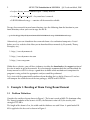
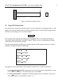
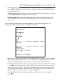
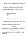
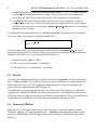
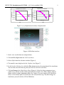
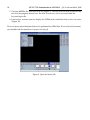
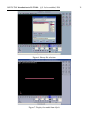
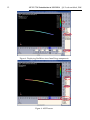
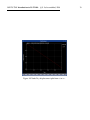
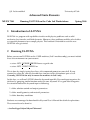
c Leelavanichkul
S.
University of Utah
Advanced Finite Elements
ME EN 7540
Running LS-DYNA on the Cade Lab Workstations
Spring 2006
1 Introduction to LS-DYNA
LS-DYNA is a program with capabilities to solve multi-physics problems such as solid
mechanics, heat transfer, and fluid dynamics. Moreover, these problems could be solved either
as separated phenomena or as couple physics. This handout is intended to assist the new
LS-DYNA user get started.
2 Running LS-DYNA
Before you can run LS-DYNA on the CADE machines (Lab 1 machines only), you must include
these two environment on your account.
• setenv LSTC LICENSE SERVER license.eng.utah.edu
• setenv LSTC CLIENT DEBUG on
This is done by simply typing these lines at the command prompt on your shell. If your
account has .cshrc file, you can also add these two lines to the environment part as well.
Currently, LS-DYNA can only be run on the machines in Lab 1 only.
In this class, we will run LS-DYNA from the keyword input file. Keyword input organizes the
database by grouping similar function under the same keyword. It is a good idea to organize
the structure block of the keyword input as following:
1. define solution control and output parameters
2. define model geometry and material parameters
3. define boundary conditions
Students are encouraged to download the Keyword User’s Manual for detailed explanations.
These manuals can be found at:
>/usr/local/apps/lsdyna/lsdyna970/manual
c Leelavanichkul, 2006
ME EN 7540 Introduction to LS-DYNA S.
2
• ls-dyna theory manual 2005-beta.pdf → theory manual.
• ls-dyna 970 manual k.pdf → keyword user’s manual.
• LSDYNAManuals.tar.gz → contains all the manuals available.
To copy these manuals to your home directory, type the following from the location in your
home directory where you want to copy the file to:
> cp /usr/local/apps/lsdyna/lsdyna970/manual/LSDYNAManuals.tar.gz LSDYNAManuals.tar.gz
Alternatively, you can also obtain these manuals from a few authorized companies. Listed
below are a few websites that allow you to download these manuals (ie, Keywords, Theory,
Examples, etc.).
1. http://www.dynamore.de
2. http://www.dynamax-inc.com
3. http://www.arup.com
Within these websites, you will have to browse to either the download or the support section of
the sites in order to get to the manuals. It is also strongly recommended that you download the
theory manual as well. It is always a good ideas to know which methods or assumptions the
program is using so that the appropriate analyzes could be performed.
Let’s start with the geometrically nonlinear beam bending that we did in Homework 5 and we
will compare the results between the two packages, ANSYS and LS-DYNA.
3
3.1
Example 1: Bending of Beam Using Beam Element
Problem Definition
Consider the cantilever beam shown in Figure 1. The beam is made of 6061-T6 aluminum alloy.
The Young’s modulus of the beam is 69 GPa, the Poission’s ratio is 0.33, the tensile yield
strength is 275 MPa.
The length of the beam is 5 m, the width and the thickness are coth 10 cm. A point load of 10
kN is applied at the free end as shown in Figure 1.
c Leelavanichkul, 2006
ME EN 7540 Introduction to LS-DYNA S.
3
P
h
l
b
Figure 1: Sketch of cantilever beam.
3.2
Input File Preparation
We will consider 4 element and 5 node points. To start writing the keyword input file, we will
follow the layout mentioned in the previous section but first we need to tell the program that
this file we are creating is in a ”keyword” format.
*keyword
The first line of the input file must begin with *keyword. This sets the format of the file as
”keyword” format instead of ”structured” format. From here on, any commands that begin
with asterisk are considered keywords.
The first structure block will define the solution control and the output parameters. For this
problem, this block is defined as following:
*control implicit general
1,0.005
*control termination
1
*database binary d3plot
0.005
*database history node
1,2,3,4,5
*database nodout
1
The group of values listed under each keyword is referred to as ”card” by LS-DYNA.
• *control implicit general This command is used to set the analysis to implicit by set the
first value in the card to 1. The initial time step is set to 0.005,
• *control termination It is important to tell the program when to terminate. In our case,
the computation is set to terminate at time = 1 s,
4
c Leelavanichkul, 2006
ME EN 7540 Introduction to LS-DYNA S.
• *database binary d3plot This keyword saves the binary results in a file called d3plot at
every 0.005 s. This binary results can later be viewed in a program called LSPrePost that
we will later discuss,
• *database history node This keyword write the output for the listed nodes in its card into
a binary history file. In our program, this file is nodout,
• *database nodout Our history file containing nodal data for the selected nodes in the
above keyword. Value of 1 in the card tells the program to only output the data at time
step = 1 s.
In the second input block defines the model geometry and the material properties. The
following keywords and their cards are needed for this model:
*part
aluminum beam
1,1,1
*section beam
1,2
area,Iyy ,Ixx ,J
*mat elastic
1,ρ,E,ν
*node
node 1,x1 , y1 , z1 , translation constraints, rotation
constraints
..
.
node n,xn , yn , zn , translation constraints, rotation
constraints
*element beam
element 1,1,n1a , n1b ,6,0,0,0,0,2
..
.
element n,1,nna , nnb ,6,0,0,0,0,2
• *part The first card of this keyword is the heading and here we called our part ”aluminum
beam”. The second card is the part ID, section ID, material ID, respectively. These are the
IDs that are used through the code to refer to the part, section, and the material,
• *section beam This keyword defines the cross section of the beam. The first card contains
section ID and element formulation. The available element formulation options are listed
in the Keyword User’s Manual. You will have to look this one up and explain to yourself
which element formulation is being used here. The second card of this keyword is more
obvious. It takes the value of area,Iyy ,Ixx ,and J is this order,
• *mat elastic Material density, Young’s modulus, and Possion’s ratio are assigned to
material ID 1,
c Leelavanichkul, 2006
ME EN 7540 Introduction to LS-DYNA S.
5
• *node Similarly to ANSYS, you define the node number and give it its global coordinate
location. The constraints options values are listed in the Keyword User’s Manual, and these
are for you to look them up by yourself,
• *element beam This keyword create element from 2 nodes, na and nb . The second term in
the card specify which part ID this element is using. All the zeros represent no constraints
released in any DOF. The last entry in this card set the coordinate system to local.
Our last block structure for the keyword input file will be the loads and the boundary
conditions. First we will define the load as a concentrated load, then we will define the load
curve.
*load node point
node,direction, load ID, scaling factor
*define curve
load ID
0,0
1,-10e3
• *load node point This keyword applies the concentrated load to the chosen node (first
value in the card). The direction takes the value of 1,2,3 for x,y,z-direction, respectively.
Third term is the load ID, which must be unique for each load,
• *define curve First card in this keyword contain the corresponding load ID to the above
keyword. The second card is the first coordinate of the load curve (time, load). In this case
it is (0,0). The third card is the second point (1,-10000), which represent the final load at
the final time step that we have defined in the first block.
To run LS-DYNA, the following line is entered at the command prompt
>lsdyna i=filename.k
Now putting this together we have the file ex01.k, which is illustrated in the Appendix 1. At
command prompt in your directory, type: >lsdyna i=ex01.k to run the simulation. Once the
computation is done, we will have two result files, nodal results (nodout) and the binary file
(d3plot). nodout can be viewed in any text editors or spreadsheet programs but d3plot can only
be viewed via LSPrePost in the CADE lab. LSPrePost is an advanced program with pre/post
processor for LS-DYNA. It allows you to view results from the computations. It can display
contour plots, display deformations, animate the simulations, etc. For this example, we will not
use LSPrePost since the d3plot doesn’t generate results that we cannot view from the nodal
history file nodout.
c Leelavanichkul, 2006
ME EN 7540 Introduction to LS-DYNA S.
6
3.3
Results
Now, let’s compare the results obtained here to the one from ANSYS. The x and y-displacement
of each node are shown in Figure 2.
y-displacement at each node
0.00E+00
-1.00E-02 0
2
4
6
-2.00E-02
-3.00E-02
LS-DYNA
-4.00E-02
ANSYS
-5.00E-02
-6.00E-02
-7.00E-02
y-displcement (m)
x-displcement (m)
x-displacement at each node
0.00E+00
-1.00E-01 0
2
4
6
-2.00E-01
-3.00E-01
LS-DYNA
-4.00E-01
ANSYS
-5.00E-01
-6.00E-01
-7.00E-01
-8.00E-01
node number
(a)
node number
(b)
Figure 2: (a) nodal x-displacement and (b) nodal y-displacement.
There are some differences in the nodal results. This could be due to several reasons. One thing
that you could check is to consult the Theory Manual of these two packages and see the
differences in technique that each uses. The card in the *section beam specifies certain type of
beam technique used. Can you tell which one? (Hint: Look up the keywords in Keyword User’s
Manual)
It should be pointed out that the values in each card shown for each keyword here are only
what are needed for this problem. In different models, some cards may require more values to
be entered. It is strongly suggested that you have the ls-dyna 970 manual k.pdf handy when you
write the keyword input file. This file is tricky to write and there are many ways you can
manipulate it for different analysis. You will notice in the second example that some keywords
are the same but contain different numbers of entries in their cards.
4
4.1
Example 2: Bending of Beam Using Shell Element
Problem Definition
Now the same problem as in Example 1 is solved using the shell element. We will use 20
elements along the length of the beam and 4 elements along the height of the beam. The DOF at
the left end is constraint in all direction including rotations. A point load is applied at the top
right corner of the beam.
c Leelavanichkul, 2006
ME EN 7540 Introduction to LS-DYNA S.
4.2
7
Input File Preparation
The first block of the keyword input remains the same as the previous example. On the other
hand, the model geometry and material properties block is changed.
*part
aluminum beam
1,1,1
*section shell
1,2
t1 , t2 , t3 , t4
*mat elastic
1,ρ,E,ν
*node
node 1,x1 , y1 , z1
..
.
node n,xn , yn , zn *element shell
element 1,1,n1a , n1b , n1c , n1d
..
.
element n,1,nna , nnb , nnc , nnd
*set node list
1 47,50,53,56,59,62,65,68
71,74,77,80,83,86,89,92
95,98,101,104,24
*set node list
2
1,26,46,47,48
• *part Same explanation as in Example 1,
• *section shell This keyword defines the cross section of the shell. The first card contains
section ID and element formulation. The available element formulation options are listed
in the Keyword User’s Manual. You will have to look this one up and decide for yourself
which element formulation is appropriate for your analysis. The second card of this
keyword takes the thickness value at each of the 4 nodes that form the shell element,
• *mat elastic Material density, Young’s modulus, and Possion’s ratio are assigned to
material ID 1,
• *node Similarly to ANSYS, you define the node number and give it its global coordinate
location. The constraints options are skipped in this example. Instead, an alternative way
to define the boundary conditions is used later in the code,
c Leelavanichkul, 2006
ME EN 7540 Introduction to LS-DYNA S.
8
• *element shell This keyword create element from 4 nodes, n1 to n4 . The second term in
the card specify which part ID of this element. All the zeros represent no constraints
released in any DOF. The last entry in this card set the coordinate system to local,
• *set node list This keyword put number of nodes into a set. Card option 1 is the set
number, while card 2,3,4... contains the nodes that are assigned to this set. Only 8 nodes
are allowed per card. Set 1 is used for the *database history node and Set 2 is used for the
constraint in this example.
Last block of the keyword input file is the boundary conditions and load curves. Everything
here is the same as in Example 1 except the additional of
*boundary spc set
2,0,1,1,1,1,1,1
and the location of the load is also changed to node 22 instead. *boundary spc set sets the
boundary of the selected set. The first value is in its card is the selected set number, follows by
coordinate ID, DOF in x,y,z, and the rotation DOF about x,y,z.
• coordinate ID: 0 - global, 1 - local,
• DOF in x,y,z: 0 - no constraint, 1 - constraint,
• DOF about x,y,z: 0 - no constraint, 1 - constraint.
4.3
Results
The whole keyword input file of this example is illustrated in Appendix 2. To run this analysis,
type: >lsdyna = ex02.k. Once again, the results are save to 2 files that we specified in the first
block of the code. First, let’s take a look at the nodal history file (nodout) and compare the
results to the one obtained from ANSYS (Figure 3).
The differences are very noticeable this time. Keep in mind that shell element is used in this
simulation. In ANSYS, PLANE42 (2-D 4 node) element is used. You should consult the Theory
Manuals of these two software package to see elements are formulated. There are possibly other
explanations for the differences in results that you should try to think of as well.
4.4
Running LSPrePost
Since we have a 2-D model instead of just a line, this time we can make a good use out of
LSPrePost program. To start the program, type: >lsprepost at the command prompt in your
directory, and LSPrePost GUI will appear on your screen (Figure 4). Follow the steps listed
below to
c Leelavanichkul, 2006
ME EN 7540 Introduction to LS-DYNA S.
x-displacement vs distance
y-displacement vs distance
1
2
3
4
5
0.00E+00
-1.00E-02 0
6
-2.00E-01
-3.00E-01
LS-DYNA
-4.00E-01
ANSYS
-5.00E-01
-6.00E-01
x-displacement (m)
y-displacement (m)
0.00E+00
-1.00E-01 0
9
1
2
3
4
5
6
-2.00E-02
-3.00E-02
LS-DYNA
-4.00E-02
ANSYS
-5.00E-02
-6.00E-02
-7.00E-02
-7.00E-01
-8.00E-02
-8.00E-01
distance (m)
distance (m)
(a)
(b)
Figure 3: (a) y-displacement and (b) x-displacement.
Figure 4: LSPrePost interface.
1. load a view results from our computations:
2. Click on File>Open from the Pull Down Menu.
3. Select d3plot from the selection window (Figure 6).
4. The model is now displayed in the Graphics Area (Figure 7).
5. In the Interface Working Area, click the Play button to play the animation of the simulation.
You can also select the time step that you wish to view the result here.
6. Click on Fcomp in the Main Button Menu (Figure 8). Select the fringe component you
which to see and the results will be updated in the Graphics Area. For example, click on
Stress and then choose von mises stress, the Graphics Area now displays the Von Mises
Stress as the contour plot over the beam at the selected time step. Try other fringes to
familiarize yourself with the GUI of LSPrePost.
10
c Leelavanichkul, 2006
ME EN 7540 Introduction to LS-DYNA S.
7. Click on ASCII in the Main Button Menu (Figure 9). The files that end with asterisk are the
one that the program already have the data. In our case, nodout is created from the
keyword input file.
8. Load nodout, and now you can display the XYPlot of the nodal data that we have in nodout
(Figure 10).
There are many other functions that can be performed by LSPrePost. If you wish to learn more,
you should read the tutorials in ls-prepost-tutorial.pdf
Figure 5: Open the binary file.
c Leelavanichkul, 2006
ME EN 7540 Introduction to LS-DYNA S.
Figure 6: Binary file selection.
Figure 7: Display the model from d3plot.
11
12
c Leelavanichkul, 2006
ME EN 7540 Introduction to LS-DYNA S.
Figure 8: Displaying Von Mises stress from Fringe components.
Figure 9: ASCII screen.
c Leelavanichkul, 2006
ME EN 7540 Introduction to LS-DYNA S.
Figure 10: Node 24 y-displacement plot from t0 to t201 .
13
14
c Leelavanichkul, 2006
ME EN 7540 Introduction to LS-DYNA S.
Appendix 1: Keyword input listing for ex01.k
*keyword
*title
ex01.k - cantilever beam
$$$$$$$$$$$$$$$$$$$$$$$$$$$$$$$$$$$$$$$$$$$$$$$
$define solution control and output parameters
$$$$$$$$$$$$$$$$$$$$$$$$$$$$$$$$$$$$$$$$$$$$$$$
*control_implicit_general
1,0.005
*control_termination
1
*database_binary_d3plot
0.005
*database_history_node
1,2,3,4,5
*database_nodout
1
$$$$$$$$$$$$$$$$$$$$$$$$$$$$$$$$$$$$$$$$$$$$$$$
$define model geometry and material parameters
$$$$$$$$$$$$$$$$$$$$$$$$$$$$$$$$$$$$$$$$$$$$$$$
*part
aluminum beam
1,1,1
*section_beam
1,2
0.01,8.3333e-6,8.3333e-6,1.4083e-5
*mat_elastic
1,2710,69e9,0.33
*node
1,0,0,0,7,7
2,1.25,0,0,0,0
3,2.5,0,0,0,0
4,3.75,0,0,0,0
5,5,0,0,0,0
6,2.5,2.5,0,0,0
*element_beam
1,1,1,2,6,0,0,0,0,2
2,1,2,3,6,0,0,0,0,2
3,1,3,4,6,0,0,0,0,2
4,1,4,5,6,0,0,0,0,2
$$$$$$$$$$$$$$$$$$$$$$$$$$$$$$$$$$$$$$$$$$$$$$$
$define boundary conditions
$$$$$$$$$$$$$$$$$$$$$$$$$$$$$$$$$$$$$$$$$$$$$$$
*load_node_point
5,2,1,1
*define_curve
1
0,0
1,-10e3
*end
c Leelavanichkul, 2006
ME EN 7540 Introduction to LS-DYNA S.
Appendix 2: Keyword input listing for ex02.k
*keyword
*title
ex02.k - nonlinear cantilever beam using shell element
$$$$$$$$$$$$$$$$$$$$$$$$$$$$$$$$$$$$$$$$$$$$$$$
$define solution control and output parameters
$$$$$$$$$$$$$$$$$$$$$$$$$$$$$$$$$$$$$$$$$$$$$$$
*control_implicit_general
1,0.005
*control_termination
1
*database_nodout
1
*database_history_node_set
1
*database_binary_d3plot
0.005
$$$$$$$$$$$$$$$$$$$$$$$$$$$$$$$$$$$$$$$$$$$$$$$
$define model geometry and material parameters
$$$$$$$$$$$$$$$$$$$$$$$$$$$$$$$$$$$$$$$$$$$$$$$
*part
aluminum beam
1,1,1
*section_shell
1,2
0.1,0.1,0.1,0.1
*mat_elastic
1,2710,69e9,0.33
*node
1,0,0,0
2,5,0,0
3,0.25,0,0
4,0.5,0,0
5,0.75,0,0
6,1,0,0
7,1.25,0,0
8,1.5,0,0
9,1.75,0,0
10,2,0,0
11,2.25,0,0
12,2.5,0,0
13,2.75,0,0
14,3,0,0
15,3.25,0,0
16,3.5,0,0
17,3.75,0,0
18,4,0,0
19,4.25,0,0
20,4.5,0,0
21,4.75,0,0
22,5,0.1,0
23,5,2.50E-02,0
24,5,5.00E-02,0
25,5,7.50E-02,0
26,0,0.1,0
27,4.75,0.1,0
28,4.5,0.1,0
29,4.25,0.1,0
30,4,0.1,0
31,3.75,0.1,0
32,3.5,0.1,0
33,3.25,0.1,0
34,3,0.1,0
35,2.75,0.1,0
36,2.5,0.1,0
37,2.25,0.1,0
15
16
38,2,0.1,0
39,1.75,0.1,0
40,1.5,0.1,0
41,1.25,0.1,0
42,1,0.1,0
43,0.75,0.1,0
44,0.5,0.1,0
45,0.25,0.1,0
46,0,7.50E-02,0
47,0,5.00E-02,0
48,0,2.50E-02,0
49,0.25,2.50E-02,0
50,0.25,5.00E-02,0
51,0.25,7.50E-02,0
52,0.5,2.50E-02,0
53,0.5,5.00E-02,0
54,0.5,7.50E-02,0
55,0.75,2.50E-02,0
56,0.75,5.00E-02,0
57,0.75,7.50E-02,0
58,1,2.50E-02,0
59,1,5.00E-02,0
60,1,7.50E-02,0
61,1.25,2.50E-02,0
62,1.25,5.00E-02,0
63,1.25,7.50E-02,0
64,1.5,2.50E-02,0
65,1.5,5.00E-02,0
66,1.5,7.50E-02,0
67,1.75,2.50E-02,0
68,1.75,5.00E-02,0
69,1.75,7.50E-02,0
70,2,2.50E-02,0
71,2,5.00E-02,0
72,2,7.50E-02,0
73,2.25,2.50E-02,0
74,2.25,5.00E-02,0
75,2.25,7.50E-02,0
76,2.5,2.50E-02,0
77,2.5,5.00E-02,0
78,2.5,7.50E-02,0
79,2.75,2.50E-02,0
80,2.75,5.00E-02,0
81,2.75,7.50E-02,0
82,3,2.50E-02,0
83,3,5.00E-02,0
84,3,7.50E-02,0
85,3.25,2.50E-02,0
86,3.25,5.00E-02,0
87,3.25,7.50E-02,0
88,3.5,2.50E-02,0
89,3.5,5.00E-02,0
90,3.5,7.50E-02,0
91,3.75,2.50E-02,0
92,3.75,5.00E-02,0
93,3.75,7.50E-02,0
94,4,2.50E-02,0
95,4,5.00E-02,0
96,4,7.50E-02,0
97,4.25,2.50E-02,0
98,4.25,5.00E-02,0
99,4.25,7.50E-02,0
100,4.5,2.50E-02,0
101,4.5,5.00E-02,0
102,4.5,7.50E-02,0
103,4.75,2.50E-02,0
104,4.75,5.00E-02,0
105,4.75,7.50E-02,0
c Leelavanichkul, 2006
ME EN 7540 Introduction to LS-DYNA S.
c Leelavanichkul, 2006
ME EN 7540 Introduction to LS-DYNA S.
*set_node_list
1
47,50,53,56,59,62,65,68
71,74,77,80,83,86,89,92
95,98,101,104,24
*set_node_list
2
1,26,46,47,48
*element_shell
1,1,1,3,49,48
2,1,3,4,52,49
3,1,4,5,55,52
4,1,5,6,58,55
5,1,6,7,61,58
6,1,7,8,64,61
7,1,8,9,67,64
8,1,9,10,70,67
9,1,10,11,73,70
10,1,11,12,76,73
11,1,12,13,79,76
12,1,13,14,82,79
13,1,14,15,85,82
14,1,15,16,88,85
15,1,16,17,91,88
16,1,17,18,94,91
17,1,18,19,97,94
18,1,19,20,100,97
19,1,20,21,103,100
20,1,21,2,23,103
21,1,48,49,50,47
22,1,49,52,53,50
23,1,52,55,56,53
24,1,55,58,59,56
25,1,58,61,62,59
26,1,61,64,65,62
27,1,64,67,68,65
28,1,67,70,71,68
29,1,70,73,74,71
30,1,73,76,77,74
31,1,76,79,80,77
32,1,79,82,83,80
33,1,82,85,86,83
34,1,85,88,89,86
35,1,88,91,92,89
36,1,91,94,95,92
37,1,94,97,98,95
38,1,97,100,101,98
39,1,100,103,104,101
40,1,103,23,24,104
41,1,47,50,51,46
42,1,50,53,54,51
43,1,53,56,57,54
44,1,56,59,60,57
45,1,59,62,63,60
46,1,62,65,66,63
47,1,65,68,69,66
48,1,68,71,72,69
49,1,71,74,75,72
50,1,74,77,78,75
51,1,77,80,81,78
52,1,80,83,84,81
53,1,83,86,87,84
54,1,86,89,90,87
55,1,89,92,93,90
56,1,92,95,96,93
57,1,95,98,99,96
58,1,98,101,102,99
59,1,101,104,105,102
17
18
c Leelavanichkul, 2006
ME EN 7540 Introduction to LS-DYNA S.
60,1,104,24,25,105
61,1,46,51,45,26
62,1,51,54,44,45
63,1,54,57,43,44
64,1,57,60,42,43
65,1,60,63,41,42
66,1,63,66,40,41
67,1,66,69,39,40
68,1,69,72,38,39
69,1,72,75,37,38
70,1,75,78,36,37
71,1,78,81,35,36
72,1,81,84,34,35
73,1,84,87,33,34
74,1,87,90,32,33
75,1,90,93,31,32
76,1,93,96,30,31
77,1,96,99,29,30
78,1,99,102,28,29
79,1,102,105,27,28
80,1,105,25,22,27
$$$$$$$$$$$$$$$$$$$$$$$$$$$$$$$$$$$$$$$$$$$$$$$
$define boundary conditions
$$$$$$$$$$$$$$$$$$$$$$$$$$$$$$$$$$$$$$$$$$$$$$$
*boundary_spc_set
2,0,1,1,1,1,1,1
*load_node_point
22,2,1,1
*define_curve
1
0,0
1,-10e3
*end