Download GEOCRACK User`s Manual - Cornell Fracture Group

Simulations on Statistical Representations of
Polycrystals using FRANC2D/L
Polycrystal User's Guide
December 2001
Erin Iesulauro and Ketan Dohdia
Cornell University • Ithaca, New York
Page ii
Table of Contents
Table of Contents
Introduction....................................................................................................................3
Outline of Procedure .....................................................................................................3
Grain Geometry .......................................................................................................3
Voronoi Tessellation ................................................................................................3
Grain Material .........................................................................................................4
Grain Boundaries.....................................................................................................4
Grain Boundary Property Assignment.................................................................4
Cohesive Zone Model ..........................................................................................4
Coupled Cohesive Zone Model ...........................................................................5
Unloading of the Coupled Cohesive Zone Model..........................................6
Interface Elements ...............................................................................................7
Creating Statistical Samples of Polycrystals for FRANC2D/L .................................9
Grain Geometry ...................................................................................................9
Particle Insertion ..................................................................................................9
Meshing ...............................................................................................................10
Assigning Grain Material Properties ............................................................11
Assigning Particle Material Properties.........................................................11
Defining Cohesive Zone Models .........................................................................12
Input *.inp File Format ........................................................................................12
FRANC2D/L Example...................................................................................................16
Building an Initial Geometry and Mesh ..............................................................16
Performing a FRANC2D/L Simulation ...............................................................17
Defining the Problem Type ............................................................................18
Boundary Conditions: Fixities.......................................................................18
Inserting Interface Elements..........................................................................18
Setting the Material Properties......................................................................18
Applied Displacements ..................................................................................18
Perform Analysis............................................................................................18
Post-Processing .............................................................................................19
Acknowledgments ..........................................................................................................20
Bibliography ...................................................................................................................21
Index................................................................................................................................23
FRANC2D/L Short User's Guide
Outline of Procedure
Page 3
Introduction
After examining the microstructure of the AA 7075-T6, a meso-scale representation was
created on which to perform simulations and to study the microstructural influences on
crack initiation. The process of creating a meso-scale model with discrete grains
represented was broken down into three stages: creating a grain geometry, determination
of material model and properties for the grains, and determination of how to represent the
grain boundaries to allow the initiation of cracks.
Outline of Procedure
Grain Geometry
The representation of the grain geometry could either be done to match a single observed
polycrystal sample or to represent the average geometry seen over many samples. It was
decided to represent the geometry in an average sense. The polycrystal samples
generated statistically match observation in terms of quantities such as average grain size
and aspect ratio. However, samples won't exactly match any observed geometry. For
this work, the Voronoi tessellation was chosen as the method by which to create the grain
geometries.
Voronoi Tessellation
Voronoi tessellation begins from a random distribution of nuclei. Lines are generated
connecting a nucleus to its nearest neighbors. These lines are then perpendicularly
bisected to create the edges of a polygon. Each nucleus then defines a polygon within
which all points are closer to the nucleus than to any other. This process best represents
the initial forming of the grains from dendrite sites within a melt with isotropic growth
rates [Arawde].
This particular choice represents the initial polycrystal structure or annealed structure
well. However, Voronoi tessellations do not capture the distortion of the grains due to
processing such as rolling. Since this work was done in 2D it was determined that this
would be a good tessellation with which to test modeling choices and software
capabilities. Ongoing work is looking at modifications to the Voronoi tessellation as well
as other tessellation methods that will better represent the rolled grain structure.
Current modeling has been expanded to consider the discrete modeling of sub-grain sized
particles. Particles well below the size of the grains are considered to be smeared out and
represented through the grain material properties.
FRANC2D/L Short User's Guide
Page 4
Outline of Procedure
Grain Material
Once the geometry is in place material properties are assigned to each grain. Current
material model options include elastic, isotropic; elastic, orthotropic; isotropic, elasticplastic; and orthotropic, elastic-plastic. Details concerning the plasticity implementation
can be found in James. See the FRANC2D/L User’s Guide for the necessary parameters.
For the chosen material model each grain is assigned values of the appropriate
parameters.
Grain Boundaries
In a polycrystal there are many mechanisms that can lead to the initiation of microcracks. For example, fatigue leads to the formation of slip bands within grains, which
can lead to shear cracks. Also, a corrosive environment can lead to the failure of grain
boundaries due to oxygen embrittlement. The simulations conducted focus on grain
boundary decohesion as the primary source of localized damage. To allow decohesion to
occur naturally grain boundaries were modeled using cohesive zone models. The
following discusses the theory and implementation of cohesive zone models.
Grain Boundary Property Assignment
Grain boundaries naturally arise in polycrystals due to the lattice mismatch between
adjacent grains. This region of disordered atoms acts differently than the regular lattices
of the adjacent grains. Therefore, we describe the grain boundary with its own
constitutive relationship, separate from the bulk grain material. A cohesive zone model
has been chosen for this purpose to describe the strength and toughness of the grain
boundaries. The cohesive zone model also serves as a criterion for initiation of
intergranular cracks. The grain boundaries are allowed to decohere after reaching a
critical normal, shear, or combined transmitted traction, thus gradually initiating a crack.
Once a critical opening is reached a true crack has formed. An advantage of using such a
model is that initial cracks are not arbitrarily introduced at the beginning of a simulation.
Instead, cracks naturally occur due to the heterogeneous stress field throughout the
sample caused by the geometry and variations in properties.
Cohesive Zone Model
In theory, the stress at a crack tip goes to infinity creating a stress singularity. However,
in practice materials, especially metals, have a yield stress at which they begin to deform
plastically negating the singularity. This leads to the area around the crack tip called the
crack tip plastic zone. The stress in the plastic zone can only reach the yield stress. The
additional stress due to the singularity must still be carried by the material. Several
methods have been developed to determine the extent of the plastic zone and account for
FRANC2D/L Short User's Guide
Outline of Procedure
Page 5
the stress beyond the yield stress. These include the Irwin’s plastic zone correction and
the strip yield models developed first by Dugdale and Barenblatt .
Dugdale considered a fictitious crack tip a distance ρ ahead of the actual crack tip. The
fictitious tip carries a compressive force equal to the yield stress that tends to close the
crack. An application of this approach by Hillerborg is the fictitious crack model or the
cohesive zone model. The cohesive zone model (CZM) assumes that the compressive
force applied in the plastic zone follows a traction-displacement relationship. It is also
assumed that this traction-displacement behavior can be considered a material property
[Broek][Anderson].
In the present case the damage represented by the strain softening portion of the CZM is
used to describe the decohesion of the grain boundaries leading to crack initiation. Also,
the area under the curve represents the critical energy release rate, Gc, to initiate a crack.
The implementations available in FRANC2D/L [James], includes independent normal
and shear cohesive models as well as a coupled model added for this work. The normal
and shear models evaluate the transmitted traction independently of each other. In other
words, the transmitted normal does not influence the amount of shear and vise verse. The
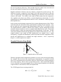
coupled cohesive zone model (CCZM) implemented was adapted from a model
developed by Tvergaard and Hutchinson, where the normal and shear components of the
traction and displacement are combined into single measures, τ and λ, respectively
(Figure 1), so that responses are coupled.
Coupled Cohesive Zone Model
Traction, t
tp
kn
Gc
Figure 1: Coupled cohesive zone
1 model
Relative Displacement, λ
With the segregated models implemented problems can arise under mixed-mode loading.
For example, since the shear and normal operate independently it is possible for shear
forces to be transmitted across an interface while no normal traction is being transmitted
due to large opening. This of course is physically incorrect. Since mixed mode loading
is to be expected in polycrystal samples due to inclined grain boundaries the following
coupled cohesive zone model (CCZM) was implemented.
The CCZM begins from a traction potential, Φ.
Φ(δ n , δ t ) = δ nc ∫ t (λ ′)dλ ′
λ
Eqn. 1
FRANC2D/L Short User's Guide
Page 6
Outline of Procedure
Φ is a function of the relative normal, δn, and tangential, δt, displacements between the
faces of the grain boundary. λ is a non-dimensional separation measure for the relative
opening and sliding defined by Eqn. 2. The opening and sliding displacements are
normalized to the relative critical displacement values, δnc and δtc, at which the separation
is considered a true crack in pure Mode I and pure Mode II. When the value of λ reaches
1 this indicates the complete decohesion of the grain boundary and the formation of a true
crack.
⎡⎛ δ
λ = ⎢⎜⎜ nc
⎢⎣⎝ δ n
2
⎞ ⎛ δt
⎟⎟ + ⎜⎜ c
⎠ ⎝δt
⎞
⎟⎟
⎠
2
⎤
⎥
⎥⎦
1/ 2
Eqn. 2
For a given relative displacement between two grains the combined traction, τ,
transmitted across the grain boundary can be determined from the CCZM. The combined
traction can then be decomposed into normal, Tn, and shear, Tt, components by
differentiating Φ with respect to δn and δt according to Eqn. 3 and Eqn. 4 respectively.
Tn =
∂Φ t (λ ) δ n
=
∂δ n
λ δ nc
∂Φ t (λ ) δ nc δ t
=
Tt =
∂δ t
λ δ tc δ tc
Eqn. 3
Eqn. 4
The CCZM parameters have the following physical implications. The initial stiffness, kn,
represents the elastic response of the grain boundary. Since the grain boundaries are
consider to be stiffer than the bulk grain material kn is set to a high value. The coupled
value of tp relates to the peak normal strength, tpn, and peak shear strength, tpn, according
to Eqn. 5 and Eqn. 6 respectively. Whether plane stress or plane strain is assumed will
vary the value of the coupled peak traction, tp, relative to the bulk yield stress. For plain
strain tp is considered to be three to five times the yield stress. For plane stress the value
is only one to one and a half time the yield stress. For the parametric study the value of tp
is set to observe the influence of the relative values. After the peak traction is reached
atomic bonds begin to break allowing the faces to separate. This portion is considered
the softening of the grain boundary. At a specific distance the opposing face no longer
exert attractive forces on each other resulting in a true crack. This corresponds to λ = 1.
t p = T pn
Eqn. 5
t p = δ ncT pt
Eqn. 6
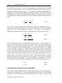
Unloading of the Coupled Cohesive Zone Model
Since cyclic loading conditions will be used, the unloading of the CCZM must be
considered and implemented. Two possible unloading paths considered were unloading
according to the initial stiffness and unloading back to the origin. Both physical
FRANC2D/L Short User's Guide
Outline of Procedure
Page 7
implications of the unloading paths and numerical difficulties were considered before
choosing to unload to the origin.
tp
tp
1
(a)
λ
1
(b)
λ
Figure 2: (a) Unloading according to the initial stifness. (b) Unloading back to the
origin
Unloading according to the initial stiffness allows for plastic deformation in the grain
boundary to occur. Once the interface has returned to zero traction the displacement is
not necessarily zero. This reflects such theories as crack closure. However, this
approach causes implementation problems. When the FRANC2D/L software calculates
the stiffness matrix for the model a tangent stiffness is determined for each element. For
the interface elements the secant stiffness is calculated instead. The solution technique
used requires the stiffness matrix to be positive definite. Therefore the negative slope of
the softening portion of the curve is not acceptable. To compensate for this the secant
stiffness is calculated instead, which still captures the softening of the stiffness matrix.
Keeping this in mind, it follows that by unloading according to the initial stiffness would
result in an increase in stiffness of the interface upon unloading and reloading.
Unloading back to the origin does result in a fully closed interface. However, the
interface instead sees damage through maintaining a lower stiffness value upon
reloading. This also removes several difficulties that would be experienced in
implementation. For this reason unloading back to the origin was implemented.
Interface Elements
A convenient method for implementing the CZMs is through zero thickness interface or
joint elements. The 6 noded interface element (Figure 3) implemented here creates
traction forces as a function of the displacement prescribed by the CZM. The displaced
location of the centerline of the element is determined from the nodal positions. From
this the relative displacements of node pairs are determined and interpolated to the Gauss
integration points. At each of the integration points the traction is then computed from
the CZM specified and integrated to determine the work equivalent nodal loads. The
stiffness can also be determined from the CZM based on the relative displacement
[Wawryznek][Bittencourt]. A tutorial for using interface elements in FRANC2D/L
FRANC2D/L Short User's Guide
Page 8
Outline of Procedure
simulations is included in Appendix A of Iesulauro or in the FRANC2D/L User’s Guide
version 2.0.
x x x x x
Figure 3: 6-noded interface element and location of intergration points
FRANC2D/L Short User's Guide
Creating Statistical Samples of Polycrystals
Page 9
Creating Statistical Samples of
Polycrystals for FRANC2D/L
The *.inp file for Franc2D/L contains mesh information as well as material definitions
and assignments to each element. Traditionally creating an *.inp is done using CASCA.
This is an independent modeling and meshing program. A description of this tool is
available in the FRANC2D and FRANC2D/L Manuals.
The statistical creation of polycrystal models and the corresponding *.inp however, is not
done through CASCA. Instead a series of Matlab functions were created to statistically
generate polycrystal geometries and distributions of particles and as well as distributions
of material properties.
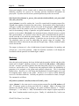
The follow outlines the steps for creating a polycrystal sample and the corresponding
*.inp file. The next section contains an tutorial including commands for creating a
polycrystal sample.
Grain Geometry
Grain geometries are determined using Voronoi tessellation as described previously. The
process of creating the tessellation has been compiled into a single Matlab script,
DM_tess.
DM_tess(‘jobname’,dim,num,seed,seed)
‘jobname’ is a string indicating the name to be used for the output file. DM_tess calls a
fortran program Vor.f that creates the tessellation. This program produces a square
sample. Dim is the dimension of the square to be tessellated. Vor.f requires either the
number of grains to be created or the average grain size. DM_tess is currently set to
accept the number of grains, num. FRANC2D/L is capable of reading up to 500 material
definitions. This includes grain materials as well as cohesive zone model definitions.
This should be taken into account when determining the number of grains to create.
Finally, 2 random number seeds are needed.
The output is the file jobname.tess. This contains the tessellation information. To view
the tessellation use DM_plottess(‘jobname’). There are also several intermediate files
that are generated but are not necessary for future steps.
Particle Insertion
FRANC2D/L Short User's Guide
Page 10
Tutorial
Polycrystal samples can be created with or without the inclusion of particles. The
following describes the process for inserting particles distributed throughout the
polycrystal. If you do not wish to have particles present skip to the next section.
DM_ParticleList(‘jobname’,n_parts,n_sides,ratio,threshold,subdivide_ratio_max,subdi
vide_ratio_min,seed)
Again jobname is used for reading the *.tess file created and for naming output files.
N_parts is the number of particles you wish to have. Each particle will be represented as
a polygon, N_sides is the number of sides to be used for the polygons. Ratio determines
the relative size of the particles to the size of the grains. The rest of the variables are
used for determining overlap of particles and grain boundaries and for preparing the
particles to be meshed. Threshold is the minimum distance allowed between a particle
and a grain boundary. If a particle is closer than the value of threshold then the particle is
moved such that it will touch the grain boundary. This value is also used to determine
the minimum distance between particles. If particles are too close they will be joined.
The subdivide_ratios are used for subdividing the particle edges for meshing. The
subdivisions must be between the min and max*longest edge. Finally a random number
seed is also needed.
The output is jobname.sub, a list of subdivision of particle boundaries for meshing, and
jobname.par, a list of the particles. When the function concludes it will display the
tessellation with the particles in a Matlab figure window.
Meshing
Once the polycrystal geometry has been defined and the particles defined and placed the
model can be meshed. Meshing routines are called from DM_mshtess. DM_mshtess
uses the *.tess and *.par files to generate the mesh along with properties.txt, partprop.txt,
betalist.txt, and hardcurve.txt. Properties.txt and partprop.txt define the distribution of
properties to be assigned to the grains and particles respectively. This is described
further below. Betalist.txt is a file listing the distributions of material angles to be used
for assigning lattice angles to the grains. Hardcurve.txt is used to define hardening
curves for von Mises materials. Currently the particles are modeled as elastic, isotropic.
The command is as follows.
DM_mshtess(‘jobname’,mat,dim,nseed,nseed2,subdiv_ratio)
Again ‘jobname’ is the name used to create previous output files that DM_mshtess will
call. If isotropic grains are being used this file is ignored. Mat is an integer that
indicates the material model to assign to the grains (1-Elastic-Isotropic, 2 – ElasticOrthotropic, 3 – von Mises, 4 – Hill). The dimension of the sample is again requested in
dim. Next 2 random number seeds are given. Finally, if a subdivide file (*.sub) is not
FRANC2D/L Short User's Guide
Creating Statistical Samples of Polycrystals
Page 11
provided the mesh generator using the single value specified by subdiv_ratio. This
determines the density of the mesh.
Assigning Grain Material Properties
The meshing step also assigns material numbers to each element. The material numbers
refer to a defined material model. For each sample a material model is chosen to describe
the grain material. To add statistical variation for the given material model a different set
of parameters can be assigned to each grain throughout the sample.
For each parameter in the material model a mean value and range are read from the
properties.txt file. These values define a uniform distribution of values for the parameter.
Matlab then creates a material definition by selecting values from the uniform
distribution for each parameter. The format of the file is as follows.
E1: mean range std deviation
E2: mean range
E3: mean range
Possion's Ratio: ν1 ν2 ν3
Thickness
Density
KIC: mean range std deviation \\
KIC_inf
σyld1: mean range
σyld2: mean range
σyld3: mean range
If particular values are unnecessary for the chosen model 0’s can be entered as
placeholders.
If von Mises, elastic-plastic material properties are desired for the grains hardcurve.txt
can be used to define a uniform distribution of hardening curves. The file consists of the
yield stress, ultimate stress and a range of variation.
Finally, in the case of orthotropic materials, betalist.txt is necessary. This file contains a
distribution of angles from which each grain is assigned a lattice orientation. The angle
assigned is the angle measured counter-clock wise from the global X-axis to the primary
axis of the lattice. In the Hill case, this is the primary yield stress direction.
Assigning Particle Material Properties
A similar process is followed for defining material models for the particles and assigning
material numbers to the elements within each particle. The particle properties are taken
from the file partprop.txt. Currently particles are defined as elastic, isotropic so the file
format is as follows.
E1: mean range std deviation
FRANC2D/L Short User's Guide
Page 12
Tutorial
Possion's Ratio: ν1 ν2 ν3
Thickness
Density
KIC: mean range std deviation \\
The meshing processing creates several intermediate files. These files include tess.out
and particle,out. The final output is an *.inp file. This file can be read by FRANC2D/L.
Defining Cohesive Zone Models
This *.inp file created at this point is readable by FRANC2D/L; however, it does not
contain any information concerning the grain boundaries or particle-grain interfaces. As
discussed previously these responses are determined by CCZMs. This information can
be entered from within FRANC2D/L. If different parameters are used for each grain
boundary it is more efficient to define the models before hand. This is done through two
additional Matlab scripts: DM_MultiCZM1 and DM_ParicletCZM.
DM_MultiCZM1(‘jobname’,beta)
DM_MultiCZM1 appends jobname.inp with parameters defining one more more
cohesive zone models corresponding to ranges of angles of misorientation between
grains. To determine the ranges of properties to be assigned by DM_multiCZM1 the file
must be altered to reflect the values. Beta is the angle range for which each CZM to be
defined will be good for. For example, if you want to use 1 CZM for all grain boundaries
delta = 360. If instead delta = 5, then the first CZM will be valid for grain boundaries
with a misorientation angel between 0 and 5 degrees and then next for 6 to 10 degrees
and so forth.
DM_ParticleCZM(‘jobname’)
DM_ParticleCZM again appends jobname.inp with parameters defining a CZM. This
cohesive zone defines the response of the particle-grain interface. The properties are read
from the file Part_czm.txt.
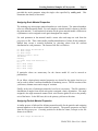
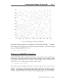
Input *.inp File Format
The steps outlined above result in an .inp input file for FRANC2D/L. The file includes
mesh information as well as material definition and assignments, and cohesive zone
models definitions. The following is an example .inp file for the 16-element block shown
in Figure 4.
65
1
1
2
16
1
1
2.90E+04 2.50E-01 1.00E+00 1.00E+00 1.00E+00
0.00E+00 0.00E+00 0.00E+00 0.00E+00 0.00E+00
1
6
1 53 52 51
2
9
7
1
9
2 51 50 49
3 12 10
FRANC2D/L Short User's Guide
0.00E+00
0.00E+00
Creating Statistical Samples of Polycrystals
3
4
5
6
7
8
9
10
11
12
13
14
15
16
1
2
3
4
5
6
7
8
9
10
11
12
13
14
15
16
17
18
19
20
21
22
23
24
25
26
27
28
29
30
31
32
33
34
35
36
37
38
39
40
41
42
43
44
45
46
1
1
1
1
1
1
1
1
1
1
1
1
1
1
12
3 49
42
4
6
16
5
6
19
8
9
22 11 12
44 14 16
26 15 16
29 18 19
32 21 22
46 24 26
35 25 26
37 28 29
39 31 32
6
4 42
1.500000E+00
1.000000E+00
5.000000E-01
1.750000E+00
1.500000E+00
1.500000E+00
1.250000E+00
1.000000E+00
1.000000E+00
7.500000E-01
5.000000E-01
5.000000E-01
2.500000E-01
1.750000E+00
1.500000E+00
1.500000E+00
1.250000E+00
1.000000E+00
1.000000E+00
7.500000E-01
5.000000E-01
5.000000E-01
2.500000E-01
1.750000E+00
1.500000E+00
1.500000E+00
1.250000E+00
1.000000E+00
1.000000E+00
7.500000E-01
5.000000E-01
5.000000E-01
2.500000E-01
1.750000E+00
1.500000E+00
1.250000E+00
1.000000E+00
7.500000E-01
5.000000E-01
2.500000E-01
2.000000E+00
2.000000E+00
2.000000E+00
2.000000E+00
2.000000E+00
2.000000E+00
48 62 61 60
5 16 14 44
7
9
8 19
10 12 11 22
13 60 59 58
15 26 24 46
17 19 18 29
20 22 21 32
23 58 57 56
25 35 34 64
27 29 28 37
30 32 31 39
33 56 55 65
41 63 54 53
1.750000E+00
1.750000E+00
1.750000E+00
1.500000E+00
1.250000E+00
1.500000E+00
1.500000E+00
1.250000E+00
1.500000E+00
1.500000E+00
1.250000E+00
1.500000E+00
1.500000E+00
1.000000E+00
7.500000E-01
1.000000E+00
1.000000E+00
7.500000E-01
1.000000E+00
1.000000E+00
7.500000E-01
1.000000E+00
1.000000E+00
5.000000E-01
2.500000E-01
5.000000E-01
5.000000E-01
2.500000E-01
5.000000E-01
5.000000E-01
2.500000E-01
5.000000E-01
5.000000E-01
0.000000E+00
0.000000E+00
0.000000E+00
0.000000E+00
0.000000E+00
0.000000E+00
0.000000E+00
1.750000E+00
1.500000E+00
1.250000E+00
1.000000E+00
7.500000E-01
5.000000E-01
Page 13
13
43
17
20
23
45
27
30
33
47
36
38
40
1
Figure 4: 16-element block
FRANC2D/L Short User's Guide
Page 14
47
48
49
50
51
52
53
54
55
56
57
58
59
60
61
62
63
64
65
Tutorial
2.000000E+00
2.500000E-01
5.000000E-01
7.500000E-01
1.000000E+00
1.250000E+00
1.500000E+00
1.750000E+00
0.000000E+00
0.000000E+00
0.000000E+00
0.000000E+00
0.000000E+00
0.000000E+00
0.000000E+00
0.000000E+00
2.000000E+00
2.000000E+00
0.000000E+00
2.500000E-01
2.000000E+00
2.000000E+00
2.000000E+00
2.000000E+00
2.000000E+00
2.000000E+00
2.000000E+00
2.500000E-01
5.000000E-01
7.500000E-01
1.000000E+00
1.250000E+00
1.500000E+00
1.750000E+00
2.000000E+00
2.000000E+00
0.000000E+00
0.000000E+00
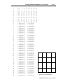
The first line includes the number of nodes, number of elements, number of material
definitions, and the problem type.
This is followed by the material definitions. Materials are numbered according the order
they are listed. Therefore material numbers are not explicitly listed in the .inp file. For
each material definition the first number is the material model (1 – Isotropic, 2 –
Orthotropic, 3 – von Mises, 4 – Hill). The following numbers are the parameters for the
given model.
Next the element conductivities are listed. The element number is followed by the
material definition assigned to that element and the nodes listed in counterclockwise
order.
Next the nodes are listed. Each line contains the node number followed by the X and Y
coordinates.
This would be the end of a typical FRANC2D/L input file. However, information
concerning the von Mises materials and the cohesive zone models are appended to the
end of the file.
The von Mises plasticity model implemented allows hardening to occur. Normally the
hardening curve is defined after opening FRANC2D/L. However, with many materials
defined this becomes inefficient. Therefore the definitions of these curves were
appended to the .inp file following the text string ‘HARDCURVE’. For each von Mises
material defined several lines are appended. The first line indicates the number of points
used to define the curve. Each subsequent line lists the X and Y coordinates of a point on
the curve.
Next the coupled cohesive zone models for the grain boundaries are listed following the
text string ‘multiCZM’. Each coupled cohesive zone model is valid for a range of
FRANC2D/L Short User's Guide
Creating Statistical Samples of Polycrystals
Page 15
misorientations measured across the grain boundary. The angle range is listed first
followed by the model parameters.
Finally, the CCZM used to define the particle-grain interface is listed following the text
spring ‘partCZM’. The format is the same as listed above. However the angle range is
given as 0 360. Currently all particle-grain interfaces follow the same response so just
one model is defined. The angle range is still list however for consistence and the ability
to easily expand in the future.
FRANC2D/L Short User's Guide
Page 16
Tutorial
FRANC2D/L Example
Building an Initial Geometry and Mesh
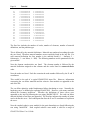
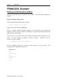
The polycrystal and mesh are generated from Matlab. First create the tessellation as
follows.
DM_tess(‘jobname’,dim,n,nseed)
For this example the following input was used.
DM_tess('tutorial',0.5,100,5492)
Figure 4 shows the results from DM_tess.
This is a simple example therefore particles were not placed in the polycrystal.
Therefore, the next step is to mesh the tessellation, assign grain material properties, and
define cohesive zone models.
The next step is to mesh the polycrystal sample and assign material properties to the
grains. For this example the grains are elastic, isotropic. Therefore, only the
properties.txt file is needed.
DM_mshtess('tutorial',1,0.5,268,542,.1)
For this example hardcurve.txt, betalist.txt, and partprop.txt were not used.
following are the input files properties.txt.
Properties.txt:
72 2 1
0 0
0 0
0.34 0.35 0.35
1
1.0
0.00632 0.0 25
10000000
0 0
0 0
0 0
FRANC2D/L Short User's Guide
The
Creating Statistical Samples of Polycrystals
Page 17
Figure 5: Matlab figure output from DM_tess
Finally, the interface properties are assigned by the following statements. To simplify
this example one CZM will be used for all of the grain boundaries. Therefore the angle
inputted to DM_multiCZM1 will be 360.
DM_multiCZM1('tutorial',360)
Performing a FRANC2D/L Simulation
Start FRANC2D/L with the *.inp file created above. Due to the size of the model it may
be necessary to start the program with extra memory allocated. That is done by calling
the program as shown below. This example is small enough that this command is not
needed. However, for slightly larger models it will be needed.
Franc2dl.exe –mem 25000000
Due to the size of the models it may take a moment for the file to be read. Once the
model is read in there are still several pre-processing steps before the model is ready for
analysis. It is important to follow the procedure in the order listed. Of most importance
is that the interface elements must be placed before applying displacements to the model.
FRANC2D/L Short User's Guide
Page 18
Tutorial
Defining the Problem Type
The problem type is specified under PRE-PROCESS→PROBLEM TYPE menu. Plain
strain is preferred for these models. However, if the grains are defined as Hill materials
then plane stress must be used.
Boundary Conditions: Fixities
Fixities are applied from the PRE-PROCESS→FIXITY menu. For this example the
bottom edge is fixed in the Y-direction. Also the center node is fixed in the X-direction.
The center node is determined by using EL/NO INFO→NODE INFO to determine
which node is closest to the center.
Inserting Interface Elements
At this time, if you did not define an interface model to be used on the grain boundaries
do so now. If this information was appended to the *.inp file then proceed.
As described in the FRANC2D/L version 1.5 user’s guide a feature has been added to
automatically place interface elements along all interfaces. The feature can be assessed
through the PRE-PROCESS→MATERIAL menu. Use the –MAT+ button to move to
any interface model. In the bottom menu will be the button PLACE ALL INTS. Click
on this button. To determine that the interface elements have been placed turn on the
interfaces using the INTRFC: ON/OFF button. The interfaces will appear white while
the other element edges will be orange. If an interface element is present the
corresponding material number will be next to the element. Occasionally this feature
encounters problems. If the program does not return quickly then the function is stuck.
At this point the best advice is to create a new mesh and possibly a new tessellation.
Setting the Material Properties
The grains were assigned material numbers during the meshing process. Therefore no
other action is required here.
Applied Displacements
Finally the displacements are applied. Using loads is discouraged with polycrystal
models since the analysis will likely become unstable.
Apply a unit displacement to the top edge of the model from the PREPROCESS→APPLD DISP menu.
Perform Analysis
FRANC2D/L Short User's Guide
Creating Statistical Samples of Polycrystals
Page 19
Before performing the analysis be sure to save a restart file. This can be done before or
after setting the control parameters. If there is not enough memory the solver will stop
and the program will need to be restarted with more memory. Starting from a restart file
will make this go quicker.
Even if the grains are defined to be elastic, the presence of the interface elements makes
the analysis material non-linear. Therefore select the ANALYSIS→MAT-NONLIN
option.
Select CONTROL PARAM to set up the analysis. The parameters will appear in the
auxiliary window. Using the menu buttons set the option as follows.
Load Sub-Steps
Global Tolerance
Max Iterations :
Load Factor 1 :
Load Factor 2 :
Load Factor 3 :
Load Factor 4 :
Load Factor 5 :
Load Factor 6 :
Appld Dist Factor
Accelerate Iter :
New Analysis :
Current Step :
Final Step
:
Save Frequency
Print Frequency
Increment Method
Anaylsis Mode
Autosave File :
:
:
10
0.1
200
0
0
0
0
0
0
:
0.1e-7
NONE
YES
0
:
:
:
:
10
0
50
FIXED
INCREMENTAL
jobname
Return from this menu. Select ANALYZE ONE to conduct the analysis. Do to the large
number of degrees of freedom the initial set up before the solve actually begins can take a
several minutes. The total solve time for example is about 5 minutes.
Post-Processing
Post-processing options are discussed in the FRANC2D/L User’s Guide. The feature of
note for this simulation is POST-PROCESS→CONTOURS→STRAIN→INT SEPAR.
This shows the separation experienced by the interface elements. This can be useful for
identifying elements that have started to decohere or that have fully decohered.
FRANC2D/L Short User's Guide
Page 20
Bibliography
Acknowledgments
Prof. Anthony Ingraffea (Cornell University) has focused on the goal of developing the
ability to rapidly model discrete crack growth for about fifteen years. FRANC2D/L
represents the work of several generations of students: Prof. Ingraffea modeled discrete
crack growth by changing a mesh described by a deck of computer cards, Victor Sauoma
modeled discrete crack growth on a Tektronix terminal, Walter Gerstle modeled crack
growth on an Evans and Sutherland display, and finally, Paul Wawrzynek (Wash) used a
workstation, started from scratch, and introduced robust data schemes to the engineers
who had come before. Layering has been added by Sudhir Gondhalekar and Srinivas
Krishnan at Kansas State University. Mark James is the most significant developer of the
code at Kansas State. He has stabilized the code, added new features, maintained the
multiple platform versions, and done all the work necessary to make the code a genuinely
useable tool. In addition, he is extending FRANC2D/L to include elastic/plastic fracture.
The approach is the crack tip opening angle method of Dr. Jim Newman, NASA. The
port of GRA to Windows 95/NT was done by Brian Hardeman.
The addition of layers has been supported by the Mechanics of Materials Branch at
NASA Langley Research Center under the direction of Dr. Jim Newman and Dr. Charlie
Harris. We appreciate comments received from Dave Dawicke, an early user of the
program.
FRANC2D/L Short User's Guide
Bibliography
Page 21
Bibliography
Arwade, S. R., 2000, Probabilistic Models for Aluminum Microstructures and
Intergranular Fracture Analysis, Masters Thesis, Cornell University.
Anderson, T. L., 1995, Fracture Mechanics: Fundamentals and Applications, CRC Press.
Barenblatt, G. I., 1962, "Mathematical Theory of Equilibrium of Cracks in Brittle
Fracture," Advanced Applications in Mechanics, Vol. 7, pp. 55-129.
Bittencourt, T., 1993, Computer Simulation of Linear and Nonlinear Crack Propagation
in Cementitous Materials, PhD Dissertation, Cornell University.
Broek, D., 1986, Elementary Engineering Fracture Mechanics, Kluwer Acedemic
Publishers.
Crisfield, M. A.,1991, Non-Linear Finite Element Analysis of Solids and Structures.
Volume 1, John Wiley & Sons Ltd.
Crisfield, M. A.,1991, Non-Linear Finite Element Analysis of Solids and Structures.
Volume 2, John Wiley & Sons Ltd.
Dugdale, D. S., 1960, "Yielding of Steel Sheets Containing Slits," Journal of the
Mechanics and Physics of Solids, Vol. 8, pp. 100-108.
Hillerborg, A., Modeer, M., Petersson, P. E., 1976, "Application of the Fictitious Crack
Model to Different Materials," International Journal of Fracture, Vol. 51, pp. 95-102.
Hillerborg, A., 1991, "Analysis of Crack Formation and Crack Growth in Concrete by
Means of Fracture Mechanics and Finite Elements," Cement and Concrete Research, Vol.
6, pp. 773-782.
Iesulauro, E., 2002, Decohesion of Grain Boundaries in Statistical Representations of
Aluminum Polycrystals, Masters Thesis, Cornell University.
Irwin, G. R., 1960, “Plastic Zone Near a Crack and Fracture Toughness,” Proceedings of
the 7th Sagamore Conference, Vol. 7, pp. 4-63.
James, M., 1997, User’s Guide to FRANC2D/L, Kansas State University,
www.mne.ksu.edu/franc2d.
Tvergaard, V., Hutchinson J. W., 1992, “The Relation Between Crack Growth Resistance
and Fracture Process Parameters in Elastic-Plastic Solids,” Journal of the Mechanics and
Physics of Solids, Vol. 40, pp. 1377.
FRANC2D/L Short User's Guide
Page 22
Bibliography
Wawrzynek, P. A., 1987, Interactive Finite Element Analysis of Fracture Processes: an
Integrated Approach, Masters Thesis, Cornell University.
FRANC2D/L Short User's Guide
Page 23
Index
Index
*.inp
13
Acknowledgments
21
Analysis
19
Applied Displacements
18
betalist.txt
12
Bibliography
22
Boundary Conditions
18
Cohesive Zone Model (CZM)
5, 12
Coupled Cohesive Zone Model (CCZM)
6
DM_mshtess
10, 11, 16
DM_MultiCZM1
12, 17
DM_ParticleCZM
13
DM_ParticleList
10
DM_plottess
9
DM_tess
9, 16
Grain Boundaries
4
Grain Geometry
3, 9
Grain Material
hardcurve.txt
Interface Elements
Introduction
Material Properties
Mesh Generation
Part_czm.txt
Particle Insertion
partprop.txt
PLACE ALL INTS
Polycrystals
Creating Samples
Post-Processing
Problem Type
properties.txt
Tutorial
Voronoi
4
11
8, 18
3
18
10
13
10
12
18
9
19
18
11, 16
16
3