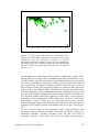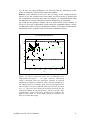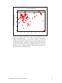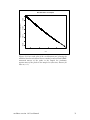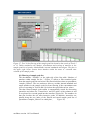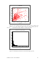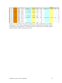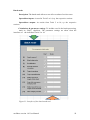
1
enviMass 1.0
target screening workflow
______________________
Martin Loos, Matthias Ruff, Heinz Singer
2011
User manual
Contact:
Martin Loos, Eawag Dübendorf, P.O. Box 611, Switzerland
Telephone
+41 (0)58 765 5118
Fax
+41 (0)58 765 5311
[email protected]
enviMass version 1.0 User Manual
1
Contents
Contents ............................................................................................................................. 2 Getting started................................................................................................................... 4 Online Installation ............................................................................................................ 7 Offline Installation ............................................................................................................ 8 Input data formats ............................................................................................................ 9 Save settings and calculation results for later usage.................................................... 10 Tool 1: Data Upload ........................................................................................................ 11 Tool 2: Data Check ......................................................................................................... 12 Tool 3: Isotopic pattern generation ............................................................................... 13 Tool 4: Match standards and target patterns............................................................... 21 Tool 5: Spark removal .................................................................................................... 23 Tool 6: Blank subtraction ............................................................................................... 26 Tool 7: Recalibration ...................................................................................................... 28 Tool 8: Internal standard screening .............................................................................. 34 Tool 9: Target screening ................................................................................................. 39 Tool 10: Target quantification ....................................................................................... 43 Tool 11: Adduct search for targets / internal standards ............................................. 45 Tool 12: Search for other non-monoisotopic peaks ..................................................... 49 Tool 13: Adduct search non-targets / non-int.stand. ................................................... 51 Tool 14: Filter sample peak list...................................................................................... 53 Batch mode ...................................................................................................................... 58 Isotopic pattern spreadsheet .......................................................................................... 59 isotopic_pattern data sheet ....................................................................................... 60 target_screening data sheet ...................................................................................... 60 targets data sheet ...................................................................................................... 60 internal standards data sheet .................................................................................... 61 sample data sheet ..................................................................................................... 62 blank data sheet ........................................................................................................ 64 adducts data sheet .................................................................................................... 64 isotopes data sheet.................................................................................................... 65 resolution.................................................................................................................. 66 known ....................................................................................................................... 66 samples_filtered ....................................................................................................... 67 non-targets................................................................................................................ 67 Limitations ....................................................................................................................... 68 Computer requirements ................................................................................................. 68 Licenses ............................................................................................................................ 68 Citing ................................................................................................................................ 69 FAQs................................................................................................................................. 70 References ........................................................................................................................ 74 enviMass version 1.0 User Manual
2
Abstract
The enviMass workflow supports screening high-resolution mass spectrometry
(HRMS) data for internal standards and target compounds and subsequent grouping of
the remaining non-target data.
Based on sample and a blank or blind HRMS peak lists, enviMass provides tools for
(a) the removal of noise data, (b) blank / blind data subtraction, (c) mass recalibration,
screening for isotopic patterns of (d) internal standards and (e) target compounds, (f)
target quantification and (g) search for additional adducts of targets / internal
standards.
Subsequent steps incorporates (h) search for non-target isotopic peak patterns and (i)
search for potential non-target adduct peaks. Finally, data are (j) summarized, filtered
and a non-target candidate list is compiled.
Tools (a) to (j) can be conveniently run in a batch mode. An additional tool allows
simulation of (profile) isotopic fine structures for molecular formulas.
The procedure is implemented in an Excel/VisualBasic setting that utilizes RExcel to
make use of the R statistical environment and its packages. Thus, speed of calculation
is strongly increased as compared to using Excel/VisualBasic alone. R and RExcel can
be downloaded and installed free of charge. All calculation steps are controlled via
user interfaces and are embedded in a convenient and selfexplaining workflow.
Parameters, workflow settings and underlying input data can be modified and
extended by the user; all data are handled in simple spreadsheet
formats.
The
enclosed isopat R package allows calculation of the isotopic fine structures
indispensable for HRMS target screening.
enviMass version 1.0 User Manual
3
Getting started
enviMass provides a full target screening framework based on convenient user
interfaces. A number of consecutive Tools 1-14 support (HR)MS data upload, data
fits to isotopic patterns of internal standard and target compounds, noise removal,
mass recalibration, screening, quantification, assemblage of candidate non-target
patterns and data filtering. The steps comprising this workflow are depicted in
Figure 1.
The workflow is implemented in the ‘target_screening’ spreadsheet of the enviMass
Excel file. The spreadsheet ‘isotopic_pattern’ computes isotopic fine structures for a
given molecular formula independently of the target screening workflow and may be
used as stand-alone tool.
Two basic input data sets are required.
(1) A list of sample peaks and, optionally, a list of blind or blank data peaks are
needed. These lists must at least contain information on (a) intensities, (b) mass-tocharge ratios (m/z) and (c) retention times for the individual peaks. These lists are
loaded into the workflow and are then stored in the spreadsheets “sample” and
“blank”.
(2) Compound lists for targets and/or internal standards are needed. These lists have
to be entered manually into the spreadsheets “targets” and “internal standards” (cp.
the Data sheets section) and contain the molecular formulas and retention times of
individual target compounds and internal standard substances.
Note: Isotopic patterns of targets and internal standards are calculated and stored in
the spreadsheets “targets” and “internal standards” for each HRMS ionization mode.
If the user wants to switch between ionization modes (i.e. between positive and
negative ionization), he has to maintain two separate enviMass worksheets. One
worksheet contains isotopic patterns calculated for positive ionization and another one
contains patterns for negative ionization.
Most tools allow to be skipped if underlying input data are missing. Thus, separate
parts of the workflow can be combined and others omitted, tailored to the needs of the
user. For example, the screening uses blind data if provided; if not provided, dummy
variables are used instead. All separate steps of the workflow are sequenced so as to
guide the user from one tool to the next in a self-explaining manner. Stepping back to
a tool further upstream from a downstream tool is disabled; the workflow
automatically manages the actions that can be conducted for the various spreadsheets
and the addition of information therein. Once all tools in the workflow have been
adjusted / parameterized to the specific needs, they can be run in a batch mode.
We recommend the user to start with the below installation section. Subsequently,
reading the section about data input formats and data upload via Tool 1 seems
apposite. Afterwards, the user may step from tool to tool reading the tool sections of
this manual. Each tool section has a tool description and gives clarification about inand outputs as well as the required / recommended parameter settings.
Alternatively, the user may continue after installation with the example workflow
which is based on the contents of the example folder found on the source website. The
example folder already includes example lists of sample and blank peaks and a
enviMass version 1.0 User Manual
4
workflow with target and internal standard compounds and exemplary parameter
settings.
Figure 1 (next page): flowchart representation of the screening workflow. Green:
input data stored in spreadsheets. Blue: input data read from text files. Yellow: output
spreadsheet lists.
enviMass version 1.0 User Manual
5
sample peak list
adduct list
data upload
blank peak list
blind peak list
isotope data
data check
isotopic pattern generation for internal standards / targets
match internal standards / targets
resolution data
batch mode
spark subtraction
blank subtraction
known deviation
recalibration
data
modification
internal standard search
internal standard screening
list of internal standards
target screening
list of targets
screening
target quantification
adduct search for targets & internal standards
adduct list
search for other (non-target / non-internal standard) isotopic pattern peaks
search for other (non-target / non-internal standard) adducts
Input
filter data
sample peak list
filtered sample peak list
list with candidate non-target peaks
enviMass version 1.0 User Manual
adduct list
preparation
of non-target
list / filtering
6
Online Installation
The screening workflow is embedded into Excel / Visual Basic (VBA) 2003, 2007 and
2010 (32 bit versions) and makes use of R code and packages via the RExcel software
under Windows XP and Windows7 32 bit OS. Therefore, RExcel and R need to be
installed on a computer via the following steps:
(1) Make sure You have Microsoft Excel 2003 or a higher version installed on
Your computer.
(2) Make sure You are online.
(3) Go to the download section of
http://rcom.univie.ac.at/
Under RExcelAndFriend download + run the online installation
RAndFriendsSetupXXXXVX.X-X-X (latest version) and let Your computer
restart; this will install the most up-to-date versions of R, RExcel,
statconnDCOM, rcom, ... on Your computer.
The mentioned webpage also provides the individual tools for offline
installation. Further information on the statconn tools, their installation and
problem handling is provided by the named website and variuos
RExcel+statconnDCOM user platforms.
Open Excel. Under Excel 2010, RExcel should appear automatically as add-in.
Otherwise, and for earlier releases of Excel, go to Start -> All Programs ->
statconn -> RExcel -> Activate RExcel as Add-In. Thereupon, open Excel (->
Add-Ins) -> RExcel -> Set R Server -> select Server type = background.
The named homepage gives detailed advices on the installation and debugging
of RExcel.
RExcel should run the workflow under the default settings. These are set under
Excel in the toolbar via RExcel -> Options (Missing values = Loose /
Dataframe name = Workbook / select DFVarnames as Rnames and Warning
before overwrite and Activate Dataframe in Rcommander and Rcommander
gets focus with output).
(4) Download the enviMass workflow from the resource webpage.
Open the enviMass_2010.xlms or enviMass_2003 & 2007.xls file to run the
target-screening workflow under Excel 2010 or Excel2007 / Excel2003,
respectively. The workflow is operated via the spreadsheet target_screening.
The user must at no point disable any Excel Visual Basic Macro functionalities,
i.e. the user must enable all spreadsheet contens.
(5) Calculation of isotopic patterns in enviMass is based on the R package
isopat. If being online while using the enviMass worksheet, this package while
be downloaded automatically at the appropriate workflow step.
enviMass version 1.0 User Manual
7
Alternatively, isopat can be downloaded manually. To do so, (a) open the R
version installed during step (3), (b) in the opened R GUI select “packages” ->
“install packages”, (c) a window with R mirrors pops up: press OK, which
opens (d) a list of packages available at this mirror site. (e) Within the list,
search for isopat, select and click OK.
Check the FAQ section for further problem handling. It also refers to startup problems
when opening the enviMass 1.0 workflow in Excel.
Offline Installation
For installing a computer without internet access, follow the steps:
For installation on PC without internet connection the individual tools R, RExcel,
Statcon have to be downloaded separately under the following links:
1. R:
http://www.r-project.org/
2. RExcel:
http://rcom.univie.ac.at/
see Download RExcel 3.2.0 in the download section
3. StatconnDCOM:
http://rcom.univie.ac.at/
see Download statconnDCOM 3.1-2B7 in the download
section
4. Isopat:
http://cran.r-project.org/
Isopat must be downloaded manually: (a) open your web
browser (internet explorer, firefox, ...) and (b) browse to
http://cran.r-project.org/. There, (c) under “CRAN” click
“search” and (d) search for “isopat”. (e) From the search
results, select “CRAN-package isopat” and the package
source site opens. This source site has a download section:
(f) there, choose the download fitting your OS, (g) unpack
the download and (h) copy + paste the unpacked folder
“isopat” into your R library folder. The R library folder
usually resides under C:\...\Program Files\R\RX.XX.X\library and contains the folders of all packages
used in your R environment.
enviMass version 1.0 User Manual
8
Input data formats
The enviMass workflow processes .txt or .dat text files with input data of (1) peak m/z,
(2) peak intensities and (3) peak retention times from HRMS measurements. Two data
sets can be loaded: firstly, a list of peaks for a measured sample must be loaded.
Secondly, a list of peaks for blank or blind measurements can be loaded. The first list
is obligatory to the enviMass workflow, the second is not.
To reduce the data size of the raw HRMS measurements, processing with a filtering
software is commonly conducted. The resulting text files of sample and blank/blind
data peak lists can be loaded via Tool 1: data upload (see below), with each line
corresponding to one peak of the HRMS scan. Filtering can be based on the Thermo
Scientific Formulator software tool, which can be downloaded from the Thermo
Electron Corporation homepage:
http://sjsupport.thermofinnigan.com/public/detail.asp?id=450
Formulator requires (1) Thermo data files (*.raw) as input and (2) Xcalibur 2.0 or
higher to be installed on your system. The enviMass data upload is adapted to the
Formulator data output format, i.e. a tab-delimited text file with 10 columns
containing numeric values only. Three of these columns contain data essential for the
workflow: column #1 (centroid m/z), column #2 (peak intensity) and column #5
(retention time). Another four columns aid at filtering noise data from the data set,
namely columns #7 and #9 (start and end retention time) and/or columns #6 and #8
(start and end scan number). However, in case that filtering is skipped (cp. Tool 5:
spark removal), these latter four columns are not essential to run the workflow.
Columns #3, #4 and #5 correspond to the peak signal to noise ratio, the scan number
and the mass chromatogram signal to noise ratio, respectively.
Alternatively, the user may work with peak data filtering tools other than Formulator,
such as MZmine:
http://mzmine.sourceforge.net/
If doing so, the user must reformat the text file to be loaded into the workflow to
adapt to the above described Formulator output format, i.e. ten columns of numeric
values (no characters; no empty line or column positions; dummy variables for
columns #3, #4 and #10 should be set to a 9999 values; not more than ten columns),
with (a) a first column of peak centroid m/z values, (b) a second one with peak
intensities, (c) a fifth one with peak retention times and - optionally - the above
columns for (d) start and end peak retention times and/or (e) start and end peak scan
numbers.
The enviMass example folder on the source website provides exemplary text files
produces from Formulator peak picking.
enviMass version 1.0 User Manual
9
Save settings and calculation results for later usage
Once the parameters in the workflow interfaces are chosen and input data sets defined
and loaded, the workflow can be saved and reused when being reopened.
Mind that the ‘Start workflow’ button of ‘Tool 1: Data upload’ DOES NOT
REMOVE the parameters typed into the textboxes of the user interface. However, it
DOES REMOVE (1) the sample and blind data sets in the spreadsheets ‘sample’ and
‘blank’ and (2) the results in the spreadsheets ‘samples_filtered’ and ‘non-targets’ and
(3) all graphs pasted into the workflow.
enviMass version 1.0 User Manual
10
Tool 1: Data Upload
Description.
Command button ‘Start workflow’ resets the workflow so that it can be started
anew (i.e. all downstream Tools are reset to operation mode). This embraces
the deletion of (1) all graphs and tables contained in the workflow and (2) the
data contained in the blank/blind input and all output spreadsheets.
Command ‘Load sample peak list’ allows upload of a text file containing peak
lists of a sample data set to be screened. Similarly, command button ‘Load
blank peak list’ allows upload of a text file with a peak list of blank or blind
data. In case no blank/blind data are available, the latter step can be skipped.
For input formats of these text files check above section ‘Input data formats’.
Spreadsheet inputs.
None.
Spreadsheet outputs.
Spreadsheets ‘sample’, ‘blank’, ‘samples_filtered’ and ‘non-targets’ are
cleared. New lists of sample data and blind / blank data are written to
spreadsheets ‘sample’ and ‘blank’.
Calculations & parameter settings.
None.
Figure 2: Data upload in the screening tool workflow.
enviMass version 1.0 User Manual
11
Tool 2: Data Check
Description.
The Tool checks the list of (a) the internal standards and (b) the targets for
consistency and missing values in columns A to O and A to Q, respectively.
Should inappropriate non-numeric values or gaps exists in these columns, an
error message is printed. If missing isotopic pattern entries are detected, the
Tool subsequently redirects the workflow to Tool 3 for calculation of the
isotopic patterns. If names or IDs in columns A and B are not unique, an error
message is printed and the errors have to be corrected before running the tool
again.
Moreover, chemical formulas in columns C are checked for consistency and
monoisotopic molecular masses are written to columns D ‘Mon. mass’ of the
target and internal standard spreadsheets.
Spreadsheet inputs.
Columns A to O and A to Q of the internal standards and target spreadsheets,
respectively.
Spreadsheet outputs.
Monoisotopic molecular masses to columns D ‘Mon. mass’ of the target and
internal standard spreadsheets.
Calculations & parameter settings.
Monoisotopic molecular mass calculation. No parameters to be set.
Figure 3: Data check tool, redirecting to Tool3 (isotopic pattern calculation).
enviMass version 1.0 User Manual
12
Tool 3: Isotopic pattern generation
Description.
The tool calculates the isotopic patterns and fine structures for the molecular
formulas of all listed (a) target compounds and (b) internal standards. It
furthermore allows for Gaussian profiling of these patterns via representation
by stick data and conversion to surviving peaks and centroid peaks.
Subsequently, these latter isotope peaks may then be filtered by Recursive
Base Peak Framing (RBPF). The isotopic peaks are stored in the spreadsheets
lists of the targets and internal standards and later used as input to the
screening Tools 8 and 9.
Spreadsheet inputs.
(1) Molecular formulas for (a) the target compounds (spreadsheet ‘targets’,
column C) and (b) the internal standards (spreadsheet ‘internal_standards’,
column D). Element names must be followed by numbers (atom counts of that
element), except for preceding numbers in square brackets indicating
individual isotopes defined in the element name column of the ‘isotope’
spreadsheet, e.g. [14]C or [18]O. For example, [13]C2C35H67N1O13 is the
molecular formula of erythromycin labeled at two C-positions with [13]C;
C37H67N1O13 is the molecular formula of the unlabeled compound.
(2) Individual adducts other than the one chosen from the workflow interface
can be defined for (a) the target compounds in spreadsheet ‘targets’, column K
and (b) the internal standards in spreadsheet ‘internal_standards’, column I
(build adduct?). To do so, instead of setting the entry for a compound to
TRUE (= using the adduct specified in the workflow interface), set it to
FALSE and include the adduct in the chemical formula directly (see above
point (1)). For example, let the compound Cytarabin have two adducts, namely
H- and Na-adducts. To include both adducts for screening, have two entries
(rows) in the target or internal standard spreadsheet list for Cytarabin. For the
H-adduct (first row), use the molecular formula of Cytarabin C9H13N3O5,
set ‘build adduct’ to TRUE and chose ‘Form adducts’ / ‘H(default)’ in the
workflow interface. For the Na-adduct however (second row), set ‘build
adduct’ to FALSE and extend the molecular formula to contain Na1, i.e.
C9H13N3O5Na1.
(3) Charges other than the one chosen from the workflow interface can be
defined for (a) the target compounds in spreadsheet ‘targets’, column L and (b)
the internal standards in spreadsheet ‘internal_standards’, column J (‘charge?’).
To do so, do not set the column entry to FALSE, but enter a value for the
charge. For example, let the compound Cytarabin have two ionization states, a
single positively charged and a double positively charged. To include both
charges for screening, have two entries (rows) in the target or internal standard
spreadsheet list for Cytarabin. For the single charge state, set the one row
entry ‘charge?’ to FALSE; here, the charge defined in the workflow interface
(set to 1) is used. In contrast, the double positively defined ionization state is
established by setting the second row entry of ‘charge?’ not to FALSE, but to
a charge value, namely 2.
(4) If resolution datasets from the spreadsheet ‘resolution’ are utilized for
defining resolving power and/or stick discretization, a preliminary check if
compound masses fall within the range of the masses of the resolution data
enviMass version 1.0 User Manual
13
sets is conducted. For this, masses for (a) targets (spreadsheet ‘targets’,
column D) and masses for (b) internal standards (spreadsheet ‘internal
standards’, column D) are utilized. These masses have been calculated by
‘Tool 2: Data Check’.
(5) If selected, resolution data sets (spreadsheet ‘resolution’) are used to define
the resolving power and/or the stick discretization width.
(6) Isotope data (spreadsheet ‘isotopes’) serves as input to the isotope pattern
calculation.
(7) Electron mass from spreadsheet ‘isotopes’.
(8) Adducts and their masses are defined in the spreadsheet ‘adducts’.
Spreadsheet outputs.
(1) Masses of isotope peaks and
(2) their abundances relative to that of the monoisotopic peak are written to
spreadsheet ‘targets’ / columns N and O and to spreadsheet
‘internal_standards’ / columns L and M for (a) the targets and (b) the internal
standards, respectively. Abundances are automatically rescaled to that of the
monoisotopic peak.
Additionally, two more dummy columns are established for each (a) the
targets (spreadsheet ‘targets’ / columns P and Q) and (b) the internal standards
(spreadsheet ‘internal_standards’ / columns N and O):
(3) The first one (‘omit peak #’) indicates which of the isotopic peaks shall be
omitted from screening when overlap between peak patterns of target
compounds and internal standards is detected (in subsequent Tool 4: Match
standards and target patterns).
(4) The second column (‘peak # for quantif.’) sets the isotopic peak used for
quantification (cp. Tool 10: Target quantification) and can be modified by the
user. As a default the intensities of the first (monoisotopic) peaks of target and
internal standard are used for quantification, i.e. these values are set to 1.
Calculations & parameter settings.
Calculations are derived in three hierarchical steps that can be selected in the
‘Output options’ of the workflow interface (Figure 4). In a first step, the
isotopic pattern is calculated. In a second optional step, a Gaussian profile is
fitted to the resulting peaks and surviving peaks extracted. In a third optional
step, Gaussian profiles are converted to centroid peak data. The peaks
resulting from the last two steps can optionally be filtered by Recursive Base
Peak Framing (RBPF).
Hence, depending on what the user selects, (a) peak data of isotopic pattern
OR (b) profile surviving peaks OR (c) profile centroid peaks are written to the
target or internal standard lists for the settings ‘Pattern’, ‘Profile’ or ‘Centroid’,
respectively; these peaks are optionally RBPF-filtered for cases (b) and (c).
General settings. For the first, mandatory step, settings have to be specified in
the ‘General Settings’ interface (Figure 5).
enviMass version 1.0 User Manual
14
Figure 4: Output options for the isotopic pattern calculation.
Figure 5: General settings for the isotopic pattern calculation.
‘Charge’ defines the ionization state of the compounds (cp. section
Spreadsheet inputs / Point (3)). For no charge, set to 0. Use a minus sign for
negative charge.
‘Abundance limit’ defines the abundance threshold below which isotopic
combinations in the molecule are not further permuted towards
othercombinations within the isotopic pattern calculation algorithm. The
defaults is set to 1E-10, but much lower values should be used for molecules
with elements having several isotopes of high abundance (cp. below section
‘Algorithm for isotopic pattern calculation’).
In contrast, ‘Abundance cutoff’ gives a threshold to filter peaks with low
abundance from the peak list after any of the steps (a) to (c), with default 1E-3.
‘Form adducts?’ specifies if adduct masses should be added to the
isotopologue masses. If selected and no adduct is chosen from the associated
list box, an hydrogen atom (‘+H(default)’) will be used as adduct.
Profile / Centroid settings. Given the above isotopic pattern, a Gaussian
profile is fitted to each peak of the pattern. The settings therefor have to be
specified in the interfaces for ‘Resolving power (FWHM)’ (Figure 6).
enviMass version 1.0 User Manual
15
Figure 6: Profile and centroid settings for the isotopic pattern calculation.
The resolving power ∆m defines the mass difference two peaks of same
intensity and with mass m1 and m2 must have to be separable by (HR)MS
(Figure 7). The resolution R is thus defined as R = ((m1+m2)/2) / ∆m (IUPAC,
1997). Three options are provided to define the resolving power ∆m: (1) as a
fixed value [mmu], (2) as function of mass [ppm] or (3) based on a selected
data sets of resolution R as function of mass provided in the spreadsheet
‘resolution’. In the latter case, a generalized additive model based on
regression splines is fitted to predict R = f(mass) (Woods, 2006). The model
then interpolates R for a given mass m and the resolving power is derived from
∆m = m / R. Given a value for the resolving power ∆m from any of the above
options (1) to (3), a standard deviation σ must be calculated for the two
Gaussian profiles of the two peaks so as to have both profiles overlap at their
Full Width at Half Maximum (FWHM) (Figure 8:). Implicitly, this specific
overlap property is henceforth assumed to make two peaks separable. For two
symmetrical distributions of two peaks of same intensity, FWHM = ∆m. The
standard deviation can then be calculated from the FWHM via the relationship
FWHM / 2√(2ln2) = σ. The parameter ‘sd factor’ allows to multiply σ with a
factor, i.e. to de- and increase the standard deviation of the profiles (default is
‘sd factor’ = 1, namely no de- or increase). Once Gaussian profiles are
calculated for each peak, they are summed so as to yield an overall profile of
the m/z spectrum (
Figure 9:).
enviMass version 1.0 User Manual
16
∆m
Figure 7: Two isotopic pattern peaks separated by resolving power ∆m.
In a next step, the resulting overall profile is converted to stick representations
(Figure 10:), with sticks having a defined distance of ∆m to each other, as
defined in the ‘Stick discretization’ section of the ‘Profile / Centroid settings’
(Figure 6). In analogy to the resolving power, ∆m can be set in three ways: (1)
as a fixed value [mmu], (2) as function of mass [ppm] or (3) as a function of
Resolution R under differing masses. Again, the latter uses the data sets from
spreadsheet ‘resolution’ and fits a spline regression model to establish R =
f(mass). At a given mass m, ∆m for stick discretization is then given by ∆m =
m / R (or, to derive ∆m in [ppm] units, ∆m [ppm] = 1E6 / R).
Often, the ∆m for stick discretization has a fixed relationship to the ∆m of the
resolving power. More precisely, to adequately depict two adjacent profiles,
the ∆m for stick discretization must be smaller than the ∆m for resolving
power. Therefore, ∆m for stick discretization may be defined as fraction of the
∆m chosen for the resolving power. The value for ‘factor’ in the ‘Stick
discretization’ settings allows for such a relationship. Given that the ∆m for
the resolving power is set with Resolution = f(mass) on a data set x, the same
data set x can be chosen for the stick discretization and a factor z specified.
Thus, the ∆m separating two sticks is z times smaller than the ∆m of the
resolving power, ensuring accurate valley stick detection between the two
peaks. Such a parameter setting is exemplified for z = 4 in Figure 6.
Next, surviving peaks or centroids are calculated for either the ‘Profile’ or the
‘Centroid’ setting, respectively. In general, two isotopic pattern peaks can be
separated if the sum of their profiles allows for a valley, which in turn is
represented by one stick encompassed by two adjacent sticks of higher
intensity (Figure 10). The surviving peaks of the ‘Profile’ setting designate
enviMass version 1.0 User Manual
17
those peaks that can be separated by a stick valley representation; for those
that cannot be separated by a valley, only the one most intensive peaks
survives. In contrast, the centroid peaks of the ‘Centroid’ setting are intensityweighted sums of those sticks that are not separated by a valley.
Finally, the isotopic pattern / surviving / centroid peaks can be optionally
filtered by Recursive Base Peak Framing (RBPF). Herein, the most intensive
peak of the data set is selected and all other peaks close enough to this peak
(within a mass tolerance = ‘frame width’ in the ‘Recursive Base Peak Framing
(RBPF) settings’) are discarded. From this reduced data set, the second most
intensive peak is selected and again other peaks in its vicinity discarded. Thus,
RBPF is recursively applied over all peaks along decreasing intensities.
Figure 8: Two isotopic peaks with profiles overlapping at FWHM.
enviMass version 1.0 User Manual
18
Figure 9: Two peaks with indiviual (green, red) and overall profiles (black).
and
Figure 10: Two peaks (red, green), the resulting overall profile (thick black)
the stick representation (black lines).
Algorithm for isotopic pattern calculation. The algorithm for deriving the
isotopic pattern for a given molecular formula is provided in the package
isopat, which has been included during installation. In contrast to other
algorithms and package implementations (cp. Rockwood et al., 2006; Kirchner,
enviMass version 1.0 User Manual
19
2008), the provided algorithm allows calculation of isotopic fine structures for
isotopologues with identical nucleon number.
Starting from a monoisotopic peak of a given molecule (e.g. C2H6, with each
elements set to those isotopes with highest abundance), the isotopic
compositions and the concomitant abundances of isotopologues are iteratively
changed towards less abundant isotopes. For a first iteration (generation i=1),
[12]C2[1]H6 would hence be changed to both [12]C1[13]C1[1]H6 and
[12]C2[1]H5[2]H1. Similarly, the latter two isotopologues then again lead to
two exhanges each for C and H at second generation i=2. At each generation
level i, a number i of isotopes contained in the monoisotopic peak have been
exchanged for less abundant isotopes over all possible permutations of size i.
Abundances are checked for <= the limit argument. If below limit, the
concerned isotopologues are not changed forward to the next generation i+1.
The methodology used for updating abundances and masses when progressing
from generation i to i+1 resembles that of Li et al. (2008). However, the
updating does not strictly follow increasing nucleon numbers. Instead,
generations of isotopic compositions are derived from an initial monoisotopic
peak (i=0) via progressing to less abundant isotopes. Furthermore, different
combination orders carried from one generation to the next can eventually lead
to the same isotopic composition at a given generation, causing double
occurrences for some peaks in a generation. Therefore, peaks are checked
against double isotopologues at each generation level. Finally, the isotopic
peak list is sorted by increasing masses. Too high values (e.g.1E-5) for the
limit may prevent the calculation of isotopologues for molecules containing
both (1) several abundant isotopes of one element (e.g.[35]Cl and [37]Cl) and
(2) many atom counts for the latter (e.g. hypothetical Cl500). On the other
hand, too low values for the limit may lead to the unnecessary calculation of
peaks with very little abundance. The user is requested to find a trade-off,
possibly by comparing peak lists derived from different limit settings using the
isotopic pattern simulation tool in spreadsheet ‘isotopic_pattern’.
enviMass version 1.0 User Manual
20
Tool 4: Match standards and target patterns
Description.
A target substance can be linked to an internal standard with known
concentration so as to quantify target concentrations via ratios of the peak
intensities of both compounds. Often, these internal standards are isotopically
labeled isotopologues of the target substance to be quantified. As a
consequence, certain peaks in the calculated isotopic patterns of both
substances may be identical, leading to an increased intensity of the resulting
net peak. If this net peak is used for quantification or screening, outcomes may
be erroneous. Therefore, Tool 4 matches the isotopic pattern peaks of the
target with those of the internal standard to which it is linked via an ID. If an
overlap between both peak patterns is detected, the concerned peaks are
marked so as to be omitted from screening and quantification.
Apart from such overlaps in peak patterns, the tool also checks the consistency
of (a) the isotopic patterns and (b) the ID-linking of a target compound to an
internal standard.
Spreadsheet inputs.
(1) Isotopic masses from column N (‘Isotopic m/z’) of the ‘target’ spreadsheet
and column L (‘Isotopic m/z’) of the ‘internal_standards’ spreadsheet.
(2) The column I (‘ID internal standard’) in the ‘targets’ spreadsheet specifies
the ID of the column A ‘ID’ in spreadsheet ‘internal_standards’ to link a target
compound to a specific internal standard for (a) quantification purposes (Tool
10) or (b) if an isotopically labeled compound of a target is listed in the
‘internal_standards’ spreadsheet making a match of isotope patterns necessary.
(3) Retention times from columns E of both spreadsheets are utilized.
Spreadsheet outputs.
(1) If an identicalness between isotopic peaks of a target compound and its
internal standard is detected, the indices of the concerned peaks are each
written to the ‘omit peak #’ columns P and N for the target and the internal
standard, respectively. For the internal standard, the string of indices is
preceded by the row number (e.g. #21:) of the target compound entry in the
spreadsheet ‘targets’ (in turn, the relation target to internal standard is
manifested by the ID value). As a consequence, the concerned peaks are
omitted at the downstream screening steps.
(2) Moreover, modifications in the column ‘peak # for quantif.’ are made to
the default value = 1 (columns Q and O for the target and the internal standard
spreadsheets, respectively).
For example, consider a target compound and an internal standard, the latter
being represented by an isotopically labeled molecule identical to that of the
target. The default peak to be used for quantification for both the target and its
internal standard is the most abundant (mostly monoisotopic) one listed in the
cells of columns N and O (targets) and columns L and M (internal standards),
i.e. peak index = 1. From labeling with heavier isotopes, the internal standard
isotopic peaks are shifted towards higher masses relative to those of the target.
Thus, there is no overlap for the target monoisotopic peak with any of those
isotopic peaks of the internal standard pattern. For the internal standard
however, the most intensive peak may indeed overlap with the target pattern.
enviMass version 1.0 User Manual
21
Hence, column O in the internal standard list does not list ‘peak # for quantif.’
= 1, but the error message “Target monoisotopic peak overlaps with
standard!”. The user is hence requested (a) to check for error messages in
these columns, (b) to set the index for the ‘peak # for quantif.’ to another value
and (c) to rerun the tool.
(3) If no peaks remain after the match (e.g. for two identical substances), (1)
an error message string is printed to the concerned cells in columns ‘omit peak
#’ and ‘peak # for quantif.’ and (2) the cell of columns ‘use for screening ?’
(column M of the target and column K of the internal standard spreadsheets) is
set to FALSE so as to omit these compounds from screening. Similarly, if (a) a
mismatch between the number of isotopic masses and isotopic abundances is
detected for a single substance or (b) several internal standards have the same
ID in column A of spreadsheet ‘internal_standards’ as referred to by column I
of the target spreadsheet, entries in column ‘use for screening ?’ are set to
FALSE and an error message is printed to columns ‘peak for quantif.’, too.
Calculations & parameter settings.
The parameter ‘∆ retention time target vs. standard [min]’ (cp.
Figure 1) states the difference in retention time between the target compound
and its ID-linked internal standard below which the isotopic pattern check
appears necessary. In other words, even if the target and its internal standard
would have a subset of identical isotopic peaks, a difference in retention time
equal or greater to the specified value would separate the peaks of both
compounds so as to have no overlap between the concerned peaks of their
isotopic patterns.
Figure 11: User interface of Tool 4.
enviMass version 1.0 User Manual
22
Tool 5: Spark removal
Description.
Peaks with a particularly short chromatographic eluation period may be
regarded as artifacts (noise, MS sparks) and consequently filtered for to reduce
the size of the peak list. Therefore, based on differences in either (1) start and
end retention times (∆ RT [min]) or (2) start and end scan number (∆ scan
number), entries in the sample peak list (spreadsheet ‘samples’) are marked as
noise data and are omitted from all downstream steps of the workflow,
including those of the screening tools.
Spreadsheet inputs.
(1) For calculation of ∆ RT, the differences in ‘End RT (min.)’ and ‘Start RT
time (min.)’ is derived from columns I and G of spreadsheet ‘sample’.
(2) For calculation of ∆ scan number, the differences in ‘End Scan Number’
and ‘Start Scan Number’ is derived from columns H and F of spreadsheet
‘sample’.
(3) For including potential target candidates in the plotting functionality,
entries in column N ‘Isotopic m/z’ and column E ‘retention time’ of the target
list (spreadsheet ‘targets’) are used.
Spreadsheet outputs.
(1) Potential sparks in the sample peak list are marked by insertion of a new
column in spreadsheet ‘sample’. This new column K with header ‘spark ?’
lists sparks as TRUE; cell entries are set to FALSE otherwise. All peaks (i.e.
rows) in the sample peak list with ‘spark ?’ = TRUE are subsequently omitted
from all workflow processes downstream of Tool 5.
Calculations & parameter settings.
The tool provides an auxiliary plotting function on the right side of the dashed
line and the spark removal settings on the left side (cp. Figure 12 and
Figure 13). (1) The plotting functionality aids at determining values ∆
RT or ∆ scan number above or below which sample peaks may be regarded as
noise data. For this purpose, command button ‘Plot histogram’ depicted in
Figure 13 plots histograms with a predefined number of histogram bars
and up to a certain value for both ∆ scan number (right plot) and ∆ RT (left
plot) for all sample peaks listed in spreadsheet ‘sample’. Consult Figure 14 for
an exemplification.
Optionally, a preliminary scan through the sample peak list for potential target
compounds is made and the ∆ scan number and ∆ RT of the resulting matches
in the sample peak list of spreadsheet ‘sample’ included in the plot (red bars).
This optional operation is enabled with the check box ‘include samples
matching targets as reference values:’. When enabled, masses of monoisotopic
peaks from target list column N are searched for in the sample peak list
column A ‘Centroid m/z’ within certain mass and retention time tolerances
specified via entries to the two text boxes below the named check box.
(2) Filtering for sparks among row entries in the sample peak list of
spreadsheet ‘sample’ is done either via values for ∆ scan number or ∆ RT
(Figure 12), i.e. unless check box ‘use scan number’ is checked, ∆ RT is used
for filtering. The list box entries allow to filter for peaks above (‘use only
enviMass version 1.0 User Manual
23
upper ...’), below (‘use only lower ...’) or above AND below (‘use both
bounds’) the values specified in the text boxes. The textboxes require entries
for ∆ RT and ∆ scan number for values below which sparks are expected
(‘remove < ... (lower bound)’) or above which sparks are expected (‘remove >
(upper bound)’).
Figure 12: Parameter interface for spark removal section of Tool 5.
enviMass version 1.0 User Manual
24
Figure 13: Histogram plots of ∆ scan number and ∆ retention time from Tool
1000
0
500
Frequency
1500
2000
5.
0.0
0.2
0.4
0.6
0.8
1.0
delta retention time (RT)
Figure 14: Histogram from the plotting functionality of the Spark removal
Tool 5 with settings ‘maximum ∆RT in histogram [min]’ = 1 and ‘number of
histogram breaks’ = 60.
The histogram suggests that a large number of entries in the sample peak list
have very low delta retention times of <0.02 minutes. These entries may be
regarded as sparks or noise data and can therefore be removed with Tool 5.
enviMass version 1.0 User Manual
25
Tool 6: Blank subtraction
Description.
Tool 6 allows to compare the list of peaks stored in spreadsheet ‘blank’ (i.e.
blank or blind data) with that of spreadsheet ‘sample’. In this way, matrix
peaks or any other background peaks (which may be
related
to
the
laboratory processing of the sample data set) can be subtracted from the
sample peak list, aiming at reducing the size of the sample peak data set. If
matches between peaks of both lists are detected, the concerned peaks (row
entries) are marked in the ‘sample’ spread-sheet. These marks subsequently
serve as input to the target and internal standard screening scores and the
filtering routine of Tool 15.
Spreadsheet inputs.
(1) Data on centroid masses from the blank peak list (spreadsheet ‘blank’,
column A ‘Centroid m/z’) and the sample peak list (spreadsheet ‘sample’,
column
A).
(2) Data on retention times from the blank peak list (spreadsheet ‘blank’,
column E ‘RT (min.)’) and the sample peak list (spreadsheet ‘sample’, column
E).
(3) Data on peak intensities from the blank peak list (spreadsheet ‘blank’,
column B ‘Intensity’) and the sample peak list (spreadsheet ‘sample’, column
B).
Spreadsheet outputs.
(1) Potential blank matches in the sample peak list are marked by insertion of
a new column in spreadsheet ‘sample’. This new column L with header
‘blank ?’ lists potential sample peaks being blanks in the sample list as TRUE;
cell entries are set to FALSE otherwise.
Calculations & parameter settings.
Figure 15 shows the user interface of the discussed blank subtraction tool.
Three tolerance settings specify the precision / accuracy with which the
matching between blank and sample peaks is conducted.
(1) A tolerance in mass (∆m/z) must be specified in the first text box; a match
between target and blank is only accepted if the difference in centroid mass
between target and internal standard is lower than this mass tolerance.
(2) Akin the tolerance in retention time (∆RT) in the second text box.
(3) Thirdly, and once the tolerances for ∆m/z and ∆RT are complied to, the
peak intensities of a potential matches between blank/blind and sample data
are compared. Namely, such a potential match is discarded if the intensities of
the blank peak is X times smaller than that of the concerned sample peak (to
be specified in text box ‘Intensity of blank times smaller than sample’). For
example, it may well be the case that a substance indeed occurs in both the
blank/blind data set and the sample data set. In the first case, this substance is
introduced to the (HR)MS analytics during laboratory processing only. In the
second case, the substance exists in the sample data already before processing
AND is additionally introduced during laboratory procedures. As a result, the
concentration (and thus the peak signal) will be higher in the second case
enviMass version 1.0 User Manual
26
relative to the first case. Thus, comparing relative intensities allows to
distinguish both cases.
Figure 15: User interface of the blank / blind subtraction Tool 6. On the right,
circles mark subtraction matches between the sample and the blind/blank data
sets in the centroid m/z vs. retention time plot.
enviMass version 1.0 User Manual
27
Tool 7: Recalibration
Description.
High Resolution Mass Spectrometers sometimes produce measurements with
m/z being systematically lower or higher than the expected m/z of the
measured substances. Often, such deviations are themselves a function of m/z
and it may be unclear whether they stem from shortcomings in either
spectrometer hardware or spectrometer software. In any case, Tool 7 allows
for a recalibration of m/z to increase the accuracy of the measurements.
The mass recalibration involves four steps. Step (a) aims at detecting the mass
deviations. For this purpose, the sample peak list is screened for internal
standard monoisotopic peaks. Having assigned potential matches between
sample and internal standard peaks, the mass differences between both are
calculated in a second step (b). Thereupon, step (c) builds a nonlinear model to
relate these mass differences Δm/z to the mass m/z of the internal standards
matched. Finally, (d) this model is utilized to correct all masses listed in the
sample peak list for the observed mass differences. The thus recalibrated
masses of the sample peak list can then optionally be utilized for all
downstream workflow tools.
Alternatively to step (a) and (b), a list of known and measured m/z values from
spreadsheet 'known' can be used for model definition of step (c).
Spreadsheet inputs.
(1) 'Centroid m/z' in column A of the 'sample' spreadsheet.
(2) Retention time 'RT (min.)' from column E of the 'sample' spreadsheet.
(3) Names of internal standard substances from column B of the 'sample'
spreadsheet.
(4) The first (monoisotopic) mass entry of the string in 'Isotopic m/z' in
column L of the spreadsheet 'internal_standards'.
(5) Column E 'retention time' from spreadsheet 'internal_standards'.
(6) Column G ‘Use for recalibration?’. If set to FALSE, the corresponding
internal standard is not included in the recalibration routine.
(7) Columns C '(m/z) measured' and column D '(m/z) expected' from
spreadsheet 'known' for a list of measured and theoretical m/z values.
Spreadsheet outputs.
The recalibration procedure adds three new columns to the peak list in the
'sample' spreadsheet:
(1) Column M 'standard?' refers to the name of the internal standard (from
column B 'internal standard name') that has been matched to this peak of the
sample peak list. If no match could be assigned, these cells are set to FALSE.
(2) Column N 'ppm deviation' shows the Δm/z between the m/z peak of the
internal standard named in Column M and the m/z peak of that sample peak in
ppm units.
(3) Column O 'recalibrated m/z' lists the recalibrated masses.
Calculations & parameter settings.
(1) The first two steps (a) and (b) of the recalibration procedure are activated
via command button 'search internal standards in sample & calculated
enviMass version 1.0 User Manual
28
deviation'. Hereby, (a) internal standards are matched to peaks in the sample
peak list and (b) deviations in mass are calculated; corresponding entries to
columns M and N of the 'sample' spreadsheet are made. The tolerances in m/z
and retention time RT between internal standard and potential match in the
sample peak list are set in the text boxes below that button (Figure 16). Since
masses are not yet recalibrated at this step, a relatively wide mass tolerance
should be used. Finally, two plots are generated to help clarifying any trend in
mass deviations (cp. Figure 17 for details). In case these first two steps of the
recalibration procedure indicate no matches (or if no internal standards are
provided in the 'internal_standards' spreadsheet), the Tool can either be
skipped or a data set from spreadsheet 'known' can be used for recalibration.
Figure 16: User interface of the recalibration tool. The upper part of the
interface aids at detecting potential internal standards in the sample peak data
set. The lower part of the tool interface uses these matches to run the mass
recalibration of the sample peak data set.
enviMass version 1.0 User Manual
29
-1
45
680
2686
320
314
675
2662
74
632
682
2685
43
2681
681
2890
54
62
696
2885
688
2887
683
78
2886
685
2888
689
2645
49
2876
2877
2684
686
2719
2692
687
39
693
315
317
2694
2678
2700
2644
2659
2796
2698 2688
692
177
318
679
2661
311
2680
690
2875
30
32
180 2863
2883
2777
76 47 2687
2865
2878 2866
2806
2696
634
323
633
2648
2643 2872
2693
2775
-2
2721
-3
mmu
2663
2869
-4
2702
100
200
300
400
500
600
700
800
m/z
Figure 17: First result plot from the recalibration tool.
Depicted are deviations in mass between theoretical values
calculated from the molecular formula of internal
standards and matches found for these internal standards in
the sample peak list (ordinate, mmu units) plotted against
the mass of these internal standards (abscissa, Da unit for
mass m; z=1).
(2) Subsequent (c) model fitting and (d) mass recalibration of peaks in the
sample peak list are triggered by command button 'Run recalibration' (Figure
16). The model relates the under point (1) determined deviations in Δm/z to the
m/z listed in spreadsheets 'sample' in columns 'ppm deviation' and 'Centroid
m/z', respectively. An additive nonlinear model is used; the user can select
from a list box if 'thin plate regression splines' or 'penalized cubic regression
splines' shall be used (Wood 2006). The difference between both spline types
is mostly negligible for the recalibration outcomes. Furthermore, the user can
also specify the number of knots used in the nonlinear model via another text
box. The knot number controls the wiggliness of the model, i.e. how easily the
model fits to local nonlinearities in the relation Δm/z versus m/z. The default
knot number is set to 10. However, we recommend the user may rerun the
'Run recalibration' button under different knot numbers to infer the requested
wiggliness of the model from the concomitant plots (see Figure 18 to Figure
20).
To use a known data set with measured versus expected masses from
spreadsheet 'known' instead of matches from steps (a) and (b) of point (1),
checkmark checkbox 'calculate deviation from the data set listed in
spreadsheet "known" ' located above the list box for spline selection (Figure
enviMass version 1.0 User Manual
30
16). In this case, mass differences are derived from the differences of the
values in columns C and D of the named spreadsheet.
Beware: If the matches do not cover the m/z range of the sample peak list
masses or too few matches have been found, an error message is printed and
the recalibration procedure must either be skipped via command button 'Skip
recalibration' or a rerun with other tolerance settings may be attempted.
(3) Aided by the graphical outputs, the user must finally decide whether to
accept or reject the recalibration results using the command buttons 'Accept
recalibration results' or 'Reject recalibration results'. If accepted, all subsequent
calculations of the workflow will be based on recalibrated masses.
non-recalibrated standards
-2
-3
-4
observed (m/z) - expected (m/z) [ppm]
-1
90% percentiles
spline fit
100
200
300
400
500
600
700
800
m/z
Figure 18: Third result plot from the recalibration tool.
Depicted are deviations
in mass between theoretical
values calculated from the molecular formula of internal
standards and matches found for these internal standards in
the sample peak list (ordinate, ppm units) plotted against the
mass of these internal standards (abscissa, Da unit for mass
m; z=1). The green line shows the model predictions for the
relation deviation as function of mass, which is used for mass
recalibration. Upper and lower dashed lines separate the
highest and lowest 5% of the data, giving an estimate of a
90% percentile data range.
enviMass version 1.0 User Manual
31
-2
-1
0
90% percentiles
-3
observed (m/z) - corrected (m/z) [ppm]
1
recalibrated standards
100
200
300
400
500
600
700
800
m/z
Figure 19: Fourth result plot from the recalibration tool.
Depicted are deviations
in mass between theoretical
values calculated from the molecular formula of internal
standards and matches found for these internal standards in the
recalibrated sample peak list (ordinate, ppm units) plotted
against the mass of the internal standards (abscissa, Da unit
for mass m; z=1). Upper and lower dashed lines separate the
highest and lowest 5% of the data.
enviMass version 1.0 User Manual
32
-0.0008
-0.0012
-0.0016
observed(m/z) - corrected (m/z)
-0.0004
Recalibration of samples
200
400
600
800
1000
m/z
Figure 20: Last result plot of the recalibration tool, plotting the
modeled absolute deviation between model-predicted and HRMSmeasured masses of the peaks in the sample list (ordinate)
against mass of the peaks in the sample list (abscissa, Da unit for
mass m; z=1).
enviMass version 1.0 User Manual
33
Tool 8: Internal standard screening
Description.
Tool 8 screens the sample peak list for matches with the isotopic patterns of
the internal standards listed in the ‘internal_standards’ spreadsheet. The
underlying routine rescales the abundance of the expected peaks in the internal
standard isotopic pattern so as to exclude peaks of too low intensity from
further consideration. Thereupon, three scores (1) to (3) are derived. A
weighted sum of all three scores leads to a final overall score for each of the
internal standards; the weights must be set by the user. Mind that score (1) is
less restrictive than score (2), and score (2) less restrictive than score (3), i.e.
score (1) ≥ score (2) ≥ score (3).
score (1) Firstly, the number of internal standard peaks expected vs. the
number of peaks found in the sample list within tolerance settings of retention
time (RT) and ∆m/z is evaluated for each internal standard compound. For
example, if 6 peaks are expected but only 4 found in the sample peak list,
score 1 would result in 4 of 6 peaks, i.e. score 1 = 4/6 = 0.67 .
score (2) Based on the peaks found, the agreement of expected (= rescaled
abundance) versus observed peak intensities is evaluated for a second score.
For example, from the above 4 peaks, only 3 peaks are within the expected
intensity range (the range being set by an intensity tolerance of +/- x % of the
expected intensity). Thus, score 2 = 3/6 = 0.50 .
score (3) is even more restrictive: it also checks for interference of the
remaining peaks with those of the blank/blind peak list of spreadsheet ‘blank’.
For example, of the above 3 peaks found in the sample peak list, one peak
already has been matched in Tool 6 with a peak of the blind/blank peak list, i.e.
2 of 6 peaks remain. Therefore, score 3 = 2/6 = 0.33 .
Occasionally, different sets of peaks from the sample peak list can be matched
to one internal standard isotopic pattern set of peaks. In this case, scores for all
sets are calculated and only the results for the sets with the two best scores are
printed.
The tool provides a detailed list of achieved accuracies in (a) ∆m/z, (b) RT and
(c) intensity for the peaks matched for score 1. The tool furthermore stores
which sample list peaks are matched to which internal standards peak.
Spreadsheet inputs.
The screening tool compares peak information from the ‘internal standards’
list with peak information from the sample peak list.
The following columns from spreadsheet ‘internal_standards’ are used:
(1) Column L (‘Isotopic m/z’) and column M (‘Isotopic abundance’) provide
isotopic peak masses and abundances. They are a result of Tool 3.
(2) Column A (‘ID’) for the internal standard ID.
(3) ‘retention time’ from spreadsheet ‘internal_standards’, column E.
(4) Column K (‘use for screening?’) allows to omit internal standard entries
(rows) in spreadsheet ‘internal_standards’ from being used in the screening.
(5) Column N (‘omit peak #’) states the index of which peaks of the isotopic
pattern of a single internal standard should be omitted from screening (cp.
Tool 4).
The following columns from spreadsheet ‘sample’ are used:
enviMass version 1.0 User Manual
34
(6) ‘Centroid m/z’ in column A.
(7) ‘recalibrated m/z’ in column O of the ‘sample’ spreadsheet instead of (5) if
recalibrated sample peak list masses are used for screening (cp. Tool 7).
(8) Retention time ‘RT (min.)’.
(9) ‘Intensity’ from column A.
(10) ‘blank?’ from column L.
Spreadsheet outputs.
The screening routine makes entries to both the ‘sample’ and the
‘internal_standards’ spreadsheets.
Entries to the ‘internal_standards’ spreadsheet are exemplified in Figure 22.
Occasionally, different sets of peaks from the sample peak list can be matched
to one internal standard isotopic pattern set of peaks if several sample peaks
match to the most abundant peak (denoted as “monoisotopic hit”) of the
internal standard isotopic pattern. In this case, scores for all possible sets are
calculated and only the results for the sets with the best two scores 1 are
printed. Thus, the first block of results in spreadsheet ‘internal_standards’ (i.e.
nine columns Q to Y) refers to the set of sample peaks with the best score 1
for a match with an internal standard isotopic pattern. The second block in the
nine columns Z to AH refers to results from the set with the second best score
1. Overall, 1 + 2 x 9 = 19 new columns are assigned to spreadsheet
‘internal_standards’:
(1) Column P (‘Monoisotopic hits’) lists the ID number(s) (from column R /
‘sample ID for standard screening’ / ‘sample’ spreadsheet) of sample peak(s)
to which the most abundant peak (mostly the monoisotopic one) of the internal
standard isotopic pattern could be matched to. If no matches were found, the
entry value is set 0.
(2) Columns Q and Z (‘Isotopic hits #’) list the ID number(s) (from column R
/ ‘sample ID for standard screening’ / ‘sample’ spreadsheet) of all those
sample peak(s) to which the rescaled internal standard isotopic pattern could
be matched to. In other words, not only the most abundant peak as in point (1)
is listed here, but all those sample peaks referred to by score 1. That is, if score
1 states e.g. 4 of 6 (6 = count of expected internals standard peaks after
rescaling), four peaks are listed. The first ID number in the string (i.e. the most
abundant one) is identical to the one(s) listed under point (1).
(3) Columns R and AA (‘delta m/z (ppm)’) list the accuracy in ∆m/z between
matched sample peaks (cp. column A,’sample’ spreadsheet) and expected
peaks (cp. column L, ‘internal_standards’ spreadsheet) (i.e. ∆m/z = measured
- expected) for all those peaks listed under point (2).
(4) Columns S and AB (‘delta RT’) list the accuracy in RT between matched
sample peaks (cp. column E, ’sample’ spreadsheet) and expected peaks (cp.
column E, ‘internal_standards’ spreadsheet) (i.e. ∆RT = measured - expected)
for each of those peaks listed under point (2).
(5) Columns T and AC (‘delta intens’) list the accuracy in intensity between
matched sample peaks (cp. column B, ’sample’ spreadsheet) and expected
peaks (after rescaling of column M, ‘internal_standards’ spreadsheet) (i.e.
difference in intensity = observed - expected) for each of those peaks listed
under point (2).
enviMass version 1.0 User Manual
35
(6) Columns U and AD (‘score 1’) show score 1 for each internal standard.
(7) Columns V and AE (‘score 2’) show score 2 for each internal standard.
(8) Columns W and AF (‘score 3’) show score 3 for each internal standard.
(9) Columns X and AG (‘sum score’) gives the weighted sum of scores 1 to 3
from columns U to W and AD to AF, respectively.
(10) Columns Y and AH (‘conc [ng./l]’) are established but remain empty.
Cells will be filled with estimates of concentrations [ng/l] by using the
quantification Tool 10 after screening for internal standards and targets.
Three entries are made to spreadsheet ‘sample’:
(11) Columns P (‘monoisotopic hit for standard #’) of spreadsheet ‘sample’
lists the ID of the internal standard (column A) for which a monoisotopic hit
was matched to this peak of the sample peak list.
(12) Column Q (‘isotopic hit for standard #’) of spreadsheet ‘sample’ lists the
ID of the internal standard (column A) for which a hit of any of its peaks from
its isotopic pattern was matched to this peak of the sample peak list.
(13) Column R (‘sample ID for standard screening’) of spreadsheet ‘sample’
gives an ID to each row (peak) of the sample peak list. This unique ID is used
to identify sample peaks from entries in the screening results written to the
‘internal_standards’ spreadsheet.
Calculations & parameter settings.
The below steps are passed for each internal standard listed in the
‘internal_standards’ spreadsheet:
(1) In a very first step, a match between (a) the most abundant peak of each
internal standard isotopic pattern (first entry in the strings of columns L and M
/ spreadsheet ‘internal_standards’) and (b) a peak of the sample peak list is
screened for within tolerance settings of ∆m/z and ∆RT. Parameters for these
tolerances have to be specified in the textboxes ‘∆m/z’ and ‘∆RT listed vs.
measured [min]’, respectively. If recalibration results were accepted in Tool 7,
recalibrated masses from column O instead of non-recalibrated ones from
column A of the ‘sample’ spreadsheet are used.
Occasionally, this first step can lead to several hits in the sample peak list,
depending on the tolerance settings. In this case, below steps (2) to (6) are
passed for each of these hits, leading to several result sets. The routine outputs
only the two best ones to the ‘internal_standards’ spreadsheet, based on score
1.
(2) Thereupon, internal standard peaks with too low abundances are identified.
Provided that the above named single peak hits (a) vs. (b) were found, the
abundances taken from column M / spreadsheet ‘internal_standards’ are
rescaled to the intensity of the sample peak (b). Isotopic pattern peaks of the
internal standard with a rescaled abundance (i.e. an expected intensity) lower
than the value specified in text box ‘Intensity cutoff (default=5000)’ are then
omitted from further considerations. This step avoids to falsely screen for
expected internal standard peaks which cannot surmount the detection / noise
thresholds intrinsic to the sample peak list data set.
For example, consider (a) an internal standard isotopic pattern with
abundances = [1,0.5,0.25,0.1] and (b) a matched sample peak with intensity
(column B / spreadsheet ‘sample’) = 50000. Rescaling the internal standard
enviMass version 1.0 User Manual
36
abundances to the sample peak intensity leads to the expected intensities =
[50000,25000,12500,5000]. Thus, for an exemplary intensity cutoff = 15000,
only the first two internal standard peaks with expected intensities =
[50000,25000,-,-] would be screened for.
(3) The rescaled (i.e. reduced) isotopic pattern peak set of an internal standard
is screened for in a third step. While the tolerance parameter for ∆m/z is still
taken from the textbox ‘∆m/z’, a different tolerance parameter for ∆RT then
the one of point (1) is now used, namely the one from text box ‘∆ RT within
scan [min]’. The former tolerance in RT determined the search for the most
abundant peak of an internal standard under point (1), based on the RT listed
for each internal standard (column E, spreadsheet ‘internal_standards’).
However, a second (preferably narrower) RT is now used for screening the
other peaks of the rescaled isotopic pattern set of peaks (specified in text box
‘∆ RT within scan [min]’). The reason being, if a peak of the sample peak list
indeed represents a monoisotopic peak of an internal standard, all other sample
peaks representing the rescaled internal standard isotopic pattern should elute
at the very same retention time.
(4) Given the matched set of sample peaks, the above scores (1) to (3) are
calculated. The parameter for tolerance in intensity has to be specified in text
box ‘% Intensity’.
(5) An overall score is calculated as weighted sum of the sores (1) to (3). The
weights have to be assigned by the user through the three lowermost textboxes
of Figure 21.
(6) Accuracies in ∆m/z, ∆RT and intensity are calculated and plotted. They
may help to identify outliers from screening of the internal standard list.
(7) Note: two cases exist for which NOT the monoisotopic peak is used in step
(1). Firstly, the routine omits internal standard peaks overlapping with those
of targets (cp. Tool 4). In that case, the most abundant internal standard peak
not omitted is utilized for point (1). Similarly, all other peaks of the internal
standard not omitted are used in points (2) to (5). Secondly, rare cases exist
under which not the monoisotopic peak but another isotopologue has highest
abundance for an internal standard (e.g. C6Cl6 with maximum abundance
rescaled to monoisotopic peak = 1.9). In these cases, the most abundant peak
used for point (1) is simply not the monoisotopic one.
enviMass version 1.0 User Manual
37
Figure 21: Interface of the screening tool for internal standards in the sample peak
list.
Figure 22: Subtable in the ‘internal_standards’ spreadsheet, listing the results for the
screening of internal standards (Tool 8) on the first monoisotopic match found in the
sample peak data set.
enviMass version 1.0 User Manual
38
Tool 9: Target screening
Description.
In close to analogy to Tool 8, Tool 9 screens the sample peak list for matches
with the target compounds listed in the ‘targets’ spreadsheet. The underlying
routine rescales the abundance of the expected peaks in the target isotopic
pattern so as to exclude peaks of too low intensity from further consideration.
Thereupon, three scores (1) to (3) are derived. A weighted sum of all three
scores leads to a final overall score for each of the target compounds; the
weights must be set by the user. Mind that score (1) is less restrictive than
score (2), and score (2) less restrictive than score (3), i.e. score (1) ≥ score (2)
≥ score (3).
score (1) Firstly, the number of target compound peaks expected vs. the
number of peaks found in the sample list within tolerance settings of retention
time (RT) and ∆m/z is evaluated for each target compound. For example, if 6
peaks are expected but only 4 found in the sample peak list, score 1 would
result in 4 of 6 peaks, i.e. score 1 = 4/6 = 0.67 .
score (2) Based on the peaks found, the agreement of expected (= rescaled
abundance) versus observed peak intensities is evaluated for a second score.
For example, from the above 4 peaks, only 3 peaks are within the expected
intensity range (the range being set by an intensity tolerance of +/- x % of the
expected intensity). Thus, score 2 = 3/6 = 0.50 .
score (3) is even more restrictive: it also checks for interference of the
remaining peaks with those of the blank/blind peak list of spreadsheet ‘blank’.
For example, of the above 3 peaks found in the sample peak list, one peak
already has been matched in Tool 6 with a peak of the blind/blank peak list, i.e.
2 of 6 peaks remain. Therefore, score 3 = 2/6 = 0.33 .
Occasionally, different sets of peaks from the sample peak list can be matched
to one target isotopic pattern set of peaks. In this case, scores for all sets are
calculated and only the results for the sets with the two best scores are printed.
The tool provides a detailed list of achieved accuracies in (a) ∆m/z, (b) RT and
(c) intensity for the peaks matched for score 1. The tool furthermore stores
which sample list peaks are matched to which target substance peak.
Spreadsheet inputs.
The screening tool compares peak information from the ‘internal standards’
list with peak information from the sample peak list.
The following columns from spreadsheet ‘targets’ are used:
(1) Column N (‘Isotopic m/z’) and column O (‘Isotopic abundance’) of
spreadsheet ‘targets’ provide isotopic peak masses and abundances. They are a
result of Tool 3.
(2) Column A (‘ID’) for the internal standard ID.
(3) ‘retention time’ from spreadsheet ‘targets’, column E.
(4) Column M (‘use for screening?’) allows to omit target compound entries
(rows) in spreadsheet ‘targets’ from being used in the screening.
(5) Column P (‘omit peak #’) states the index of which peaks of the isotopic
pattern of a single target substance should be omitted from screening (cp. Tool
4).
The following columns from spreadsheet ‘sample’ are used:
enviMass version 1.0 User Manual
39
(6) ‘Centroid m/z’ in column A of the ‘sample’ spreadsheet.
(7) ‘recalibrated m/z’ in column O of the ‘sample’ spreadsheet instead of (5) if
recalibrated sample peak list masses are used for screening (cp. Tool 7).
(8) Retention time ‘RT (min.)’ from column E of the ‘sample’ spreadsheet.
(9) ‘Intensity’ from column A of the ‘sample’ spreadsheet.
(10) ‘blank?’ from column L of the ‘sample’ spreadsheet.
Spreadsheet outputs.
The screening routine makes entries to both the ‘sample’ and the ‘targets’
spreadsheets.
Entries to the ‘targets’ spreadsheet are comparable to those generated in Tool
8 and depicted in Figure 22. Occasionally, different sets of peaks from the
sample peak list can be matched to one target compound isotopic pattern set of
peaks if several sample peaks match to the most abundant peak (denoted as
“monoisotopic hit”) of that target isotopic pattern. In this case, scores for all
possible sets are calculated and only the results for the sets with the best two
scores 1 are printed. Thus, the first block of results in spreadsheet ‘targets’ (i.e.
nine columns S to AA) refers to the set of sample peaks with the best score 1
for a match with a target compound isotopic pattern. The second block in the
nine columns AB to AJ refers to results from the set with the second best score
1. Overall, 1 + 2 x 9 = 19 new columns are assigned to spreadsheet ‘targets’:
(1) Column R (‘Monoisotopic hits’) lists the ID number(s) (from column R /
‘sample ID for standard screening’ / ‘sample’ spreadsheet) of sample peak(s)
to which the most abundant peak (mostly the monoisotopic one) of the target
compound isotopic pattern could be matched to. If no matches were found, the
entry value is set 0.
(2) Columns S and AB (‘Isotopic hits #’) list the ID number(s) (from column
R / ‘sample ID for standard screening’ / ‘sample’ spreadsheet) of all those
sample peak(s) to which the rescaled target compound isotopic pattern could
be matched to. In other words, not only the most abundant peak as in point (1)
is listed here, but all those sample peaks referred to by score 1. That is, if score
1 states e.g. 4 of 6 (6 = count of expected internals standard peaks after
rescaling), four peaks are listed. The first ID number in the string (i.e. the most
abundant one) is identical to the one(s) listed under point (1).
(3) Columns T and AC (‘delta m/z (ppm)’) list the accuracy in ∆m/z between
matched sample peaks (cp. column A,’sample’ spreadsheet) (i.e. ∆m/z =
measured - expected) and for all those peaks listed under point (2).
(4) Columns U and AD (‘delta RT’) list the accuracy in RT between matched
sample peaks (cp. column E, ’sample’ spreadsheet) and expected peaks (cp.
column E, ‘targets’ spreadsheet) (i.e. RT = measured - expected) for each of
those peaks listed under point (2).
(5) Columns V and AE (‘delta intens’) list the accuracy in intensity between
matched sample peaks (cp. column B, ’sample’ spreadsheet) and expected
peaks (after rescaling of column O, ‘targets’ spreadsheet) (i.e. intensity
differences = measured - expected) for each of those peaks listed under point
(2).
(6) Columns W and AF (‘score 1’) show score 1 for each internal standard.
(7) Columns X and AG (‘score 2’) show score 2 for each internal standard.
enviMass version 1.0 User Manual
40
(8) Columns Y and AH (‘score 3’) show score 3 for each internal standard.
(9) Columns Z and AI (‘sum score’) gives the weighted sum of scores 1 to 3
from columns W to Y and AF to AH, respectively.
(10) Columns AA and AJ (‘conc [ng./l]’) are established but remain empty.
Cells will be filled with estimates of concentrations [ng/l] by using the
quantification Tool 10 after screening for both the internal standards and the
target compounds.
Three entries are made to spreadsheet ‘sample’:
(11) Columns S (‘monoisotopic hit for target #’) of spreadsheet ‘sample’ lists
the ID of the target substance (column A) from spreadsheet ‘targets’ for which
a monoisotopic hit was matched to this peak of the sample peak list.
(12) Column T (‘isotopic hit for target #’) of spreadsheet ‘sample’ lists the ID
of the target substance (column A) from spreadsheet ‘targets’ for which a hit
of any of its expected peaks from its isotopic pattern was matched to this peak
of the sample peak list.
(13) Column U (‘sample ID for target screening’) of spreadsheet ‘sample’
gives an ID to each row (peak) of the sample peak list. This unique ID is used
to identify sample peaks from entries in the screening results written to the
‘targets’ spreadsheet.
Calculations & parameter settings.
The below steps are passed for each target compound listed in the ‘targets’
spreadsheet:
(1) In a very first step, a match between (a) the most abundant peak of each
target compound isotopic pattern (first entry in the strings of columns L and M
/ spreadsheet ‘targets) and (b) a peak of the sample peak list is screened for
within tolerance settings of ∆m/z and ∆RT. Parameters for these tolerances
have to be specified in the textboxes ‘∆m/z’ and ‘∆RT listed vs. measured
[min]’, respectively. If recalibration results were accepted in Tool 7,
recalibrated masses from column O instead of non-recalibrated ones from
column A of the ‘sample’ spreadsheet are used.
Occasionally, this first step can lead to several hits in the sample peak list,
depending on the tolerance settings. In this case, below steps (2) to (6) are
passed for each of these hits, leading to several result sets. The routine outputs
only the two best ones to the ‘targets spreadsheet, based on score 1.
(2) Thereupon, target compound peaks with too low abundances are identified.
Provided that the above named single peak hits (a) vs. (b) were found, the
abundances taken from column M / spreadsheet ‘targets are rescaled to the
intensity of the sample peak (b). Isotopic pattern peaks of the target compound
with a rescaled abundance (i.e. an expected intensity) lower than the value
specified in text box ‘Intensity cutoff (default=5000)’ are then omitted from
further considerations. This step avoids to falsely screen for expected target
compound peaks which cannot surmount the detection / noise thresholds
intrinsic to the sample peak list data set.
For example, consider (a) a target compound isotopic pattern with abundances
= [1,0.5,0.25,0.1] and (b) a matched sample peak with intensity (column B /
spreadsheet ‘sample’) = 50000. Rescaling the target compound abundances to
the sample peak intensity leads to the expected intensities =
enviMass version 1.0 User Manual
41
[50000,25000,12500,5000]. Thus, for an exemplary intensity cutoff = 15000,
only the first two target compound peaks with expected intensities =
[50000,25000,-,-] would be screened for.
(3) The rescaled (i.e. reduced) isotopic pattern peak set of a target compound
is screened for in a third step. While the tolerance parameter for ∆m/z is still
taken from the textbox ‘∆m/z’, a different tolerance parameter for ∆RT then
the one of point (1) is now used, namely the one from text box ‘∆ RT within
scan [min]’. The former tolerance in RT determined the search for the most
abundant peak of a target compound under point (1), based on the RT listed
for each target compound (column E, spreadsheet ‘targets). However, a second
(preferably narrower) RT is now used for screening the other peaks of the
rescaled isotopic pattern set of peaks (specified in text box ‘∆ RT within scan
[min]’). The reason being, if a peak of the sample peak list indeed represents a
monoisotopic peak of a target compound, all other sample peaks representing
the rescaled target compound isotopic pattern should eluate at the very same
retention time.
(4) Given the matched set of sample peaks, the above scores (1) to (3) are
calculated. The parameter for tolerance in intensity has to be specified in text
box ‘% Intensity’.
(5) An overall score is calculated as weighted sum of the sores (1) to (3). The
weights have to be assigned by the user through the three lowermost textboxes
of Figure 21.
(6) Accuracies in ∆m/z, ∆RT and intensity are calculated and plotted. They
may help to identify outliers from screening of the target compound list.
(7) Note: two cases exist for which NOT the monoisotopic peak is used in step
(1). Firstly, the routine omits target compound peaks overlapping with those
of targets (cp. Tool 4). In that case, the most abundant target compound peak
not omitted is utilized for point (1). Similarly, all other peaks of the target
compound not omitted are used in points (2) to (5). Secondly, rare cases exist
under which not the monoisotopic peak but another isotopologue has highest
abundance for a target compound (e.g. C6Cl6 with maximum abundance
rescaled to monoisotopic peak = 1.9). In these cases, the most abundant peak
used for point (1) is simply not the monoisotopic one.
enviMass version 1.0 User Manual
42
Tool 10: Target quantification
Description.
Tool 10 allows for quantification of target compounds. For this purpose, any
target compound [a] to be quantified is linked via an ID to a specific internal
standard [b]. Based on results of the screening Tools 8 and 9,
- the intensity I([a]) of the sample peak to which a match with the most
abundant peak of the isotopic pattern of target compound [a] is
found and
- the intensity I([b]) of the sample peak to which a match with the most
abundant peak of the isotopic pattern of internal standard [b]
isotopic is
assigned
are set in relation Q = I([a])/I([b]) . From values of slope s and intercept q
(often q = 0) from spreadsheet ‘targets’, the ratio C of concentrations c([a]) /
c([b]) [ng/l] of target vs. internal standard are then approximated via the
simple linear relation
Q=q+s*C
Spreadsheet inputs.
- From the ‘targets’ spreadsheet:
(1) Column G ‘intercept’ gives values of q for each target compound.
(2) Column H ‘slope’ gives values of s for each target compound.
(3) Column I ‘ID internal standard’ links each target [a] to the internal
standard [b] used for its quantification. The ID values of this column I refer to
those IDs listed in column A of the ‘internal_standards’ spreadsheet.
(4) Column Q ‘peak # for quantif.’ gives the index of the expected isotopic
pattern peak of columns N and O to be used for quantification. The intensity
of the sample peak matched to this single expected isotopic pattern peak is
then used as I([a]) :
(5) The under point (4) indexed entry in each string of columns S and AB
‘Isotopic hits #’ give the IDs of the matched sample peaks. In turn, these IDs
of the matched sample peaks are entries in column U (‘sample ID for target
screening’) of spreadsheet ‘sample’.
- From the ‘internal_standards’ spreadsheet:
(6) Column A of the ‘internal_standards’ spreadsheet for internal standard IDs.
(7) Column O ‘peak # for quantif.’ gives the index of the expected isotopic
pattern peak of columns L and OM to be used for quantification. The intensity
of the sample peak matched to this single expected isotopic pattern peak is
then used as I([b]) :
(8) The under point (7) indexed entry in the string of columns Q ‘Isotopic hits
#’ gives the ID of the matched sample peak. In turn, this ID of the matched
sample peak is an entry in column R (‘sample ID for standard screening’) of
spreadsheet ‘sample’.
- From the ‘sample’ spreadsheet:
(9) IDs from column U (‘sample ID for target screening’).
enviMass version 1.0 User Manual
43
(10) IDs from column R (‘sample ID for standard screening’).
(11) Values from column B ‘Intensity’ referenced with IDs from column U
(‘sample ID for target screening’) and column R (‘sample ID for standard
screening’) serve as I([a]) and I([b]), respectively.
Spreadsheet outputs.
Two entries are made to spreadsheet ‘targets’
(1) Concentration ratio C is written to column AA ‘conc. ratio’. It is calculated
with the sample peak intensity I([a]) referenced to via an entry in the ID string
of column S ‘Isotopic hits #’. The entry of this string is in turn indexed via
information from column Q ‘peak # for quantif.’.
(2) Concentration ratio C is written to column AJ ’conc. ratio’. It is calculated
with the sample peak intensity I([a]) referenced to via an entry in the ID string
of column AB ‘Isotopic hits #’. The entry of this string is in turn indexed via
information from column Q ‘peak # for quantif.’.
Figure 23: Target quantification Tool 10.
Calculations & parameter settings.
No parameters have to specified via text boxes; the tool solely uses results
from the preceding screening Tools 8 and 9 and information stored in the
spreadsheets ‘targets’, ‘internal_standards’ and ‘sample’.
Note: If columns Q or O (‘peak # for quantif.’) of spreadsheet ‘targets’ or
spreadsheet ‘internal_standards’ index outside of the number of ‘Isotopic hits
#’ contained in columns S / AB (spreadsheet ‘targets’) and column Q
(spreadsheet ‘internal_standards’), no quantification is possible and an error
message is printed to columns S / AB (spreadsheet ‘targets’) or column Q
(spreadsheet ‘internal_standards’). For example, let ‘peak # for quantif.’ be set
to 3. If an ‘Isotopic hits #’ ID string such as ‘# 2036 / 2040’ only refers to two
peaks of the sample peak list, no third peak would be available for
quantification.
enviMass version 1.0 User Manual
44
Tool 11: Adduct search for targets / internal standards
Description.
The internal standard and target adducts which are screened for in Tools 8 and
9 are appointed in Tool 3 during the isotopic pattern generation. For example,
let Tool 3 use the adduct ‘+H(default)’ (hydrogen) to calculate the isotopic
patterns of the target compounds and internal standards. As a consequence, the
screening Tools 8 and 9 using these isotopic patterns screen for hydrogen
adducts. However, other potential adducts than the one appointed in Tool 3
may be expected. Based on the Tool 8 and 9 screening results, Tool 11 allows
to search for such potential adducts in the sample peak list.
Note: This tool screens for adducts other than the one(s) defined via Tool 3 for
isotopic pattern generation, over ALL targets and internal standards listed in
the spreadsheets ‘targets’ and ‘internal_standards’ having a sufficiently high
screening sum score. If you only want to screen for adducts
for
PARTICULAR targets and internal standards, include them directly in the
spreadsheets ‘targets’ and ‘internal standards’ prior to using Tool 3 (see point
(2) under ‘spreadsheet inputs’ in section ‘Tool 3: Isotopic pattern generation’).
Spreadsheet inputs.
From spreadsheet ‘sample’:
(1) Column A, ‘Centroid m/z’
(2) Column E, ‘RT (min)’
(3) Column U, ‘sample ID’
From spreadsheet ‘internal standards’:
(4) Column A for IDs of internal standards
(5) Column K, ‘use for screening’. Internal standards not used for screening
(FALSE) are ab initio excluded from the calculations of Tool 11.
(6) Column Q, ‘Isotopic hits #’. Lists sample peak IDs of column U in
spreadsheet ‘sample’.
7) Column X, ‘sum score’. Lists the screening Tool 9 sum score for the best
monoisotopic hit.
(8) Column Z, ‘Isotopic hits #’. Lists sample peak IDs of column U in
spreadsheet ‘sample’.
(9) Column AG, ‘sum score’. Lists the screening Tool 9 sum score for the
second best monoisotopic hit.
From spreadsheet ‘targets’:
(10) Column A for IDs of internal standards
(11) Column M, ‘use for screening’. Target compounds not used for screening
(FALSE) are ab initio excluded from the calculations of Tool 11.
(12) Column S, ‘Isotopic hits #’. Lists sample peak IDs of column U in
spreadsheet ‘sample’.
(13) Column Z, ‘sum score’. Lists the screening Tool 9 sum score for the best
monoisotopic hit.
(14) Column AB, ‘Isotopic hits #’. Lists sample peak IDs of column U in
spreadsheet ‘sample’.
(15) Column AI, ‘sum score’. Lists the screening Tool 9 sum score for the
second best monoisotopic hit.
From spreadsheet ‘adducts’:
(16) Column B, ‘Adduct name’.
enviMass version 1.0 User Manual
45
(17) Column C, ‘Adduct mass’.
Spreadsheet outputs.
Four entries are made to spreadsheet ‘sample’:
(1) Column V ‘Target adducts monoisot. #1’ lists the adduct name and the ID
(column A / spreadsheet ‘targets’) of that target compound to which the
sample peak was matched as a potential adduct. More precisely, the sample
peak was matched to one of the entries in the string contained in the target cell
of column S / spreadsheet ‘targets’ (i.e. generated in Tool 9 after matching to
the first monoisotopic target peak).
(2) Column W ‘Target adducts monoisot. #2’ lists the adduct name and the ID
of (column A / spreadsheet ‘targets’) of that target compound to which the
sample peak was matched as a potential adduct. More precisely, the sample
peak was matched to one of the entries in the string contained in the target cell
of column AB / spreadsheet ‘targets’ (i.e. generated in Tool 9 after matching
to the second monoisotopic target peak).
(3) Column X ‘Standard adducts monoisot. #1’ lists the adduct name and the
ID (column A / spreadsheet ‘internal_standards’) of that internal standard
compound to which the sample peak was matched as a potential adduct. More
precisely, the sample peak was matched to one of the entries in the string
contained in the internal standard cell of column Q / spreadsheet
‘internal_standards’ (i.e. generated in Tool 10 after matching to the first
monoisotopic target peak).
(4) Column Y ‘Standard adducts monoisot. #2’ lists the adduct name and the
ID (column A / spreadsheet ‘internal_standards’) of that internal standard
compound to which the sample peak was matched as a potential adduct. More
precisely, the sample peak was matched to one of the entries in the string
contained in the internal standard cell of column Z / spreadsheet
‘internal_standards’ (i.e. generated in Tool 10 after matching to the second
monoisotopic target peak).
Two entries are made to spreadsheet ‘internal_standards’:
(5) Column AI ‘adducts for first monoisotopic hit pattern’ lists, per internal
standard, the adduct name and the sample peak ID (contained in column U in
spreadsheet ‘sample’) of the concomitant matched peak in the sample peak list.
Here, matching refers to adducts found for the screening results of column Q
(‘isotopic hits #’) / ‘internal_standards’ spreadsheet.
(6) Column AJ ‘adducts for second monoisotopic hit pattern’ lists, per internal
standard, the adduct name and the sample peak ID (contained in column U in
spreadsheet ‘sample’) of the concomitant matched peak in the sample peak list.
Here, matching refers to adducts found for the screening results of column Z
(‘isotopic hits #’) / ‘internal_standards’ spreadsheet.
Two entries are made to spreadsheet ‘targets’:
(7) Column AK ‘adducts for first monoisotopic hit pattern’ lists, per target
compound, the adduct name and the sample peak ID (contained in column U
in spreadsheet ‘sample’) of the concomitant matched peak in the sample peak
list. Here, matching refers to adducts found for the screening results of column
S (‘isotopic hits #’) / ‘targets’ spreadsheet.
(8) Column AL ‘adducts for second monoisotopic hit pattern’ lists, per target
compound, the adduct name and the sample peak ID (contained in column U
in spreadsheet ‘sample’) of the concomitant matched peak in the sample peak
enviMass version 1.0 User Manual
46
list. Here, matching refers to adducts found for the screening results of column
AB (‘isotopic hits #’) / ‘targets’ spreadsheet.
Figure 24: Tool 11: Adduct search for target compounds and internals
standards.
Calculations & parameter settings.
Screening Tools 8 and 9 have listed results for matching isotopic patterns of
internal standards and targets with peaks (rows) of the sample peak list. The
results can be found in columns S and AB of the ‘target’ spreadsheet and in
columns Q and Z of the ‘internal_standards’ spreadsheet; they contain the IDs
of the sample peaks matched. Adduct search is now conducted via these
sample peaks matched. For example, the routine uses the ID string ‘# 3849 /
3818 / 3787’ (target column S) to extract three peaks from the ‘sample’
spreadsheet via the therein listed ID of column U (‘sample ID’) - provided the
sum score in column Z is higher or equal to the value specified in Tool 11 text
box ‘score threshold’. The routine then (a) subtracts the adduct mass used for
calculating the target isotopic pattern from each of these sample peaks and (b)
enviMass version 1.0 User Manual
47
adds masses for the adducts searched for in Tool 11. The resulting masses are
then used for screening the sample peak list for additional adduct peaks.
The adducts to be used in Tool 11 have to be selected from the interface list
box, cp. Figure 24. Furthermore, the adduct screening requires tolerance
settings from two interface text boxes for ‘∆m/z’ and ‘∆ RT within scan [min]’.
Text box ‘score threshold’ allows to exclude targets and internal standards
from the adduct search, if their screening sum score (columns AI or Z of
spreadsheet ‘targets’ / columns X or AG of spreadsheet ‘internal_standards’)
is below the value defined in that text box.
enviMass version 1.0 User Manual
48
Tool 12: Search for other non-monoisotopic peaks
Description.
Tool 12 searches the sample peak list for peaks having a differences in m/z
equal to a specified difference in mass between two isotopes (a) and (b) of an
element (henceforth called isotopic mass difference, with (a) being the most
abundant isotope of that element). For example, any organic molecule with
more than ten carbon atoms has, besides its monoisotopic peak [a] with
abundance = 1, another isotopologue peak [b] with abundance >0.1 resulting
from the substitution of one [12]C atom by a [13]C atom. Tool 12 thus marks
that sample peak [b] is most likely associated with sample peak [a] for a given
isotopic mass difference, i.e. [b] is an isotopologue of [a]. In other words, the
tool screens for sample peaks resulting from substitution of one most abundant
(monoisotopic) isotope by a less abundant one.
Spreadsheet inputs.
From spreadsheet ‘sample’:
(1) Column A, ‘Centroid m/z’.
(2) Column B, ‘Intensity’.
(3) Column E, ‘RT (min)’.
From spreadsheet ‘isotopes’:
(4) Column A, ‘element’.
(5) Column B, ‘isotope’.
(6) Column C, ‘weight (u)’.
(7) Column D, ‘abundance’.
Spreadsheet outputs.
Two entries are made to spreadsheet ‘sample’:
(1) Column Z ‘non-monoisotopic peak?’. If no isotopologue match has been
found for this sample peak, the cell entry is set to 0. Otherwise, the cell entry
names (a) the concerned isotope pair and (b) the associated non-monoisotopic
peak via the ID established in column AA of point (2).
(2) Column AA, ‘ID non-monoisotopic peak’. ID established for this routine.
Calculations & parameter settings.
(1) The underlying routine sorts all peaks in the sample peak list by decreasing
peak intensity, resulting in sorted peaks [1,2,3,...,n].
(2) Starting with the one most intensive peak [1], the routine checks all other
peaks [2,3,...,n] for isotopic mass differences within tolerances for m/z and RT
to peak [1]. It is assumed that the one most intensive peak [1] is a
monoisotopic peak.
(3) If the check detects a peak [m] from sample peak sublist [2,3,...,n], then
peak [m] is marked and omitted from the sublist, resulting in sublist [2,3,...,n
│ -m].
(4) Next, points (2) and (3) are repeated k times along peaks [k] of decreasing
intensity (i.e., in a next step, the second most intensive peak [2] and the sublist
[3,...,n │ -m] is checked for isotopic mass differences within tolerances for
m/z and RT to peak [2] and so on).
(5) The routine stops when k = n, i.e. when all peaks were each either screened
or omitted.
enviMass version 1.0 User Manual
49
The utilized isotopic mass differences must be chosen from the list box of the
tool interface; the tolerances in ‘∆m/z’ and ‘∆ RT within scan [min]’ for this
check have to be specified in the two interface text boxes (Figure 25).
‘∆ RT within scan [min]’ should be set to a small value, since isotopologues
should elute with very similar RT.
Note: Since sorting along decreasing intensities, the routine assumes that nonmonoisotopic peaks (i.e. those with an isotopic mass difference relative to the
monoisotopic isotope composition) have a lower abundance (intensity) than
monoisotopic ones. While this is correct for most organic molecules,
discrepancies may arise for molecules having e.g. more than four Cl atoms. In
the latter case, isotopologue peaks would not be detected.
mass
Figure 25: Tool 12 for search of peaks within specific isotopic distances in
from potential monoisotopic peak masses.
enviMass version 1.0 User Manual
50
Tool 13: Adduct search non-targets / non-int.stand.
Description.
Tool 13 searches for differences in m/z a compound attains for having
different adducts. More precisely, the tool screens all possible pairs of peaks
from the sample peak list for having differences in m/z possibly resulting from
formation of different adducts. Because this screening is conducted for all
peaks of the sample peak list, and not only for peaks identified as internal
standard or target peaks (cp. Tool 11 on results from Tools 8 and 9), the Tool
13 is termed ‘Adduct search non-targets / non-int.stand.’.
Spreadsheet inputs.
Two columns are used from spreadsheet ‘sample’:
(1) Column A, ‘Centroid m/z’.
(2) Column E, ‘RT. (min)’.
From spreadsheet ‘adducts’:
(3) Column B, ‘Adduct name’.
(4) Column C, ‘Adduct mass’.
(5) Column G, ‘Charge for adduct search’.
Spreadsheet outputs.
Two columns are inserted into spreadsheet ‘sample’:
(1) Column AB, ‘Non-target adduct’. This column lists the adduct hits: (a)
adduct (+) or “deduct” (-), (b) adduct name from column E of the ‘adducts’
spreadsheet and (c) ID from column AC of the associated sample peak. For
example, the entry ‘+K1 : 127 /’ indicates that the peak listed in this row is a
candidate potassium adduct of the peak with ID = 127.
(2) Column AC, ‘ID for non-target adduct’. ID generated for this tool and used
in column AB.
Calculations & parameter settings.
The tool compares sample peaks assuming they are the result of different
adducts formed during (HR)MS ionization. For this pairwise comparison, the
routine has to subtract/add (1) the mass of default adduct/deduct [a] and (2)
the electron mass(es) of the default charge from a given peak [A] and then
subtracts/adds (3) another adduct/deduct mass [b] and (4) electron mass(es) of
the charge associated with adduct [b] to search for a peak [B]. This is repeated
for all adduct masses [b] and associated charges selected in the adduct list box
of the Tool interface (Figure 26) over all peaks [A] listed in the sample peak
list. Candidate peaks [B] are then marked in the sample peak list (cp. above
paragraph on ‘spreadsheet outputs’).
Defaults (1) and (2) constitute the parent adduct composition. This parent
adduct corresponds to those settings used for isotopic pattern generation for
internal standards in Tool 3. For example, if Tool 3 calculates internal
standard isotopic patterns using the adduct ‘+H(default)’ and charge = 1 (i.e.
positively ionized), (1) the mass of a hydrogen atom and (2) the mass of an
electron is added to peak [A] before calculating the mass of any peak [B] via
above steps (3) and (4).
enviMass version 1.0 User Manual
51
Moreover, the electron mass(es) to be added or subtracted for step (4) have to
be defined in column G of the ‘adducts’ spreadsheet and are listed in the
adducts list box of Tool 13.
Tolerances in ∆m/z and RT for pairing sample peaks [A] and candidate [B]
have to be specified in the interface text boxes ‘∆m/z’ and ‘∆RT within scan
[min]’, respectively (Figure 26).
not
Figure 26: Interface for adduct peak search of entries in the sample peak list
identified as target or internal standard peaks (Tool 13).
enviMass version 1.0 User Manual
52
Tool 14: Filter sample peak list
Description.
Tool 14 merges the results from the upstream Tools 1 to 13 on spark removal,
blank subtraction, internal standard screening, target compound screening,
adduct searches and search for non-monoisotopic peaks.
The tool numbers (a) the peaks affected by the different screening steps of the
workflow, it (b) counts the screening entries per peak (row) of the sample peak
list and it (c) tabulates all possible dual interferences between screening
entries.
Thereafter, (d) the tool allows to filter the sample peak list so as to omit peaks
which have been affected by any of the screening steps in the workflow. As a
result, two non-target lists are assembled. The first list is a subset of the
original sample peak list of spreadsheet ‘samples’. The second list suggests
non-target components: these are sets of (1) candidate monoisotopic peaks, (2)
their non-monoisotopic peaks of isotopic mass differences and (3) candidate
adduct peaks.
A number of plots aid at illustrating the sample peak list filtering and the
intensity distribution of the remaining sample peaks (Figure 28 and
Figure 29).
Spreadsheet inputs.
(1) Spreadsheet “sample”. Information stored in columns K, L and P to Y is
used for filtering assembling of non-target peak groups.
Spreadsheet outputs.
(1) Spreadsheet “samples_filtered”. Subset of the “sample” spreadsheet with
peaks (rows) removed from filtering and a new ID attached in column A. Put
differently, peaks (rows) not contained in this filtered list may be sparks,
matches with blank/blind list peaks, matches with target and internal standard
peaks, etc, depending on which filter options the user selects in the tool
interface.
(2) Spreadsheet “non-targets”. Based on the filtered sample peak list from
spreadsheet “samples_filtered” (see point (1)), this list proposes possible nontarget peak groups. Each row refers to one candidate group. A group consists
of one monoisotopic peak (columns A to D) and associated adduct and/or
isotope peaks identified with Tools 11 and 12 (columns E onward). The list is
sorted by decreasing intensities of the monoisotopic peak (Column C). IDs
(e.g. columns A, E or J) refer to those IDs listed in the “samples_filtered”
spreadsheet, column A.
Calculations & parameter settings.
(A) Summarizing results of Tools 1 to 13.
Tool 14 uses screening results stored in columns K, L and P to Y of the
‘sample’ spreadsheet to summarize and tabulate the following (cp. Figure 27):
(A.1) First table ‘Number of matches within sample list for’ lists the number
of sample peaks with matches from Tools 5 (sparks), 6 (blank/blind peaks), 8
(internal standards), 9 (targets) and 11 (additional adducts for internal standard
and target compound sample peak matches).
enviMass version 1.0 User Manual
53
‘Target, monoisotopic’ and ‘Internal standard, monoisotopic’ refer to the
number of sample peaks matched to the most abundant (mostly monoisotopic)
peaks in each of the isotopic pattern for the targets and internal standards,
respectively. In contrast, ‘non-monoisotopic’ refers to the remaining peaks of
the internal standard and target isotopic patterns. Moreover, ‘... and their
adducts’ refers to sample peak matches derived with Tool 11. The matches of
this first table are depicted in a first scatterplot over m/z (abscissa) and RT
(ordinate), with color of data points referring to the cell colors of this first
table (Figure 27).
Note: The ‘Sum of (these) matches’ may be larger than the ‘Total number of
sample peaks’ if single peaks (i.e. rows) in the sample peak list have each
attained several matches with sparks, blank/blind, etc. data.
(A.2) The second table ‘Number of sample peaks with ... matches’ shows
how many peaks of the sample peak list have made either no (0), one (1), two
(2), ... or more than four (>4) matches within any of the steps from the named
Tools 5, 6, 8, 9 and 11. Note: The sum of these numbers must be equal to the
‘Sum of matches:’ in the first table.
(A.3) The third table ‘Number of peaks in sample list with matches for’
details all dual match entries in the sample peak list. For example, let a peak
(row) of the sample peak list have (a) a match (column L) with the blank/blind
peak list, (b) a mark for being a potential spark (column K) and (c) another
match (column T) from target screening for non-monoisotopic target
peaks. Thus, this sample peak has three possible match pairs, namely
(a-b), (a-c) and (b-c). Therefore, this peak would contribute to the counts in
cells [8,1], [8,2] and [2,1] of that third table. Only sample peaks having one
match will be counted in the green cells of that table; e.g. a peak having only a
blank match will be listed as a count in cell [2,2]. Note: Again, the sum of the
counts in this third table does not necessarily equal the ‘Total number of
samples’, since one sample peak may have several matches.
enviMass version 1.0 User Manual
54
Figure 27: Tool 14 for filtering of the sample peak list based on the results of Tools 5
to 13. Tables summarize the number, distribution and overlap of matches in the
sample peak list of sparks, blanks/blinds, internal standards and targets. The plot in
the upper right corner locates these matches within the mass vs. retention time
relation of the sample peaks.
(B) Filtering of sample peak list.
The checkmarks ‘Exclude?’ to the right side of the first table ‘Number of
matches within sample list for...’ (Figure 27) allow to filter matched peaks
from the sample peak list and to have the filtered sublist written to spreadsheet
‘samples_filtered’. The two textboxes allow to exclude internal standard and
target matches in the sample peak list from filtering if the concomitant sum
score of screening in Tools 8 and 9 lies below the specified text box values.
The thus filtered sample peak sublist is automatically sorted for decreasing
intensities and values for ‘Centroid m/z’ and ‘RT (min)’ of the columns A and
E are plotted in a second graph into the interface (Figure 28). The numbers in
that plot localize the ten most intensive peaks. In addition, intensities are
plotted along the row index of the filtered and sorted sample peak list of
spreadsheet ‘samples_filtered’ in a third plot (
Figure 29).
enviMass version 1.0 User Manual
55
15
2
10
7
10 3
1
6 985 4
0
5
Retention time [min]
20
25
sample data
200
400
600
800
Centroid m/z
Figure 28: The second plot being part of the results of Tool 14 numbers and
locates the ten most intensive peaks within the filtered sample peak list.
Abscisse:
centroid masses [Da]. Ordinate: retention time [min].
6e+06
0e+00
2e+06
4e+06
intensity
8e+06
1e+07
Intensity of non-excluded samples
0
200
400
600
800
Index
Figure 29: Distribution of intensities in the filtered sample peak list.
enviMass version 1.0 User Manual
56
Figure 30: Screenshot of the filtered sample list results assembled in spreadsheet
‘non-targets’. The orange column proposes masses of potential monoisotopic peaks,
sorted by decreasing intensity. The table fields to the right propose potential adducts
and M+X peaks of these monoisotopic peaks.
enviMass version 1.0 User Manual
57
Batch mode
Description. The batch mode allows to run all or a subset of tools at once.
Spreadsheet inputs. As used in Tools 5 to 14; cp. the respective sections.
Spreadsheet outputs. As results from Tools 5 to 14; cp. the respective
sections.
Calculations & parameter settings. To include a tool in the batch processing,
mark its “Run?” checkbox. The parameter settings are taken from the
interfaces of the individual Tools 5 to 14.
Figure 31: Interface of the batch mode tool.
enviMass version 1.0 User Manual
58
Isotopic pattern spreadsheet
Description. This spreadsheet contains a stand-alone tool for calculating the
isotopic fine structure of a given molecular formula. This aids at
comprehending the settings used for Tool 3 of the enviMass workflow.
Spreadsheet inputs.
(1) Isotope list from spreadsheet “isotopes”.
(2) Electron mass from spreadsheet ‘isotopes’.
(3) Adducts and their masses are defined in the spreadsheet ‘adducts’.
Spreadsheet outputs. A result list of isotopic pattern data containing the mass,
abundance and isotopic composition of each peak in the isotopic pattern of the
compound. For the profile mode, additional lists with masses and abundances
of sticks, surviving peaks and centroid peaks are listed, too. Results are
plotted..
Calculations & parameter settings. Parameter settings akin to those
selectable in Tool 3 of the spreadsheet “target_screening”. In contrast to Tool
3 however, molecular formulas are not read from a spreadsheet but have to be
inserted into the interface directly. Elements in the molecular formula must
always be followed by numbers (atom counts of that element), except for
preceding numbers in square brackets indicating individual isotopes defined in
the element name column of the ‘isotope’ spreadsheet, e.g. [14]C or [18]O.
For example, [13]C2C35H67N1O13 is the molecular formula of erythromycin
labeled at two C-positions with [13]C; C37H67N1O13 is the molecular
formula of the unlabeled compound.
For further details, refer to the section Isotopic pattern generation of Tool 3.
enviMass version 1.0 User Manual
59
Data sheets
Note that inappropriate sorting of spreadsheet information may lead to program
malfunctioning; what is contained in individual spreadsheets for which tool and how
these contents may be sorted or manipulated is described below.
isotopic_pattern data sheet
Contents. VB user interface for calculating isotopic fine structures and
profiling for a given molecular formula. Results are printed onto the
spreadsheet directly.
Permitted manipulations. The user interface must not be altered.
target_screening data sheet
Contents. VB user interface of the enviMass workflow.
Permitted manipulations. The user interface must not be altered.
targets data sheet
Contents. This spreadsheet contains (a) information on target
compounds to be screened for (columns A to M), (b) isotopic pattern
information (columns N to Q) and (c) results from the screening,
quantification and adduct search steps (columns R onward).
Filling columns A to C and E to M for each compound (row) is
obligatory for the user (grey headers):
Column A “ID”: unique ID of each compound (character string, eg.
234 or 234B).
Column B “compound name”: name of the target compound
(character string, e.g. caffeine).
Column C “chemical formula”: Molecular formula of the target
compound (character string, e.g. C8H7N4O2D3). The elements
contained in a formula must be listed in the spreadsheet “isotopes”.
Column D “mon. mass”: Monoisotopic mass of the molecular
formula (numeric). Calculated automatically within the workflow, i.e.
needs NOT to be inserted by the user.
Column E “retention time”: chromatographic retention time of the
target compound [minutes] (numeric, e.g. 5.3)
enviMass version 1.0 User Manual
60
Column F “tolerance retention time”: not implemented yet. set to
FALSE.
Column G “intercept”: intercept for quantification (numeric, e.g. 0);
cp. Tool 10.
Column H “slope”: slope for quantification (positive numeric, e.g.
0.8); cp. Tool 10.
Column I “ID internal standard”: ID of internal standard (column A
of internal_standards spreadsheet) (character string, e.g. 234 or 234B).
Column J “remark”: open for remarks (character strings, e.g.
“pesticide”). If no remarks, set to FALSE.
Column K “build adduct?”: Should this target compound have the
default adduct for calculation of its isotopic pattern: TRUE or FALSE
(cp. Tool 3).
Column L “charge?”: Should this target compound have the default
charge for calculation of its isotopic pattern: FALSE or charge other
than default (e.g. 1) (cp. Tool 3).
Column M “use for screening?”: Should this target compound be
included in the screening process? TRUE or FALSE.
Permitted manipulations. Sorting of rows is permitted. Changing
order of columns is NOT permitted.
Calculation inputs. Isotopic pattern information: columns N to Q.
Results from screening, quantification and adduct search steps:
columns R onward.
internal standards data sheet
Contents. This spreadsheet contains (a) information on internal
standards to be screened for (columns A to K), (b) isotopic pattern
information (columns L to O) and (c) results from the screening and
adduct search steps (columns P onward).
Filling columns A to C and E to K for each compound (row) is
obligatory for the user (grey headers):
Column A “ID”: unique ID of each compound (character string, e.g.
234 or 234B).
Column B “compound name”: name of the target compound
(character string, e.g. caffeine).
enviMass version 1.0 User Manual
61
Column C “chemical formula”: Molecular formula of the target
compound (character string, e.g. C8H7N4O2D3). The elements
contained in a formula must be listed in the spreadsheet “isotopes”.
Column D “mon. mass”: Monoisotopic mass of the molecular
formula (numeric). Calculated automatically within the workflow, i.e.
needs NOT to be inserted by the user.
Column E “retention time”: chromatographic retention time of the
target compound [minutes] (numeric, e.g. 5.3)
Column F “tolerance retention time”: not implemented yet. Set to
FALSE.
Column G “use for recalibration”: should this internal standard be
used for mass recalibration (Tool 7)? TRUE or FALSE.
Column H “remark”: open for remarks (character strings, e.g.
“pesticide”). If no remarks, set to FALSE.
Column I “build adduct?”: Should this target compound have the
default adduct for calculation of its isotopic pattern: TRUE or FALSE
(cp. Tool 3).
Column J “charge?”: Should this target compound have the default
charge for calculation of its isotopic pattern: FALSE or charge other
than default (e.g. 1) (cp. Tool 3).
Column K “use for screening?”: Should this target compound be
included in the screening process? TRUE or FALSE.
Permitted manipulations. Sorting of rows is permitted. Changing
order of columns is NOT permitted.
Calculation inputs. Isotopic pattern information: columns L to O.
Results from screening and adduct search tools: columns P onward.
sample data sheet
Contents. List of sample peaks; each row refers to one peak. The list
(columns A to J) is loaded from a text file (Tool 1). Columns K
onward contain calculation results.
Columns A, B and E contain peak m/z, intensity and retention times,
respectively. For more information please refer to section Input data
formats.
enviMass version 1.0 User Manual
62
Permitted manipulations. Sorting permitted; the tools will resort the
list for sparks and m/z for calculations. DO NOT change column
orders. DO NOT change data.
Calculation inputs. From column K onward:
Column K “spark?”: Does this peak correspond to a spark, i.e. TRUE?
Result of Tool 5.
Column L “blank?”: Does this peak match with a peak in the
blank/blind peak list, i.e. TRUE? Result of Tool 6.
Column M “standard?”: Does this peak match with an internal
standard monoisotopic peak used for mass recalibration? Name of that
internal standard otherwise FALSE. Result of Tool 7.
Column N “ppm deviation”: Mass deviation [ppm] between Column
M internal standard and this peak. Otherwise set to 0. Result of Tool 7.
Column O “recalibrated m/z”: Recalibrated mass (m/z), result of
Tool 7.
Column P “monoisotopic hit for internal standard #”: Result of
internal standard screening, cp. section on Tool 8 Spreadsheet outputs.
Column Q “isotopic hit for internal standard #”: Result of internal
standard screening, cp. section on Tool 8 Spreadsheet outputs.
Column R “sample ID for internal standard screening”: Result of
internal standard screening, cp. section on Tool 8 Spreadsheet outputs.
Column S “monoisotopic hit for target #”: Result of target screening,
cp. section on Tool 9 Spreadsheet outputs.
Column T “isotopic hit for target #”: Result of target screening, cp.
section on Tool 9 Spreadsheet outputs.
Column U “sample ID for target screening”: Result of target
screening, cp. section on Tool 9 Spreadsheet outputs.
Column V “Target adducts monoisot.#1”: Results from screening
for adduct peaks in line with the target screening results. Cp. section on
Tool 11 Spreadsheet outputs.
Column W “Target adducts monoisot.#2”: Results from screening
for adduct peaks in line with the target screening results. Cp. section on
Tool 11 Spreadsheet outputs.
enviMass version 1.0 User Manual
63
Column X “Standard adducts monoisot.#1”: Results from screening
for adduct peaks in line with the internal standard screening results. Cp.
section on Tool 11 Spreadsheet outputs.
Column Y “Standard adducts monoisot.#2”: Results from screening
for adduct peaks in line with the internal standard screening results. Cp.
section on Tool 11 Spreadsheet outputs.
Column Z “non-monoisotopic peak?”: Result from search for nonmonoisotopic peaks. Cp. section on Tool 12 Spreadsheet outputs.
Column AA “ID non-monoisotopic peak”: ID on results from search
for non-monoisotopic peaks. Cp. section on Tool 12 Spreadsheet
outputs.
Column AB “Non-target adduct”: Result from search for possible
non-target adduct peaks. Cp. section on Tool 13 Spreadsheet outputs.
Column AC “ID for non-target adduct”: ID on results from search
for possible non-target adduct peaks. Cp. section on Tool 13
Spreadsheet outputs.
blank data sheet
Contents. List of blank and blind peaks; each row refers to one peak.
The list (columns A to J) is loaded from a text file (Tool 1).
Columns A, B and E contain peak m/z, intensity and retention times,
respectively. For more information please refer to section Input data
formats.
Permitted manipulations. Sorting permitted; the tools will resort the
list for sparks and m/z for calculations. DO NOT change column
orders. DO NOT change data.
Calculation inputs. None.
adducts data sheet
Contents. Specifies information on adducts used in Tools
Column A “ID”: ID of the adduct (any character).
Column B “Adduct”: Name of the adduct; used in the list boxes in
the workflow (character string).
enviMass version 1.0 User Manual
64
Column C “Mass”: Mass of the adduct (numeric). Can be calculated
with the “isotopic_pattern” spreadsheet by using the formula from
column E, setting charge to 0 and not choosing “Form adducts?”. This
entry will be used in different calculation steps.
Column D “comment”: comment (character string).
Column E “formula”: Molecular formula of the adduct. This entry is
used in different calculation steps.
Column F “removed from molecule?”: Is the adduct added to the
molecule (set to TRUE) or is it a fragment removed from the molecule
(set to FALSE; essentially making the adduct a deduct)? This entry is
used in different calculation steps.
Column G “charge for adduct search”: Used only by tool 13 for
non-target adduct search. Specifies the charge of a molecule when
being associated with that adduct. In contrast, all other tools concerned
with the ionization of a molecule utilize the charge specified in Tool 3
when calculating the isotopic patterns of target and internal standard
compounds.
Permitted manipulations. New adducts may be added to the list as
new rows. Column order MUST NOT be altered.
Calculation inputs. None.
isotopes data sheet
Contents. Isotope masses and abundances given in accordance to the
values specified in De Laeter et al. (2003).
Cell ‘J2’: contains the mass of a single electron.
Column A “element”: Name of an element (character).
Column B “isotope”: One isotope of the element of Column A
“element” (character).
Column C “weight”: Atom weight of that isotope (numeric).
.
Column D “abundance”: Relative abundance of an isotope (numeric).
Relative abundance of all isotopes of one element must sum to 1.
Column E “use”: Use that element for calculations, TRUE/FALSE?
Permitted manipulations. The isotope list may be freely extended or
manipulated by the user, as long as column order and placement in the
spreadsheet is not changed.
enviMass version 1.0 User Manual
65
To NOT use an isotope of one element, set its abundance to 0 and
rescale that of the remaining isotopes. In contrast, the TRUE/FALSE
setting only aids to specify if ALL isotopes of a SINGLE element shall
be used or not. In other words, to exclude an element from calculation,
set ALL its isotopes to FALSE. For labeled compounds: For deuterium,
the abbreviation D may be used. For all other isotopes, the notation
[isotope]X must be used in the molecular formula. E.g. [15]N in the
table corresponds to the 15-N isotope given in the molecular formula
C6H10Cl1[15]N2N3. Thus, note that [15]N2 is the correct entry into
the formula, whereas N[15]2 or N2[15] result in errors. Beware: if an
element is contained in a molecular formula but not in the list to the
left, the monoisotopic weight and the isotopic pattern is calculated
omitting this element. No error message is printed in this case.
Calculation inputs.
None.
resolution
Contents.
Permitted manipulations. To add another table, ensure that its first
two cells contain a specification (eg. Res7500) which is loaded into the
concerned selection list of the "parameter" spreadsheet. Other than that,
stick to the shown format, i.e. masses in a first column, resolution in a
second one, two headers. Beware: adding a table specification without
table contents can result in serious errors!
Calculation inputs.
None.
known
Contents. One data set listing expected (known) and HRMS-measured
masses of compounds. These deviations between expected and
measured masses can be used to derive a spline model for mass
recalibration. Check Tool 8 for details. Each row refers to one
compound.
Column A “ID”: ID of the compound for which a deviation between
measured and expected masses exists (character string).
Column B “compound name”: name of that compound (character
string).
Column C “m/z (measured)”: measured m/z of the compound
(numeric).
enviMass version 1.0 User Manual
66
Column D “m/z (expected)”: expected m/z of the compound
(numeric).
Permitted manipulations. The user may add his/her own data set to
columns A2 to D2.
Calculation inputs. None.
samples_filtered
Contents. Copy of the “sample” spreadsheet with peaks (rows)
removed from filtering with Tool 14.
Permitted manipulations. Do what you want. This spreadsheet does
not feed into any calculations.
Calculation inputs. The spreadsheet is a result of Tool 14 for filtering
the sample peak list.
non-targets
Contents. Result of the filtering Tool 14 (Figure 32). Based on the
filtered sample peak list from spreadsheet “samples_filtered” (see
above), Tool 14 proposes possible non-target peak groups. Each row
refers to one candidate group. A group consists of one monoisotopic
peak (columns A to D) and associated adduct and/or isotope peaks
identified with Tools 11 and 12 (columns E onward). The list is sorted
by decreasing intensities of the monoisotopic peak (Column C). IDs
(e.g. Columns A, E or J) refer to those IDs listed in the
“samples_filtered” spreadsheet, column A.
Permitted manipulations. Do what you want. This spreadsheet does
not feed into any calculations.
Calculation inputs. The spreadsheet is a result of Tool 14 for filtering
the sample peak list.
enviMass version 1.0 User Manual
67
Figure 32: Filtered and grouped sample listing of spreadsheet ‘non-targets’. The
orange column proposes masses of potential monoisotopic peaks, sorted by
decreasing intensity. The columns E onward to the right suggest potential adducts
and M+X peaks.
Limitations
enviMass version 1.0 was tested on large data inputs up to (a) 1500 targets, (b)
600 internal standards, (c) 15.000 entries in the blank/blind peak list and (d)
30.000 entries in the sample peaks without malfunctions. We expect enviMass
to deal with datasets exceeding these sizes but have not run any tests yet.
The tools 12 and 13 are the most time-consuming ones and may take several minutes
for large data sets to complete.
Computer requirements
OS Windows XP with Excel 2003/2007 or Windows 7 with Excel 2010.
Internet access for (a) installing RExcel and (b) the R package isopat; RExcel
comes with an installation of the R statistical environment (R foundation for
statistical computing).
Licenses
enviMass version 1.0 is a non-commercial software workflow distributed by
Eawag Dübendorf. enviMass version 1.0 is used at own risk. Neither the
authors nor the distributor is liable to any hard- or software damages, data
losses and false inferences caused by using enviMass version 1.0 or any
associated software parts. Redistribution of enviMass version 1.0 is not
permitted. All warranties concerning the use of this software are disclaimed.
Technical support for the program usage is not mandatory. Publications using
enviMass are obliged to cite enviMass correctly. We try but do not warrant
that the enviMass files available are or will be free of infections or viruses,
enviMass version 1.0 User Manual
68
worms, Trojan horses or other code that manifest contaminating or destructive
properties. The user is responsible for implementing sufficient procedures and
checkpoints to satisfy the particular requirements for accuracy of data and data
input and output.
R and isopat adhere to the GPL-2 license.
RExcel is distributed under the REXCEL PUBLIC LICENSE (Baier and
Neuwirth).
Citing
For citation of enviMass version 1.0 use:
Loos, M., Ruff, M., Singer, H., 2011. enviMass version 1.0 target screening
software. Eawag Dübendorf, Switzerland.
For citation of R package isopat 1.0 use:
Loos, M., 2011. Calculation of isotopic fine structures, isopat R package.
enviMass version 1.0 User Manual
69
FAQs
(1)
Can I screen blank/blind data without uploading a sample data set?
Yes. You can upload Your blank or blind data as sample data set and skip the
Tool for blank subtraction.
(2)
Can I screen a sample data set without uploading a blank/blind data set?
Yes. Just skip the blank/blind upload and Tool 6 on blank subtraction.
(3)
Once I have run a tool, can I go backward in the workflow to return to a
tool upstream of the workflow?
No. The workflow keeps track of the data generated at each Tool. Since data
from one tool often serves as input to other tools further downstream, backward
shifts in the workflow are prevented.
(4)
Can I skip a tool within the workflow?
Yes. Just follow the workflow and press the skip button of the concerned tool.
(5)
Can I use data other than Formulator as data input?
Yes. Read the section on input data formats.
(6)
I keep receiving a VBA Missing Reference error message when trying to
open or run the workflow.
In that case, a reference to a type library that does not exist is set and should be
removed. To do so, open the Visual Basic for Application Editor (Excel Tab
Developer -> Visual Basic), open Tools -> References and uncheck the
concerned Available References. Make sure the Reference to RExcelVBAlib
remains checked.
(7)
I receive a Microsoft Visual Basic run-time error 424: Object required. When
pressing End the calculation stops; when pressing Debug a section of the
VBA code referring to a R-connected process (e.g. RInterface.RRun) is
highlighted.
Go to Visual Basic for Application Editor (Excel Tab Developer -> Visual
Basic), open Tools -> References and check the Available References to
RExcelVBAlib. Should there be no such reference, (re)install RExcel. If there are
two such references, prefer the one pointing to a .xla file over that pointing to
a .xlma file under Excel lower than 2010 and vice versa for Excel 2010.
(8)
Excel freezes while running a tool of the workflow.
Wait three minutes; Excel and RExcel might still be in the process of
calculation and thus do not react. If that does not help, open the task manager
(press control + alt + delete); therein, open the Processes sheet, highlight
StatConnectorSrv.exe and stop the latter via End Process. Resume Your
calculation in the Excel workflow and retry running the concerned tool.
enviMass version 1.0 User Manual
70
(9)
When opening the workflow, an error messages appears indicationg that
no connection to R could be established.
Have any of the Rexcel components been modified? Any of the Rexcel settings?
In any case, de- and reinstall all RExcel components and try again.
(10) I have followed the above installation instructions. Nonetheless, I receive
the error message Package ""isopat"" must first be installed on R server!
when running the isotopic pattern simulators.
While runing the isotopic pattern simulator, R could not find the package isopat.
Either, the package was simply not installed; in that case, redo point 6 of the
installation instructions. Eventually, You have several R versions on the
computer and You have simply installed the package to the wrong version. To
find out which R version is connected to RExcel, go to Excel->RExcel->About
RExcel.
(11) I do not have a list of internal standards, but only one for target substances.
Can I still use the workflow for screening purposes of these targets?
Sure. Fill in a dummy data set of at least three internal standards in spreadsheet
‘internal_standards’. Then, simply skip those tools whit internal standards being
involved, i.e. recalibration, internal standard screening and target quantification.
Alternatively, and if You want to use potential target compounds for
recalibration (which may be misleading unless You can be sure that the majority
of targets can indeed be found in Your sample peak data set), insert the list of
target compounds
not in spreadsheet ‘targets’ but in spreadsheet ‘internal
standards’. Put differently, use Your targets as if they were internal standards.
(12) I have run a tool using specific parameter settings and want to rerun it now
for comparison under other settings: Can I do that?
Yes. You can rerun most tolls several times under different settings once you
have reached it going downstream the workflow. Beware: rerunning implies that
the outcomes of the previous run are overwritten.
(13) I intend to recalibrate my sample peak list masses from known deviations,
not from a match between internal standards and the peak list. What can I
do?
Read the section about Tool 7: copy Your data set to the spreadsheet 'known'
and mark the checkbox 'calculate deviation from the data set listed in …'.
(14) I receive the error message “Error -2147220203 in Module RExcel.Arrays.
File name or sheet name too long, more than 65 characters total”.
The name of your Excel file including the path is too long. Rename it to the
most shortest one You can think of and choose a shorter path for your stored
Excel file.
(15) I receive the error message “Run time error 6: buffer overflow”.
May occur when Your sample peak list has more than 30.000 entries (rows).
Please report the affected tool in the workflow and the size of the sample peak
list to the authors; thank You. Workaround: use only the 30.000 most intensive
peaks of Your workflow for screening.
enviMass version 1.0 User Manual
71
(16) The Tool 12 “Search for other non-monoisotopic peaks” and/or the Tool 13
“Adduct search non-targets / non-int.stand” seem to freeze while running.
Eventually, they are not froozen but calculating: these two tools take the longest
time in calculating as extensive searches in the sample peak list have to be made.
If waiting longer than 10 minutes, consult above point (8).
(17) I installed RExcel as described in the installation section. Nontheless, when
trying to run RExcel, I get the error message that the DCOM server is
unavailable.
Make sure step (2) of the installation insstructions has installed the DCOM
server. In some cases, Antivirus software spuriously blocks installation of the
DCOM software or other parts of the RExcel installation. Consider disabling the
Antivirus software for the installation period.
(18) I perpetually receive the message “This should not have happened.
Connection between R and RExcel failed.”
The error message most often and most sporadically encountered when using
Excel with R/RExcel. The best is to ignore the message and to rerun the
concerned tool. However, should the error message persist, please inform the
authors.
(19) I have installed RExcel and all components such as DCOM sucessfully
having been logged in as administrator. Logged in as another user on the
same computer and when opening the workflow I receive the message
“Could not start R server” and thereupon “There seems to be no R process
connected to Excel”.
Ensure You have Activated RExcel under Start -> All programms -> statconn > RExcel before usage.
(20) The automatic download of the R isopat package fails.
In this case, isopat must be downloaded manually.
Online installation: (a) open the R version installed during step (1) of the
installation instructions, (b) in the opened R GUI select “packages” -> “install
packages”, (c) a window with R mirrors pops up: press OK, which opens (d) a
list of packages available at this mirror site. (e) Within the list, search for isopat,
select and click OK.
Offline installation: (a) open your web browser (internet explorer, firefox, ...)
and (b) browse to http://cran.r-project.org/. There, (c) under “CRAN” click
“search” and (d) search for “isopat”. (e) From the search results, select “CRANpackage isopat” and the package source site opens. This source site has a
download section: (f) there, choose the download fitting your OS, (g) unpack
the download and (h) copy + paste the unpacked folder “isopat” into your R
library folder. The R library folder usually resides under C:\...\Program
Files\R\R-X.XX.X\library and contains the folders of all packages used in your
R environment.
enviMass version 1.0 User Manual
72
(21) I get an error message after ‘enable editing’ on the downloaded Excel2010
enviMass file.
Please ensure that all settings for the protected view in Excel 2010 are disabled
before opening: file>options>trust center>trust center settings>protected view.
After you saved the opened Excel file you can re-enable the protected view
settings in Excel if you like. The problem is caused by Excel that run only a part
of the startup scripts after pressing ‘enable editing’.
(22) I have installed RExcel and all components such as DCOM sucessfully
having been logged in as administrator. Logged in as another user on the
same computer the RExcel addin is not shown in Excel.
In WindowsXP and Windows7 32bit navigate with the Windows Explorer to
ProgramFiles>RExcel>xls and run the file ‘RExcel2007AddinAutoInstall.xlsm’
by double click. After a restart of Excel RExcel should appear under the ribbon
Add-Ins.
Under Windows7 64bit the ‘RExcel2007AddinAutoInstall.xlsm’ can be found
under ProgramFiles(X86)>RExcel>xls.
enviMass version 1.0 User Manual
73
References
Baier, T., Neuwirth, E., 2007. Excel :: COM :: R. Computational Statistics 22/1, pp.
91-108.
De Laeter, J., Böhlke, K., De Bièvre, P., Hidaka, H., Peiser, H., Rosman, K., Taylor,
P., 2003. Atomic Weights of the Elements: Review 2000. IUPAC Technical Report.
Pure and Applied Chemistry, Vol.75, No.6, pp.683–800.
www.iupac.org/publications/pac/2003/pdf/7506x0683.pdf
Generalized Additive Models. An Introduction with R. Wood, S.2006. Chapman &
Hall, Boca Raton, USA.
IUPAC, Compendium of Chemical Terminology, 2nd ed. (the "Gold Book") (1997).
Kirchner, M., 2008. amsmercury R package for mercury 7 algorithm.
http://hci.iwr.uni-heidelberg.de/Staff/mkirchner/proteomics/
Li, L., Kresh, J., Karabacak, N., Cobb, J., Agar, J. and Hong, P. (2008). A hierarchical
algorithm for calculating the isotopic fine structures of molecules. Journal of the
American Society for Mass Spectrometry, 19, 1867–1874.
Rockwood, A., Haimi, P., 2006. Efficient calculation of accurate masses of isotopic
peaks, Journal of the American Society of Mass Spectrometry, 17, 415-419.
R version 2.12.0, 2011. The R foundation for statistical computing, Vienna, Austria.
http://www.R-project.org.
enviMass version 1.0 User Manual
74