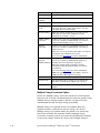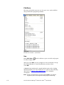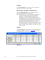
1
Particle Sizers Aerosol Instrument Manager® Software for Scanning Mobility Particle Sizer™ (SMPS™) Spectrometer User’s Manual P/N 1930038, Revision H April 2010 Aerosol Instrument Manager® Software for Scanning Mobility Particle Sizer™ (SMPS™) Spectrometer Introduction 1 Installing the Software 2 Getting Started 3 SMPS™ Procedures 4 User’s Manual Appendixes Manual History The following is a manual history of the Aerosol Instrument Manager Software for Scanning Mobility Particle SizerTM (SMPSTM) Spectrometer User’s Manual (Part Number 1930038). ii Revision Date First Version A B C D E F G H May 2002 October 2002 May 2004 February 2005 November 2005 March 2006 April 2006 October 2006 April 2010 Warranty Part Number Copyright Address Email Address World Wide Web Site Telephone No. Fax No. 1930038 / Revision H / April 2010 Limitation of Warranty and Liability (effective July 2000) Seller warrants the goods sold hereunder, under normal use and service as described in the operator's manual, shall be free from defects in workmanship and material for twelve (12) months, or the length of time specified in the operator's manual, from the date of shipment to the customer. This warranty period is inclusive of any statutory warranty. This limited warranty is subject to the following exclusions: ©TSI Incorporated / 2002–2010 / All rights reserved. TSI Incorporated / 500 Cardigan Road / Shoreview, MN 55126 / USA [email protected] http://www.tsi.com/ 1-800-874-2811 (USA only) or (651) 490-2811 (651) 490-3824 a. Hot-wire or hot-film sensors used with research anemometers, and certain other components when indicated in specifications, are warranted for 90 days from the date of shipment. b. Parts repaired or replaced as a result of repair services are warranted to be free from defects in workmanship and material, under normal use, for 90 days from the date of shipment. c. Seller does not provide any warranty on finished goods manufactured by others or on any fuses, batteries or other consumable materials. Only the original manufacturer's warranty applies. d. Unless specifically authorized in a separate writing by Seller, Seller makes no warranty with respect to, and shall have no liability in connection with, goods which are incorporated into other products or equipment, or which are modified by any person other than Seller. The foregoing is IN LIEU OF all other warranties and is subject to the LIMITATIONS stated herein. NO OTHER EXPRESS OR IMPLIED WARRANTY OF FITNESS FOR PARTICULAR PURPOSE OR MERCHANTABILITY IS MADE. TO THE EXTENT PERMITTED BY LAW, THE EXCLUSIVE REMEDY OF THE USER OR BUYER, AND THE LIMIT OF SELLER'S LIABILITY FOR ANY AND ALL LOSSES, INJURIES, OR DAMAGES CONCERNING THE GOODS (INCLUDING CLAIMS BASED ON CONTRACT, NEGLIGENCE, TORT, STRICT LIABILITY OR OTHERWISE) SHALL BE THE RETURN OF GOODS TO SELLER AND THE REFUND OF THE PURCHASE PRICE, OR, AT THE OPTION OF SELLER, THE REPAIR OR REPLACEMENT OF THE GOODS. IN NO EVENT SHALL SELLER BE LIABLE FOR ANY SPECIAL, CONSEQUENTIAL OR INCIDENTAL DAMAGES. SELLER SHALL NOT BE RESPONSIBLE FOR INSTALLATION, DISMANTLING OR REINSTALLATION COSTS OR CHARGES. No Action, regardless of form, may be brought against Seller more than 12 months after a cause of action has accrued. The goods returned under warranty to Seller's factory shall be at Buyer's risk of loss, and will be returned, if at all, at Seller's risk of loss. Buyer and all users are deemed to have accepted this LIMITATION OF WARRANTY AND LIABILITY, which contains the complete and exclusive limited warranty of Seller. This LIMITATION OF WARRANTY AND LIABILITY may not be amended, modified or its terms waived, except by writing signed by an Officer of Seller. Service Policy Knowing that inoperative or defective instruments are as detrimental to TSI as they are to our customers, our service policy is designed to give prompt attention to any problems. If any malfunction is discovered, please contact your nearest sales office or representative, or call TSI at 1-800-874-2811 (USA) or (651) 490-2811. iii Software License (effective March 1999) 1. GRANT OF LICENSE. TSI grants to you the right to use one copy of the enclosed TSI software program (the “SOFTWARE”), on a single computer. You may not network the SOFTWARE or otherwise use it on more than one computer or computer terminal at the same time. 2. COPYRIGHT. The SOFTWARE is owned by TSI and is protected by United States copyright laws and international treaty provisions. Therefore, you must treat the SOFTWARE like any other copyrighted material (e.g., a book or musical recording) except that you may either (a) make one copy of the SOFTWARE solely for backup or archival purposes, or (b) transfer the SOFTWARE to a single hard disk provided you keep the original solely for backup or archival purposes. 3. OTHER RESTRICTIONS. You may not rent or lease the SOFTWARE, but you may transfer the SOFTWARE and accompanying written material on a permanent basis, provided you retain no copies and the recipient agrees to the terms of this Agreement. You may not reverse-engineer, decompile, or disassemble the SOFTWARE. 4. DUAL MEDIA SOFTWARE. If the SOFTWARE package contains multiple types of media, then you may use only the media appropriate for your single-user computer. You may not use the other media on another computer or loan, rent, lease, or transfer them to another user except as part of the permanent transfer (as provided above) of all SOFTWARE and written material. 5. U.S. GOVERNMENT RESTRICTED RIGHTS. The SOFTWARE and documentation are provided with RESTRICTED RIGHTS. Use, duplication, or disclosure by the Government is subject to the restrictions set forth in the “Rights in Technical Data and Computer Software” Clause at 252.227-7013 and the “Commercial Computer Software - Restricted Rights” clause at 52.227-19. 6. LIMITED WARRANTY. TSI warrants that the SOFTWARE will perform substantially in accordance with the accompanying written materials for a period of ninety (90) days from the date of receipt. 7. CUSTOMER REMEDIES. TSI’s entire liability and your exclusive remedy shall be, at TSI’s option, either (a) return of the price paid or (b) repair or replacement of the SOFTWARE that does not meet this Limited Warranty and which is returned to TSI with proof of payment. This Limited Warranty is void if failure of the SOFTWARE has resulted from accident, abuse, or misapplication. Any replacement SOFTWARE will be warranted for the remainder of the original warranty period or thirty (30) days, whichever is longer. 8. NO OTHER WARRANTIES. TSI disclaims all other warranties, either express or implied, including, but not limited to implied warranties of merchantability and fitness for a particular purpose, with regard to the SOFTWARE and the accompanying written materials. 9. NO LIABILTY FOR CONSEQUENTIAL DAMAGES. In no event shall TSI be liable for any damages whatsoever (including, without limitation, special, incidental, consequential or indirect damages for personal injury, loss of business profits, business interruption, loss of information or any other pecuniary loss) arising out of the use of, or inability to use, this SOFTWARE. Trademarks Aerosol Instrument Manager is a registered trademark of TSI Incorporated. Scanning Mobility Particle Sizer and SMPS are trademarks of TSI Incorporated. Microsoft, Windows, Windows Vista, Access, and Excel are registered trademarks of Microsoft Corporation. iv Aerosol Instrument Manager® Software for SMPSTM Spectrometer Contents Manual History .......................................................................................... ii Warranty ................................................................................................... iii Software License (effective March 1999) ........................................... iv Trademarks .......................................................................................... iv About This Manual .................................................................................. xi Purpose ................................................................................................ xi Related Product Literature ................................................................... xi Getting Help ......................................................................................... xi Submitting Comments ......................................................................... xii CHAPTER 1 Introduction ...................................................................... 1-1 How This Manual is Organized ......................................................... 1-2 Notations/Conventions Used in This Manual .................................... 1-2 CHAPTER 2 Installing the Software..................................................... 2-1 Installation Requirements ................................................................. 2-1 Installation ......................................................................................... 2-2 CHAPTER 3 Getting Started ................................................................. 3-1 Start the Program .............................................................................. 3-1 Open an Existing File ........................................................................ 3-2 Change Data Display ........................................................................ 3-3 Display Another Sample in the Same File ........................................ 3-4 Playback (Review) Data Samples..................................................... 3-4 Select a Data Hot Spot ..................................................................... 3-6 Delete/Undelete Samples ................................................................. 3-6 Zoom In and Out on Data in a Graph ............................................... 3-7 Print Information Displayed on the Desktop ..................................... 3-8 Export Data to a File ......................................................................... 3-9 To Export Data to a File Manually ................................................. 3-9 To Export Data to a File Automatically ........................................ 3-11 Arrange Open Windows .................................................................. 3-12 Quit the Program ............................................................................. 3-13 CHAPTER 4 SMPS™ Spectrometer Procedures ................................ 4-1 How To Collect Sample Data ............................................................ 4-1 Step A: Open a New SMPS™ File ................................................ 4-1 Step B: Review/Change/Setup SMPS™ Properties ...................... 4-4 Step C: Start Data Collection ......................................................... 4-5 Setting Up Properties for an SMPS™ Spectrometer ........................ 4-6 SMPS™ Hardware Settings Tab ................................................... 4-6 SMPS™ Scheduling Tab ............................................................. 4-10 SMPS™ Physical Properties Tab ................................................ 4-12 SMPS™ Communications Tab .................................................... 4-16 v Append Sample Data to an Existing SMPS™ File ......................... 4-17 Export SMPS™ Data to an Access Database ................................ 4-18 To Set Up the Database .............................................................. 4-18 To Export Data to the Database .................................................. 4-19 Database Tables .......................................................................... 4-20 Active Menus for an SMPS™ Spectrometer ................................... 4-21 File Menu ..................................................................................... 4-22 Run Menu .................................................................................... 4-26 Playback Menu ............................................................................ 4-28 Format Menu ............................................................................... 4-29 View Menu ................................................................................... 4-35 Sample Menu ............................................................................... 4-43 Window Menu .............................................................................. 4-44 Help Menu.................................................................................... 4-45 Status Bar Icons .............................................................................. 4-46 APPENDIX A Data Files, Project Files, and Stored Parameters ...... A-1 Data Files and Project Files .............................................................. A-1 Project File Parameters .................................................................... A-2 Saved Parameters ............................................................................ A-3 APPENDIX B Accelerator Keys ........................................................... B-1 APPENDIX C Calculations Used for SMPS TM Spectrometer ............ C-1 APPENDIX D SMPS™ Software Comparison .................................... D-1 APPENDIX E Sequence Files ............................................................... E-1 Opening a File That is Part of a Sequence ....................................... E-2 APPENDIX F Error Messages ............................................................... F-1 APPENDIX G Scanning Mobility Particle Sizer™ (SMPS™) Spectrometer Diffusion Loss Correction .............................. G-1 Why Are Diffusion Losses Important in the SMPS™ spectrometer? ............................................................................... G-1 How Can You Characterize Diffusion Losses in the SMPS™ spectrometer? ............................................................................... G-2 Determination of P1 ....................................................................... G-3 Determination of P2 ....................................................................... G-3 Determination of P3 ....................................................................... G-4 Determination of P4 ....................................................................... G-4 Determination of P5 ....................................................................... G-4 How Does It Work? .......................................................................... G-4 When Should I Use Diffusion Loss Correction?............................... G-6 Ultrafine Particles .......................................................................... G-6 Low Flow Rates ............................................................................ G-6 Free Upgrade ................................................................................... G-6 References ....................................................................................... G-7 vi Aerosol Instrument Manager® Software for SMPSTM Spectrometer APPENDIX H Scanning Mobility Particle Sizer™ (SMPS™) Spectrometer Nanoparticle Aggregate Mobility Analysis Software Module ...................................................... H-1 Introduction ...................................................................................... H-1 Theory .............................................................................................. H-2 Assumptions – Limiting Case of Idealized Aggregates ................ H-2 Calculations .................................................................................. H-3 Module 1: Aggregate Drag ............................................................... H-4 Module 2: Charging Efficiency ......................................................... H-5 Number, Surface and Volume Distribution of Aggregates............ H-6 Software Operation .......................................................................... H-6 Example ........................................................................................ H-8 Summary and Conclusions .............................................................. H-9 References ....................................................................................... H-9 APPENDIX I Communication with the Electrostatic Classifier Model 3080 ................................................................................. I-1 Index Reader’s Comments Figures 3-1 3-2 3-3 3-4 3-5 3-6 3-7 The Aerosol Instrument Manager® Desktop and Selected Displays ........................................................................................... 3-2 Playback Setup Dialog Box ............................................................. 3-5 Use the Mouse to Directly View Data Values .................................. 3-6 Print Preview .................................................................................... 3-8 The Export Parameters Box. ........................................................... 3-9 A Sample Export File for an SMPS™ Spectrometer .....................3-10 Two-Pane Layout of an SMPS™ File ............................................3-12 4-1 4-2 Select an SMPS™ Filename When you Open a New File ..............4-2 CLASSIFIER Model 3080 Communications Port Selection Screen.............................................................................................. 4-3 4-3 Unable to Establish a Connection to the CPC Error Message ........4-4 4-4 Hardware Settings Tab of the Properties Dialog .............................4-7 4-5 Scheduling Tab of the Properties Dialog for an SMPS™ Spectrometer ................................................................................. 4-11 4-6 Physical Properties Tab of the SMPS™ Properties Dialog ...........4-13 4-7 The Communications Tab of the Properties Dialog .......................4-17 4-8 File Menu for an SMPS™ Spectrometer .......................................4-22 4-9 Run Menu for an SMPS™ Spectrometer ......................................4-26 4-10 Playback Menu .............................................................................. 4-28 4-11 Format Menu for an SMPS™ File (A) When a Graph Window is Active (B) When a Samples List Window is Active ....................4-30 4-12 The Y-Axis Dialog Box ................................................................... 4-30 4-13 View Boundaries Dialog Box ......................................................... 4-31 Contents vii 4-14 (A) The Graph Color Dialog Box, (B) The Table Color Dialog Box ................................................................................................. 4-33 4-15 The Font Dialog Box ...................................................................... 4-34 4-16 View Menu for an SMPS™ Spectrometer .....................................4-35 4-17 Units Selection Menu ..................................................................... 4-35 4-18 Electrical Mobility Diameter Data Displayed in %Concentration ...4-37 4-19 Weight Menu .................................................................................. 4-37 4-20 Size Data Weighted by Mass......................................................... 4-39 4-21 4-22 4-23 4-24 4-25 4-26 4-27 Statistics Table .............................................................................. 4-40 Select Settings to Display SMPS™ Settings for the Sample ........4-41 Sample Menu ................................................................................. 4-43 Window Menu ................................................................................ 4-44 Help Menu...................................................................................... 4-45 Status Bar Displaying Particle Density ..........................................4-46 Status Bar Displaying Dashed Lines .............................................4-46 E-1 File Question? Dialog Box .............................................................. E-2 G-1 Circular Tube Penetration Efficiency [Gormley and Kennedy (1949)] ............................................................................. G-2 Schematic of the Component Scanning Mobility Particle Sizer™ Spectrometer ..................................................................... G-3 SMPS™ Properties Box Screen of Aerosol Instrument Manager® Software for the SMPS™ Spectrometer ........................ G-5 Aerosol Instrument Manager Data file of Outdoor Air without Diffusion Loss Correction................................................................ G-6 Aerosol Instrument Manager Data file of Outdoor Air with Diffusion Loss Correction................................................................ G-6 G-2 G-3 G-4 G-5 H-1 H-2 H-3 viii Two Module Approach for Nanoparticle Aggregate Mobility Analysis. Courtesy: Lall, et al., 2006 c ........................................... H-3 Physical Properties Tab of the Aerosol Instrument Manager® Software Showing the Nanoparticle Aggregate Mobility Analysis Module User Interface. ..................................................... H-7 Aggregate distribution functions based on standard calibration for spheres (Red) compared with the distributions based on the idealized aggregate theory (Green). Primary particle diameter = 17 nm, aggregate orientation: parallel to the electric field. (a) Number Distributions, (b) Surface area distributions and (c) Volume distributions. Courtesy: Lall et al., 2006 c. ................... H-8 Aerosol Instrument Manager® Software for SMPSTM Spectrometer Tables 4-1 4-2 4-3 4-4 4-5 4-6 Descriptions for SMPS™ Hardware Settings Tab .......................... 4-7 Descriptions for the SMPS™ Scheduling Tab .............................. 4-11 Descriptions of the SMPS™ Physical Properties Tab .................. 4-13 Descriptions for the Communications Tab .................................... 4-17 Display Options for Units ............................................................... 4-36 Weight Options .............................................................................. 4-38 F-1 Error Messages for SMPS™ Spectrometer .................................... F-1 Contents ix (This page intentionally left blank) x Aerosol Instrument Manager® Software for SMPSTM Spectrometer About This Manual Purpose This is an instruction manual for the Aerosol Instrument Manager® Software as it applies to a TSI Scanning Mobility Particle Sizer™ (SMPS™) Spectrometer. Related Product Literature Model 3934 Scanning Mobility Particle Sizer™ (SMPS™) Spectrometer manual, part number 1930081, TSI Incorporated Model 3936 Scanning Mobility Particle Sizer™ (SMPS™) Spectrometer manual, part number 1933796, TSI Incorporated Model 3980C macroIMS™ Macroion Mobility Spectrometer manual, part number 1930110, TSI Incorporated Model 390069 Data Merge Software Module manual, part number 1930074, TSI Incorporated Series 3080 Electrostatic Classifiers manual, part number 1933792, TSI Incorporated Getting Help To obtain assistance for this software or to submit suggestions, please contact Particle Instruments: TSI Incorporated 500 Cardigan Road Shoreview, MN 55126 USA Fax: (651) 490-3824 Telephone: 1-800-874-2811 (USA) or (651) 490-2811 E-mail: [email protected] xi Submitting Comments TSI values your comments and suggestions on this manual. Please use the comment sheet, on the last page of this manual, to send us your opinion on the manual’s usability, to suggest specific improvements, or to report any technical errors. If the comment sheet has already been used, mail or fax your comments on another sheet of paper to: TSI Incorporated Particle Instruments 500 Cardigan Road Shoreview, MN 55126 Fax: (651) 490-3824 E-mail Address: [email protected] xii Aerosol Instrument Manager® Software for SMPSTM Spectrometer CHAPTER 1 Introduction The Aerosol Instrument Manager® software is used to collect sample data from a spectrometer and store the sample data in files. You can use the software to display data in graphs and tables, or view statistical information. You can print graphs and tables with the software, and you can export data for use in other applications, including a Microsoft® Access® database. There are a number of ways to navigate within the program. These include selecting items from the main menus, selecting icons from the toolbar, and selecting items from submenus (which you access by right-clicking the mouse button). Specific instructions are provided in the following chapters. The Aerosol Instrument Manager® software is designed to be used with a variety of different TSI spectrometers and sensors. Aerodynamic Particle Sizer® (APSTM) Spectrometers Scanning Mobility Particle Sizer™ (SMPS™) Spectrometers Condensation Particle Counters (CPCs) Electrical Aerosol Detectors (EADs) Aerosol Electrometers Electrostatic Classifiers This manual covers the use of the Aerosol Instrument Manager® software with TSI Scanning Mobility Particle Sizer™ (SMPS™) Spectrometers only. For information about software operation with other TSI spectrometers and sensors, refer to the appropriate manual. This manual assumes you have Microsoft® Windows® XP, Windows Vista®, or Windows 7 (32-bit) on your computer and that you are familiar with how Windows® works. If you are not familiar with Windows® operation system, please refer to the information that came with it before you load and use this program. ® Microsoft, Windows, and Windows Vista are registered trademarks of Microsoft Corporation. 1-1 How This Manual is Organized This manual describes the Aerosol Instrument Manager® software and includes information such as: Requirements for loading and running the software. The installation procedure that loads the program onto your computer. A “Getting Started” chapter that introduces basic software operation. “How to...” information for using the program to operate and collect data with the SMPS™ spectrometer. Descriptions of the menus and menu items which are valid when collecting data with an SMPS™ spectrometer. Appendixes that provide reference information associated with program operation. Notations/Conventions Used in This Manual 1-2 Throughout this manual when reference is made to “Windows,” it implies either Windows® XP, Windows Vista®, or Windows 7 operating system. Bold face type is used to indicate that you should perform the indicated action. For example “select the File menu” means that you should use the mouse and click on the menu called File. When instructions direct you to select items from a menu, a vertical bar (|) is used to separate the items you should select. For example, “select File|Properties|Scheduling” means you should click on the File menu, then select the Properties item, and then select the Scheduling tab. The term “active window” is used to refer to the window that is open on the desktop and is in focus. To verify which window is active, select the Window menu and note which item has a checkmark by it. You can make a window active by moving the pointer to that window and clicking the mouse button. Aerosol Instrument Manager® Software for SMPSTM Spectrometer CHAPTER 2 Installing the Software This chapter describes the installation requirements for the Aerosol Instrument Manager® software and the installation procedure. Note: If the Data Merge software, is being used with the Aerosol Instrument Manager® software, it should be installed as listed: C:\Program Files\tsi\Data Merge Software Module\DataMerge.exe When installed correctly, Aerosol Instrument Manager® software activates the data merge software and the Data Merge icon appears ( ) on the main toolbar. For more information on the Data Merge software, please refer to the Model 390069 Data Merge Software Module manual (P/N 1930074). Installation Requirements To use this software we recommend a personal computer with the following minimum features, components, and software: A Pentium® 586 processor or higher. A SVGA color monitor. Microsoft Windows® XP, Windows Vista®, or Windows 7 (32-bit) operating system. A hard drive large enough to accommodate Windows®, the Aerosol Instrument Manager® software, and data files. Note: The amount of disk space required depends on the number of samples you collect, the amount of information collected, and the sampling period. After you have collected a number of samples, you may want to look at the file size to estimate how much storage space you will be using. ® ® A CD-ROM drive. Pentium is a registered trademark of Intel Corporation. Microsoft® Windows® are registered trademarks of Microsoft Corporation. 2-1 256 MB or more of random access memory (RAM). A mouse. An RS-232 serial interface port or a USB port for each instrument connected (in addition to the one that may be required for the mouse). USB connections are available for Series 3770 CPCs and Series 3780 particle counters. Note: Three Series 3770 CPCs can be connected using USB to collect data simultaneously. A Microsoft Windows® operating system-compatible printer is optional. Installation Install the Aerosol Instrument Manager® software as follows: 1. Shut down (exit) all programs/applications on the Windows® desktop. 2. With the computer on and Windows® operating system running, insert the Aerosol Instrument Manager® CD-ROM in your CD drive to run the autorun.exe from the CD. a. If AutoPlay is enabled on your PC, the setup program will begin automatically and the introduction screen is displayed on the Windows® desktop. b. If AutoPlay is not enabled, select Run from the Start menu and type: D:\autorun (where D is the letter corresponding to your CD drive) in the Open box and press OK. 3. Follow the instructions as the setup program runs. When setup is complete, you should read the readme.htm file. This file contains information that could not be included in this manual. If you decide not to read the file immediately, you can access the file later using a browser such as Windows® Internet Explorer® browser. 4. When the installation program finishes, remove the CD-ROM and store the CD in a safe place for later use. The setup program creates a directory (folder) called “Aerosol Instrument Manager” on your hard disk (assuming you accepted the default directory name). The directory contains the required program files and sample data files. The setup program also creates a new item in the Start Menu called “TSI” and an icon for the Aerosol Instrument Manager® software. Note: Before creating a TSI menu item, the setup program checks for an existing one. If one is present, it adds the icon only. 2-2 Aerosol Instrument Manager® Software for SMPSTM Spectrometer CHAPTER 3 Getting Started Aerosol Instrument Manager® software version 8.2 includes support for the Model 3080 Electrostatic Classifier. If the classifier is connected to the computer via an RS-232 cable, the software will read temperature and pressure from the classifier and use those values to calculate gas viscosity and mean free path. If the software is not connected to the classifier, the reference values entered on the SMPS™ Properties dialog will be used. The software will also set the sheath flow rate and bypass flow rate in the classifier to the values selected on the SMPS™ Properties dialog. This chapter is designed to give you an introduction to the basic operation of the Aerosol Instrument Manager® software. Using it, you will: Start the program. Open an existing file (from the example files provided with the program). Change data display. Display another sample in the same file. Playback (review) data samples in a “slide show” fashion. Select a data hot spot. Delete/Undelete samples. Zoom in and zoom out on data in a graph. Print information displayed on the desktop. Export data to a file. Arrange open windows. Quit the program. Start the Program To start the program, proceed as follows: From the Windows® desktop, using the mouse, double-click the Aerosol Instrument Manager® icon or press the Start menu and then select Programs|TSI|Aerosol Instrument Manager. 3-1 The Aerosol Instrument Manager® desktop appears as shown in Figure 3-1. Data Display: Graph Format Data Display: Table Format Menu Options Tool Bar Instrument Settings Sample List Data Statistics Instrument Settings Figure 3-1 ® The Aerosol Instrument Manager Desktop and Selected Displays Open an Existing File 1. Select File|Open…or on the toolbar. The “Open Instrument Associated Data Files” window opens. 2. When the “Open Instrument Associated Data Files” window appears, select the correct extension for the file you want to open in the “Files of type” box. For example, for an SMPS™ spectrometer, the file extension is .s80. If necessary, browse for the drive/directory where data files are stored. (Example files are included with the program and were 3-2 Aerosol Instrument Manager® Software for SMPSTM Spectrometer installed in the Aerosol Instrument Manager® folder when the program was installed.) 3. Select the data file that you want to open and click Open. At least two windows open on the desktop: a window containing a graph of the sample data, and the Samples List window (Figure 3-1). Note: If the file has been opened before, it may display more than one graph and/or table. The program remembers the windows that were open on the desktop when you last closed the file and reopens them when you access the file again. If the file contains a sequence of samples, you will be asked if you want to open all the files or just the one you originally chose. See Appendix E for information about sequence files. The Samples List window opens whenever you open a data file and remains open on the desktop as long as the data file is open. Closing the Samples List window closes the data file (and all its open windows). Change Data Display For most spectrometers, you can view data in tables or graphs and in several different formats (for example, SMPS™ data can be viewed by raw counts, concentration, and so on). The following procedure provides an example of how you can change data display. 1. Open one of the sample SMPS™ files as described in “Open an Existing File”. With the graph window active on the desktop, point and the mouse on the graph, right-click the mouse to display various viewing options. Refer to “Format Menu” in Chapter 4 for detailed explanations. Notice the change in how data is displayed. (A checkmark next to one of the menu items means that a window for that selection is already open on the desktop. If you select a menu item that is already checked, the window containing that graph or table is brought to the top of the desktop and becomes the active window.) 2. Experiment with other views by making other windows active and selecting other options from the View menu to see how your selections change the data display. Getting Started 3-3 Display Another Sample in the Same File 1. To display another sample in an open file, select the icon (go forward one sample) from the toolbar. The data for the next sample of the currently active file replaces the data in all the open windows. 2. You can continue to step through the samples by selecting the icon until you reach the last sample. The sample currently displayed in the open window is highlighted in the Samples List window. Another method of changing the sample that is displayed in the open windows on the desktop is by selecting the icon for that sample from the active Samples List window. You can use the following icons to display other samples: First Sample. Advance to the first sample. Previous Sample. Go back to the previous sample. Next Sample. Advance to the next sample. Last Sample. Advance to the last sample. Playback (Review) Data Samples You can display sample graphs and tables in a slide show format (to preview sample results or compare sample differences) as follows: 1. From the Samples List window, select the samples you want to play back using one of the following actions: Select Sample|Select All, to play back all samples. or Select individual samples using the mouse and the Ctrl key to highlight those samples you want to see. (You must select at least two samples.) or Select a group of samples by holding down the left mouse button and moving the mouse to “rubber band” (outline) the samples you want to select. Note: The Playback menu items and toolbar icons are only enabled when the Samples view is the active view. 3-4 Aerosol Instrument Manager® Software for SMPSTM Spectrometer 2. When you have selected the samples you want to view, select Playback|Play. The setup box shown in Figure 3-2 appears. Figure 3-2 Playback Setup Dialog Box 3. Select the sample viewing time and whether you want the samples displayed once or continuously. Playback begins immediately. For better viewing, it may be necessary to minimize the Samples List window. 4. Playback can be paused at any time by selecting Playback|Pause. Select Playback|Play to continue playback where you left off. Playback can be stopped at any time by selecting Playback|Stop. When playback is stopped, you cannot restart it. Use Playback|Pause and Playback|Play if you want to stop and start playback. You can also control playback by using icons on the toolbar. The icons perform the following operations: Stop. Stop playback. Pause. Pause playback on current sample. Start. Start playback or restart playback. Getting Started 3-5 Select a Data Hot Spot When a graph is open on the desktop, you can find the values of a data point as follows: 1. Position the pointer on the bar, line, or peak (depending on the type of graph that is active). The pointer becomes a pointing hand. 2. Press the left mouse button to display the values. Figure 3-3 shows how the data values would be displayed for an SMPS™ spectrometer (diameter and number concentration). Figure 3-3 Use the Mouse to Directly View Data Values Tip: After you have a data hot spot selected, use the arrow keys or the “>“ and “<“ keys to move the cursor right or left (from one value to the next), or grab the vertical bar and drag it to another location. Refer to Appendix B for a list of other keys or key combinations you can use to navigate and perform operations without using the mouse. Delete/Undelete Samples To delete samples from a file, you must first mark them for deletion and then either Close or Save the file. The following procedures will permanently delete samples from a file: Mark samples for deletion as follows: 1. Select the sample you want to delete from the Samples List window (you can select multiple samples). 3-6 Aerosol Instrument Manager® Software for SMPSTM Spectrometer 2. Select Sample|Delete/Undelete Sample or on the toolbar. The samples will be shown as “Deleted.” However, they will not be permanently removed from the file until you Close or Save the file. Save the file and permanently delete all samples marked for deletion: 1. With at least one sample marked for deletion in the active file, select File|Save. You will get a message stating: “Some samples have been marked for deletion. Do you want them permanently removed?” Click Yes to remove them or No to keep them. 2. Select Yes. The samples marked for deletion are permanently deleted. Note: If you attempt to close all the windows for the file or exit the program without saving the file, you will get a message asking whether you want to save changes to the file. Respond Yes and you will get the same message stating “Some samples have been marked for deletion. Do you want them permanently removed?” Respond Yes to delete the marked samples and No to close the file without deleting them. Zoom In and Out on Data in a Graph You can zoom in on data displayed in a graph as follows: 1. Use the mouse to position the cursor (pointer) at one corner of the area you want enlarged. 2. Press down on the left mouse button and drag the mouse to the opposite corner of the data you want enlarged. 3. Release the left mouse button. The area you selected is enlarged. 4. You can continue to zoom further by repeating steps 1 through 3. To Unzoom, select Format|Undo Zoom or enlarged area is returned to normal view. Getting Started on the toolbar. The 3-7 Print Information Displayed on the Desktop You can print the information displayed in the active window on the desktop as follows (you must have a printer properly installed): 1. With a graph or table window active on the desktop, select File|Print Preview or . 2. Review that what you see in the print preview window is what you want to print (an example is shown in Figure 3-4), and then select Print from the Preview box. The contents of the window are sent to your printer. You can immediately print a window without previewing it by selecting File|Print or from the toolbar. Figure 3-4 Print Preview 3-8 Aerosol Instrument Manager® Software for SMPSTM Spectrometer Export Data to a File You can export data from an SMPS™ Aerosol Instrument Manager® file (either a single sample of the file or multiple samples of the file) for use in another program such as Microsoft Excel® or Microsoft Access® database. You can export data either manually or automatically. Refer to Chapter 4 for information on exporting SMPS™ data to the database. To Export Data to a File Manually To export data to be used in another program: 1. Select the sample or samples to be exported as follows: To export data from a single sample, display the sample data in an active window on the desktop. To export data from multiple samples, select (highlight) the samples you want to export from the Samples List window. 2. Select File|Export to File. An Export Parameters dialog box appears as shown in Figure 3-5. Figure 3-5 The Export Parameters Box. Getting Started 3-9 3. Select the type of data you want to export as well as the format you want to export the data in. Data can be exported in a delimited text file and you can select from three delimiters: tab, comma, or semicolon. The orientation of data can be either column or row. 4. Click OK. 5. Select the drive/directory you want to export the data to and enter a filename. The system automatically adds the .txt file extension. 6. Click Save. Figure 3-6 illustrates how an exported *.txt file is formatted for an SMPS™ spectrometer. Figure 3-6 A Sample Export File for an SMPS™ Spectrometer 3-10 Aerosol Instrument Manager® Software for SMPSTM Spectrometer To Export Data to a File Automatically To export data automatically to a file for use in another program (such as Microsoft® Excel®): 1. Establish a connection to the spectrometer by choosing File|New or File|Open. 2. If not already connected, select Run|Connect to the CPC. Note: Perform the following step before you start collecting the data. 3. Select Run|Auto Export to File. Select the type of data you want to export as well as the format you want to export the data in, using the Export Parameters dialog box (see Figure 3-5 on previous page). 4. Select Run|Start Data Collection. The data is exported to the file as it is collected. (continued on next page) ® Microsoft and Excel are registered trademarks of Microsoft Corporation. Getting Started 3-11 Arrange Open Windows When you have several windows open on the desktop it is helpful to arrange them for easier viewing. To arrange windows, select an item from the Window menu. You can arrange windows on your desktop horizontally, vertically, have them cascade, or arrange them in a predetermined auto-fit 2-pane or 4-pane layout. Refer to your Windows® documentation for examples and more information for tile horizontal, tile vertical, and cascade layouts. Press the button (or Ctrl+L) in the toolbar for the four-pane layout or press the button (or Ctrl+K) for the twopane layout as shown in Figure 3-7 for a spectrometer file. Figure 3-7 Two-Pane Layout of an SMPS™ File All of the program windows that are currently open on the desktop are listed at the bottom of the Window menu under the Close All item. To make a window active and bring it to the top of all windows, select the name of the window from the list of open windows. 3-12 Aerosol Instrument Manager® Software for SMPSTM Spectrometer Quit the Program To end the program, select File|Exit. All windows and files open on the desktop are closed. If you have made changes to a file and have not yet saved it, you will be prompted to do so. Getting Started 3-13 (This page intentionally left blank) 3-14 Aerosol Instrument Manager® Software for SMPSTM Spectrometer CHAPTER 4 S M P S™ S p e c t r o m e t e r Procedures Before using the information in this chapter, read Chapter 3. That chapter provides getting started information to help you understand the basics of how the program works. It also includes procedures common to all spectrometers. The subsections of this chapter provide: “How To...” information for: collecting sample data with an SMPS™ spectrometer, setting up properties for an SMPS™ spectrometer, appending sample data to an existing SMPS™ file, exporting SMPS™ data to a Microsoft Access® database. A description of all menus and menu items available when using the SMPS™ spectrometer or viewing SMPS™ data files. How To Collect Sample Data There are three steps for collecting sample data. Step A: Open a new SMPS™ file Step B: Review/change parameters Step C: Start data collection Note: You can append SMPS™ sample data to an existing file. Refer to “Append Sample Data to an Existing SMPS™ File” below. Before you begin, make certain you have connected the CPC to the computer and the spectrometer is running. Refer to the appropriate hardware instruction manual if necessary. Step A: Open a New SMPS™ File To open a new SMPS™ File: on the toolbar. The New Instrument and 1. Select File|New or Associated Data File dialog box (Figure 4-1) opens on your desktop. 4-1 Figure 4-1 Select an SMPS™ Filename When you Open a New File Note: The following step must be performed before you start collecting data. 2. Select a filename (and, optionally, a location other than the Aerosol Instrument Manager® folder). The default name is “AIM1” for the first file you open, “AIM2” for the second file you open and so on. You can accept the default name or enter any name you choose. 3. Verify that the “Files of Type” box indicates the correct extension for the spectrometer you are using (.S80 for an SMPS™ spectrometer). You do not need to enter an extension in the filename box. It is assigned automatically. 4. Click the Open button. 4-2 Aerosol Instrument Manager® Software for SMPSTM Spectrometer 5. If the Model 3080 Classifier is currently selected and autoconnect is selected, the software will attempt to connect to the classifier at this time, first using the current default COM port selection for this instrument and next trying the other available Com ports. If the attempt to connect fails, the CLASSIFIER Model 3080 Communications dialog will appear allowing you to select the COM port (Figure 4-2). This is separate from the dialog that allows you to select the COM port for the CPC. That dialog is found on the Communications page of the Properties dialog 6. You can select the correct port by double-clicking on the port name (e.g., COM1), or click the Cancel button if not using the Model 3080 Classifier, or if planning to run the software without connecting to the classifier (Figure 4-2). In the latter case, you will need to set the flow and other values on the classifier manually and the software will use reference gas values from the Properties dialog rather than values read from the classifier. Figure 4-2 CLASSIFIER Model 3080 Communications Port Selection Screen Note: The Communications page on the Properties dialog is for selecting a port for connection to the Condensation Particle Counter, not the Classifier. You can use the menu to connect to the Model 3080 Classifier, by selecting Run | Connect to Classifier 3080. 7. If you open a new file and the SMPS™ Properties dialog is not complete (this can occur the first time you open a new file for the SMPS™ spectrometer or after you have selected File|Clear SMPSTM Spectrometer Procedures 4-3 Settings) the SMPS™ Properties dialog box appears and you must complete it and press OK to proceed. 8. If you get the following error message when opening a New file, press the OK button to open the Properties dialog box (Figure 4-3). Figure 4-3 Unable to Establish a Connection to the CPC Error Message 9. Verify the connection to the spectrometer and make certain the spectrometer is turned on. To verify the COM or USB Port setting: a. Check that the correct communications port was selected during program setup by double-clicking on the port listed under the Communications Tab. b. If the test is unsuccessful, select another port and double click on the port again. Note: The new Series 3770 Condensation Particle Counters have USB ports to connect to the computer. The Series 3780 Water-based Condensation Particle Counters also have USB ports but they are treated as serial ports using a USB driver. See instrument manual for details. c. Once the correct port is selected, select OK to return to the desktop and the active window. Step B: Review/Change/Setup SMPS™ Properties Before you begin sampling, you may want to review the Properties dialog to verify correct start time, hardware settings, and so on. 1. Select File|Properties or Run|Properties (or Ctrl+R) and select the various tabs to review the settings. Refer to “Setting Up Properties for an SMPS™ Spectrometer” for how to change settings. 2. If the software is connected to the Model 3080 Classifier, the temperature and pressure read from the classifier are used to calculate mean free path and gas viscosity and these values are 4-4 Aerosol Instrument Manager® Software for SMPSTM Spectrometer used in calculations. If not connected to the Model 3080 Classifier, the reference gas values from the Physical Properties page of the SMPS™ Properties dialog are used instead. 3. Once you have set up the parameters or verified they are correct, close the Properties dialog box and continue with Step C, “Start Data Collection.” 4. At this time, if connected to the Model 3080 Classifier, the software will set the sheath flow rate and bypass flow rate in the classifier to the values selected on the properties dialog. It will also set the sheath flow mode to the appropriate value (dual or single blower) based on the flow selections, and will set voltage mode to analog. The software will also set the CPC flow rate to the selected high or low value when the CPC has two flow modes. Step C: Start Data Collection After you have completed the properties dialog, data collection begins at the “Start At Time” you set on the Properties dialog or immediately after you do one of the following: Select Run|Start Data Collection using the menus. Click Double-click the New Sample icon in the Samples List window. on the toolbar. If the model 3080 classifier has been selected, the software will read the sheath temperature and absolute pressure from the classifier and will wait for OK status from the classifier before it starts to collect data. The software displays the temperature and pressure at the bottom of the graph and tables. If the software is not connected to the classifier or unable to read from it, there will be dashed lines at the bottom of the graph and tables in place of the temperature and pressure. When the program begins collecting sample data, the data is displayed in the windows that are open on the desktop. As each sample finishes, the data for the sample is stored and a new sample begins. When the last sample finishes, sampling stops, but the windows remain open. To stop data collection before all the samples are collected, do one of the following: Select Run|Finish Current Sample. Data collection stops after the current sample finishes. or SMPSTM Spectrometer Procedures 4-5 Select Run|Abort Current Sample or on the toolbar to stop data collection immediately. When you select Abort Current Sample, the data collected for the current incomplete sample is discarded. S e t t i n g U p P r o p e r t i e s f o r a n S M P S™ Spectrometer To access the Properties dialog box for an SMPS™ spectrometer, select File|Properties or Run|Properties (or Ctrl+R) when an SMPS™ file is active on the desktop. The properties displayed in the Properties dialog box are either: The initial default properties as set by TSI or The default properties set by a user who selected File|Save Properties as Default after making changes to the Properties dialog box or changed the settings and had the File|Save Properties on Exit menu item checked. The Properties dialog box contains four tabs: Hardware Settings, Scheduling, Physical Properties, and Communications. Each is described below. If this is the first time you have accessed the Properties dialog, you will need to set up the parameters before continuing. If you have set up the properties before, verify they are correct and press OK. The following paragraphs describe the settings for each tab of the Properties dialog box. Note: If you want to use the same settings the next time you open a new file, remember to either select File|Save Settings As Default or have the File|Save Settings on Exit menu item checked after you have completed the Properties dialog. Once your settings have been saved, the properties dialog will not open automatically when you open a new file. Some properties of an existing sample can be changed through the Properties dialog. If a common property of multiple samples needs to be changed, you can first select the samples and then access the Properties dialog to change the property of all the selected samples. SMPS™ Hardware Settings Tab Use the Hardware Settings tab to specify hardware settings for the SMPS™ spectrometer. The fields on the tab vary depending on the 4-6 Aerosol Instrument Manager® Software for SMPSTM Spectrometer model of classifier and the Differential Mobility Analyzer (DMA) model of your SMPS™ spectrometer. Figure 4-4 illustrates the tab for the Model 3080 Classifier with a 3085 Nano DMA. Table 4-1 describes each of the fields/settings. You cannot close the Properties dialog or select any of the other tabs until all values have been set on the Hardware Setting tab. Figure 4-4 Hardware Settings Tab of the Properties Dialog Table 4-1 Descriptions for SMPS™ Hardware Settings Tab Setting Description Classifier Model Select the model of Electrostatic Classifier used in the system. SMPSTM Spectrometer Procedures 4-7 Setting Auto-connect DMA Model HV Polarity Impactor Type CPC Model and Flow Rate Inlet Flow Rate (L/min) Aerosol Flow Rate (L/min) Sheath Flow Rate (L/min) Bypass Flow td (s) 4-8 Description Check this box if you want the software to automatically connect to the classifier by searching the ports to find the instrument. You can also select Run | Connect to Classifier from the menu. Select the model of Differential Mobility Analyzer used in the system. This is the polarity of the high voltage controller which is installed on your 3080 classifier. A negative high voltage controller is the default configuration and is used to measure positivelycharged particles with your SMPS™ spectrometer, Your selection must match the polarity of the high voltage controller physically installed in your 3080. According to your selection, the Aerosol Instrument Manager® software will read the appropriate charge correction file (ChargeAim.dat for negative high voltage controller or ChargePos.dat for positive high voltage controller) and apply this to your data. Note: Do not change this setting without physically changing the high voltage controller installed in your 3080! Refer to the 3080 manual on how to order a positive high voltage controller and how to install it. Select the type of impactor used in the system. Select the Condensation Particle Counter used in the system and the high or low flow rate for Condensation Particle Counter models 3022A, 3025A, 3775, and 3776 and for Water-based Condensation Particle Counter Models 3787 and 3788. Each model of Condensation Particle Counter differs in concentration range, sample flow rate, and other specifications. To avoid large errors in measured particle distributions, make sure the Condensation Particle Counter selected matches the one in your SMPS™ system. This option only appears when a Model 3022A Condensation Particle Counter with a high flow rate is selected. Enter the inlet flow rate of the Condensation Particle Counter. The value must be in the range 1 to 2. Enter the aerosol flow rate for the DMA. The value should be in the range .2 to 2.0. Enter the sheath flow rate for the DMA. The value should be in the range 2 to 20. Optional bypass flow in L/min. The use of bypass flow requires special flow plumbing. See the Classifier Model 3080 manual to set up the flow plumbing. If not using bypass flow, set this value to 0.0. td is the time for the aerosol to flow through the sample column of the classifier and the connection tubing between the DMA and the Condensation Particle Counter which is assumed to be 10 inches long. Although you can enter a value for td (0 to 10 seconds), it is recommended that you use the value calculated from the hardware settings. Aerosol Instrument Manager® Software for SMPSTM Spectrometer Setting tf (s) D50 (nm) Size Range Bounds (Diameter) Set to Max Range Voltage Range Scan Time Down Scan First Description The tab shows the tf (in seconds) of your SMPS™ spectrometer. tf is the calculated time for the aerosol to flow through the sample column of the classifier. The calculation of tf is based on the classifier’s sheath air flow rate, the polydisperse aerosol flow rate, and the geometry of the classifier. The tab shows the D50 cut point for the impactor at the inlet of your SMPS™ spectrometer. The D50 cut point is the 50% cut-point diameter of the impactor. It changes if you change the size of the impactor or the polydisperse aerosol flow rate. Enter the minimum and maximum size range to be sampled using the pull-down lists. The minimum and maximum size limits are determined by the DMA flow rates of your system. You can select the particle diameter range to view with this option, but choose new flow rates will change the available particle diameter sampling range. Select this button to automatically set the Size Range Bounds to the maximum range based on the current DMA and flow settings. Calculation is based on Max and Min voltages (vmin = 10 and vmax = 10,000 for the 3080 classifier; vmin = 10 and vmax =11,000 for the 3071 classifier). Displays the voltage range based on the size range selection. Enter the Scan Up and Scan Retrace times (in seconds). Scan Up time is the period during which the classifier center rod voltage is exponentially increasing in magnitude. Size distribution data is sampled during Scan Up. The Scan Up range is 20 to 300. At the start of the Scan Retrace time period, the classifier voltage is reset to its initial voltage. The Scan Retrace range is 10 to 300. Scan time selection depends on several factors including: desired particle size accuracy, CPC response time, flow rates, and particle size range. Generally, longer scan times provide better data, while decreasing the scan time results in a decrease of the particle size accuracy of the SMPS™ system. Accuracy decreases for three reasons: (1) smearing effects caused by the response time of the CPC, (2) the increased dependence on the exact value of td, and (3) the increase in granularity of the data. Typically, a 120-second Up Scan and a 15-second Retrace Scan (default values) provide adequate accuracy and are a good starting point. Use a shorter scan time (30 seconds) for measurements in which the aerosol changes substantially during the sample period. Use a longer scan time for measurements in which there is a low concentration and a high particle size accuracy is desired. Select this box to perform a down (retrace) scan first. The box is available only for the Classifier Model 3071. SMPSTM Spectrometer Procedures 4-9 Setting Cylindrical DMA Measurements (cm) Description These options are available only if you select the Custom DMA model. Enter the dimensions for your DMA. When the Model 3080 Electrostatic Classifier is selected and connected, the software reads the sheath temperature and the absolute pressure from the instrument and uses those values to calculate gas viscosity and mean free path, which are used in other calculations. If unable to read temperature and pressure from the instrument, the reference gas viscosity and mean free path from the properties dialog are used instead. The flow rates are not read from the classifier when the properties dialog is opened so the current flow values from the instrument are not displayed in the properties dialog. After you close the properties dialog the software sets the sheath flow and bypass flow rates in the Model 3080 Classifier to the values selected on the properties dialog. It also sets the CPC flow rate to the high or low value selected if the CPC has two flow rate options. SMPS™ Scheduling Tab Use the Scheduling tab to select: The number of scans per sample The number of samples to be taken How often samples are collected The start time for the first sample Figure 4-5 shows the Scheduling tab of the Properties dialog. Table 4-2 provides a description of each parameter. 4-10 Aerosol Instrument Manager® Software for SMPSTM Spectrometer Figure 4-5 Scheduling Tab of the Properties Dialog for an SMPS™ Spectrometer Table 4-2 Descriptions for the SMPS™ Scheduling Tab Parameter Description Scan Up Displays the value selected in the Hardware Settings tab. Retrace Displays the value selected in the Hardware Settings tab. Scans per Sample Enter the number of scans you want to take per sample. Number of Samples This is the total number of samples you want to collect. The maximum value allowed is 65535. Total Sample Time This field is calculated by the software and shows the total sample time based on the values you entered in the previous boxes. The value is displayed in hours, minutes, and seconds. Scheduled Select Only Once to collect one set of samples. For continuous monitoring, select Repeat Every and then select the hours and minutes between samples. The intersample time should be longer than the Total Sample Time to include the overhead time that is needed for file handling. SMPSTM Spectrometer Procedures 4-11 Parameter Start At Time Trigger File Description If you don’t check this box, sampling begins as soon as you select Start Data Collection. If you want to select a start time, check the box and enter the clock time at which you want sampling to begin. The program uses a 12-hour or 24-hour clock, depending on how your PC is set up. If your PC is set up to use a 12-hour clock, you must indicate if the time is am or pm by unchecking the PM box or checking the PM box. The reference time for the program is the time at which your computer is set. Specify a file name only (not a complete pathname) of a text file. This file when updated in the same directory where Aerosol Instrument Manager is installed, will act as a trigger to start SMPS™ sampling. For example, specify “trigger.txt” in the edit box. When you wish to trigger the sampling to begin, create or update the file trigger.txt in the Aerosol Instrument Manager directory (Note: the contents of this file are not read). Files of Sample Sessions That Run Past Midnight The files for sample sessions that run past midnight are handled differently than those that start and stop on the same date. In this case a sequence of files is created, with each file in the sequence given a unique filename identifying its proper order. Appendix E provides a complete description of sequence files including how to access a file that is part of a sequence. SMPS™ Physical Properties Tab Use the Physical Properties tab (Figure 4-6) to specify the physical properties of the sample, provide a title for the sample and enter any comments about the sample that you want to keep with the file. 4-12 Aerosol Instrument Manager® Software for SMPSTM Spectrometer Table 4-3 describes the fields of the Physical Properties tab. Figure 4-6 Physical Properties Tab of the SMPS™ Properties Dialog Table 4-3 Descriptions of the SMPS™ Physical Properties Tab Field Description Gas Viscosity Enter the gas viscosity of the gas carrying the aerosol. The range is less than 1.0 and greater than 0.0. If you are using air, press the Set to Defaults for Air button. Caution: Extreme values will cause incorrect results. Mean Free Path Enter the calculated mean free path between particles. The range is less than 1.0 and greater than 0.0. If you are using air, pressing the Set to Defaults for Air button automatically enters the appropriate value for you. Caution: Extreme values will cause incorrect results. SMPSTM Spectrometer Procedures 4-13 Field Description Temperature Enter the temperature (K) of the reference gas. Sutherland Constant Enter the Sutherland Constant (K). Pressure Enter the pressure (kPa) of the reference gas. Set to Defaults for Air Press this button to enter default values for the Gas Viscosity, Mean Free Path, Temperature, Pressure, and Sutherland Constant fields. Particle Density Enter the particle density (in g/cc) of the aerosol. This value is used in the calculation of mass distributions. Default = 1.2 g/cc. Multiple Charge Correction If this box is selected (a checkmark indicates it is selected), it enables a mathematical correction for particles with multiple charges, see below. Diffusion Correction If this box is selected (a checkmark indicates it is selected), it enables a mathematical correction for diffusion losses. Enter the carrier gas density. This will be used in the calculation of the Diffusion Correction. See below and Appendix G for more information. Nanoparticle Aggregate Mobility Analysis If this box is selected (a checkmark indicates it is selected), it enables a mathematical analysis of mobility data for nanoparticle aggregates. Enter the Primary Particle Diameter and the Orientation. This information will be used in the calculations. See below and Appendix H for more information. Note: The upgrade version of the SMPS™ Software (AIM3936) does not support this feature. Title Enter a title to identify the sample. Instrument ID The instrument ID is a string used to identify the hardware from which the sample was collected. Comment Enter any comments you want to keep with the sample. Multiple Charge Correction Option Choose the Multiple Charge Correction check box on the Physical Properties tab to enable a mathematical correction for particles with multiple charges. Display options, with the exception of Count, automatically account for single-charge probability. Multiple charges on a particle increase its mobility. Since the program assumes a particle has only one charge, the effect of multiple charges on a particle allows the particle to be incorrectly binned into a smaller-sized particle channel. Multiple Charge Correction, if activated, turns on an internal algorithm that attempts to correct the sample data for the effects of the multiple charged 4-14 Aerosol Instrument Manager® Software for SMPSTM Spectrometer particles. The algorithm performs corrections based on a 64-channel resolution. The program assumes the impactor removes any particles larger than its cut-point size (D50). Therefore, the particles in the size channel immediately smaller than the impactor cut-point size must be made up of single-charged particles, because particles with multiple charges are larger in size than the D50 cut point. The concentration in each size bin is calculated. Once the concentration for a bin is determined, the program subtracts the number of multiple-charged particles that would have been expected to fall in smaller-sized bins. The SMPS™ program then moves to progressively smaller size channels and continues to subtract the effect of multiple-charged particles. The effects of multiple-charged particles are most pronounced for particles above approximately 100 nm. The efficiency of multiple charge correction is dependent on several factors and assumptions. Ideally, the D50 for the impactor should be precisely at the upper valid measurement range. The impactor removes particles based on their aerodynamic size. The program sizes particles based on their electrical mobility, which closely matches particles' geometric diameter. For particle densities other than 1.0, the impactor geometric cut point occurs at a point other than that predicted by the SMPS™ program. If the number of particles near the D50 of the impactor is low, precise cutoff is less critical. Particles with a size larger than the maximum size set for the SMPS™ measurement and not removed by the impactor will cause errors in the correction for multiple charges. Low concentrations increase the uncertainty of the particle concentration in any channel, thus reducing the effectiveness of the correction. View data in both corrected and uncorrected forms to become familiar with the effect of multiple charges and the limitations of charge correction. Diffusion Correction Option Choose the Diffusion Correction check box on the Physical Properties tab to enable a mathematical correction for diffusion losses of particles in their flow path within the SMPS™ system. It is especially important to use diffusion loss correction when sizing aerosols smaller than 100 nm, since in this size regime diffusion becomes increasingly important. Enter the carrier gas density in units of g/cc. This value will be used in calculations of the diffusion correction. The diffusion correction can be applied to previously collected data similar to charge correction. For a detailed discussion on this subject, please refer to our application note on Diffusion Loss Correction (Appendix G of this manual). SMPSTM Spectrometer Procedures 4-15 Nanoparticle Aggregate Mobility Analysis Option Choose the Nanoparticle Aggregate Mobility Analysis check box on the Physical Properties tab to enable a mathematical analysis of mobility data for nanoparticle aggregates. By default, the software analyses the mobility raw data for a spherical particle model. However, not all particles are necessarily spherical. For example, urban ultrafine particles and particle emissions from combustion sources such as diesel engines are typically aggregates. The nanoparticle mobility analysis yields a more accurate estimate of the number, surface area and volume distributions of nanoparticle aggregates. Enter the primary particle diameter, i.e., diameter of the primary particles that constitutes the aggregate. The assumption here is that aggregates are composed of primary particles all of which have the same (known) diameter. Enter the orientation of aggregate (parallel or random with respect to the electric field). Default is parallel orientation. Electrical conducting aggregates like diesel exhaust and most ambient ultrafine particles align parallel to the electric field due to interaction of induced The nanoparticle mobility analysis can be applied to previously collected data similar to charge correction and diffusion correction. For a detailed discussion on this subject, please refer to our application note on Nanoparticle Aggregate Mobility Analysis (Appendix H of this manual). SMPS™ Communications Tab The Communications tab, Figure 4-7, lets you set up and test the communications port. It is only available when you open a new file or when you select Run|Connect to the CPC on an open file. Table 4-4 describes the fields and parameters of the Communications tab. 4-16 Aerosol Instrument Manager® Software for SMPSTM Spectrometer Figure 4-7 The Communications Tab of the Properties Dialog Table 4-4 Descriptions for the Communications Tab Property Description Port Lists the ports available on your computer system and lets you select the port that is connected to the TSI spectrometer. Double Click on a port to attempt a connection. Instrument, Serial No., Version Instrument Type, Its Serial Number, and the Instrument Firmware version. Note: Not all instruments have this information. Status Connected—if successfully connected, or blank if not connected. A p p e n d S a m p l e D a t a t o a n E x i s t i n g S M P S™ File To append sample data to an existing SMPS™ file: 1. Open the file that you want to append data to. 2. Select Run|Connect to the CPC. SMPSTM Spectrometer Procedures 4-17 If a connection is not found, the Properties dialog opens. Select the Communications tab to establish a connection with the SMPS™ spectrometer’s CPC. Once there is a valid CPC connection, the New Sample icon appears in the Samples List window and the Start Data Collection button is enabled on the toolbar. You can then append samples to the data file (see Step C—Start Data Collection, above). E x p o r t S M P S™ D a t a t o a n A c c e s s D a t a b a s e An Access database named “Aerosol Instrument Manager.mdb” is installed during installation in the program directory. Before you can export SMPS™ data to this database, however, you must first set up the database for use. Note: Microsoft Access® is part of the Microsoft Office software (beginning with Office 97). To use the database, you must install Microsoft Access® on your computer. Refer to the documentation that came with the program for the procedure. To Set Up the Database 1. From the Windows® Start menu, select Settings. 2. From Settings, select Control Panel. 3. Select the Data Sources (ODBC) icon under Administrative Tools and double-click on it. 4. On the User DSN tab, select MS Access Database and then select Add. 5. Select Microsoft Access Driver (*.mdb) from the Create New Data Source dialog, and then press the Finish button. 6. Type “Aim” in the Data Source Name field on the ODBC Microsoft Access® Setup dialog then press the Select button. 7. Navigate to the “Aerosol Instrument Manager.mdb” file (in your installation directory) and press OK. 8. Press OK on the ODBC Microsoft Access® Setup dialog. The database is now ready for use. See below for a description of the tables in the database. 4-18 Aerosol Instrument Manager® Software for SMPSTM Spectrometer To Export Data to the Database 1. Select File|Connect to Database. Note: Only one file can be connected to the database. If you want to export data to the database from another file, you must disconnect the first file using File|Disconnect Database. Then you can connect the second file to the database. 2. There are two ways to export data. The preferred way to export data is to export it while collecting it. To do so, select Run|Auto Export to Database before you collect data. Data is exported as it is collected. Do not continue with step 3. If you have already collected the data and want to export it to the database, you must continue with step 3. Exporting data from existing files consumes a lot of computer resources, and is a slow process. 3. Select the sample or samples to be exported as follows: To export data from a single sample, display the sample data in the active graph or table window on the desktop. To export data from multiple samples, select (highlight) the samples you want to export from the Samples List window. 4. Select File|Export to Database. The data is exported to the database. Note: Be aware that exporting a group of samples to the database takes considerable time. Do not exit the program or close the file while it is writing to the database. SMPSTM Spectrometer Procedures 4-19 Database Tables The following information is collected in tables of the Microsoft® Access® database. T-00 Header test num The test number. This number links the data in the different tables. For auto export, it is incremented for each “start data collection.” When manually exporting data, each sample has a different test number. title As specified in the Properties dialog. comment As specified in the Properties dialog. test date Date of the FIRST sample for this test number. filename Filename of the data file. instrument id Identifies the hardware the sample was collected from. It is read from the instrument, or as specified in the Properties dialog. T-00 10 SMPS Settings 4-20 test num The test number. classifier model As specified in the Properties dialog. DMA model As specified in the Properties dialog. DMA inner radius As specified in the Properties dialog. DMA outer radius As specified in the Properties dialog. DMA characteristic length As specified in the Properties dialog. CPC model As specified in the Properties dialog. gas temperature As set in the Properties dialog. gas pressure As set in the Properties dialog. gas viscosity As set in the Properties dialog. mean free path As set in the Properties dialog. channels per decade As set in the Format menu. multiple charge correction As set in the Properties dialog. impactor type As set in the Properties dialog. up scan As set in the Properties dialog. retrace As set in the Properties dialog. down scan first As set in the Properties dialog. scans per sample As set in the Properties dialog. sheath flow As set in the Properties dialog. aerosol flow As set in the Properties dialog. CPC inlet flow As set in the Properties dialog. CPC sample flow As set in the Properties dialog. low voltage Calculated from the Properties dialog. Aerosol Instrument Manager® Software for SMPSTM Spectrometer T-00 10 SMPS Settings high voltage Calculated from the Properties dialog. minimum size As set in the Properties dialog. maximum size As set in the Properties dialog. density As set in the Properties dialog. status The status of the instrument when the sample was collected. Returned from the instrument. td As set in the Properties dialog. tf Calculated from the Properties dialog. impactor D50 Calculated from the Properties dialog. T-00 11 SMPS Data test num The test number. sample num The sample number. channel num The channel number midpoint size The midpoint size of the channel. raw count The raw count data. dwdlogdp The differential or normalized particle size. T-00 12 SMPS Sample Data test num The test number. sample num The sample number. sample date The date the sample was collected. A c t i v e M e n u s f o r a n S M P S™ S p e c t r o m e t e r This section describes the various functions available for an SMPS™ through the menus on the Aerosol Instrument Manager® desktop. The Menus include: File, Run, Playback, Format, View, Sample, Window, and Help. Which menus are available depends on the operation you are currently performing on the desktop. In addition to the menus, a toolbar (located just beneath the desktop menus) is available to provide shortcuts to many of the functions in the menus. You can hide the toolbar if you want to enlarge the desktop, see the description of the View Menu, below. Note: All menus and menu items are described below. Depending on the operation you are currently performing and the window that is active on the desktop, the menu may appear different than shown, i.e., some menu items may not be available. SMPSTM Spectrometer Procedures 4-21 File Menu The items of the File menu are used to open, save, and recall files and perform other program operations. Figure 4-8 File Menu for an SMPS™ Spectrometer New Select File|New or on the toolbar to open a new file and prepare to collect sample data. After you select New, you are prompted to enter a filename. Accept the default filename or enter any filename you chose then select OK. A Samples List window and a graph window open on the desktop with the filename you entered and you are ready to start collecting data. Refer to “How to Collect Sample Data” for a complete description. Note: If this is the first time you have selected New, you may be required to fill in the Properties dialog before continuing. 4-22 Aerosol Instrument Manager® Software for SMPSTM Spectrometer Open Select File|Open or on the toolbar to open an existing file. By default, sample files are stored in the same directory as the Aerosol Instrument Manager® program. All files will automatically be given the appropriate filename extension according to the spectrometer model you are using (see above description). If you store data files in another directory or on another drive, you must first display the file pathname in the Open window before you can select and open it. Note: When opening files for sample sessions that run past midnight, refer to the description of Sequence Files in Appendix E and for information on how the files are opened. When the file opens, a window opens on the Aerosol Instrument Manager® desktop containing data from the first sample in the file. You can have many samples and many files open on the desktop at the same time. Only one window, however, is the active window. Close Select File|Close or to close a file (and all the windows associated with it). If there are windows open on the desktop from more than one file, Close will close only those windows associated with the file whose window is currently active. If you attempt to close a file that has been changed but not saved, you will be prompted to save the changes before closing the file. If you have marked a sample or samples for deletion, but have not saved the file, you will get the following message: “Some samples have been marked for deletion. Do you want them permanently removed?” If you click Yes, the sample files marked for deletion are permanently deleted. If you click No, the samples marked for deletion are not deleted. They are saved, and are no longer marked for deletion. Save Select File|Save or on the toolbar to save sample data to a file. If you have marked a sample or samples for deletion, but have not saved the file, you will get the following message: “Some samples have been marked for deletion. Do you want them permanently removed?” If you click Yes, the sample files marked for deletion are permanently deleted. If you click No, the samples marked for deletion are not deleted. They are saved, and are no longer marked for deletion. SMPSTM Spectrometer Procedures 4-23 Save As Select File|Save As to save data in an existing file to a new filename. (The file contents are duplicated to the new filename. If you want to delete the original filename, use Windows® Internet Explorer® browser to do so.) After you select Save As, you can select a drive/directory. You can use the same filename if you save the file to another drive/directory, but if you want to save the file to the same directory, you must give it a new name. Do not add the filename extension. It is added automatically when you select Save. Import Select File|Import to import data into the program from previous versions of the software. For example, to import a file from the SMPS™ spectrometer, version 3.x or earlier, navigate to the directory that contains the SMPS™ file and select the file you want to import. Export to File Select File|Export to File to export data (either a single sample or multiple samples of a file) for use in another program. Data is exported in a delimited text file. Refer to “Export Data to a File” in Chapter 3 for information. Export to Database Select File|Export to Database to automatically export data to a Microsoft Access® database. Refer to information provided earlier in this chapter. Connect to Database Select File|Connect to Database to connect the currently active file to the database. Only one file at a time can be connected to the database. Disconnect Database Select File|Disconnect Database to disconnect the file from the database. You cannot disconnect from the database while data is being written to the database. You are automatically disconnected from the database when you close the file that is connected to the database. 4-24 Aerosol Instrument Manager® Software for SMPSTM Spectrometer Properties… Select File|Properties to set the parameters used by the Aerosol Instrument Manager® software to collect sample data. The Properties dialog box has four tabs. The parameters that can be set for each spectrometer on each tab are described in “How to Collect Sample Data” earlier in this chapter. Save Properties On Exit Select File|Save Properties On Exit to save the settings in the Properties dialog to the aim.ini file when you close a file. By default, this setting is off. When it is selected (on), it is marked with a checkmark and indicates that each time you close a file that file’s properties are stored in the aim.ini file and are used as the properties for the next New file. Save Properties As Default Select File|Save Properties as Default if you want the properties currently displayed in the tabs of the Properties dialog to be the default properties next time you open a New file. Clear Settings Select File|Clear Settings if you want to clear the Hardware settings in the Properties dialog. If you clear the hardware settings, you must fill in new hardware settings before you can begin collecting data again. (Each time you select File|New, the properties dialog box appears.) The settings are cleared from the aim.ini file. Print Select File|Print to print the active window on the desktop in a report format. If you want to preview the output before printing it, select File|Print Preview or . Refer to your Windows® operating system documentation for information about the Print dialog box. Print Preview To avoid printing something you don’t want, select File|Print Preview to see what your printed output will look like before selecting Print. SMPSTM Spectrometer Procedures 4-25 Print Setup Select File|Print Setup to set up the printer for printing. Refer to your Windows® operating system documentation and your printer’s documentation for information about setting the printer parameters. List of Recently Accessed Files Between the Printer Setup and Exit menu items is a list of the most recently accessed data files (a maximum of four files is displayed). These are accessed from the menu by selecting File|1, 2, 3, or 4. The list provides a shortcut to these files so you can bypass the Open command. To open one of the files listed, use the mouse to highlight it and then click the left mouse button. The file opens on the desktop. Exit Select File|Exit to end the program. Run Menu The items available under the Run menu are used to start and stop data collection. Figure 4-9 Run Menu for an SMPS™ Spectrometer Start Data Collection With a new file open on the desktop, select Run|Start Data Collection or on the toolbar to begin collecting sample data. Samples are collected according to the sample length, number of 4-26 Aerosol Instrument Manager® Software for SMPSTM Spectrometer samples, scheduled times and other parameters set in the tabs of the Properties dialog (see earlier in this chapter). Note: If a start time is set, this menu item (and its associated icon) is disabled. Once you select Start Data Collection, sampling begins immediately. As data is collected, it is displayed in the open windows. Finish Current Sample Select Run|Finish Current Sample when you want to stop collecting sample data prematurely (before the sampling period ends as set in the Properties dialog.). When you select this item, the current sample is allowed to finish before sampling ends. Abort Current Sample Select Run|Abort Current Sample or from the toolbar when you want to stop collecting sample data immediately. When you select this item, sampling stops and the data for the current sample is discarded. Connect to the CPC Select Run|Connect to the CPC if you want to connect an open data file to append more samples to the file. If a connection is not found, the Properties dialog opens with the Communications tab selected to let you establish a connection with the CPC. Once there is a valid CPC connection, the New Sample icon appears in the Samples List window and the Start Data Collection button is enabled on the toolbar. You can then append samples to the data file. Disconnect from the CPC Select Run|Disconnect from the CPC to disconnect an open file from the CPC and stop collecting samples. You cannot append samples to a file unless it is connected to the CPC. Once the CPC is disconnected, the New Sample icon is removed from the Samples List window and the Start Data Collection button is disabled. Connect to Classifier 3080 Select Run|Connect to Classifier 3080 to open a connection between the software and the classifier. SMPSTM Spectrometer Procedures 4-27 Disconnect from Classifier 3080 Select Run|Disconnect from Classifier 3080 to close the connection between the software and the classifier. Auto Export to File Select Run|Auto Export to File to automatically export the data as it is collected to a file. When you select this menu item, an Export Dialog box opens. Select the type of data you want to automatically export then press OK. Note: You cannot auto-export raw data or export data in columns. See “Export Data to a File.” Auto Export to Database Select Run|Auto Export to Database to automatically export the data as it is collected to the Access database. See “To Export Data to the Database,” earlier in this chapter for a description of how to export SMPS™ data to the database. Properties… This menu item provides a shortcut to the same Properties menu item listed under the File menu and appears here for convenience. Select Run|Properties to display the Properties dialog that lets you set the parameters used by the Aerosol Instrument Manager® software to collect sample data. The parameters that can be set are described earlier in this chapter. Playback Menu The Playback menu appears only when a Sample List window is active on the desktop. Its purpose is to allow you to display graphic and table windows in series, like a slide show, so that you can compare samples or view a series of samples. Figure 4-10 Playback Menu 4-28 Aerosol Instrument Manager® Software for SMPSTM Spectrometer Refer to “Playback (Review) Data Samples” in Chapter 3 for instructions. Play Select Playback|Play or from the toolbar to display the control window for playing the samples you selected. First select the time you want each sample displayed (full speed, 0.5, 1.0. 2.5 or 5.0 seconds). Then select whether to view the samples once or continuously. As soon as you select Play Once or Play Continuously, the open views for the first sample you selected are displayed for the specified period then the views for the second sample are displayed, and so on until all the samples selected have been displayed. If you selected Play Continuous from the Playback Setup dialog box, the series repeats itself indefinitely. Pause Select Playback|Pause or from the toolbar to interrupt the playback of the samples. This feature lets you stop playback to view the data of an interesting sample without canceling the playback of all selected samples. When you want to start playback again, select Playback|Play. Stop Select Playback|Stop or from the toolbar to end sample playback before all samples have been displayed. If you select Stop and you want to restart sampling, you must select Playback|Play, select the time you want each sample displayed, select play once or continuously, and begin displaying samples from the first selected sample. Format Menu The Format menu has many variations depending on the active window. The menu items of the Format menu let you control how information is presented in tables and graphs including: channel resolution, view boundaries, graph type, grid lines, font, color, etc. When a Sample List window is active on the desktop, the menu items of the Format menu let you determine how items in the Sample List window are displayed. You can select large or small icons, or list the samples with or without details. Details include: date, pathname, and title of the sample. When a window is active on the desktop, you can display the Format menu items (plus other menu items) by placing the cursor in the window and clicking the right mouse button. SMPSTM Spectrometer Procedures 4-29 (A) (B) Figure 4-11 Format Menu for an SMPS™ File (A) When a Graph Window is Active (B) When a Samples List Window is Active Y Axis This menu item is available only when a graph window is active on the desktop. Select Format|Y Axis to select the way the Y axis is displayed, see Figure 4-12. By default, the graphs display in normal/auto scale. You can select Auto or Fixed scale and either log or normal scale. To display in logarithmic scale, check the Log Scale box. If you select Fixed Scale, you must enter a minimum and/or maximum number (you do not need to enter both). Figure 4-12 The Y-Axis Dialog Box Channel Resolution Select Format|Channel Resolution to select the displayed resolution of the measurement. The values 4, 8, 16, 32 and 64 channels/decade describe the resolution in terms of the number of particle size channels of uniform geometric width per decade of 4-30 Aerosol Instrument Manager® Software for SMPSTM Spectrometer particle size. A large number of particle counts during a sample allows the use of high-resolution display (i.e., 64/decade). Low count statistics make high resolution displays “noisy.” Lower resolution displays average adjacent channels, reducing the statistical variation. The actual resolution of the SMPS™ spectrometer is ultimately limited by the DMA, the sheath to aerosol flow ratio, and particle diffusion. View Boundaries Select Format|View Boundaries to display the View Boundaries dialog box, as shown below. Use the dropdown boxes to select the upper and lower boundaries of the data’s size range that will be viewed. Data is displayed between the selected boundaries and statistics are computed based on the range of data between the boundaries. Select Max View to include all data. In the graph window, you can drag view boundaries by positioning the cursor on the boundary you want to change, clicking the left mouse button, and dragging the view boundary to the new location. If the View Range = Valid Range box is checked, the boundaries cannot be changed. Figure 4-13 View Boundaries Dialog Box Graph Type Select Format|Graph Type to select the type of graph to display in the active window. The options are bar, line, or area. If the Graph toolbar is visible, you can select the option using the appropriate icon. Display graphs using bars. Display graphs using lines. Display graphs showing area. SMPSTM Spectrometer Procedures 4-31 Grid Lines Select Format|Grid Lines to select the lines for the graph in the active window. The options are horizontal, vertical, both or none. If the Graph toolbar is visible, you can select the option using the appropriate icon. Display graphs with no grid. Display graphs with a horizontal grid. Display graphs with a vertical grid. Display graphs with both horizontal and vertical grids. Color Select Format|Color to change the colors used to display items in the active window. When you select Format|Color, the Graph Color or Table Color window opens depending on the active window on the desktop (Figure 4-14 shows both). These windows include a preview screen, a drop down list and a color palette. From the drop down list, select the name of the item you want to modify. The current color for that item is indicated in the color palette. Use the mouse to point to the new color for that item and click the left mouse button to select it. The preview screen then displays the item in the new color. 4-32 Aerosol Instrument Manager® Software for SMPSTM Spectrometer (A) (B) Figure 4-14 (A) The Graph Color Dialog Box, (B) The Table Color Dialog Box Select items from the drop down list and colors as desired. When finished, press OK; the colors you selected will be used from that point on in all graphs and/or tables. The items you can select for windows containing graphs are: Window Background Plot Area Background Labels Axis Data Valid Boundaries Channel View Boundaries Impactor Cutoff Line Data Hotspot Lines SMPSTM Spectrometer Procedures 4-33 The items you can select for windows containing tables are: Window Background Cell Text Grid Color Cell Background Fixed Area Text Font Select the Format|Font menu to change the style and size of the text in all graphs or tables. Select Format|Font|Style… to select a new font or change the font style, see Figure 4-15. You can select any font and font style available on your computer. The preview box lets you see what the text will look like before you implement it by selecting OK. Figure 4-15 The Font Dialog Box To change the font size, select Format|Font|Small, Medium, or Large (the default is Medium). To change the text size without using the menus, select the icon from the toolbar. Each time you select the icon the text size changes to the next text size. (Rotation is from small to medium to large.) Undo Zoom Select Format|Undo Zoom to return a graph to its “normal” viewing size after you have zoomed in on a portion of the graph. See “Zoom In and Out on Data in a Graph” in Chapter 3. 4-34 Aerosol Instrument Manager® Software for SMPSTM Spectrometer View Menu The list of items in the View menu depends on which windows are open on the desktop and which one is active. The View menu lets you select the sample windows to open on the desktop and select parameters to view in those windows. A checkmark next to an item indicates the item has already been selected. Look under the Windows® menu to find the item and make it the active window. Figure 4-16 View Menu for an SMPS™ Spectrometer Units The Units menu item appears when a size data graph, table, or statistics window is active on the desktop. This menu item works in conjunction with the Weight menu item, and lets you choose the units in which data will be displayed. Unit selections include: Figure 4-17 Units Selection Menu The currently selected unit is marked with a check mark. This was set by selecting View|Units|dW/dlogDp. SMPSTM Spectrometer Procedures 4-35 Table 4-5 gives an explanation of each unit. Table 4-5 Display Options for Units View Units Description dW/dlogDp This option displays differential or normalized particle size distribution, normalized to one decade of particle size. This normalized concentration format allows particle size distributions to be compared regardless of the channel resolution. dW/dlogDp = dW × resolution in channels/decade. W represents the weighting of the distribution, which can be N (number), S (surface area), V (volume), or M (mass). Concentration (dW) This option displays interval particle size distributions. The concentration in any channel represents the concentration within the particle size boundaries for that channel. W represents the weighting of the distribution, which can be N (number), S (surface area), V (volume), or M (mass). % Concentration This option displays each particle size channel as a percentage of the total particle concentration. Cumulative Conc. This option displays the particle concentration in a cumulative or summed format. Each particle size channel represents the total concentration of particles measured below its upper size boundary. Cumulative % Conc. This option is the same as Cumulative Conc., but displayed as a percentage of the total concentration. Raw Counts Raw Counts are the lowest level of data representation, raw detected particle counts put into channels by size, but without any corrections. Mapping of particle size within the program can cause single counts to be split across two channels. Figure 4-18 shows a data graph from an SMPS™ spectrometer. 4-36 Aerosol Instrument Manager® Software for SMPSTM Spectrometer Figure 4-18 Electrical Mobility Diameter Data Displayed in %Concentration Weight The Weight menu item appears only when a graph window is active on the desktop. This menu item works in conjunction with the Units menu item and lets you choose how to “weight” the units that are displayed. You can select: Figure 4-19 Weight Menu The currently selected weight is marked with a check mark. Table 4-6 gives an explanation of each unit. SMPSTM Spectrometer Procedures 4-37 Table 4-6 Weight Options View Units Number Diameter Surface Volume 4-38 Description Number represents the total number of particles per unit volume of air sampled (i.e., number concentration expressed as #/cm3). Number concentration is the primary measurement of the SMPS™ system. The spectrometer is sensitive to the number of particles in the aerosol sample as opposed to the particle mass, color, shape, composition or other characteristic. The distributions of diameter, surface area, volume or mass concentrations of the particles are calculated based on the particle number distribution. The number concentration, dN, measured by the SMPS™ spectrometer is the concentration of particles in a given channel. The normalized number concentration, dN/dlogDp, is calculated by dividing dN by the geometric width of the size channel. Diameter represents the first moment of the diameter, or the total of all particle diameters per unit volume of air sampled, in units of mm/cm3. Diameter moment is calculated by: dD = dN ⋅ Dp, where Dp is the geometric midpoint of the particle size channel. The normalized diameter concentration is: dD/dlogDp = dN/dlogDp ⋅ Dp. Surface represents the total surface area of the particles per unit volume of air sampled (i.e., surface area concentration expressed as nm2/cm3). The surface area concentration calculation assumes that all the particles are perfect spheres. Surface area concentration is calculated by: dS = dN ⋅ π Dp2, where Dp is the geometric midpoint of the particle size channel. The normalized surface concentration is: 2 dS/dlog Dp=dN/dlog Dp ⋅ πDp . Volume represents the total volume of the particles per unit volume of air sampled (i.e., volume concentration expressed as nm3/cm3). The volume concentration calculation assumes that all the particles are perfect spheres. Volume concentration is calculated by: dV = dN ⋅ (π/6)Dp3, where Dp is the geometric midpoint of the particle size channel. The normalized volume concentration is: dV/dlogDp = dN/dlogDp ⋅ (π/6)Dp3. Aerosol Instrument Manager® Software for SMPSTM Spectrometer View Units Mass Description Mass represents the total mass of the particles per unit volume of air sampled (i.e., mass concentration expressed as µg/cm3). The mass concentration calculation assumes that all the particles are perfect spheres with the density defined in the Run/Properties dialog for the instrument. Mass concentration is calculated by: dM = dN ⋅ (π/6)Dp3ρ, where Dp is the geometric midpoint of the particle size channel and ρ is the density. This quantity is related to Volume concentration by the simple factor ρ. The normalized mass concentration is: dM/dlogDp = dN/dlogDp ⋅ (π/6)Dp3ρ. In many of the tables, the values for all four weightings are supplied in tabular format. Note: Surface, Mass and Volume weighting calculations assume that all the particles are spherical. Mass calculations also assume that all particles have the density defined in the properties dialog for the instrument. However, comparisons to methods that measure particle surface, volume or mass directly may give results different from those calculated by the software. Figure 4-20 shows size data in units of cumulative % concentration weighted by mass. Figure 4-20 Size Data Weighted by Mass Size Data Select View|Size Data to open a graph or a table window that displays the file’s sample data based on size. SMPSTM Spectrometer Procedures 4-39 Raw Data Select View|Raw Data to open a graph or a table window that displays the raw data of the active sample. Molecular Mass (macroIMS™ spectrometer only) Select View/Molecular Mass to open a graph of sample data plotted versus molecular mass in kilodaltons. Note: The Molecular Mass axis is intended for displaying results of macromolecule measurements made using macroIMS™ spectrometer, or Macroion Mobility Spectrometer. The macroIMS™ spectrometer combines the Model 3936N76 or 3936N86 SMPS™ spectrometer with the Model 3480C Chargereduced Electrospray Ionization (ESI) Source to generate, size and quantify singly-charged individual macromolecules from liquid samples. The Molecular Mass axis is calculated assuming all particles are spherical with the density defined in the Properties dialog for the instrument. The Dalton is a unit equal to one atomic mass unit (amu), or 1.66057 x 10^-27 kg (carbon-12 scale). Statistics Select View|Statistics to open a window of statistical information for the active sample, see Figure 4-21. The equations used for calculating the values are described in Appendix C. Figure 4-21 Statistics Table 4-40 Aerosol Instrument Manager® Software for SMPSTM Spectrometer Settings Select View|Settings to display the Properties settings for the SMPS™ spectrometer sample that is active on the desktop, as shown in Figure 4-22. Figure 4-22 Select Settings to Display SMPS™ Settings for the Sample Sample Select View|Sample to view the current sample selected in the Samples List window. Reference Select View|Reference to view the reference buffer selected with Sample|Select as Reference. Sample–Reference Select View|Sample-Reference to view the current sample minus (–) the reference sample. This menu item is not available if no sample has been selected as a reference using Sample|Select as Reference. Sample-Reference is only allowed for the following units: Concentration (dW), dW/dlogDp, and Cumulative Conc. SMPSTM Spectrometer Procedures 4-41 Sample/Reference Select View|Sample/Reference to view the current sample divided by (/) the reference sample. This menu item is not available if no sample has been selected as a reference using Sample|Select as Reference. Sample/Reference is only allowed for the following units: Concentration (dW), dW/dlogDp, and Cumulative Conc. Note: Statistics are not calculated for this option. All fields in the table will be blank. Copy Select View|Copy or from the toolbar to copy the active window so that you can “paste” it in other applications, for example a word processing program. Toolbars Select View|Toolbars to display or hide the toolbars that appear on the desktop. Each toolbar is illustrated below: Main Toolbar Color and Font Toolbar Graph Toolbar Navigation Toolbar appears on the main toolbar if the The Data Merge icon appropriate software has been installed. See Chapter 2, “Installing the Software” for more information. By default, only the Main and Navigation toolbars are displayed. To view what each icon (tool) does, position the cursor on the icon. A balloon appears describing the function of the icon. Toolbars can be moved and resized if desired. To move a toolbar, position the cursor on a gap between two tools and press and hold the left mouse button. As you move the mouse, the toolbar moves with it. To resize a toolbar, position the cursor at an edge or corner of the toolbar window that you have moved and resize it as desired. 4-42 Aerosol Instrument Manager® Software for SMPSTM Spectrometer You can hide a toolbar by selecting the “x” in the upper right corner. Sample Menu The Sample menu lets you navigate through files with multiple samples and select and clear a reference sample. Note: You can also navigate through files with multiple samples using the Navigation toolbar. Figure 4-23 Sample Menu Beginning Sample Select Sample|Beginning Sample or from the toolbar to display the data for the first sample of the file in the active window. Previous Sample Select Sample|Previous Sample or from the toolbar to display the data for the previous sample of the file in the active window. Next Sample Select Sample|Next Sample or from the toolbar to display the data for the next sample of the file in the active window. Ending Sample Select Sample|Ending Sample or from the toolbar to display the data for the last sample of the file in the active window. SMPSTM Spectrometer Procedures 4-43 Delete/Undelete Sample Select Sample|Delete/Undelete Sample to mark a sample for deletion or to unmark a sample that has been previously marked for deletion. Sample data that is marked as deleted are not physically deleted from the file until you select File|Save or File|Close. Select As Reference Select Sample|Select As Reference to select the current sample as a reference sample. This sample can then be subtracted from the current sample or you can divide the current sample by the reference sample. Refer to the View menu items above. Clear Reference Buffer Select Sample|Clear Reference Buffer to clear the reference buffer. Select All Select Sample|Select All to select (highlight) all samples in the Samples List window for playback or exporting. This item is only available when the Samples List window is the active window. Window Menu The Window menu items let you open, close and arrange the windows on your desktop. Refer to your Windows® operating system documentation for an example of what each command does. Figure 4-24 Window Menu 4-44 Aerosol Instrument Manager® Software for SMPSTM Spectrometer All windows on the desktop, whether active or inactive, are listed after the Close All command; the active window is shown with a check mark. To make a different window active and bring it to the front, select it with the mouse. Help Menu The Help menu provides access to information about the program. Figure 4-25 Help Menu About Aerosol Instrument Manager Select About Aerosol Instrument Manager to see the copyright statement for the program and view the version number of the software. Help Manual Select Help|Help Manual to see the manual of the Aerosol Instrument Manager® software for SMPS™ spectrometer. SMPSTM Spectrometer Procedures 4-45 Status Bar Icons A status bar at the bottom of most windows provides information about what is being shown in the window as well as information about what operations are occurring. Each icon is described below: Icon Description Attention. The scan returned with one or more status flags set. Move the mouse over the icon to view the tool tip which displays the status text. Charge correction is off. Charge correction is on. Diffusion correction is on. Nanoparticle aggregate mobility analysis is on. Down scan in progress. Up scan in progress. Scan completed without problems. The software displays particle density on the status bar below the size graph. If the software is connected to the Model 3080 Electrostatic Classifier, it also displays sheath temperature and absolute pressure read from the instrument. Figure 4-26 Status Bar Displaying Particle Density If the software is not connected to the Model 3080 Electrostatic Classifier, the temperature and pressure at the bottom of the graph will be displayed as dashed lines. Figure 4-27 Status Bar Displaying Dashed Lines 4-46 Aerosol Instrument Manager® Software for SMPSTM Spectrometer APPENDIX A Data Files, Project Files, and Stored Parameters The Aerosol Instrument Manager® software stores data in two types of files: data files and project files. This appendix describes those files and the parameters stored in them. In addition, it also describes the parameters stored in the aim.ini file. Data Files and Project Files The Aerosol Instrument Manager® software uses two types of files: Data files Project files Data files contain sample data. They have a filename extension to indicate the type of spectrometer from which data was collected, such as .s80 for an SMPS™ spectrometer. Other information stored in data files includes: Information stored for the whole file: Classifier model DMA model number and dimensions CPC model CPC 3022A high flow inlet flow rate Reference gas viscosity, temperature and pressure Reference mean free path Time file started Information stored for each sample: Sheath temperature and absolute pressure from Model 3080 Classifier (if available) Mean free path and gas viscosity calculated from sheath temperature and absolute pressure (if available) Impactor type A-1 Aerosol and sheath flow rate Size range Voltage range Up scan and retrace time Down scan first (for 3071) Density td, tf, D50 of Impactor Scans per sample Time sample started Status flags from the instrument Instrument ID Title and comment text Project files are created by the program when you open a data file and work with it. They have an extension to indicate the type of spectrometer that they are the project files for (for example, .p80 for an SMPS™ spectrometer). Project files keep track of “cosmetic” attributes like which windows are open on the desktop when you close the file and how that information is displayed. If you transfer data files to someone, you do not need to transfer the project files unless you want to. If you delete a project file, a new project file is created when you reopen the data file. Project File Parameters The following parameters are saved for each window (i.e., the Units for the Size Data table are stored for the Size Data table only, the Units for the graph are stored only for the graph): The graph type (bar, line, or area) The grid type (none, vertical, horizontal or both vertical and horizontal) Y axis scale parameters Units and weights selected List type, for the Samples List window Position and size of the window A-2 Aerosol Instrument Manager® Software for SMPSTM Spectrometer The following parameters apply to the entire file (not to each individual window): Multiple charge correction View range Channel resolution Reference sample number and the way data is viewed compared to the reference buffer Playback delay time Current sample index (the sample number of the sample you were viewing when you exited the program) Saved Parameters The following parameters are stored for the Aerosol Instrument Manager® application and are applied to all documents: Font and color for tables. Font and color for graphs. Aerosol Instrument Manager® window size and position. The following two items are also stored according to the instrument type selected. Window positions the last time a file was closed. Parameters from each different instrument Properties dialog box. Data Files, Project Files, and Stored Parameters A-3 (This page intentionally left blank) A-4 Aerosol Instrument Manager® Software for SMPSTM Spectrometer APPENDIX B Accelerator Keys Accelerator keys are those keys and key combinations that allow you to perform operations using only your keyboard (no mouse required). These are the accelerator keys that can be used with your spectrometer. Key(s) Action for SMPS™ Spectrometer F1 Help F3 View statistics F4 View settings F5 View size data Shift F5 View size data table F6 View size data raw graph Shift F6 View size data raw table F10 Start sampling Shift F10 Finish recording current sample Alt B Go to first sample “Begin” Ctrl A Select all in the Samples List window Ctrl C Copy current view to clipboard Alt E Go to last sample “End” Ctrl K Arrange windows in 2-pane layout. Ctrl L Arrange windows in 4-pane layout Alt N Next sample Ctrl N New document Ctrl O Open a document Alt P Previous sample Ctrl P Print current view Ctrl R Display sample properties Ctrl S Save Z Undo Zoom in graph B-1 (This page intentionally left blank) B-2 Aerosol Instrument Manager® Software for SMPSTM Spectrometer APPENDIX C Calculations Used for S M P STM S p e c t r o m e t e r This appendix gives an explanation of the statistics calculations used by the Aerosol Instrument Manager® Software. The statistics are calculated for the interval defined by the upper and lower bounds selected from the graphs, which are not necessarily the entire size range of the instruments. Statistic/Weight Concentration Number n = Surface Area c φ tQ η s = πD p2n u Volume v = 3 pn πD u Mass m = ρv 6 u u Total Concentration N = Mode D p (n max ) D p (s max ) D p (v max ) D p ( m max ) x) Median ( ~ D p (N / 2) D p (S / 2) D p (V / 2) D p (M / 2) Mean ( x ) ∑ nD ∑ S = n l l u exp Geometric Standard Deviation ( σ g ) exp ∑ ∑ l V u ∑ [ l N ∑m l ∑ mD p l M substitute s, v, m and S, V, M in place of n and N for other weightings n ln D p N n ln D p − ln x vD p l S u M = u u p l N ∑ v l u ∑ sD p l Geometric Mean ( xg ) ∑ V = s g ] 2 1 2 substitute s, v, m and S, V, M in place of n and N for other weightings C-1 The symbols used in the formulas are defined as: c = particle counts per channel n = number weighted concentration per channel s = surface area weighted concentration per channel v = volume weighted concentration per channel m = mass weighted concentration per channel η = sample efficiency factor per channel φ = sample dilution factor Dp = particle diameter (channel midpoint) C = total particle counts N = total number concentration S = total surface area concentration V = total volume concentration M = total mass concentration Q = sample flow rate t = sample time ρ = particle density ln = natural log exp = base of natural log (e) l = lower channel boundary u = upper channel boundary C-2 Aerosol Instrument Manager® Software for SMPSTM Spectrometer APPENDIX D S M P STM S o f t w a r e Comparison The calculations performed by the Aerosol Instrument Manager® software version of the Scanning Mobility Particle Sizer™ (SMPS™) software are essentially the same as those used in the original versions of the Windows® operating system SMPS™ software. Some small changes were made that will slightly affect the measurement results as compared to the original Microsoft® Windows® operating system SMPS™ software. These are: Cunningham Slip Correction. The calculation of the slip correction is given by: 2λ Cc = 1 + (1.142 + .558e Dp −0.999 Dp 2λ ) This calculation is used uniformly throughout the SMPS™ program. In the Windows® operating system version of the SMPS™ software, two different equations were used. One is used in calculating the particle charge probability table and the other is used in the calculation of particle size. Boundary Calculations. The original Windows® operating system SMPS™ software was not consistent in its use of particle diameter boundaries versus diameter midpoints when calculating the starting and stopping voltages for the measurement scan. This small inconsistency has been corrected in the Aerosol Instrument Manager® software and the measurement scan now correctly starts at the lower boundary of the first channel to be measured and ends at the upper boundary of the last (largest) diameter channel. Both programs calculate the measurement scan range based on channels binned to 64 channels per decade of particle size. Constants. The value for mean free path was changed from 6.53e-8 m to 6.65e-8 m. The value for gas viscosity was changed from 1.834e-5 to 1.8203e-5. Both of these parameters can be adjusted in the properties dialog of the Aerosol Instrument Manager® SMPS™ software. D-1 D-2 Round-off Error on Starting Voltage. It was discovered that the starting and stopping voltage scanning parameters delivered to the CPC were truncated rather than properly rounded-off to the appropriate value. This has little effect on the stopping voltage value, which is typically large compared to the truncation error. However, at the stating voltage, which can be as low as 10 volts, the truncation error is significant. While the new SMPS™ software now properly rounds the result, the CPC continues to take only integer values of voltage as parameters so some error still exists. When possible, the user should use higher flow rates and a smaller DMA (such as the Model 3085 Nano DMA) to raise the starting voltage for smaller particles, thus reducing any errors from the round-off. Aerosol Instrument Manager® Software for SMPSTM Spectrometer APPENDIX E Sequence Files The files for sample sessions that run past midnight (or run for more than 24 hours) are handled differently than those that start and stop on the same date. (Midnight occurs on your system according to the setting of your computer’s system clock.) For these sample sessions, a sequence of files is created, with each file in the sequence given a unique filename extension identifying its proper order. Normally, only a single file is created for any sample session and it has a filename extension of the form .s80. For example, Atomosphere.s80, which would identify the file as an SMPS™ file. If the sample session period runs past midnight, a file is created for each date (day). The samples collected before midnight (including the sample that is running at midnight) are collected in a file with the normal extension, i.e., .s80 Samples that are collected after midnight are saved in a file with an extension of the form “.1.s80”. (Using the same example as above, the next filename would be “Atmosphere.1.s80.”) For a very long sample session, a file is created each time the sample session runs past midnight and is indicated by adding a new number to the file extension. Using the previous example, the file following “Atmosphere.1.s80” is “Atmosphere.2.s80” and the next file would be “Atmosphere.3.S80” and so on. These files contain information to link them when opened and the files can be recalled as if they were a single file. The files may also be selected and opened as individual files. When you save the samples collected during a sample session that runs past midnight, you provide a filename just as you would for any sample session. You do not provide any extensions. The software automatically adds a file extension. E-1 Opening a File That is Part of a Sequence If you select File|Open and the file is part of a sequence of files (i.e., the sample session ran over midnight), the following dialog box appears: Figure E-1 File Question? Dialog Box You have the option of opening all the files or only a single one. If you select No, only the file you have selected will open and only the samples in that file will be available to you. If you select Yes, all files in the sequence will open and the samples from the entire session are available as if you had opened a single file. Note: If you select View|Samples List|Details, you can see the pathname for each sample. When you open a sequence of files, the software looks for the first file of that sequence (i.e., the one with the .s80 extension and opens all files in sequence beginning with that file). If a sequence file is unavailable (for example, it has been deleted, moved or corrupted), the software opens the files until it comes to the missing file. For example, if you try to open a sequence of files that contains seven files and the fourth file is missing, only the first three files can be opened. Files five, six, and seven are “orphaned.” These remaining files (5, 6, and 7) can only be opened individually, not as a sequence. E-2 Aerosol Instrument Manager® Software for SMPSTM Spectrometer APPENDIX F Error Messages This appendix lists the messages you may encounter when using the software and suggests the action you should take. Table F-1 Error Messages for SMPS™ Spectrometer Error Message Description <file> already exists. Do you want to append to it? The text file selected already exists. New exported data will be appended to the end of the file. 0 is invalid when using a log y scale You must enter a number greater than zero to proceed. 0 is not valid for the maximum value You must enter a number greater than zero to proceed. Aerosol Flow Rate must be >= 0.1 Error in the Properties | Hardware Settings page. All of the necessary settings have not been selected. (You cannot exit the hardware settings page until all of the fields are set.) Error in the Properties | Hardware Settings page. Cannot calculate a valid size range with the current Gas Viscosity and/or Mean Free Path values. Incorrect values were entered in the Properties| Physical Properties page. Cannot close the Aerosol Instrument Manager database. Cannot communicate with the instrument. Please check that it is connected, turned on, has the correct comm settings set in the properties, and that the port is not in use by another application Communications error, the software cannot communicate with the hardware. Please check the items indicated in the message. Cannot find a file (<filename>) in the sequence of files associated with <filename>. Only the samples loaded will be available. Warning to let you know that the sequence of files has a gap and the program cannot load all of the files. Cannot open the Aerosol Instrument Manager database. Verify that the database file is not corrupted. Cannot write to the Aerosol Instrument Manager database. Database connection will be closed. Data Error. An incorrect amount of data was received in the current run. Sampling was stopped and excess data, if any, was ignored. For information only. Fixed Scale is selected. You must select a Minimum and/or Maximum value. If you want to use the fixed scale parameter, you must select a minimum or maximum value. Gas Viscosity cannot be zero Incorrect values were entered in the Properties| Physical Properties page. Gas Viscosity must be < 1.0. Make sure the units are correct Incorrect values were entered in the Properties| Physical Properties page. F-1 Error Message Description Log y scale is invalid because the minimum y scale value is set to 0 You have tried to select log Y scale and you also have 0 as the fixed minimum value. You cannot have both selected. Change one. Maximum value must be > minimum value. You have entered a minimum value that is greater than the maximum value. Reenter the correct values. Mean Free Path cannot be zero Incorrect values were entered in the Properties| Physical Properties page. Mean Free Path must be < 1.0. Make sure the units are correct Incorrect values were entered in the Properties| Physical Properties page. Retrace time must be >= 10 Error in the Properties | Hardware Settings page. Sample #x will be discarded and cannot be recovered. Do you want to discard it? Answer yes if you want to permanently remove the sample from the file. The CPC efficiency file is missing. All 1's will be used for data correction. The efficiency file is needed to correctly convert the raw data to raw counts. The file needs to be in the same directory as the aim.exe file. The CPC is reporting a fault. Do you want to start sampling anyway? Select OK to continue. The CPC Model 3022A Inlet Flow Rate applies to all samples in the data file. Are you sure you want to change the Inlet Flow Rate Incorrect values were entered in the Properties| Physical Properties page. The CPC Model applies to all samples in the data file. Are you sure you want to change the CPC Model? Incorrect values were entered in the Properties| Physical Properties page. The current td value was set by the user, do you want to recalculate using new parameters? Incorrect values were entered in the Properties| Physical Properties page. The user efficiency file is missing. All 1's will be used for data correction. The efficiency file is needed to correctly convert the raw data to raw counts. The file needs to be in the same directory as the aim.exe file. The file selected is not a valid SMPS™ data file. The imported data file must be from version 3.1 or earlier of the TSI SMPS™ software. The file you have selected is part of a sequence of files. Do you want to view all the files? You have selected a file that is part of a sequence of files. You can select Yes to view all the files or No to view only the file you initially selected. The size range is invalid for the selected Gas Viscosity and/or Mean Free Path values. Do you want to recompute the size range based on the new values? Incorrect values were entered in the Properties| Physical Properties page. The starting hour is invalid Properties | Scheduling values are invalid. The upper size must be greater than the lower size Reenter the values. The User Defined intersample time is less than the sample length Properties | Scheduling values are invalid. The voltage range is invalid. Do "Set to Max Range” The voltage range is 10 – 10,000 for the 3080 classifier and 10 – 11000 for the 3071 classifier. This sample is the Reference sample. Do you want to discard the sample? Select OK to discard the sample. Unable to create the graph control. The graph control OCX is not registered properly on your system. Contact TSI for support. F-2 Aerosol Instrument Manager® Software for SMPSTM Spectrometer Error Message Description Up Scan time must be at least 2*Retrace time Error in the Properties | Hardware Settings page. Upper channel boundary must be larger than lower channel boundary. You have selected a channel boundary for the upper channel that is lower than the channel boundary for the lower channel. You must select a channel boundary that is higher than the lower channel. You cannot close while writing to the database. Wait until the data is written to the database and then close the file. You must enter a maximum value You must enter a maximum value to proceed. You must enter a minimum value You must enter a minimum value to proceed. Error Messages F-3 (This page intentionally left blank) F-4 Aerosol Instrument Manager® Software for SMPSTM Spectrometer APPENDIX G Scanning Mobility P a r t i c l e S i z e rTM ( S M P STM) Spectrometer Diffusion Loss Correction Why Are Diffusion Losses Important in the S M P S™ S p e c t r o m e t e r ? To understand why we need a Diffusion Loss Correction, it is necessary to recall three facts: 1) When aerosol particles collide with a surface they adhere due to van der Waals force, electrostatic force and surface tension. 2) Diffusion is the primary transport mechanism for particles smaller than 0.1 µm (100 nm). 3) The smaller the particle the more rapid the diffusion. Thus, if an aerosol particle diffuses to the wall of its measurement flow path, there will be diffusion losses, and the measured size distribution will under represent small particles. Since the Scanning Mobility Particle SizerTM (SMPSTM) spectrometer measures particles in the size range of 2.5 nm–1000 nm, diffusion losses are unavoidable. They are however, quantifiable. Diffusion losses are frequently characterized in terms of penetration (P) through a tube: P = nout nin Penetration is a function of the particle diffusion coefficient (D), length of the tube (L), and volumetric flow rate (Q). The Diffusion coefficient (D) is affected by temperature, gas medium, and particle diameter. G-1 Circular Tube Penetration Efficiency 1.0 0.9 0.8 Penetration 0.7 0.6 0.5 0.4 0.3 0.2 0.1 0.0 0.00001 0.0001 0.001 DL Q 0.01 0.1 1 Figure G-1 Circular Tube Penetration Efficiency [Gormley and Kennedy (1949)] Note that the diffusion loss through a tube (for a fixed volumetric flow rate) is not a function of tubing diameter. The additional distance the particles must travel to the walls in a wider tube is offset by a longer residence time. How Can You Characterize Diffusion L o s s e s i n t h e S M P S™ S p e c t r o m e t e r ? The Scanning Mobility Particle Sizing™ (SMPS™) spectrometer can be broken down into five different flow paths for which an aerosol penetration can be calculated. P1 = Penetration through the impactor inlet P2 = Penetration through the bi-polar neutralizer and internal plumbing P3 = Penetration through the tubing to the Differential Mobility Analyzer (DMA) and CPC P4 = Penetration through the DMA P5 = Penetration through the CPC G-2 Aerosol Instrument Manager® Software for SMPSTM Spectrometer Figure G-2 Schematic of the Component Scanning Mobility Particle Sizer™ Spectrometer The total penetration through the system is the product of the individual penetration values: Determination of P1 The penetration through the impactor assembly was determined experimentally using all three impactor sizes (0.0457 cm, 0.0508 cm, & 0.071 cm) and a variety of flow rates. P1 is dependent on the Reynolds number so it is affected by the flow rate and the gas properties of the working gas. When using an impactor, it is important to stay within the recommended flow ranges to achieve the highest accuracy for the Diffusion Loss Correction. Determination of P2 The penetration through the internal passages of the Model 3080 Classifier (including the Model 3077/3077A neutralizer) was determined experimentally at a variety flow rates. P2 is a function of the particle diffusion coefficient and flow rate. Scanning Mobility Particle Sizer™ Spectrometer Diffusion Loss Correction G-3 Determination of P3 Penetration through the connecting tubing was calculated using Gormley and Kennedy’s equations for penetration through a circular tube1. Note: Diffusion Loss Correction was designed for use with CPCs in “high flow mode” where this option is available. Determination of P4 Penetration through each of the Differential Mobility Analyzers (Model 3085 and Model 3081) was determined using published data2,3,4 on the transfer functions for these DMAs and was also validated experimentally. Determination of P5 P5 is the counting efficiency of the CPC and includes penetration inside the CPC, activation efficiency and optical detection efficiency. Note: All of the experiments were performed using air at Standard Temperature & Pressure (STP) as the working gas. Since diffusion losses are a function of the particle diffusion coefficient (D) and D is a function of the working gas properties, the use of different working gases and/or conditions will result in an error in the calculated diffusion loss. It is possible to input gas properties in the software to increase the Diffusion Loss Correction accuracy, but other working gases and conditions have not been experimentally verified. How Does It Work? Simply open the SMPS™ Properties box in the Aerosol Instrument Manager® Software and under Correction Flags and Values check the Diffusion Correction box and enter the carrier gas density (the default value is the density of air). Note: The correction can be toggled on and off and can be applied to previously collected data similar to Charge Correction. G-4 Aerosol Instrument Manager® Software for SMPSTM Spectrometer Figure G-3 ® SMPS™ Properties Box Screen of Aerosol Instrument Manager Software for the SMPS™ Spectrometer Note: Diffusion Loss Correction was designed and validated for use with the Model 3080 Classifier Platform only. Below is a Scanning Mobility Particle Sizer™ Spectrometer (SMPS™) data file of outdoor air illustrating Diffusion Loss Correction. Diffusion losses are highly dependent on sample flow rate and particle size. This data was taken using a very low flow rate, so it is close to a “worst case scenario.” Scanning Mobility Particle Sizer™ Spectrometer Diffusion Loss Correction G-5 Figure G-4 Aerosol Instrument Manager Data file of Outdoor Air without Diffusion Loss Correction Figure G-5 Aerosol Instrument Manager Data file of Outdoor Air with Diffusion Loss Correction When Should I Use Diffusion Loss Correction? Ultrafine Particles It is especially important to use Diffusion Loss Correction when sizing aerosols smaller than 100 nm, since in this size regime diffusion becomes increasingly significant. The correction is negligible for aerosols larger than 100 nm. Low Flow Rates Sampling at low flow rates will also aggravate diffusion losses. It is recommended to toggle the Diffusion Loss Correction and observe the magnitude of the correction whenever viewing data. Free Upgrade TSI is offering Diffusion Loss Correction as a free upgrade to the Aerosol Instrument Manager® software. To receive your upgrade please contact TSI at [email protected] with the instrument model numbers and serial numbers of your component SMPS™ system. Note: Diffusion Loss Correction is not currently available for the Model 3034 Single-Box Scanning Mobility Particle Sizer™ Spectrometer. G-6 Aerosol Instrument Manager® Software for SMPSTM Spectrometer References 1 Gormley, P. G. and Kennedy, M. (1949). “Diffusion from a stream flowing through a cylindrical tube”. Proceedings of the Royal Irish Academy, 52A, 163-169. 2 Chen, D.-R., Pui, D. Y. H., Hummes, D., Fissan, H., Quant, F. R. and Sem, G. J. (1998). Design and Evaluation of a Nanometer Aerosol Differential Mobility Analyzer (Nano-DMA). Journal of Aerosol Science 29: 497-509. 3 Birmili, W., Stratmann, F., Wiedensohler, A., Covert, D., Russell, L. M. and Berg, O. (1997). Determination of Differential Mobility Analyzer Transfer Functions Using Identical Instruments in Series. Aerosol Science and Technology 27: 215-223. 4 Reineking, A. and Porstendörfer, J. (1986). Measurements of Particle Loss Functions in a Differential Mobility Analyzer (TSI, Model 3071) for Different Flow Rates. Aerosol Science and Technology 5: 483-486. Scanning Mobility Particle Sizer™ Spectrometer Diffusion Loss Correction G-7 (This page intentionally left blank) G-8 Aerosol Instrument Manager® Software for SMPSTM Spectrometer APPENDIX H Scanning Mobility Particle Sizer (SMPS ) Spectrometer Nanoparticle Aggregate Mobility Analysis Software Module TM TM Introduction Urban ultrafine atmospheric aerosol and particle emissions from combustion sources such as diesel engines are typically low fractal dimension aggregates (Df ≤ 2) composed of spherical primary particles with diameter 5-50 nm. The nanoparticle aggregates are also present in several nanomaterial production processes such as manufacturing carbon black, titania and fumed silica. TSI Scanning Mobility Particle Sizer™ (SMPS™) spectrometer is commonly used to measure size distributions for these applications and more. The SMPS™ spectrometer uses electrical mobility to measure the particle size. This technique utilizes a bipolar charger to impart a known charge distribution on the aerosol sample. The particles are then classified according to their ability to traverse an electric field. The most common method of interpreting electrical mobility analysis to obtain size (in the SMPS™ spectrometer, as well as other commercially available electrical mobility analyzers), is based on a spherical particle model, including an expression for the drag coefficient over a wide range of Knudsen numbers (Kn) and the bipolar charging efficiency of spherical particles. While this method is appropriate for sizing spherical particles, it leads to errors in the mobility size data interpretation for aggregates, and subsequent calculations of surface area and volume (and hence mass) distributions. A new method for analyzing mobility of nanoparticle aggregates for a limiting case of idealized aggregates (Df ≤ 2) has been developed (Lall and Friedlander, 2006 a) and has been recently incorporated in the Aerosol Instrument Manager® Software (version 8.0) for TSI Model 3936 series SMPS™ spectrometer. This method yields a more accurate estimate of the number, surface area and volume distributions of nanoparticle aggregates. The mobility of aggregates measured by an SMPS™ spectrometer is processed by a two module H-1 approach: one module for the drag on the aggregates and the other for aggregate charging efficiency. This method requires the user to input the average primary particle size of the aggregate. The average primary particle size can be measured by electron microscopy or, if available, taken from published literature. The TSI Model 3089 Nanometer Aerosol Sampler in combination with the electrostatic classifier and Differential Mobility Analyzer (DMA) can be conveniently used to collect charged particles on a microscope grid for electron microscopy. Some literature resources for information on nanoparticle aggregate characteristics are papers by Barone et al. (2006), Xiong and Friedlander (2001), and Park et al. (2004 a, b). This application note discusses the theory of idealized aggregates, basic assumptions and implementation in the new updated Aerosol Instrument Manager® software module. We also discuss user operation of the software module and an example of analyzed data. Note: The software module may be used for post-processing of collected SMPS™ data, including data previously collected by older versions of Aerosol Instrument Manager® software. Theory Assumptions – Limiting Case of Idealized Aggregates The nanoparticle aggregate mobility analysis software module analyzes the SMPS™ data for aggregate number, surface area and volume (mass) distributions based on certain assumptions. The basic assumptions used in the calculations are as follows: 1. Aggregates are composed of primary particles all of which have the same (known) diameter. 2. The primary particles that compose the aggregates are much smaller than the mean free path of the surrounding gas (Kn >> 1). 3. The total surface area of an aggregate can be obtained by summing over all primary particles in the aggregate. This is the maximum surface area which neglects the reduction due to necks between the primary particles. 4. Aggregates are “transparent”, that is, (nearly) all surfaces are directly exposed to collisions with molecules of a surrounding gas. This is an acceptable approximation for aggregates with fractal dimensions less than about two. 5. Two singly charged particles, an aggregate and a sphere, trace the same path in the classifier if their migration velocities are H-2 Aerosol Instrument Manager® Software for SMPSTM Spectrometer equal: Both are said to have the same mobility diameter. The Brownian diffusive spread is neglected. 6. Only ultrafine aerosol particles enter the mobility analyzer. Larger particles are removed by a device (e.g., an impactor) upstream of the SMPS™ spectrometer. Calculations The nanoparticle aggregate mobility analysis method is organized into a two-module approach (as shown in Figure 1) for calculating aggregate number, surface area and volume distributions from DMA mobility data. Mobility data dm: differential mobility diameter Input Module 1: Aggregate drag, relate Np and a with dm Module 2: Charging efficiency for given Np and a Correction for aggregate number distribution a: Primary particle radius Aggregate volume distribution Aggregate surface area distribution Np: Number of primary particles Scanning Mobility Particle Sizer (SMPS) Spectrometer Nanoparticle Aggregate Mobility Analysis Software Module H-3 Module 1: Aggregate Drag Consider an aggregate composed of Np particles of radius a and a spherical particle of diameter dm, both with unit charge. If the two have same migration velocity, then by equating the drag forces, we get c* N p a 2 dm = 3πλ C (d m ) (1) Where, C is the slip correction, c* is the dimensionless drag force and λ is the mean free path of the gas. The value of c* is 6.62 (Chan and Dahneke, 1981) for aggregates oriented parallel to the direction of motion relative to gas and 9.17 (Dahneke, 1982) for aggregates oriented perpendicular to the direction of motion. The method holds well for Np > 10. For aggregates with Df ≤ 2, using equation 1, the number of primary particles in an aggregate with primary particle size in the free molecular regime can be related to the diameter of a sphere even in the transition regime (Kn ~ 1). H-4 Aerosol Instrument Manager® Software for SMPSTM Spectrometer Module 2: Charging Efficiency The charging efficiency is the fraction of the particles of a given size that have a certain number of charges at equilibrium. The fraction of spheres and aggregates that assume unit charge after bipolar charging in general differ. Expressions for calculating the charge distributions are needed for both. The bipolar charging efficiency of spheres used in the Aerosol Instrument Manager® software is given by the Fuchs charge distribution. The charging efficiency of aggregates, ηagg, (Wen et al., 1984) is given as: η agg = ( e (πD qe kT ) 1 2 ) n − n p 2 e2 p exp − Dqe kT (2) Where, n p is the number of elementary charges n p is the median charge number e is the electronic charge k is the Boltzmann’s constant T is the absolute temperature Dqe is the charging equivalent diameter (Np ≥ 10) 2aN p Dqe = (3) ln(2 N p ) The median charge number is given by the following equation: np = Dqe kT 2e 2 N Z ln + + N−Z− (4) Where, N+ Z+ N− Z− is the ion concentration ratio is the ion mobility ratio, For air, this ratio is usually taken to be 1.4/1.6 From equations 1 to 4, the charge distribution for aggregates can be determined as a function of the mobility diameter. Scanning Mobility Particle Sizer (SMPS) Spectrometer Nanoparticle Aggregate Mobility Analysis Software Module H-5 Number, Surface, and Volume Distribution of Aggregates Only a fraction of the charged particles pass through the DMA. The true number of spheres or aggregates is obtained by correcting for their charging efficiencies. For a given number of spheres or aggregates that are detected at the exit from the DMA per unit volume, the true number concentrations of aggregates and spheres will differ because of different charging efficiencies. The algorithm used to calculate the number distribution of aggregates (nagg) from DMA mobility data is identical to the one used for spheres except aggregate charge distribution described in equation 2 is used instead of Fuchs charge distribution. Wang and Flagan (1990) describes in detail the data inversion algorithm used in the Aerosol Instrument Manager® software to derive number based size distributions. The surface area distribution (Aagg) with respect to the mobility diameter can be obtained from number distribution for aggregates from the expression: Aagg (d m ) = nagg (d m ) N p (d m )4π a 2 (5) Similarly, the volume distribution (Vagg) with respect to the mobility diameter can be obtained from the expression: ( Vagg (d m ) = nagg (d m ) N p (d m ) 4π a 3 / 3 ) (6) The theory of idealized aggregates has been experimentally verified by Lall et al. (2006 b). Software Operation The nanoparticle aggregate mobility analysis module is a part of the Aerosol Instrument Manager® software for Model 3936 series SMPS™ spectrometer. The user may select the nanoparticle aggregate mobility analysis by checking the appropriate box in the physical parameters tab of the software. The physical parameters tab is located in the “Properties” section under both the File and Run menus. This may be done either before or after data collection. To revert back to spherical analysis method, the user needs to uncheck the box. This type of user interface facilitates comparison of both types of data—data obtained with spherical model as well as the data analyzed by nanoparticle aggregate model. Once the check box is checked, the user needs to input primary particle diameter (in units of nanometers) of the aggregate; the H-6 Aerosol Instrument Manager® Software for SMPSTM Spectrometer default value is set to 10 nm. The user may also select the aggregate orientation (parallel or random with respect to the electric field). By default the software is set for parallel orientation. All electrically conducting aggregates tend to align parallel to the electric field due to the interaction of the induced dipole with the field (Stober, Boose, & Prodi, 1974). Diesel exhaust, ambient particles as well as most other ultrafine particles are conductive, and thus have parallel orientation. The nanoparticle aggregate mobility analysis software module may be used for post-processing of previously collected SMPS™ data, including data previously collected by older versions of Aerosol Instrument Manager® software. It simply provides an alternative processing of the same primary data. Figure H-2 ® Physical Properties Tab of the Aerosol Instrument Manager Software Showing the Nanoparticle Aggregate Mobility Analysis Module User Interface. Note: Nanoparticle aggregate mobility analysis software module was designed and validated for use with the Model 3080 Classifier Platform only. Scanning Mobility Particle Sizer (SMPS) Spectrometer Nanoparticle Aggregate Mobility Analysis Software Module H-7 Example Figures H-3a-c depict the comparison of number, surface area and volume based mobility diameter distributions, respectively, of diesel exhaust aggregates. The DMA calibration based on spherical particles is compared with the nanoparticle aggregate model based analysis using Aerosol Instrument Manager® software. This example shows that the spherical model underestimates the surface area and greatly over estimates the volume (hence, mass) concentrations of diesel nanoparticle chain aggregates. The total number concentration based on aggregate model was found to be in good agreement with that measured directly by a CPC (Lall et al., 2006 c). 500x103 18x109 16x109 400x103 dA/dlog(dm), nm /cm 300x103 12x109 2 dN/dlogdm, #/cc 3 14x109 200x103 10x109 8x10⁹ 6x10⁹ 4x10⁹ 100x103 2x10⁹ 0 0 10 100 1000 10 Mobility Diameter (dm), nm 100 1000 Mobility Diameter (dm), nm 250x109 dV/dlog(dm), #/cc 200x109 150x109 100x109 50x109 0 10 100 1000 Mobility Diameter (dm), nm Figure H-3 Aggregate distribution functions based on standard calibration for spheres (Red) compared with the distributions based on the idealized aggregate theory (Green). Primary particle diameter = 17 nm, aggregate orientation: parallel to the electric field. (a) Number Distributions, (b) Surface area distributions and (c) Volume distributions. Courtesy: Lall et al., 2006 c. H-8 Aerosol Instrument Manager® Software for SMPSTM Spectrometer Summary and Conclusions A new method for nanoparticle aggregate mobility analysis for a limiting case of idealized aggregates (Df ≤ 2) has been developed. This method provides a more accurate estimate of number, surface area and volume (hence, mass) distributions of nanoparticle aggregates. The nanoparticle aggregate mobility analysis method has been recently incorporated in the Aerosol Instrument Manager® Software for TSI Model 3936 series SMPS™ spectrometer. The software module may be used for post-processing of collected SMPS™ data, including data previously collected by older versions of Aerosol Instrument Manager® software. Existing SMPS™ customers may upgrade their Aerosol Instrument Manager® software with the new nanoparticle aggregate mobility analysis module for a nominal fee. Note: The nanoparticle aggregate mobility analysis software module is compatible with all (new and old) TSI model 3936 series component SMPS™ systems, however, cannot be used with TSI Model 3034 single box SMPS™ systems. References Barone, T. Lall, A. A. Zhu, Y., Yu. R., and Friedlander, S. K. (2006) Inertial Deposition of Nanoparticle Chain Aggregates: Theory and Comparison with Impactor Data for Ultrafine Atmospheric Aerosols. J. Nanoparticle Res. DOI: 10.1007/s11051-006-9128-z. In press. Chan, P., and Dahneke, B. (1981). Free-molecule Drag on Straight Chains of Uniform Spheres. J. Appl. Phys. 52, 3106. Dahneke, B. (1982). Viscous resistance of straight-chain aggregates of uniform spheres. Aerosol Sci. and Technol., 1, 179. Lall, A. A. and Friedlander, S. K. (2006 a) On-line Measurement of Ultrafine Aggregate Surface Area and Volume Distributions by Electrical Mobility Analysis: I. Theoretical Analysis. J. Aerosol Sci. 27, 260. Lall, A. A., Seipenbusch, M., Rong, W. and Friedlander, S. K. (2006 b) On-line Measurement of Ultrafine Aggregate Surface Area and Volume Distributions by Electrical Mobility Analysis: II. Comparison of Theory and Measurements. J. Aerosol Sci. 27, 272. Scanning Mobility Particle Sizer (SMPS) Spectrometer Nanoparticle Aggregate Mobility Analysis Software Module H-9 Lall, A.A., Robertson W.H., Sahay K. and Friedlander, S.K. (2006 c) New interpretation of DMA data that makes realistic characterization of diesel emission possible: Theory of idealized aggregates. Poster presentation at 10th ETH-Conference on Combustion Generated Nanoparticles August 21–23, 2006 at ETH Zentrum, Zurich, Switzerland. Park, K., Kittelson, D. B., McMurry, P. H. (2004a) Structural Properties of Diesel Exhaust Particles Measured by Transmission Electron Microscopy (TEM): Relationships to Particle Mass and Mobility. Aerosol Sci. Technol. 38, 881. Park, K., Kittelson, D. B., Zachariah, M. R. and McMurry, P. H. (2004b) Measurement of Inherent Material Density of Nanoparticle Agglomerates. J. Nanopart. Res. 6, 267. Stöber, W., Boose, C., and Prodi, V. (1974). Über die Orientierung und den dynamischen Formfaktor von kettenförmigen Aerosolteilchen in Ladungsspektrometern. Water, Air and Soil Pollution, 3, 493. Wang, S. C. and Flagan, R. C. (1990). Scanning Electrical Mobility Spectrometer. Aerosol Sci. and Technol. 13, 230. Wen, H. Y., Reischl, G. P., and Kasper, G. (1984). Bipolar diffusion charging of fibrous aerosol particles—I. Charging theory. J. Aerosol Sci., 15, 89. Xiong, C., and Friedlander, S. K. (2001) Morphological Properties of Atmospheric Aerosol Aggregates. Proc. Natl. Acad. Sci., U.S.A 98, 11851. H-10 Aerosol Instrument Manager® Software for SMPSTM Spectrometer APPENDIX I Communication with the Electrostatic Classifier Model 3080 The Aerosol Instrument Manager® software is capable of communicating with the TSI Model 3080 Electrostatic Classifier. If you wish to use this communication, connect the computer to the classifier with a serial cable or USB-to-serial cable. If the Model 3080 classifier has been selected and auto-connect is selected, the software will attempt to connect to the classifier when you open a new document and when you open the properties dialog. If the connection attempt fails, you will be prompted to select a COM port to use for this connection. If you cancel out of the dialog without selecting a port you can continue using the Aerosol Instrument Manager® software without connecting the software to the classifier. You can also connect to or disconnect from the classifier from the Run menu. When the properties dialog is opened, if the software has succeeded in connecting to the classifier, it reads the sheath temperature and absolute pressure from the instrument and uses those values to calculate gas viscosity and mean free path, which are used in other calculations. If not connected, the software will use the reference gas values from the properties dialog instead. The software does not read the flow rates from the classifier when the properties dialog is opened, so it does not use the values from the instrument to set the values in the dialog. When you close the properties dialog the software uses the values from the dialog to set the sheath flow rate and bypass flow rate in the classifier. It will set the sheath flow mode to the appropriate value (dual or single blower) based on the selected flow rates and will set the voltage mode to analog. I–1 At the start of data collection for each sample, if connected to the classifier, the software again reads the temperature and pressure from the classifier to use in calculations and displays the temperature and pressure at the bottom of the graph and tables. If the values have not been read, the temperature and pressure will appear as dashed lines instead. The software then waits, if necessary, for the status flags in the classifier to signal OK before starting data collection. The following equations are used to calculate mean free path and gas viscosity: λS λR = Actual gas mean free path in meters = Reference gas mean free path in meters (from Properties dialog) TS = Sample flow temperature in K (from Classifier) TR = Reference temperature in K (from Properties dialog) PS = Sample flow pressure in kPa (from Classifier) PR = Reference pressure in kPa (from Properties dialog) S = Sutherland Constant (from Properties dialog) VR = Reference gas viscosity in Pa*s (from Properties dialog) VS = Actual gas viscosity in Pa*s I-2 Aerosol Instrument Manager® Software for SMPSTM Spectrometer Index % % concentration SMPS™ spectrometer, 4-36 A absolute pressure, 4-46 accelerator keys, B-5 Access database, SMPS™ data, 4-18 active window, 1-2 aerodynamic particle sizer spectrometer, 1-1 aerosol electrometers, 1-1 aerosol flow rate, 4-8 aggregate drag, H-4 append sample data to SMPS™ file, 4-17 arrange windows, 3-12 attention icon, 4-46 auto export to database, 4-28 auto export to file, 4-28 auto-connect, 4-8, I-1 AutoPlay, 2-2 B beginning sample, 4-43 bypass flow, 4-8 C calculations, H-3 calculations used, C-1 change how data is displayed, 3-3 change SMPS™ properties, 4-4 channel resolution, 4-31 charge correction icon, 4-46 charging efficiency, H-5 circular tube penetration efficiency, G-2 classifier model, 4-7 clear reference buffer, 4-44 collecting sample data SMPS™ spectrometer, 4-1 color, 4-32 color and font toolbar, 4-42 comment, 4-14 communication with electrostatic classifier, I-1 communications tab descriptions, 4-17 concentration (dW) SMPS™ spectrometer, 4-36 condensation particle counter, 1-1 connect to CPC, 4-27 copy, 4-42 CPC USB port, 2-2 CPC model, 4-8 cumulative conc. SMPS™ spectrometer, 4-36 cylindrical DMA measurements, 4-10 D D50 of impactor, 4-9, 4-15 data files, A-1 data hotspot, select, 3-6 Data Merge software icon, 4-42 installation, 2-1 defaults for air, 4-14 delete/undelete sample, 3-6, 4-44 desktop, 3-2 determination of P1, G-3 determination of P2, G-3 determination of P3, G-4 determination of P4, G-4 determination of P5, G-4 diffusion correction, 4-14 icon, 4-46 option, 4-15 diffusion loss characterizing, G-2 importance, G-1 diffusion loss correction, G-1 low flow rates, G-6 ultrafine particles, G-6 disconnect from CPC, 4-27 display, 4-32 display graph showing area, 4-31 using bars, 4-31 using lines, 4-31 with horizontal and vertical grid, 4-32 with horizontal grid, 4-32 with vertical grid, 4-32 display options for units, 4-36 DMA model, 4-8 down scan first, 4-9 dW/dlogDp SMPS™ spectrometer, 4-36 E electrical aerosol detectors, 1-1 ending sample, 4-43 error messages, F-1 example files, 3-2 export data, 3-9 automatically, 3-11 manually, 3-9 Index–1 export file, 3-10 Export Parameters screen, 3-9 export SMPS™ data to Access database, 4-18 extensions for SMPS™ spectrometer, 4-2 F file menu, 4-22 clear settings, 4-25 close, 4-23 connect to classifier 3080), 4-27 connect to database, 4-24 disconnect database, 4-24 disconnect from classifier 3080, 4-28 exit, 4-26 export to database, 4-24 export to file, 4-24 import, 4-24 list of recently accessed files, 4-26 new, 4-22 open, 4-23 print, 4-25 print preview, 4-25 print setup, 4-26 properties, 4-25 save, 4-23 save as, 4-24 save properties as default, 4-25 save properties on exit, 4-25 file parameters, A-1 flow rate, 4-8 font, 4-34 Font dialog box, 4-34 format menu, 4-29 channel resolution, 4-30 color, 4-32 font, 4-34 style, 4-34 graph type, 4-31 grid lines, 4-32 undo zoom, 4-34 view boundaries, 4-31 Y axis, 4-30 format menu for SMPS™ graph, 4-30 G gas viscosity, 4-13 equation, I-2 Graph Color dialog box, 4-33 graph toolbar, 4-42 grid lines, 4-32 H hardware settings tab descriptions, 4-7 Help menu, 4-45, 4-46 HV polarity, 4-8 I–J icons playback, 3-4, 3-5 status bar, 4-46 impactor geometric cut point, 4-15 Index-2 impactor type, 4-8 impactor, D50, 4-15 inlet flow rate, 4-8 installation, 2-2 procedure, 2-1 requirements, 2-1 instrument ID, SMPS™ Spectrometer, 4-14 introduction, 1-1 K key, arrow, 3-6 keys, accelerator, B-5 kilodaltons, 4-40 L limitation of warranty, iii line, 3-6 literature, related product, xi M macroIMS, 4-40 Macroion Mobility Spectrometer, 4-40 main toolbar, 4-42 mean free path, 4-13 equation, I-2 Model 3080 Classifier communication with software, I-1 connecting software, 4-5, 4-10, 4-46 HV Polarity, 4-8 manual, xi Model 3480C Charge-reduced Electrospray Ionization (ESI) Source, 4-40 Model 390069 Data Merge Software Module manual, xi Model 3934 SMPS™ manual, xi Model 3936 SMPS™ manual, xi Model 3980C macroIMS manual, xi molecular mass, 4-40 multiple charge correction, 4-14 N nanoparticle aggregate mobility analysis, 4-14 icon, 4-46 option, 4-16 software module, H-1 nanoparticle aggregate mobility analysis module user interface, H-7 navigation, 1-1 navigation toolbar, 4-42 negative high voltage controller, 4-8 next sample, 4-43 notations/conventions, 1-2 number of samples, 4-11 O open an existing file, 3-2 organization, 1-2 Aerosol Instrument Manager® Software for SMPSTM Spectrometer P particle density, 4-14, 4-46 physical properties tab, 4-12 physical properties tab descriptions, 4-13 playback data samples, 3-4 playback icons, 3-4, 3-5 playback menu pause, 4-29 play, 4-29 stop, 4-29 Playback menu, 4-28 pressure, 4-14 preview, print, 3-8 previous sample, 4-43 print information displayed, 3-8 Print Preview screen, 3-8 project files, A-1 properties box screen, G-5 properties of the SMPS™ spectrometer, 4-6 Q quit the program, 3-13 R raw counts, 4-36 raw data, 4-40 readme.htm file, 2-2 reference, 4-41 references, G-7, H-9 retrace, 4-11 review SMPS™ properties, 4-4 RS-232 serial interface port, 2-2 run menu abort current sample, 4-27 auto export to database, 4-28 auto export to file, 4-28 connect to the CPC, 4-27 disconnect from the CPC, 4-27 finish current sample, 4-27 properties, 4-28 start data collection, 4-26 Run menu, 4-26 S sample, 4-41 sample menu, 4-43 beginning sample, 4-43 clear reference buffer, 4-44 delete/undelete sample, 4-44 ending sample, 4-43 next sample, 4-43 previous sample, 4-43 select all, 4-44 select as reference, 4-44 sample/reference, 4-42 sample—reference, 4-41 Samples List window, 3-3 saved parameters, A-3 scan time, 4-9 scan up, 4-11 scanning mobility particle sizer spectrometer, 1-1 scans per sample, 4-11 scheduled, 4-11 scheduling tab, 4-10 scheduling tab descriptions, 4-11 schematic, G-3 schematic of component Scanning Mobility Particle Sizer, G-3 select all, 4-44 select as reference, 4-44 sequence files, E-1 set to max range SMPS™ spectrometer, 4-9 set up SMPS™ properties, 4-4 settings, 4-41 sheath flow rate, 4-8 sheath temperature, 4-46 size data, 4-39 size range bounds, 4-9 slip correction, D-1 SMPS™ communications tab, 4-16 SMPS™ hardware settings tab, 4-6 SMPS™ menus format, 4-29 SMPS™ properties, 4-6 SMPS™ Properties screen, 4-13 SMPS™ Properties—New Sample screen, 4-7, 4-11, 4-17 SMPS™ scheduling tab, 4-10 SMPS™ software comparison, D-1 SMPS™ spectrometer procedures, 4-1 SMPS™ spectrometer menus, 4-21 SMPS™ units, 4-35 SMPS™ weight options, 4-37 software license, iv software operation, H-6 software upgrades, G-6 start at time, 4-12 start data collection, 4-5 start the program, 3-1 statistics, 4-40 statistics table, 4-40 status bar icons, 4-46 Sutherland Constant, 4-14 T T-00 10 SMPS settings, 4-20 T-00 11 SMPS data, 4-21 T-00 12 SMPS Sample data, 4-21 T-00 header, 4-20 Table Color dialog box, 4-33 tables, Access database, 4-20 td, 4-8 temperature, 4-14 tf, 4-9 theory, H-2 title, 4-14 toolbars, 4-42 total sample time, 4-11 trigger fie, 4-12 Index-3 two-pane layout of an SMPS™ file, 3-12 U unable to establish connection to the CPC, 4-4 units menu, 4-35 Units Selection menu screen, 4-35 unzoom, 3-7 USB port, 2-2 V View Boundaries dialog box, 4-31 View menu, 4-35 copy, 4-42 molecular mass, 4-40 raw data, 4-40 reference, 4-41 sample, 4-41 sample/reference, 4-42 sample—reference, 4-41 settings, 4-41 size data, 4-39 statistics, 4-40 toolbars, 4-42 units, 4-35 weight, 4-37 View menu screen, 4-35 view multiple samples, 3-4 view SMPS™ boundaries, 4-31 voltage range, 4-9 W–X warranty, iii weight, 4-37 Weight menu screen, 4-37 weight options, 4-38 Window menu, 4-44 Y Y-axis dialog box, 4-30 Z zoom in/zoom out, 3-7 Index-4 Aerosol Instrument Manager® Software for SMPSTM Spectrometer Reader’s Comments Please help us improve our manuals by completing and returning this questionnaire to the address listed in the “About This Manual” section. Feel free to attach a separate sheet of comments. Manual Title Aerosol Instrument Manager® Software for Scanning Mobility Particle SizerTM (SMPSTM) Spectrometer P/N 1930038 Rev. H 1. Was the manual easy to understand and use? Yes No 1. Please identify any problem area(s) ____________________________________________________________ ______________________________________________________________________________________________ ______________________________________________________________________________________________ 2. Was there any incorrect or missing information? (please explain) _______________________________ ______________________________________________________________________________________________ ______________________________________________________________________________________________ 3. Please rate the manual according to the following features: Good Adequate Poor Readability Accuracy Completeness (is everything there?) Organization (finding what you need) Quality and number of illustrations Quality and number of examples Comments: ___________________________________________________________________________________ ______________________________________________________________________________________________ ______________________________________________________________________________________________ 4. Which part(s) of this manual did you find most helpful? ________________________________________ ______________________________________________________________________________________________ ______________________________________________________________________________________________ 5. Rate your level of experience with the product: Beginning Intermediate Expert 6. Please provide us with the following information: Name _____________________________________ Address _________________________________________ Title ______________________________________ __________________________________________ Company _________________________________ __________________________________________ TSI Incorporated – 500 Cardigan Road, Shoreview, MN 55126 U.S.A Website: www.tsi.com USA Tel: +1 800 874 2811 E-mail: [email protected] UK Tel: +44 149 4 459200 E-mail: [email protected] Website: www.tsiinc.co.uk France Tel: +33 491 11 87 64 E-mail: [email protected] Website: www.tsiinc.fr Website: www.tsiinc.de Germany Tel: +49 241 523030 E-mail: [email protected] India Tel: +91 80 41132470 E-mail: [email protected] China Tel: +86 10 8260 1595 E-mail: [email protected] Singapore Tel: +65 6595 6388 E-mail: [email protected] Contact your local TSI Distributor or visit our website www.tsi.com for more detailed specifications. P/N 1930038 Rev. H Copyright © 2010 by TSI Incorporated Printed in U.S.A.