Download Fulltext - LiU E

Simulation Speed Analysis and Improvements of Modelica
Models for Building Energy Simulation
Filip Jorissen1,3
Michael Wetter2
Lieve Helsen1,3
1 Mechanical
2 Energy
Engineering, KU Leuven, Leuven, Belgium, {filip.jorissen, lieve.helsen}@kuleuven.be
Technologies Area, Lawrence Berkeley National Laboratory, Berkeley, CA, USA, [email protected]
3 EnergyVille, Waterschei, Belgium
Abstract
This paper presents an approach for speeding up Modelica models. Insight is provided into how Modelica models are solved and what determines the tool’s computational speed. Aspects such as algebraic loops, code efficiency and integrator choice are discussed. This is illustrated using simple building simulation examples and
Dymola. The generality of the work is in some cases
verified using OpenModelica. Using this approach, a
medium sized office building including building envelope, heating ventilation and air conditioning (HVAC)
systems and control strategy can be simulated at a speed
five hundred times faster than real time.
Keywords: Modelica, speed, performance, buildings
1 Introduction
The Modelica language allows simulations of multidisciplinary problems. Combining multiple disciplines can
lead to models that quickly grow in size and complexity.
Consider for instance building energy modelling where
building envelope, heating, ventilation and air conditioning (HVAC) systems and controls are integrated in a
single model. The building envelope’s thermal response
typically has relatively slow dynamics, and heat transfer
can be modelled using mostly linear equations. Building
HVAC systems however contain a lot of non-linearities,
performance curves and performance tables and typically have faster dynamics. Building control contains
less dynamic components but contains a lot of discrete
variables. Simulation of these types of systems can
become very time consuming, limiting the use of these
models.
viding Jacobians of functions, selecting good solvers and
tolerances and eliminating intermediate variables. The
Dymola manual, section 5.7, suggests to limit overhead
for writing results and to avoid chattering, and to use options such as inline integration and parallelization (Dassault Systèmes, 2014).
While the provided tips can be valuable, they are still
high-level and often do not provide a lot of insight and
consequently can be difficult to apply in practice. Also, a
lot of potential for code optimization remains untouched.
This paper provides insight in approaches to increase
computational performance of models, specifically targeted at Modelica users and Modelica library developers.
Related research focuses on creating efficient solvers
such as Quantized State System (QSS) solvers, using fast
Jacobian evaluation techniques and using efficient parallelization strategies. These methods can be useful and
complementary, but are outside of the scope of this work.
Firstly, some technical background about Modelica
is given to allow easier interpretation of the discussion. Secondly, relatively small examples are used to
demonstrate how Modelica code and models can be improved in Dymola and OpenModelica. These examples
are based on the IEA-EBC Annex 60 Modelica library
(Wetter et al., 2015) and are available online. Finally,
the code improvements are applied to a large building
model, demonstrating the potential of Modelica in conjunction with the solvers available in Dymola 2015 FD01
for whole building simulations.
2 Technical Background
The goal of this section is to provide the technical
background required for understanding the analysis perCurrent literature does not provide a lot of insight into formed in this paper.
what determines computational speed and what Modelica users and library developers can do to speed up mod- 2.1 Governing Equations
els. Chapter 14 of (Tiller, 2001) provides some hints on
ways to improve computational performance such as us- A typical Modelica model can be mathematically exing equations instead of algorithms, avoiding events, pro- pressed as an implicit system of Ordinary Differential
DOI
10.3384/ecp1511859
Proceedings of the 11th International Modelica Conference
September 21-23, 2015, Versailles, France
59
Simulation Speed Analysis and Improvements of Modelica Models for Building Energy Simulation
Equations (ODE) of the form
F(t, ẋ, x, u) = 0,
(1)
with initial conditions x(0) = x0 , where F : [0, 1] × Rn ×
Rn × Rm → Rn , for some n, m ∈ N, t is time, x is the
vector of state variables and u are inputs. For simplicity
we omit discrete variables in this discussion. Often the
equations can be manipulated analytically such that this
system of equations can be expressed as an explicit ODE
of the form
ẋ = F̃(t, x, u).
(2)
However, such a reformulation is not always possible. In our example, the solution is still relatively easy
since ṁ can be calculated directly from ∆p, which is a
known input. ∆p may however be a function of an algebraic variable ṁ, for instance if a proportional controller
is tracking a set-point for the mass flow rate. In this case
an algebraic loop is created, with two equations needing
to be solved simultaneously:
p
0 = ṁ − k d p,
0 = k p · (ṁ − ṁset ) − d p,
(8)
(9)
For example, if a heat capacitor with capacitance C is where k p is the proportional gain of the P controller. Note
coupled to a fixed temperature boundary condition u that non-linear algebraic loops are typically more expensive to solve than linear systems of equations. Dymola
through a thermal resistor R, then (2) becomes
will try to manipulate algebraic loops to limit the amount
of work required for solving them. Information about the
(u − x)
.
(3) sizes of these (non-)linear systems before and after maẋ =
RC
nipulation can be found in Dymola in the Translation tab
However, if the system of ODE is coupled to algebraic under ‘Statistics’.
equations, as is common in building simulation, such
a formulation is often not possible. In this case, the
problem is defined by a system of Differential Algebraic 2.3 Time Integration
Equations (DAE) of the form
For simplicity, we explain the consequences of selecting
explicit versus implicit time integration algorithms based
ẋ = f (t, x, y, u),
(4) on the Euler integration algorithm. Let the index i de0 = g(t, x, y, u),
(5) note the current time step and consider a fixed step-size
Euler integration method. The explicit Euler integration
with initial conditions x(0) = x0 , where y ∈ R p , for some method computes
p ∈ N, are algebraic variables. Under certain smoothness
assumptions and by use of the Implicit Function Theoxi+1 = xi + ∆t ẋi = xi + ∆t f (ti , xi , yi , ui ),
(10)
rem, one can show existence of a unique solution to (4)
and (5) (Polak, 1997; Coddington and Levinson, 1955). whereas the implicit Euler integration algorithm comThis DAE can be solved by first solving (5) for y and putes
then using y to compute ẋ. For example, consider a perfectly mixed volume with thermal capacity C and a pump
xi+1 = xi + ∆t ẋi+1 = xi + ∆t f (ti+1 , xi+1 , yi+1 , ui+1 ).
that provides a constant pressure head ∆p = u1 . Suppose
(11)
that the pump provides water to the mixing volume with Hence, for the implicit Euler algorithm, if f (·, ·, ·, ·) cantemperature u2 and that the water mass flow rate ṁ = y is not be solved symbolically for xi+1 , an iterative soludefined by a simplified
pressure drop equation describing tion is required to obtain xi+1 . This system of equa√
√
a pipe as ṁ = k ∆p or, equivalently, y = k u1 . Equa- tions is large if there are many state variables. Solvtions (4) and (5) are then
ing it typically involves the calculation of the Jacobian
and requires multiple iterations before convergence is
(u2 − x) · y · c p
,
(6) achieved. This may lead to more work per time step, but
ẋ =
C
it also allows large time steps being taken. Also, implicit
√
0 = y − k u1 ,
(7) integrators are better suited to solve stiff ODEs.
The Radau IIa integration is an implicit Runge-Kutta
where c p is the specific heat capacity of water and k is a method. This method is a single-step method, meanconstant.
ing that the solution at the current time step is only affected by information from the previous time step. Integrators such as DASSL (Petzold, 1982) and Lsodar
2.2 Solution of Algebraic System
(Petzold, 1983; Hindmarsh, 1983) are multi-step methAt time t, equation (5) needs to be solved for the alge- ods (Dassault Systèmes, 2014). Multi-step methods use
braic variables y. Note that g(·, ·, ·, ·) consists of p equa- more than one previous value of the integrator’s solution
tions 0 = gi (·, ·, ·, ·). Ideally, these can be reformulated to approximate the new solution. For a more detailed
using computer algebra and block-lower triangulariza- discussion on integrators we refer to Cellier and Kofman
(2006) and Hairer and Wanner (2002).
tion such that y can be explicitly computed.
60
Proceedings of the 11th International Modelica Conference
September 21-23, 2015, Versailles, France
DOI
10.3384/ecp1511859
Session 2B: Building Energy Applications 1
2.4 Simulation Procedure
The simulation of a Modelica model typically proceeds
as follows. First, the state variables are initialized based
on the initial equations and start values. Then continuous time integration starts and results are saved at intermediate time intervals. At certain points in time, time
or state events may occur, which need to be handled
by the integrator. The equations f (·, ·, ·, ·) and g(·, ·, ·, ·)
that are solved can be found in the Dymola output file
dsmodel.mof in the working directory. Output of this
file can be enabled in the Translation tab. Note that no
distinction between equations of f (·, ·, ·, ·) and g(·, ·, ·, ·)
is made in this file. The file may contain different sections that determine when the contained code is executed, such as the Initial section, Output section, Dynamics section, Accepted section and Conditionally accepted
section. A description of these sections can be found
in Dassault Systèmes (2014). Using dsmodel.mof and
also the C-code in dsmodel.c can be important for debugging model stability and performance.
3 Analysis of Computational Overhead
This section builds upon the basic simulation procedure detailed above to provide further insight
into reduction in computing time using illustrative
examples.
All numbered examples are available
at
https://github.com/iea-annex60/
modelica-annex60, commit e9e247d, in the
Modelica package Fluid.Examples.Performance.
Presented results are based on Dymola 2015 FD01
and OpenModelica 1.9.3+dev (r25881) installed on
Ubuntu 14.04 64 bit running on a virtual machine (Parallels 9.0.24251) on OS X Yosemite. Since the authors are
most familiar with Dymola, all analyses are performed
using Dymola, unless stated otherwise. A selection of
results have been verified using OpenModelica to test
their generality. Models that could not be compiled by
OpenModelica were not verified.
allowFlowReversal
pulse
gain
true
period=1000
const
k=m_flow_nominal
nRes
k=20
k=0.5
bou
T
Q_flow
hea
m_flow_in
P
m_flow
pump
m0=m_flow_nominal
dp_nominal=1000
res
Figure 1. Example 1 illustration
computing time can be reduced. These values can be
estimated from the Dymola simulation output. Setting
Advanced.GenerateBlockTimers = true in Dymola generates the required output. The parameter n f g
in (12) equals the last column of the block timers. The
value of t f g equals the sum of column ‘Mean’ of rows
‘OutputSection’ and ‘DynamicsSection’. Row ‘Outside
of model’ contains the overhead of the integrator, and
possibly other overhead as well. nint equals the ‘Number
of (succesful) steps’. ndata is determined by the settings
in the ‘General’ and ‘Output’ tabs of the simulation
settings.
Decreasing any of these factors will result in a lower
simulation time. However it is not always clear how this
should be achieved. A measure for decreasing one factor may also cause an increase in another. The following
sections provide more insight into how to influence these
different factors. Firstly the overhead for each function
evaluation t f g is discussed. Secondly the number of evaluations n f g is discussed. Whenever possible, example
models are provided based on the Annex 60 library. Finally a methodology is proposed for increasing the simulation speed of large building models.
3.1 Overhead per Evaluation
Evaluation of f (·, ·, ·, ·) and g(·, ·, ·, ·) involves the evaluation of sequential code, algorithms, linear and non-linear
The CPU time required for performing a simulation
algebraic loops, etc. We discuss how the overhead for
can be approximated by
this code can be reduced.
t = O tinit + n f g · t f g + nint · tint + ndata · tdata , (12)
3.1.1 Algebraic Loops
where t are the computation times of different steps,
n are the number of times these steps are evaluated, When multiple equations are interdependent, an algeand tinit is the time required to solve the initialization braic loop is formed. Depending on the type of equaproblem. The indices f g, int, data refer, respectively, to tions the algebraic loop can be linear or non-linear. Solvthe evaluation of functions f (·, ·, ·, ·) and g(·, ·, ·, ·), the ing non-linear algebraic loops requires iterative solutions
such as encountered in a Newton-Raphson algorithm and
overhead for the integrator and the data storage.
is therefore more expensive. The user should therefore
The total computational overhead can be reduced try to simplify or remove these systems where possible.
by addressing any of these components. Knowing We present some examples that demonstrate how this can
their values provides an important hint for where be approached.
DOI
10.3384/ecp1511859
Proceedings of the 11th International Modelica Conference
September 21-23, 2015, Versailles, France
61
Simulation Speed Analysis and Improvements of Modelica Models for Building Energy Simulation
Algebraic Loops Iterating on Enthalpy Consider
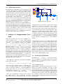
Example 1 shown in Figure 1. The presented hydraulic
system contains a heater, a three-way valve and a pump
setting the mass flow rate. The pump is connected to
nRes.k parallel pressure drop components res. The only
two states are the temperatures of the heater and the
pump with a time constant of 10 and 1 seconds, respectively. A pulsed signal sets the mass flow rate of
the pump and the outlet temperature of the heater. The
valve opening is set to 50%. The results are generated
for nRes.k = 20 unless stated otherwise.
For the given configuration Dymola generates the
following algebraic loops:
Sizes nonlinear systems of equations
Sizes after manipulation
{6,
{1,
21,
19,
46}
22}
Based on the C-code generated by OpenModelica, the
following algebraic loops are generated:
Sizes nonlinear systems of equations
Sizes after manipulation
{7,
{1,
41,
20,
47}
23}
In Dymola, these algebraic loops can be analysed using the dsmodel.mof file. The first system solves for
the mass flow rate in the left part of the fluid loop. The
second system solves for the mass flow rate in the right
part of the fluid loop. The third system solves for the enthalpies of the components in the right part of the fluid
loop.
Dymola’s BlockTimers generate the following output
for the system dynamics:
Name of block,
Block, CPU[s],
DynamicsSection:
14, 0.200, ...
Dynamics 2 eq:
15, 0.000, ...
Dynamics code:
16, 0.000, ...
Nonlin sys(1):
17, 0.007, ...
Dynamics code:
18, 0.000, ...
Dynamics 20 eq:
19, 0.066, ...
Dynamics code:
20, 0.002, ...
Nonlin sys(22):
21, 0.122, ...
Dynamics code:
22, 0.001, ...
heatCapacitor
C
cos
K
62
thermalConductor
thermalConductor1
G=1
G=1
freqHz=100
K
T=273.15
Figure 2. Example generating linear system of 2 equations
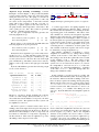
A common approach for decoupling algebraic loops
is adding additional states (Zimmer, 2013). However,
this can introduce fast dynamics, necessitating short time
steps during parts of the simulation. The values of the
state variables are solved by the integration algorithm,
and hence they reduce the size of the algebraic loops. A
simple example is shown in Figure 2 where a system of
two linear equations is generated when the heat capacitor
is unconnected. This system is decoupled when a heat
capacitor is added, since the temperatures at the ports
connecting the two conductances are then equal to the
state variable of this heat capacitor and need no longer
be obtained by solving an algebraic loop.
The enthalpy calculation of Example 1 can be
simplified in a similar way by adding nRes.k mixing
volumes at the location of the blue dot in Figure 1,
introducing a state in the flow path with a time constant
for the enthalpy of 10 s. The state values for the
enthalpy cause the system to become decoupled. The
system size is now reduced from 46/47 to 4/7 before
the manipulation, and from 22/23 to 1/3 after the
manipulation for Dymola/OpenModelica, regardless
of the value of nRes.k. Note that adding states also
changes the simulation results.
In this example, a second approach is possible. We
know that the fluid will always flow from the pump into
the resistance. Therefore the inflow enthalpy of the resistances is always equal to the enthalpy leaving the pump.
This knowledge can be passed on to the model by setting
allowFlowReversal=false in the components where
no flow reversal occurs. This causes the min and max attributes of the m_flow variable of the fluid ports to be
set to zero. Dymola utilizes this and simplifies equations
such as
Blocks 17, 19 and 21 clearly dominate the computa- H_out
tional cost of this example. The Dymola file dsmodel.c
shows that these block numbers correspond to the three
into
non-linear systems. We explain how these systems can
H_out
be simplified or removed.
or
The third system is created because there are no
enthalpy states in the right circuit except in the pump. In
general, the fluid can flow in both directions. Therefore
the inlet and outlet enthalpies of all res components can
be a function of all other res components, depending on
the flow direction. This causes an algebraic loop since
all enthalpy values depend on each other.
fixedTemperature
prescribedTemperature
= semiLinear(port_a.m_flow,
inStream(port_a.h_outflow),
port_a.h_outflow)
= port_a.m_flow * inStream(port_a.h_outflow)
H_out = port_a.m_flow * port_a.h_outflow .
It can conduct this simplification because the solver can
now take into account that the mass flow rate will never
become negative (or positive). Due to the simplified
structure of the problem, the solver is able to sort the
enthalpy equations in such a way that no algebraic loop
is formed: the solver can evaluate the equations sequentially, following the fluid downstream starting from
Proceedings of the 11th International Modelica Conference
September 21-23, 2015, Versailles, France
DOI
10.3384/ecp1511859
Session 2B: Building Energy Applications 1
N: Initial model
N: Enthalpy state
N: No flow reversal
A: Enthalpy state
A: No flow reversal
Succesful
steps
55
54
55
54
55
Jacobian
evaluations
21
20
21
20
20
Function
evaluations n f g
647
1448
647
547
557
Continuous
time states
2
22
2
22
2
Mean time
dynamics sec. [µs]
310
103
109
137
116
Total time
dynamics sec. [s]
0.200
0.150
0.071
0.075
0.065
Table 1. Solver output for 3 configurations of Example 1 (Figure 1), with nRes.k = 20 and analytic (A) or numeric (N) Jacobian
1.0
initial model
enthalpy state
allowFlowReversal = False
0.6
CPUtime [s]
CPUtime [s]
1.0
0.8
0.4
0.2
0.0
5
10
15
20
nRes.k
25
30
35
(a) numeric Jacobian
initial model
enthalpy state
allowFlowReversal = False
0.8
0.6
0.4
0.2
0.0
5
10
15
20
nRes.k
25
30
35
(b) analytic Jacobian
Figure 3. Simulation time for three variants of Example 1
known values of state variables. This causes the equations to be solved explicitly. OpenModelica does not
make this simplification and consequently the algebraic
loop size remains unchanged.
A different approach can be taken to break algebraic
loops without relying on the solver to make simplifications. Many fluid components contain equations such as
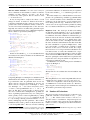
function evaluations that is required: 647 instead of
1448. The increased number of function evaluations is
caused by the increased number of states in the model. It
turns out that the higher number of state variables leads
to significantly more function evaluations, probably because by default, Dymola computes a numerical approximation to the Jacobian based on numeric differentiation.
port_a.h_outflow = inStream(port_b.h_outflow);
port_b.h_outflow = inStream(port_a.h_outflow);
Due to the performance penalty for approximating
the Jacobian, the simulations are repeated using an analytic Jacobian, which can be done in Dymola by setting
Advanced.GenerateAnalyticJacobian=true. In
OpenModelica, an option for this exists in the simulation setup. Results are shown in Figure 3b and in Table 1. The penalty for adding new states is almost completely removed when using an analytic Jacobian. Somehow the average execution time for the dynamics section increased slightly, even though the equations did not
change. The reason for this is unclear. The results indicate that the analytic Jacobians should be used whenever
possible, especially for models with a large amount of
states.
which may be simplified into
port_a.h_outflow = if allowFlowReversal
then inStream(port_b.h_outflow)
else Medium.h_default;
port_b.h_outflow = inStream(port_a.h_outflow);
because the value of port_a.h_outflow should
never be required for calculations upstream of port_a.
Therefore it does not matter what its value is. Choosing
a fixed value has the advantage that it allows breaking
algebraic loops. Note that when the flow does reverse,
the model equations will be wrong, which may cause
unstable dynamics.
Figure 3a shows the influence of these two measures
on the simulation time. Adding enthalpy states only reduced the computing time for nRes.k>20. However,
setting allowFlowReversal=false led to faster simulations. Note that the speed increase for the first case
depends on the time constants of the new states. Larger
time constants in general lead to faster simulations, but
may introduce non-physical dynamics.
The first three rows of Table 1 allow analysing the results in further detail. Both measures allow reducing the
computational work for each evaluation of f and g in
the dynamics section from 310 µs to ∼ 106 µs.
The overall speed when using allowFlowReversal=
false is however better due to the lower number of
DOI
10.3384/ecp1511859
From this analysis we conclude that the user
should be cautious when adding states for decoupling algebraic loops.
If they are added, setting
Advanced.GenerateAnalyticJacobian=true may
reduce computing time. An alternative approach is to use
physical insight to simplify the equations where possible, in a way similar to setting allowFlowReversal=
false. Also, it may be beneficial to remove the
states that are added by default in three-way valves and
other components containing mixing volumes. This can
be done by setting energyDynamics=massDynamics=
SteadyState. Most likely this change will create larger
systems, but often these can be simplified using the approach explained above.
Proceedings of the 11th International Modelica Conference
September 21-23, 2015, Versailles, France
63
Simulation Speed Analysis and Improvements of Modelica Models for Building Energy Simulation
from_dp = False
from_dp = True
0.20
0.15
CPUtime [s]
CPUtime [s]
0.25
0.10
0.05
0.00
5
10
15
20
nRes.k
25
30
35
Figure 4. Example 1 illustrating computation time for solving
mass flow rates through parallel resistances
6
5
4
3
2
1
0
from_dp = false
from_dp = true
2
4
6
8
nRes.k
10
12
14
Figure 5. Example 2 illustrating computation time for solving
mass flow rates through resistances in series
phiSat
Tin
phi
Algebraic Loops Iterating on Mass Flow Rates
and Pressures When setting allowFlowReversal=
false, the remaining computation time is almost entirely used for computing the mass flow rates and pressures. We now focus on reducing this computing time
further.
The pressure drop equations in this non-linear system
can be written either as ṁ = f (∆p) or as ∆p = f −1 (ṁ) for
some function f (·) or its inverse f −1 (·). The value of the
parameter res.from_dp will pick one or the other formulation. If from_dp=false, then the system has size
21/22 before and 19/20 after manipulation, otherwise it
has sizes 21/22 and 1/1 in Dymola/OpenModelica. This
can be explained as follows. When from_dp=true, the
mass flow rate is calculated as a function of the pressure
difference ∆p. Therefore ∆p is chosen as an iteration
variable. The symbolic processing algorithm detects that
all resistances are in parallel and hence must have the
same pressure drop. Therefore, they can all use the same
iteration variable, leading to a much smaller system. This
leads to a significant speed improvement, as shown in
Figure 4.
Example 1 uses a pump which sets the mass flow rate
to an input value and which is connected to nRes.k parallel pressure drop components. The solver can exploit
the system structure by selecting the common pressure
drop as an iteration variable. The “dual” problem (Example 2) could be to consider a pump which takes the
pressure drop as an input value and which is connected to
nRes.k pressure drop components connected in series.
In this case, it is advantageous to set from_dp=false
since Dymola and OpenModelica then select the common mass flow rate as the iteration variable, as illustrated
in Figure 5.
These were fairly simple problems. In practice, combinations of parallel and series connections are used,
making the choice of the parameter from_dp difficult.
However, it is often possible to aggregate multiple pressure drop components that are connected in series. If
all components have the same nominal mass flow rate
m_flow_nominal, then the nominal pressure drops dp_
nominal can be added into one component, reducing
the series branch into a single pressure drop equation.
Otherwise dp_nominal needs to be rescaled. This ap64
T
k=1
duration=1
m_condens
mCond
X_steam
vol
T
V=1
xSat
sink
bou
eps=0.8
T
senTem
m
res
hex
Figure 7. Example 4 illustration
proach can also be used when a valve is connected in
series to the pressure drop components. The valve parameter dpFixed_nominal should then be used.
Figure 6a shows Example 3 where nRes.k parallel instances of a series connection of two resistances
are simulated. The simulation time for this example is
shown in Figure 6b. The parameter mergeDp indicates
whether the two resistances are merged into one. Merging the two resistances gives much better results, especially when combined with from_dp=true. However
when the two resistances are not merged, it is better to
set from_dp=false.
Model Design for Avoiding Algebraic Loops Developers should avoid coupling systems of equations that
are only weakly dependent. Consider for instance the
model of a condensing heat exchanger. Such a model
contains equations for the pressure drop, heat flow rate
and water vapour condensation. One should try to avoid
coupling these equations into one algebraic loop.
Example 4 in Figure 7 shows a simple condensing heat
exchanger model. Along the flow path, first air cools
in the heat exchanger hex, then condensate is extracted
from the stream in vol (steady state) and finally the remaining mass is sent through a pressure drop component.
Ideally the solver would be able to first compute the mass
flow rate based on the pressure drop characteristic. Using
this mass flow rate, the heat flow rate can be computed
since it only depends on inlet temperatures and mass flow
rates. Finally moisture can be extracted such that the air
stream becomes saturated. In practice this sequential calculation is not possible because removing water vapour
from the air affects its mass flow rate and therefore also
the pressure drop. As a consequence the equations for the
Proceedings of the 11th International Modelica Conference
September 21-23, 2015, Versailles, France
DOI
10.3384/ecp1511859
Session 2B: Building Energy Applications 1
pulse
10
mergeDp = true, from_dp = false
mergeDp = false, from_dp = false
mergeDp = true, from_dp = true
mergeDp = false, from_dp = true
8
bou
CPUtime [s]
m_flow_in
P
m_flow
period=1
pump
mergeDp
res
from_dp
res1
nRes
6
4
2
0
true
true
2
4
6
8
nRes.k
10
12
14
k=6
(b)
(a)
Figure 6. Example 3 (a) illustration for solving mass flow rates through parallel instancs of a series connection of two resistances
and (b) simulation time based on two parameters (mergeDp and from_dp)
mass flow rate, heat flow rate and moisture balance are
coupled into a single system of 12/10 non-linear equations before manipulation in Dymola/OpenModelica.
As a simplification one could argue that the impact of
the water vapour mass flow rate on the pressure drop is
very small and that it could therefore be removed from
the mass conservation equation ∑ ṁ = 0. This physical approximation decouples the algebraic loop so that
in both simulation tools the equations can be solved sequentially.
We conclude from this discussion that the developer
should consider to approximate equations if such
approximations allow decoupling large systems of
equations while maintaining the accuracy required by
the application.
In some cases analytical solutions to nonlinear system of equations may exist. Especially linear system
of equations can often be solved analytically. To enable this, the solver needs to be able to establish whether
a system is linear. When using a Modelica function
in a system of equations, it is therefore important that
annotation(Inline=true) is used. When using this
annotation, the model developer suggests to the symbolic
processor to substitute the function call with the body
of the Modelica function, thereby allowing the symbolic
processor to detect the linearity. This allows symbolic
manipulation, such that algebraic loops can be simplified.
Setting in Dymola the option Evaluate=true may
also cause analytical solutions to be found, especially for
linear algebraic loops. However, this leads to parameter
values to be evaluated during translation, and hence they
can no longer be changed without translating the model
again.
3.1.2
Overhead Due to Inefficient Code
In general, every implemented equation will be evaluated. Simulation tools are able to perform certain code
simplifications such as common subexpression evaluation and detection of alias variables, but the level of optimization is not exhaustive. Therefore the developer
should be aware of how the solver treats equations. Here
we illustrate some important aspects.
Inlining functions Inlining functions may allow better symbolic processing. It can also lower the function evaluation time, probably because overhead for calling a C-function is avoided. We recommend to set
Inline=true by default for all functions, unless their
body is large.
Model Parameters
code listing below:
Consider Example 5 shown in the
model Example5
parameter Boolean efficient = false;
parameter Real[3] a = 1:3;
parameter Real b = sum(a);
Real c;
equation
der(c) = sin(time)*
(if efficient then b else sum(a));
end Example5;
The corresponding code in dsmodel.c is
helpvar[0] = sin(Time);
F_[0] = helpvar[0]*(IF DP_[0] THEN W_[0]
ELSE DP_[1]+DP_[2]+DP_[3]);
adding annotation(Evaluate=true) to the definition of efficient results in
helpvar[0] = sin(Time);
F_[0] = helpvar[0]*(DP_[0]+DP_[1]+DP_[2]);
This can be further improved by setting efficient=
true
These examples illustrate that even using existing helpvar[0] = sin(Time);
component models can be a challenge. Ideally this level F_[0] = helpvar[0]*W_[1];
of complexity is not exposed to the end user. A possi- The new code contains less operations, even though the
ble approach to do this is to construct often used base implementation is mathematically identical. Taking this
into account allows implementing more efficient models.
circuits that are preconfigured in an efficient way.
DOI
10.3384/ecp1511859
Proceedings of the 11th International Modelica Conference
September 21-23, 2015, Versailles, France
65
Simulation Speed Analysis and Improvements of Modelica Models for Building Energy Simulation
Obsolete Model Variables In some cases it may be
wise to eliminate model variables. Consider for instance
variables a, b and c where b = 2a and c = 2b. If b is
not used in any other equation, then it is better to write
c = 4a and remove b.
It may be important to analyse the effects of such
changes in detail. Consider for instance the model of
a discretised wall. The model consists of a series of temperature states with an adiabatic boundary condition on
one side and a sinusoidal temperature on the other side.
Typically, this will be modelled using thermal capacitances C and thermal resistors R. A Modelica implementation could be as presented by Example 6.
performance difference is unclear but may be explained
by the extra variables Q_flow, which may generate overhead.
From this analysis we conclude that there exists unexploited code optimization potential in popular Modelica
tools. Certain variables can be eliminated and dummy
parameters can be introduced to avoid parameter divisions during each time step. Until these issues are resolved, users can avoid performance penalties by taking
into account these limitations by reformulating models.
Real[nTem] T;
equation
der(T[1]) = ((273.15+sin(time))-2*T[1]+T[2])
*tauInv;
for i in 2:nTem-1 loop
der(T[i]) = (T[i-1]-2*T[i]+T[i+1])*tauInv;
end for;
der(T[nTem]) = (T[nTem-1]-T[nTem])*tauInv;
end Example7;
model Example8
Real a = sin(time+1);
Real b = sin(time+1);
end Example8;
Duplicate Code The developer should avoid making
models that generate duplicate code. A good example is
model Example6
a window model, which requires the solar irradiance to
parameter Integer nTem = 500;
be calculated. Since this calculation is influenced by paparameter Real R = 0.001;
rameters such as the window orientation and inclination
parameter Real C = 1000;
Real[nTem] T;
angle, the developer may choose to include these equaReal[nTem+1] Q_flow;
tions in the window model. If multiple windows have
equation
Q_flow[1] = ((273.15+sin(time))-T[1])/R;
the same orientation and inclination, then this means that
der(T[1]) = (Q_flow[1]-Q_flow[2])/C;
the same calculation is repeated multiple times. This
for i in 2:nTem loop
is not necessarily a problem if the overhead is small.
Q_flow[i] = (T[i-1] - T[i])/R;
der(T[i]) = (Q_flow[i]-Q_flow[i+1])/C;
However, in the case of a window model, the compuend for;
tation involves a lot of trigonometrical calculations and
Q_flow[nTem+1] = 0;
it would be better to isolate this calculation in a sepaend Example6;
In this model variables Q_flow are calculated but not rate model. An example implementation of this problem
necessarily needed. These variables can be eliminated as can be found in the IDEAS library (Baetens et al., 2015).
However, putting the solar irradiation in a separate model
illustrated in Example 7.
requires the user to keep the radiation computation conmodel Example7
sistent among multiple models.
parameter Integer nTem = 500;
parameter Real R = 0.001;
An illustration of common subexpression elimination
parameter Real C = 1000;
is
given
by Example 8.
parameter Real tauInv = 1/(R*C);
Comparing Example 7 to Example 6 a variable has been
eliminated but the number of operations within the for
loop remains the same. In particular, there are two additions and two divisions in Example 6, and two additions and two multiplications in Example 7. However, Example 7 is ∼ 83% faster in Dymola (2.83 s
→ 0.49 s) and OpenModelica (9.2 s → 1.6 s). It
turns out that this is mostly because a division generates more overhead than a multiplication, probably because of guarding against division by zero. This performance penalty can be reduced significantly by adding
annotation(Evaluate=true) to parameters R and
C, or by creating a dummy parameter similar to tauInv
and by multiplying with this parameter. This reduces
simulation time to 0.65 s > 0.49 s in Dymola and 2.39 s
> 1.6 s in OpenModelica.1 The reason for the remaining
1 These CPU times are based on the total Dynamics section time
in Dymola and the ‘simulation’ timer in the Statistics output of Open-
66
The Dymola C-code evaluates the sine and addition only
once:
W_[0] = sin(Time+1);
W_[1] = W_[0];
This simplification is not made in OpenModelica since it
evaluates the sin(·) function once for a and once for b.
Still, more complicated common subexpressions such
as in IDEAS are not detected by both tools. Therefore,
improving the common subexpression elimination would
allow further performance improvements.
3.2 Number of Evaluations
The previous section focussed on how to reduce the computational overhead for each evaluation of f (·, ·, ·, ·) and
g(·, ·, ·, ·). The current section focusses on how to reduce the number of evaluations. Important aspects are
the time constants of the system, the system stability, the
number of events, computing the Jacobian and the integrator choice.
Modelica when performing 100 000 Euler integration steps of Example 6 and Example 7.
Proceedings of the 11th International Modelica Conference
September 21-23, 2015, Versailles, France
DOI
10.3384/ecp1511859
Session 2B: Building Energy Applications 1
System Time Constants When a system has fast dynamics, then the solver has to track these dynamics with
small step sizes. In general, systems with large time constants have shorter calculation times. It may therefore
be advantageous to make certain dynamics slower, especially the fastest dynamics in the system. Dymola option
“Which states that dominate error” may be used to identify these states. Changing the dynamics may however be
non-physical or introduce instability in feedback control
loops. In this case a different option may be to remove
the fast dynamics completely and simulate the system as
a steady state system. Note, however, that this may increase the size of the algebraic system of equations.
The latter approach may be very effective when
considering air flow networks. If air is modelled
as compressible, pressure states are created in instances of MixingVolume, unless massDynamics=
SteadyState. These states however introduce small
time constants if part of a building air flow network. It
may therefore be better to remove them. Again, this may
create larger systems of equations.
System Stability If a feedback control loop is tuned
badly, oscillatory behaviour can occur. A variable time
step integrator may track these oscillations, leading to a
major decrease in simulation speed. Note that it may be
difficult to see these oscillations when the output interval
is set too large.
Number of Events Events require the integration to
stop and restart, typically with a lower order method and
with smaller time steps. In addition, for state events, typical ODE solvers require an iterative solution to find the
time when the event happens.
Computing the Jacobian Some integrators require the
Jacobian to be calculated. Having more states leads to a
larger Jacobian, as was illustrated in Example 1. Since
by default, Dymola and OpenModelica use numeric differentiation to approximate the Jacobian, a lot of finite
differences need to be calculated, each requiring a function evaluation. Note that in particular models with a
larger number of states benefit more from having an analytic Jacobian, since the number of Jacobian entries
equals the square of the number of states.
Integrator Choice Many integrators use an implicit
integration scheme. This typically requires the computation of a Jacobian and requires iterations to be performed before reaching convergence. This can lead to
more function evaluations. However, for stiff systems,
implicit integrators are more efficient than explicit integrators.
DOI
10.3384/ecp1511859
3.3 Analysis of Large Problems
In the previous sections, computing time was analysed
using small models. In building simulation, models can
however become considerably larger and analysing the
computational speed can be difficult since it depends on
a lot of factors, including the unknown solver implementation. Still, we predict some trends for the computation
time, based on the size of the model.
Consider a model of a district energy system, including building models and an electrical grid. When doubling the size of the district, ideally the computational
time would double as well, such that computational time
scales linearly with problem size. Let us analyse this
further based on Equation 12. Ideally t f g scales linearly
with the problem size. In practice this is not necessarily the case. The electrical grid of the district typically
results in a large non-linear system of equations since
all electrical components have very fast transients and
are therefore modelled as steady state components. Doubling the size of the model therefore also doubles the size
of the algebraic loop. Example 1 has shown that computational time for algebraic loops does not scale linearly
with size and therefore larger models will become computationally slow. Equations outside algebraic loops can
be solved sequentially. Therefore their computational
time does scale linearly.
Because t f g scales, at best, linearly with size, n f g
should remain constant if we want to obtain overall linear scaling of the computational time. However, firstly,
generally n f g also grows with problem size, for example
because larger problems have more controllers that may
trigger events. If the amount of buildings doubles, then
the amount of state events may double, which causes a
performance penalty. Secondly, when a numeric Jacobian needs to be computed, then n f g will increase since
the number of states increases linearly with the problem size. The number of operations for an implicit integrator typically does not scale linearly either. Solving
dense implicit systems typically requires O(n3 ) operations (Hairer and Wanner, 2002). Building model Jacobians are however very sparse. It is not clear how
well this is exploited by Dymola. An integrator such as
Rkfix4 can have an operation count that is linear with
the problem size, unless the fixed time step is changed.
For certain large problems that do not require event handling, it can therefore be advantageous to use these simple integrators, also because they do not require a Jacobian to be calculated.
3.3.1
Parallelization
Dymola supports parallelization for the calculation of f (·, ·, ·, ·) and g(·, ·, ·, ·) (Dassault
Systèmes, 2014) and analytic Jacobian (see
Advanced.ParallelizeAnalyticJacobian).
However parallelization generates overhead for syn-
Proceedings of the 11th International Modelica Conference
September 21-23, 2015, Versailles, France
67
Simulation Speed Analysis and Improvements of Modelica Models for Building Energy Simulation
Integrator
Dassl
Dassl
Radau IIa
Lsodar
Lsodar
Lsodar
Dopri45
Dopri45
Rkfix4
Rkfix4
Rkfix4
Euler
Euler
Tolerance
/ step size
1 E-6
1 E-4
1 E-6
1 E-6
1 E-4
1 E-2
1 E-6
1 E-8
20 s
5s
1s
5s
0.25 s
CPUtime
[s]
4261
3088
4042
3450
2073
1655
194
199
15.4
50.6
224
24.0
446
Dynamics
section [s]
3538
2759
2400
2666
1435
1152
159
162
11.3
42.9
202
18.2
389
Outside of
model [s]
476
327
1416
547
515
406
17.0
18.3
1.1
1.5
3.2
1.7
12.8
Function
evaluations n f g
787341
546326
453073
679486
347018
256458
41166
42017
2717
10233
50211
4271
80233
State
events
41
36
37
44
41
38
39
39
39
43
38
50
41
Time
events
8
8
8
8
8
8
8
8
8
8
8
8
8
Jacobian
evaluations
1235
862
347
1047
537
399
0
0
NA
NA
NA
NA
NA
Eel
[error]
-4.35 E-6
3.17 E-3
1.64 E-3
-4.35 E-6
-2.25 E-5
4.51 E-3
4.68 E-4
1.96 E-6
1.34 E-2
2.52 E-3
1.28 E-3
-2.00 E-3
-4.22 E-4
Table 2. Example building model statistics for various integrators and tolerance options. Results are the solution statistics (when
available, else ‘NA’) and the relative error of Eel
3.3.2
Example of Large Building Model
The approach explained in this paper was applied to a
building model based on a real case (Solarwind, Luxemburg), containing 32 IDEAS (Baetens et al., 2015)
building zones with individual concrete core activation
circuits (Baetens et al., 2015) and Variable Air Volume (VAV) boxes including heating battery, bore field
model (Picard and Helsen, 2014), solar collector (Wetter et al., 2014), four thermal storage devices (Wetter
et al., 2014), one pellet boiler, four heat pumps (Baetens
et al., 2015), two adiabatic/active heat recuperating air
handling units, pumps (Wetter, 2013) and valves (Wetter et al., 2015) and a control strategy based mostly on
hysteresis controllers, PID controllers, heating/cooling
curves and boolean algebra. The model has 2468 continuous time states and 28342 time-varying variables.
Special care was taken to make sure that the smallest time constants are in the order of 30 s. Therefore air
ducts are steady state, pumps and valves have no opening delay or filter and pipes were lumped into only a few
states per circuit branch, thereby allowing to increase
the time constant. Temperature sensors are assumed to
have a time constant in the order of one minute. Using
dynamic sensors avoids coupling the thermal equations
with the control equations into a single algebraic loop.
This model was simulated for tend − tstart = 10 000 s
using various implicit integrators, with numeric Jacobians and explicit integrator Dopri45. The total amount
of function evaluations exceeds 40 000 in each case. This
is on average one function evaluation every 0.25 s, while
the smallest time constant of the system is ∼ 30 s. Therefore it makes sense to use an explicit fixed step integrator. Table 2 shows the results, including fixed step ex68
104
CPUtime [s]
chronization and communication. The authors have not
been able to gain notable improvements in simulation
speed in building applications by using parallelization in
Dymola 2015 FD01.
Euler
Rkfix4
Dopri45
dassl
Lsodar
Radau
103
102
101 -6
10
10-5
10-4
10-3
10-2
Relative error Eel
10-1
100
101
Figure 8. Relative errors of Eel for various solvers and tolerances or fixed time step sizes
plicit integrators Rkfix4 and Euler. It contains statistics and the error on one simulation result that is of interest, namely the integrated electrical power consumption
of the building Eel . The relative error was calculated using Dassl with a tolerance of 10−8 , which produced a
result of 4.591880 kWh.
From these results and Figure 8 it is clear that implicit
integrators are very slow compared to explicit integrators
for this problem. Fixed step methods are especially fast
when high accuracy is not required, allowing a simulation speed 500 times faster than real time, which is more
than 100 times faster than Dassl. For higher accuracies,
Dopri45 can be used. Lsodar is the fastest implicit integrator that was tested. Note that the simulation can easily
be made faster by using a larger step size, at the cost of
accuracy. Also, using larger step sizes will eventually
lead to numerical instabilities. The user may therefore
want to adjust the dynamics of the system, or set certain
dynamics to steady state. It is thus important that models
expose these parameters and allow easy configuration.
The achieved speed increase is considerable. However, this still requires about 18 hours for a one-year simulation. As this is longer than typical building energy
simulations, we think that further research is desirable to
reduce the simulation time further.
Proceedings of the 11th International Modelica Conference
September 21-23, 2015, Versailles, France
DOI
10.3384/ecp1511859
Session 2B: Building Energy Applications 1
4 Conclusion
We conclude that the analysis of algebraic loops, the
optimization of Modelica code and the application of
physical insight can lead to significant simulation time
improvements. Analysis of the model time constants,
avoiding system instabilities, using analytic Jacobians
and proper integrator choice can also be important.
These modifications were applied to a large building
model where removal of all ‘fast’ dynamics allowed explicit integrators to perform well. Fixed step integrators can also be used if simulation results do not need
to be very accurate. Euler integration performs very
well in terms of computation time, allowing detailed office building simulations at a speed 500 times faster than
real time.
Further work can focus on analysing and changing the
problem structure in such a way that parallelization can
be used efficiently. It should also be investigated up to
which extent models can be made faster by changing the
model dynamics, which allows larger time steps to be
taken, without introducing too large errors. The proposed changes demonstrate that further symbolic processing in Dymola and OpenModelica is possible. We
also propose to use analytic Jacobians by default for all
Jacobian elements where an analytic Jacobian can be
computed.
5 Acknowledgements
Earl A. Coddington and Norman Levinson. Theory of ordinary
differential equations. McGraw-Hill Book Company, Inc.,
New York-Toronto-London, 1955.
Dassault Systèmes. Dymola user manual, vol. 1, 2014.
Ernst Hairer and Gerhard Wanner. Solving Ordinary Differential Equations II: Stiff and Differential-Algebraic Problems.
Springer-Verlag Berlin Heidelberg, 2002.
Alan C. Hindmarsh. Odepack, a systematized collection of
ode solvers. IMACS transactions on scientific computation,
1:55–64, 1983.
Linda R. Petzold. Description of dassl: a differential/algebraic
system solver. Technical report, Sandia National Labs., Livermore, CA (USA), 1982.
Linda R. Petzold. Automatic selection of methods for solving
stiff and nonstiff systems of ordinary differential equations.
SIAM journal on scientific and statistical computing, 4(1):
136–148, 1983.
Damien Picard and Lieve Helsen. Advanced Hybrid Model for
Borefield Heat Exchanger Performance Evaluation, an Implementation in Modelica. In 10th International Modelica
Conference 2014, pages 857–866, Lund, 2014.
Elijah Polak. Optimization, Algorithms and Consistent Approximations, volume 124 of Applied Mathematical Sciences. Springer Verlag, 1997.
Michael Tiller. Introduction to Physical Modeling with Modelica. Springer US, 2001.
Michael Wetter. Fan and pump model that has a unique solu-
tion for any pressure boundary condition and control signal.
The authors acknowledge the financial support by the
In Jean Jacques Roux and Monika Woloszyn, editors, Proc.
Agency for Innovation by Science and Technology in
of the 13-th IBPSA Conference, pages 3505–3512, 2013.
Flanders (IWT) for the PhD work of F. Jorissen (contract
URL http://simulationresearch.lbl.gov/
number 131012).
wetter/download/2013-IBPSA-Wetter.pdf.
This research was supported by the Assistant Secretary for Energy Efficiency and Renewable Energy, Of- Michael Wetter, Wangda Zuo, Thierry S. Nouidui, and Xiufeng
Pang. Modelica buildings library. Journal of Building Perfice of Building Technologies of the U.S. Department of
formance Simulation, 7(4):253–270, 2014.
Energy, under Contract No. DE-AC02-05CH11231.
This work emerged from the Annex 60 project, an
Michael Wetter, Marcus Fuchs, Pavel Grozman, Lieve Helsen,
international project conducted under the umbrella of
Filip Jorissen, Moritz Lauster, Dirk Müller, Christoph
the International Energy Agency (IEA) within the EnNytsch-Geusen, Damien Picard, Per Sahlin, and Matthis
ergy in Buildings and Communities (EBC) Programme.
Thorade. IEA EBC annex 60 modelica library - an interAnnex 60 will develop and demonstrate new generation
national collaboration to develop a free open-source model
library for buildings and community energy systems. In
computational tools for building and community energy
Building simulation 2015, submitted, Hyderabad, 2015.
systems based on Modelica, Functional Mockup Interface and BIM standards.
References
Ruben Baetens, Roel De Coninck, Filip Jorissen, Damien Picard, Lieve Helsen, and Dirk Saelens. Openideas - an open
framework for integrated district energy simulations. In
Building simulation 2015, submitted, Hyderabad, 2015.
Dirk Zimmer. Using Artificial States in Modeling Dynamic
Systems : Turning Malpractice into Good Practice. In Proceedings of the 5th International Workshop on EquationBased Object-Oriented Modeling Languages and Tools,
pages 77–85, 2013.
François E. Cellier and Ernesto Kofman. Continuous System
Simulation. Springer US, 2006.
DOI
10.3384/ecp1511859
Proceedings of the 11th International Modelica Conference
September 21-23, 2015, Versailles, France
69