Download DISSERTATION TITLE (ALL CAPS, Line 1)

STUDY OF WIND LOADS APPLIED TO ROOFTOP SOLAR PANELS
by
JENNIFER DAVIS HARRIS
B.S., University of Colorado Denver, 2006
A thesis submitted to the
Faculty of the Graduate School of the
University of Colorado in partial fulfillment
of the requirements for the degree of
Master of Science
Civil Engineering
2013
This thesis for the Master of Science degree by
Jennifer Davis Harris
has been approved for the
Civil Engineering Program
by
Frederick R. Rutz, Chair
Kevin L. Rens
Yail Jimmy Kim
July 12, 2013
ii
Jennifer Davis Harris (M.S., Civil Engineering)
Study of Wind Loads Applied to Rooftop Solar Panels
Thesis directed by Assistant Professor Frederick R. Rutz
ABSTRACT
The results from a full-scale faux solar panel installation research project for two
panels placed near the edge of a building with a flat roof on the University of Colorado
Denver campus are presented. The building and campus are located in downtown
Denver, CO adjacent to a special wind region. A faux solar panel test frame was
developed to measure the forces imposed on a full scale solar panel mounted on a flat
roof. The measured wind direction, velocity, and corresponding barometric pressure are
used to determine the resultant force due to the velocity pressure on the face of the panel.
The resultant force is derived from the force measured from strain gages connected to a
diagonal tension tie on the test frame. The force coefficient CF is determined from the
ratio of the resultant panel force determined from strain measurements and the force
determined from the velocity pressure. CF values so determined are presented within.
The form and content of this abstract are approved. I recommend its publication.
Approved: Frederick R. Rutz
iii
DEDICATION
I dedicate this work to my parents Richard and Susan Davis and my
husband, Michael Harris who have patiently waited for me to complete this journey.
iv
ACKNOWLEDGMENTS
In an effort to express the sincerest form of gratitude to the multitude of
individuals who assisted with this project, the author wishes to acknowledge the
following individuals. Dr. Frederick R. Rutz, my advisor, who has been instrumental in
the organization and implementation of this project. Your wisdom, encouragement, and
support have not gone unnoticed. Without your assistance both physically and
intellectually, this project would not be where it is today. To my co-researcher and
fellow graduate student, Erin Dowds, who has graciously allowed me to participate in
this research project, this was your brainchild and although, I have finished first, credit is
due to you. I will be there to help you continue this research and I am sincerely grateful
for all of your help designing, building and carrying sand bags and faux solar panels on
the roof of the PE building. Sincere thanks is offered to Drs. Kevin Rens and Jimmy
Kim, of the Civil Engineering Department at UCD, not only for being part of my
graduate committee but also for the financial assistance provided for the calibration and
repair of the data logger. Next, I would like to thank Tom Thuis, Jac Corless, Denny
Dunn and Eric Losty of the Electronic Calibration and Repair Lab at UCD for the many
hours and late nights spent calibrating strain transducers, fabricating steel components
and diagnosing and repairing glitches in the testing equipment. Each of you is asset to
UCD and certainly to this project. To the Auraria Higher Education Campus Facilities
Department, thank you for providing access and allowing us to conduct our research on
the Events Center Building and to Pete Hagan for the prompt support. To Mick Harris
and Andy Andolsek I would like to express the sincerest gratitude for your help
constructing the solar panels and carrying them to the roof of the PE building along with
v
many sand bags. My freshly injured back would also like to thank you. I would also like
to gratefully acknowledge my boss, Jim Harris, for his encouragement and financial
assistance to pursue this graduate degree and the financial assistance involved with the
attendance of two conferences in support of this project. Finally to the many individuals
to assisted in one way another with support, encouragement and advice regarding this
project including but not limited to, Dorothy Reed, David Banks, Kishor Mehta, Franklin
Lombardo, and Ted Stathopoulos.
vi
TABLE OF CONTENTS
Chapter
1.
Overview...................................................................................................................... 1
1.1 Introduction.................................................................................................................. 1
1.2 Goal.............................................................................................................................. 2
2.
History of Solar Energy ............................................................................................... 4
2.1 Introduction.................................................................................................................. 4
2.2 History of Solar Energy ............................................................................................... 4
2.3 Wind Behavior and ASCE7 ......................................................................................... 7
2.4 Wind Tunnel Studies ................................................................................................. 10
2.6 Conclusions................................................................................................................ 20
3.
Panel Design, Location and Installation .................................................................... 22
3.1 Description ................................................................................................................. 22
3.2 Wind Load ................................................................................................................. 24
3.3 Design Calculations ................................................................................................... 26
3.4 Faux Solar Panel Test frame ...................................................................................... 27
vii
3.5 Connection Details..................................................................................................... 29
3.6 Assembly and Installation.......................................................................................... 31
4.
Instrumentation .......................................................................................................... 33
4.1 Introduction................................................................................................................ 33
4.2 Data Logger ............................................................................................................... 33
4.3 Solar Panel ................................................................................................................. 34
4.4 Strain Transducers ..................................................................................................... 35
4.4.1
Strain Transducer Fabrication ............................................................................... 35
4.4.2
Strain Transducer Calibration ............................................................................... 36
4.4.3
Strain Transducer Installation ............................................................................... 40
4.5 Anemometers ............................................................................................................. 41
4.6 Wind Direction Sensor .............................................................................................. 42
4.7 Thermocouple ............................................................................................................ 43
4.8 Interval Timer ............................................................................................................ 44
4.9 Software ..................................................................................................................... 44
5.
Theory ........................................................................................................................ 45
viii
5.1 Introduction................................................................................................................ 45
5.2 Wind Interaction with the Panel ................................................................................ 45
5.3 Calculations ............................................................................................................... 47
6.
Results and Discussion .............................................................................................. 54
6.1 Introduction................................................................................................................ 54
6.2 Results........................................................................................................................ 54
6.3 Discussion .................................................................................................................. 85
7.
Summary, Conclusions, Possible Sources of Error and Recommendations for Future
Research ............................................................................................................................ 91
7.1 Summary .................................................................................................................... 91
7.2 Conclusions................................................................................................................ 91
7.3 Possible Sources of Error........................................................................................... 92
7.4 Recommendations for Future Research ..................................................................... 93
References ......................................................................................................................... 96
ix
Appendix
A. Campbell Scientific CR5000 Data Logger Information ............................................ 98
B. Creating a Program Using Short Cut ....................................................................... 102
C. Editing a Program Using CRBasic Editor ............................................................... 131
D. Program.................................................................................................................... 146
x
LIST OF TABLES
Table
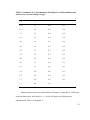
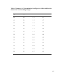
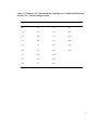
6.1 Summary of CF determinations from Figure 6.1 within wind direction tolerance for
3-second rolling averages ................................................................................................. 56
6.2 Summary of CF determinations from Figure 6.3 within wind direction tolerance for
9-second rolling averages ................................................................................................. 59
6.3 Summary of CF determinations from Figure 6.4 within wind direction tolerance for
3-second rolling averages ................................................................................................. 61
6.4 Summary of CF determinations from Figure 6.5 within wind direction tolerance for
3-second rolling averages ................................................................................................. 63
6.5 Summary of CF determinations from Figure 6.6 within wind direction tolerance for
3-second rolling averages ................................................................................................. 65
6.6 Summary of CF determinations from Figure 6.7 within wind direction tolerance for
3-second rolling averages ................................................................................................. 67
6.7 Summary of CF determinations from Figure 6.8 within wind direction tolerance for
3-second rolling averages ................................................................................................. 69
xi
6.8 Summary of CF determinations from Figure 6.9 within wind direction tolerance for
3-second rolling averages ................................................................................................. 71
6.9 Summary of CF determinations from Figure 6.10 within wind direction tolerance for
3-second rolling averages ................................................................................................. 73
6.10 Summary of CF determinations from Figure 6.11 within wind direction tolerance for
3-second rolling averages ................................................................................................. 75
6.11 Summary of CF determinations from Figure 6.12 within wind direction tolerance for
3-second rolling averages ................................................................................................. 76
6.12 Summary of CF determinations from Figure 6.13 within wind direction tolerance for
3-second rolling averages ................................................................................................. 78
6.13 Summary of CF determinations from Figure 6.14 within wind direction tolerance for
3-second rolling averages ................................................................................................. 80
6.14 Summary of CF determinations from Figure 6.15 within wind direction tolerance for
3-second rolling averages ................................................................................................. 82
6.15 Summary of CF determinations from Figure 6.16 within wind direction tolerance for
3-second rolling averages ................................................................................................. 84
xii
LIST OF FIGURES
Figure
2.1 Principles of Wind Flow against a Bluff Body ............................................................ 9
2.2 Smoke Visualization Used in the Boundary Layer Wind Tunnel.............................. 12
2.3 Solar Collector Mounted on a Building with a Flat Roof and a Parapet ................... 13
2.4 Design GCp Values Published by SEAOC, August 2012 ......................................... 18
2.5 Figure 29.9-1 from SEAOC Document ..................................................................... 19
3.1 Location of the Solar Panels on the Event Center Building ...................................... 23
3.2 Location of the Solar Panels on the Event Center Building ...................................... 23
3.3 Location of the Solar Panels on the Event Center Building ...................................... 24
3.4 Site Location of the University of Colorado Denver ................................................. 25
3.5 Panel A Construction Overview ................................................................................ 27
3.6 Panel B Construction Overview................................................................................. 28
3.7 Panel B Construction Overview................................................................................. 28
3.8 Panel Frame Connection Details.at the Diagonal Tension Ties ................................ 30
3.9 Panel Frame Connection Details in the Short Dimension ......................................... 30
xiii
3.10 Close-Up View of Short Direction Panel Frame Connection Details ...................... 31
3.11 Panel Layout and Location ...................................................................................... 32
4.1 Campbell Scientific CR5000 Data Logger ................................................................ 34
4.2 SP20 Solar Panel Used to Power the CR5000 Data Logger ...................................... 35
4.3 Strain Transducer ....................................................................................................... 36
4.4 Strain Transducer Calibration Set-Up ........................................................................ 37
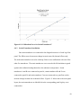
4.5 Calibration Curve for Strain Transducer A ................................................................ 37
4.6 Calibration Curve for Strain Transducer B ................................................................ 38
4.7 Calibration Curve for Strain Transducer C ................................................................ 38
4.8 Calibration Curve for Strain Transducer D ................................................................ 39
4.9 Calibration Curve for Strain Transducer E ................................................................ 39
4.10 Calibration Curve for Strain Transducer F .............................................................. 40
4.11 Strain Transducer Instrumentation Plan................................................................... 41
4.12 RM Young 3101 Anemometer................................................................................. 42
4.13 Overview of Anemometer and Vane Installation .................................................... 43
5.1 Schematic Diagram of Wind Interaction at Panel B .................................................. 46
xiv
5.2 Schematic Diagram of Wind Interaction with Panel A ............................................. 46
5.3 Schematic Diagram of Forces Acting on the Panel Surface and Frame .................... 47
5.4 Schematic Time History Diagram of Wind Velocity and Strain ............................... 50
5.5 Filtered Wind Direction for CF Calculation ............................................................... 52
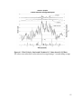
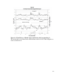
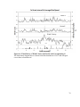
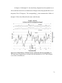
6.1 Wind Velocity, Strain and Calculated CF Values from 4/14/13 Data ....................... 55
6.2 Results of Wind Direction Plotted Versus CF from April 14, 2013 .......................... 57
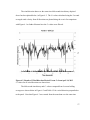
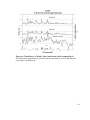
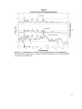
6.3 Wind Velocity, Strain and calculated CF Values from 4/14/13 Data ........................ 58
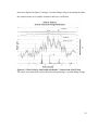
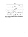
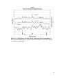
6.4 Time History of Wind Velocity and Strain with Corresponding CF.......................... 60
6.5 Time History of Wind Velocity and Strain with Corresponding CF.......................... 62
6.6 Time History of Wind Velocity and Strain with Corresponding CF.......................... 64
6.7 Time History of Wind Velocity and Strain with Corresponding CF.......................... 66
6.8 Time History of Wind Velocity and Strain with Corresponding CF.......................... 68
6.9 Time History of Wind Velocity and Strain with Corresponding CF.......................... 70
6.10 Time History of Wind Velocity and Strain with Corresponding CF........................ 72
6.11 Time History of Wind Velocity and Strain with Corresponding CF........................ 74
6.12 Time History of Wind Velocity and Strain with Corresponding CF........................ 76
xv
6.13 Time History of Wind Velocity and Strain with Corresponding CF........................ 77
6.14 Time History of Wind Velocity and Strain with Corresponding CF........................ 79
6.15 Time History of Wind Velocity and Strain with Corresponding CF........................ 81
6.16 Time History of Wind Velocity and Strain with Corresponding CF........................ 83
A.1 Campbell Scientific CR5000 Data Logger. .............................................................. 98
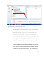
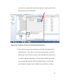
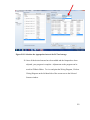
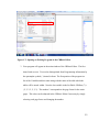
B.1 Procedure for Accessing Short Cut within RTDAQ Program ................................ 103
B.2 Creating a New Program in Short Cut .................................................................... 104
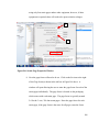
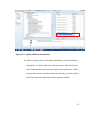
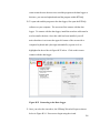
B.3 Selecting the Data Logger Model and Scan Interval in Short Cut .......................... 105
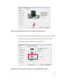
B.4 Available Sensors and Devices Menu in Short Cut ................................................ 106
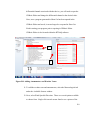
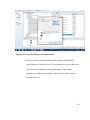
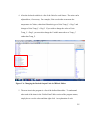
B.5 Adding a Strain Gage in Short Cut.......................................................................... 107
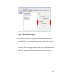
B.6 Strain Gage Properties Window .............................................................................. 108
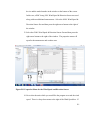
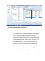
B.7 Setting the Gage Factor in the Properties Menu ..................................................... 109
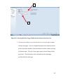
B.8 Adding Anemometers and Weather Vanes ............................................................. 110
B.9 Properties Menu for the Wind Speed and Direction Sensor ................................... 111
B.10 Setting the Units for the Wind Speed Measurements ........................................... 112
B.11 Adding additional Anemometers .......................................................................... 113
xvi
B.12 Properties Menu for the Anemometers ................................................................. 114
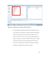
B.13 Example Error Message from Short Cut ............................................................... 115
B.14 Adding a Thermocouple ........................................................................................ 116
B.15 Thermocouple Properties Menu ............................................................................ 117
B.16 Selected Sensors Window ..................................................................................... 118
B.17 Selecting the Outputs for each Sensor................................................................... 119
B.18 Selecting the Outputs for each Sensor................................................................... 120
B.19 Selection the Appropriate interval for PCCard storage ......................................... 122
B.20 Accessing the Wiring Diagram ............................................................................. 123
B.21 Sample Wiring Diagram........................................................................................ 124
B.22 Saving the Program ............................................................................................... 125
B.23 Connecting to the Data Logger ............................................................................. 126
B.24 EZSetup Wizard for Connecting to the Data Logger ............................................ 127
B.25 Selecting the Data Logger for the Communication Setup..................................... 127
B.26 Selecting the Data Logger for the Communication Setup..................................... 128
B.27 Selecting the COM Port on your computer ........................................................... 129
xvii
B.28 Saving the Program ............................................................................................... 130
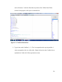
C.1 Accessing CRBasic Editor in the RTDAQ Program ............................................... 131
C.2 Accessing CRBasic Editor in the RTDAQ Program ............................................... 132
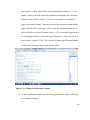
C.3 Opening an Existing Program in the CRBasic Editor ............................................. 133
C.4 Strain Gage factors .................................................................................................. 134
C.5 Adjusting the Strain Gage Factor in CRBasic Editor .............................................. 134
C.6 Changing the Desired Output Units in CRBasic Editor .......................................... 135
C.7 Data Tables and Editing the Data Interval in CRBasic Editor ................................ 136
C.8 Editing the Data Type ............................................................................................. 137
C.9 CardOut Instructions ............................................................................................... 138
C.10 CardOut Instructions ............................................................................................. 139
C.11 Editing the Differential Channel ........................................................................... 140
xviii
1.
Overview
1.1
Introduction
Overtime humankind has become dependent on electricity, the main source of
which is generated from fossil fuels. As time has passed and our knowledge has
increased, we have learned how the combustion of coal and other means of energy
production have contributed to negative impacts on our ecosystem. Because of this,
society has become increasingly interested in developing alternative methods of energy
production. Solar collectors have become a viable alternative source of energy for many
commercial and residential buildings. An attractive location for mounting solar panels is
on the roof of a structure. Typically, solar panels would be placed in a location and
orientation in which to maximize their exposure to the sun and thus collect the most solar
energy. Because of the placement of the panels on the roofs of buildings and on the
ground surface, the panels themselves are subjected to environmental phenomena such as
wind and snow loads. The interaction between the wind load, the solar panels, and
frames to which they are mounted produce significant forces on roof structure to which
they are attached. The design engineer must be consider these forces not only for the
design of the solar panels, but also for the frames to which they are mounted and the
connections between the frame and the roof structure. When solar panels are mounted on
the roofs of existing structures, the roof system must be checked to determine if it is
capable of resisting the uplift force applied to it by the solar panels. Engineering
standards typically used by design professionals, such as ASCE7 (ASCE7 2010), make
1
no mention as to what type of wind loads should be applied to roof mounted solar panels.
Because of this, the design professional is left to use his or her judgment to formulate an
appropriate methodology to determine design wind pressures on solar panels and their
effects on the roof structure.
1.2
Goal
The goal of this research is to determine the force coefficients acting on the face
of solar collectors mounted near the edge of a flat roof structure in order to calculate the
appropriate wind pressure for design. It is expected that the peak force coefficients
determined from this study will be well in excess of the pressure coefficients used in the
ASCE7 standard. However, the ASCE7 standard does not address the design of solar
panels. The results are offered for comparison with previous wind tunnel studies. The
proposed research was presented at the 3rd American Association of Wind Engineers
Workshop in Hyannis, MA, Aug. 12-14, 2012 (Dowds et al. 2012). In order to
accomplish this goal, two faux solar panel test frames were developed to measure the
resultant forces acting on the face of the solar panels. From these measurements force
coefficients were derived. The results of this study were presented at the 12th Americas
Conference on Wind Engineering in Seattle, WA, June 16-20, 2013 (Harris et al. 2013).
1.3
Outline
There are seven chapters in this thesis. The first chapter provides an overview and
includes a description of the goal of this research.
Chapter 2 is a literature review of the history of solar energy and a brief overview
of wind interaction on a bluff body. The standard used to determine wind pressures is
2
discussed as well as a summary of several wind tunnel studies which have been
previously conducted.
In Chapter 3, the design, location, and installation of the faux solar panel test
frames are discussed.
Chapter 4 is a summary of the instrumentation and equipment used to conduct this
research
In Chapter 5, the theory and methodology established to determine the appropriate
force coefficients is explained
Chapter 6 presents the results of this research from three different wind directions
and a discussion of the findings is presented.
Chapter 7 presents a summary of the results of this study and offers conclusions
based on these results. A discussion of possible sources of error is made and also
presented are recommendations for future research.
Appendix A provides some basic instructions regarding the usage of the CR5000
data logger.
In Appendix B, a brief instruction on how the program used for this research was
created using the Short Cut software provided with the data logger.
In Appendix C, a summary of instructions is provided in order to edit a program
which was created using the Short Cut software.
The program used for the purposes of this study has been provided in Appendix
D.
3
2.
History of Solar Energy
2.1
Introduction
The use of solar collectors as an alternative means of energy production is
becoming a viable alternative among many energy conscious businesses and
homeowners. The since the 1950’s when the silicon photovoltaic (PV) cells were
developed, efforts have been focused on increasing the efficiency of PV systems and
reducing their costs. With the decrease in cost, there has been an increase in solar
collector installations. Design professionals have little guidance for determining design
wind pressures acting on the solar panels. There is little agreement between the force
coefficients determined from previous wind tunnel studies. Full scale testing is necessary
to validate the results from these previous wind tunnel studies. The following chapter is a
literature review offering a brief summary of the history of solar energy, the basic
principles of bluff body aerodynamics and an overview of the results of some previous
wind tunnel studies.
2.2
History of Solar Energy
According to the U.S. Department of Energy, the earliest documented uses of
concentrating the sun’s energy date back to the 7th Century B.C, when magnifying glasses
were used to start fire (History of Solar 2012). It is documented that in 212 B.C.,
Archimedes used the reflective properties of bronze shields to concentrate the suns
energy and burn wooden ships from the Roman Empire while attacking the city of
Syracuse. By the 6th Century A.D. sunrooms were a common feature in most buildings
4
and the “Justinian code initiated sun rights to ensure individual access to the sun. (History
of Solar 2012). Around 1200 A.D. the Anasazi people built their homes in south facing
cliff dwellings in what is now referred to as Mesa Verde. In 1767 the first solar collector
was developed Horace de Saussure from Switzerland. The solar collector, perhaps more
appropriately labeled a “hot box” was constructed of five glass boxes stacked inside of
one another. The outermost box was twelve inches square and six inches high. The
innermost box was four inches square and two inches high (Hot Boxes 2012). In the
1860’s, Frenchmen, August Mouchet and Abel Pifre developed the first solar powered
engine which “became the predecessors of modern parabolic dish collectors.” Next, in
1891, the first solar powered water heater was developed in Baltimore by on Clarence
Kemp. By 1954, “photovoltaic technology was born in the United States” (History of
Solar 2012).
Daryl Chapin, Calvin Fuller, and Gerald Pearson of Bell Labs were the
scientists credited with developing the first, silicon photovoltaic cell which could convert
the sun’s energy to power and generate electricity. The photovoltaic cell was created
from a piece of silicon which contained a trace amount of gallium and lithium and was
approximately five times as efficient as the selenium solar cells used at the time (Perlin
2004). Over the next several decades many technological advances were made to
increase the efficiency of photovoltaic cells. By the mid 1960’s NASA created solar
powered space crafts and observatories. The world’s first solar powered residence was
constructed in 1973 by the University of Delaware. Named, “Solar One,” the residence
employed the use of a roof top solar array to provide power to the residence throughout
the daytime (History of Solar 2012). Between 1997 and 2005 the “Million Solar Roofs
5
program” was initiated (Solar America 2006). The goal of this group of volunteers was
to “facilitate the installation of a specified number of solar roofs.” As part of this
initiative, in 2000, a large solar residence was constructed in Morrison, Colorado. This
6,000 square foot home that employed the use of solar energy to power the residence for
the family.
The technological advances in solar energy over time have made it more
affordable and accessible for homeowners and businesses to consider solar energy as an
alternative power source. As our society begins to realize the impact that we have made
on our ecosystem with the use of coal-fueled electric plants, etc., people have begun to
recognize the sociological benefits of solar power. Advances in technology have made
solar collectors more affordable to homeowners and businesses. In the United States, a
federal residential tax credit of up to 30% is currently available to homeowners who
install solar panels to provide electricity for their homes. The initial investment is
significant; however, the long term financial savings in electric bills makes up for the
upfront costs, in some cases homeowners actually receive a check in the mail from the
electric company for adding power back to the grid. This has led to an increase in the
installation of solar panels on many types of structures including residences and
commercial buildings.
Manufacturers of the solar panels have conducted wind tunnel tests to determine
the appropriate design wind pressures on the solar panels and the frames to which they
are connected. Numerous wind tunnel studies have been conducted on solar panels
installed on flat roofs; however, this information is proprietary in nature and not available
6
to the design engineer. In an application where solar panels are installed on the roof of an
existing building, the design wind pressure must be calculated and accounted for to
determine the loads imposed on the roof structure. The structural design professional is
left to use his/her judgment to determine the correct procedures to develop wind
pressures applied to these roof mounted solar panels. Oftentimes, the methods employed
by the design professional can be un-conservative in nature and possibly be detrimental
to the roof structure. More research is necessary to determine design wind loads on solar
panels particularly when they are installed on buildings with flat roofs.
2.3
Wind Behavior and ASCE7
The basis for the design of any structure for wind loading begins with the
determination of the appropriate design wind speed and resulting pressure acting on the
structure. Typically, a design engineer will go to ASCE7 and use the appropriate tables,
figures and equations to determine the wind force applied to the structure. To begin to
understand how to determine the design wind pressure for roof mounted solar panels one
must understand the basic principles of flow and how the equations, tables and figures in
ASCE7 were created.
In 1738, Daniel Bernoulli (1700-1782) published his book, Hydrodynamica, in
which he described the important principles in fluid flow (Finnemore et al. 2002). Within
this book, Bernoulli’s principle was established, which described how the dynamic
pressure of a fluid in motion was directly proportional to the density of that fluid and half
of the square of the velocity.
7
The Bernoulli principle is described below, neglecting the static and elevation
pressure terms:
(1.1)
Where p = dynamic pressure, ρ= density of fluid, and V = velocity.
This is the same basic principle used today to describe how wind flow interacts
with a bluff body. The basic equation that most design engineers in the U.S. use to
calculate wind velocity pressure is provided in ASCE7-10, EQ 27.3-1. This equation
determines the velocity pressure with respect to the height above the ground, z, as follows
(1.2)
These two equations are similar; however, ASCE7-10 equation 27.3-1 uses a
factor of 0.00256 to account for the conversion from fluid to air at sea level. Kz is the
velocity pressure coefficient with respect to the height, z, above the ground surface, Kzt is
a topographic factor to account for wind speed up at hills and escarpments, and Kd is a
wind directionality factor. Once the designer determines the appropriate velocity
pressures, ASCE7-10 has prescriptively developed methods to calculate the design wind
load acting on various building components. The velocity pressure is adjusted further for
gust effects and also, for enclosed spaces such as buildings, internal and external pressure
coefficients. These internal and external pressure coefficients were developed for the
most part through many wind tunnel studies the results of which produced the design
curves used by ASCE7. The design methods used by ASCE7 consider the aerodynamics
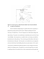
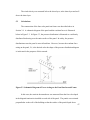
of wind forces as they interact with a bluff body. Figure 2.1, below, illustrates wind flow
over a low-rise buildings with flat roofs and a parapet along the roof edge. As wind
8
flows toward the building it eventually impacts the windward face and forms a separation
at the parapet (Holmes 2001). The wind flow below this separation layer, also called the
shear layer, is extremely turbulent. The wind flow above the shear layer is streamlined.
The region of turbulent air below the shear layer is called the recirculation region.
Within the recirculation region, there are significant net uplift forces generated near the
edge of a building with a flat roof. This uplift force dies down or decreases as the
distance from the edge of the building increases and the air flow reattaches to the roof.
ASCE7-10 accounts for this uplift pressure over a distance of 0.4 times the height of the
building or “10 percent of the least horizontal dimension of the building, whichever is
smaller” (ASCE-7 2010).
Figure 2.1 Principles of Wind Flow against a Bluff Body
ASCE-7 uses a probabilistic approach to determine design loading on structures.
The basic design wind speed values provided in the maps were determined using the
three-second gust wind speed with a certain percentage of probability of exceedance over
9
a specified time period. For example, in ASCE7-10, for a risk category II building (or
other structure), the wind speeds provided correspond to a 7% probability of exceedance
in 50 years (ASCE7 2010). Based on this methodology, the value of the wind pressure
for solar panels located on the flat roofed structures will have to be adjusted by several
factors to determine the appropriate value to use for design. This same methodology will
be used to produce design curves and external pressure coefficients and other factors that
are suitable for the design of solar collectors on buildings with flat roofs.
2.4
Wind Tunnel Studies
The first wind tunnel study concerned with solar collectors was conducted at the
end of the 1970’s in Bucharest. The focus of the study was on ground mounted solar
panels. It was determined that when solar panels are placed in an array, or groups, the
collectors located in the middle of the array were shielded by the collectors that were
installed in the first row (Radu 1986). This research was continued in the boundary layer
wind tunnel at Colorado State University (CSU). Further research at CSU determined
that arrays of solar panels experienced smaller forces than individual panels. This
particular study also determined that when solar panels were mounted in an array, there is
a significant force applied to collectors caused by the channelization of wind flow
between them. (Radu 1986).
At Texas A&M University, one of the first studies was conducted concerning
arrays of solar collectors mounted on flat roofs of existing buildings. The study
concluded that the first line of solar collectors provided a shielding of successive rows of
collectors in the array. However, it was later noted that there was “no satisfactory
10
attempt was made to simulate the boundary layer and the building on which the collectors
were mounted” (Radu 1986).
In 1984, additional research was conducted in the wind tunnels of Issay, Romania
(Radu 1986). This research was primarily concerned with the determination of pressure
coefficients on the surface of solar collectors mounted on the fat roofs of five story
buildings. The five story building was modeled with a rigid diaphragm and the building
and solar collector panels were scaled to 1:50. The panels were mounted at the center of
the roof with a 30° tilt angle with respect to the horizontal roof surface. The wind
direction was measured from 0° to 360°. Pressure taps were installed on the upper and
lower surfaces of the collector panels to determine the net pressure applied to the surface
of the collector. Pressure taps were also installed on the building roof surface and the
walls in order to facilitate a comparison between measured pressure coefficients and the
values provided by the building code. An urban exposure category was idealized in the
boundary layer wind tunnel so that the pressure coefficients measured could be compared
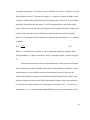
to other studies. Smoke was introduced wind tunnel (Figure 2.2) and it was observed that
as the air collided with the windward face of the building at the roof level, the “passage
of horizontal air streams” was prevented “giving rise to a shelter effect for the first rows
of solar panel collectors (Radu 1986).
11
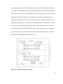
Figure 2.2 Smoke Visualization Used in the Boundary Layer Wind Tunnel.
Photo used from the 1986 Radu study (Radu et al. 1986, used with permission).
In fact, the study determined through the testing of numerous arrays with many
collectors mounted in the longitudinal direction of the wind that the panels prevented
flow re-attachment on the surface of the roof. The dominant resultant force acting on the
surface of the panels was uplift and the panels caused “increased turbulence over the
entire roof area.” The research provided values of pressure coefficients that were
measured across the panels that varied from +0.7 to -0.9. Where a positive force
coefficient represents pressure acting toward the surface of the panel and a negative
pressure coefficient is used where the pressure is acting away from the surface of the
12
panel. The study concluded that more testing was necessary particularly with respect to
varying exposure categories modeled in the wind tunnel.
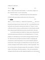
Since that time, research has continued in boundary layer wind tunnels. Figure
2.3 below depicts the many factors that have been considered in previous wind tunnel
studies which affect results of the model including building height (z), the height of the
panel (a), the slope of the roof surface, the slope of the panel (), the distance the panel is
located with respect to the windward edge of the building (c), as well as the wind speed
and direction. The presence and height of parapets can also affect the resulting net
pressure applied to the face of the panel.
Figure 2.3 Solar Collector Mounted on a Building with a Flat Roof and a Parapet
13
Many of these items have been studied by solar panel manufacturers, but the
results of these studies are typically not available in the public domain. One study,
conducted by Sun Link, a manufacturer of solar panels, determined that the design wind
pressures calculated using the methods currently provided in ASCE7 are un-conservative.
It is common for solar panels to be mounted on roof tops in an array. An array of solar
panels is used, rather than individual collectors, simply to increase the tributary area of
load acting on the panels. It is widely known that wind pressure is greater over a smaller
area than a larger one. The solar panels or arrays of solar panels are attached to an
existing roof structure with minimal connections or by a second means of attachment.
This secondary method of attachment reduces the weight of the system of solar collector
panels and support frames so the system can be held down on the roof’s structure with
ballast sufficient to resist the uplift force during a design wind event (Tilley 2012). The
study found that the pressures that developed on the roof were well in excess of 15
pounds per square foot (psf), even in a mild wind event; therefore the uplift pressures
could be well in excess of this value during a design wind event. Very few roofs, if any
provide sufficient ballast to resist 15 psf of uplift pressure.
At the 2012 Structures Congress, Dr. Ted Stathopoulos of Concordia University,
Montreal, Quebec, Canada, presented a paper summarizing the various values of pressure
coefficients that were measured in four different wind tunnel studies (Stathopoulos 2012).
The comparison included the results provided in the Radu study, published in 1986, and
three other studies conducted in 2011. The conclusion of Dr. Stathopoulos was that in
there was poor agreement between the results of these four wind tunnel studies. There
14
was very little correlation between measured values for the pressure coefficient, even
when the solar collector panels were mounted at the same tilt angle and the wind was
blowing from the same direction (Stathopoulos 2012). It is clear that despite the
numerous studies that have previously been conducted in the wind tunnels, more research
and validation is necessary to determine design values of the pressure coefficient on flat
roof mounted solar panels.
Recently, the Structural Engineers Association of California (SEAOC) developed
a “Wind Loads on Solar Collectors Subcommittee” (SEAOC 2012). The specific
purpose of this committee was to develop design procedures for wind loading applied to
solar collectors arrays on “flat roof low-rise buildings” in the interim period until these
design procedures are published in the ASCE-7 standard. As there may be a significant
period of time before the codification process is complete, the committee published
Figures 2.4 & 2.5 below to provide guidance and design values that can be used in
combination with the equations provided in ASCE7-05 or ASCE7-10. The design
procedure outlined in Figure 4, below, is valid for solar panels mounted on flat roofed
buildings with a tilt angle, ω, between 2° and 10° and a height, h1 greater than 10”. For
tilt angles less than 2° (basically flat), the uplift pressures determined from the ASCE710 components and cladding methods are allowed. The document also offers guidelines
for placement of panels with relation from the roof’s edge and there are several
adjustment factors included for array edge increase, parapet height and chord length. The
basic equation to compute the velocity pressure is
(
)
(1.3)
15
Where qh = velocity pressure at mean roof height and GCrn = combined net pressure
coefficient for solar panels.
It was observed that the values for the net pressure coefficients acting on the face
of the solar panels (+/-) GCrn was significantly greater than the external pressure
coefficients provided in Figure 30.8-1 in ASCE7-10 because they are distributed over a
significantly larger distance than 0.4h (where h is the height of the building) or 10% of
the least horizontal dimension which is used in ASCE7 for low rise buildings. The
committee determined that the distance “a,” (length of horizontal distribution of load) as
referred to in ASCE7-10 for solar panels mounted on flat roofed buildings, was five times
the distance of 0.4h. The committee determined that the value of “a” that is appropriate
for the design of solar panels on flat roofed building structures is twice the building
height. The committee explains that the difference is due to the roof and the solar panels
being “vulnerable to different phenomena. The roof is mainly vulnerable to the
difference between the pressure within the building and that above the roof. Solar panels
mounted on the roof are vulnerable to the speed of the wind approaching the panel.”
Because the typical tilt angle of solar collectors mounted on roofs is between 15° to 35°,
the panels are particularly vulnerable to the vertical uplift component of the wind. As
mentioned earlier, when the wind impacts the windward edge of the building a separation
point is developed and a recirculation region lies beneath. This increased uplift force on
the roof decreases as it gets further away from the edge of the building. This
phenomenon does not vary with wind speeds and thus the edge zone lengths have been
adjusted accordingly to account for this fact. Note that the values of the GCN at zone 0
16
are much smaller than at zones 1-3, presumably due to the shielding of these panels by
the first line of solar panels in the array as discussed and discovered in previous wind
tunnel studies.
17
Figure 2.4 Design GCp Values Published by SEAOC, August 2012 (SEAOC 2012,
used with permission)
18
Figure 2.5 Figure 29.9-1 from SEAOC Document
Part 2 of SEAOC Document “Wind Loads on Low Profile Solar Photovoltaic Systems on
Flat Roofs published in Draft format on March 28, 2012 (SEAOC 2012, used with
permission).
19
2.6
Conclusions
Although the amount of research that has been previously conducted is abundant,
the results of those tests are proprietary; the data measured from them is not available to
the public or to code writers for publication. SEAOC has recently commissioned a Wind
Subcommittee on Solar Photovoltaic Systems to publish the data obtained from these
numerous wind tunnel studies and provide design pressure coefficient curves. However,
as previously noted, the results of these tests provide design values that are not in
agreement with one another. This discrepancy could be due to many factors including
the difficulty in obtaining a proper scaled model that accurately represents the actual
stiffness and material properties of the panel itself (Tilley 2012). Because of this, it is
recommended that full-scale testing be conducted on flat roof mounted solar panels to
validate the pressure coefficients which have been determined from these many wind
tunnel studies and provided in the draft report written by the SEAOC subcommittee. Full
scale testing has been avoided in the past for many reasons. For example, when
conducting a full scale test, the researcher is left to wait for Mother Nature to produce
sufficient wind gusts (which may take a significant amount of time), unlike a wind tunnel
where the results can be generated in several hours. The testing equipment and solar
panels are outdoors and therefore are effected by temperature effects such as thermal
expansion and contraction of the frame. In a wind tunnel study, the solar panels can be
oriented in many directions and rotated on a turntable to study the effects of wind from
all directions; in full scale testing the solar panels must be placed in one orientation and
location and studied for an unpredictable period of time until favorable results are
20
obtained. Despite the complications involved with full scale testing, it is a necessary
component to validating the pressure coefficients determined from wind tunnel studies.
In an effort to provide data for comparison with past and future wind tunnel studies and
numerical analyses, full scale testing has been conducted at the University of Colorado
Denver.
21
3.
Panel Design, Location and Installation
3.1
Description
Initially three faux solar panel test frames were proposed and designed for the
purposes of this study (Dowds et al. 2012). The test frames were designed to emulate a
solar panel and measure the forces they were subjected to near the edge windward edge
of a flat roof. The panels were labeled Panel A, Panel B, and Panel C. Panel A was
designed so that the entire panel would be encompassed within the recirculation region
below the shear layer. Panel B was designed so that the midpoint of the face of the panel
would intersect the shear layer. Panel C was designed so that the entire panel would be
located above the shear layer. Once the design process began and the dimensions of the
three panels were determined and the uplift forces on each leg of the panel were
calculated, it was determined that Panel C was unfeasible. The height of Panel C would
have been unrealistic and therefore it was decided to construct only Panels A and B. The
panels were installed on the roof of the Events Center building at the University of
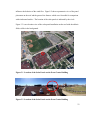
Colorado Denver’s Auraria campus as shown in Figure 3.1 below. The building is
oriented in the northwest direction. The panels were installed parallel to the northwest
face of the building and perpendicular to the prevailing wind direction. This location and
building was chosen due to its similarity to other buildings which have been modeled in
previous wind tunnel studies. These similarities include the building’s flat roof and
parapet, the large, open field located northwest of the building in the prevailing wind
direction and the lack of roof top obstructions in the vicinity of the panels which could
22
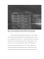
influence the behavior of the wind flow. Figure3.2 shows a panoramic view of the panel
placement on the roof and the general site features which were favorable for comparison
with wind tunnel studies. The location of the solar panels is indicated by the circle.
Figure 3.3 is an elevation view of the solar panel installation on the roof with the athletic
fields visible in the background.
Figure 3.1 Location of the Solar Panels on the Event Center Building
Figure 3.2 Location of the Solar Panels on the Event Center Building
23
Figure 3.3 Location of the Solar Panels on the Event Center Building
3.2
Wind Load
The Auraria campus is located in downtown Denver, Colorado. The site elevation
is approximately 5200 feet. A special wind region exists in Colorado, the easternmost
boundary of which is approximately defined by Interstate 25. The Auraria Campus,
shown in Figure 3.4 below, is located just east of this boundary.
24
Figure 3.4 Site Location of the University of Colorado Denver
The Auraria Campus, home to the University of Colorado Denver, is bordered by a
special wind region on its western boundary. The site campus location is indicated by the
star.
The prevailing wind direction for the site is from the northwest which is
approximately broadside to the building. The elevation at the roof of the Events Center
building on campus is approximately 5,248 feet. The height of the building is
approximately 38 feet. The exposure category is B according to the definitions set forth
in ASCE7-10. The design wind load on the solar panel test frames was approximated
using section 30.8.2 of ASCE7-10. In absence of guidance from ASCE-7 regarding the
design wind loads on solar panels it was assumed that this section closely depicted the
interaction between the wind and the panel frame. Section 30.8.2 is used for the design
25
of components and cladding wind loads on “open buildings with monoslope, pitched, or
troughed roofs” (ASCE7 2010). The basic wind speed used was 115 mph according to
Figure 26.5-1A of ASCE7-10 for Risk Category II Buildings. The wind load was
reduced by 80 percent according to the provisions for short duration installations in
chapter 6 of ASCE-37. According to this standard, the basic wind speed may be reduced
by 80 percent for a construction period of six weeks to one year (ASCE37 2002).
3.3
Design Calculations
The design wind pressure as determined above was applied to the surface of the
panel. The resultant net force acting on the face of the panel was computed. Once the
resultant force was known, the uplift force in the legs of the panel frames and the tension
ties was computed. It should be noted that the resultant uplift force in the panel legs
calculated by this method considers sliding only, which is the force acting in the
horizontal direction, perpendicular to the legs of the panel. In this case the vertical uplift
force on the panel legs is irrelevant (except to determine the weight of the hold downs)
because the resultant force acting on the face of the panel is calculated using the
horizontal component of the force from the diagonal tension tie. Throughout the design
process of the panel frame consideration was given to both sliding and overturning of the
panel and the panel legs were designed for the worst case vertical uplift force and
bending moments.
26
3.4
Faux Solar Panel Test frame
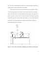
The height of the panels was determined by the location of the shear layer four
feet from the outside edge of the parapet. It was assumed that the slope of the shear layer
slope was 2:1 horizontal to vertical from the leading edge of the parapet (SEAOC 2012).
The slope of the surface of each of the panels was selected to be 30 degrees to maximize
the wind effects on the panel. The surface of each panel was constructed from 3/8”
plywood with dimensions of two feet wide by four feet long. The vertical legs of each
panel were constructed from 16 gage, one inch square tube steel. An overview of the
construction of panel A is illustrated in Figure 3.5 below.
Figure 3.5 Panel A Construction Overview
Because the shear layer develops at a 2:1 horizontal slope with respect the edge of
the roof, the height of panel A was much shorter than panel B. As illustrated in Figure
27
3.6 below, the height of panel B is almost twice that of panel A. Figure 3.7 is a
photograph of panel B as constructed.
Figure 3.6 Panel B Construction Overview
Figure 3.7 Panel B Construction Overview
28
3.5
Connection Details
A ¼ inch eye bolt was installed through a hole drilled through the top and bottom
of the panel legs. Tension ties were created from 7/16 inch diameter threaded steel rod
which was through bolted to a strain transducer through a ½ inch diameter hole. The
tension ties were installed at an angle of 6 degrees for panel A and 45 degrees for panel
B. The slope of the tension ties was determined once the height of each panel was
known. Nuts were fastened to each side of the wall of the strain transducer to allow for
adjustment and pretensioning of the ties in the field. The tension ties were connected to
the panel legs by a coupler nut. A 5/16” diameter hole was drilled through one end of the
7/16” diameter coupler nut which was threaded onto the tension tie and attached to the
¼” eyebolt at the top and bottom of the panel legs as shown in Figure 3.8. It was
intended that this connection remain a pin-end connection in order to direct all horizontal
components of force into the diagonal tension tie, where the force could be monitored via
the strain transducers. The strain transducers were fabricated from three inch diameter by
two inch wide steel rings with strain gages adhered to their inside surfaces. A cable brace
was installed, slightly slack in the opposite direction of the tension tie to provide stability
for the frame for the case of wind blowing in the opposite direction as illustrated in
Figure 3.5.and 3.6. The top of the panel legs were connected to the 3/8” plywood panel
surface via ½” diameter bolts through 1x1x1/8” steel angles that were six inches long.
The same connection was used at the base of the panel legs to connect them to a wood
2x6 laid flat. The heads of the bolts were countersunk into the bottom of the 2x6 to
prevent damage to the surface of the roof.
29
7/16 THREADED
ROD
Figure 3.8 Panel Frame Connection Details.at the Diagonal Tension Ties
Figure 3.9 Panel Frame Connection Details in the Short Dimension
30
Figure 3.10 Close-Up View of Short Direction Panel Frame Connection Details
3.6
Assembly and Installation
Prior to construction, shop drawings were produced for the steel components of
the panel frame and provided to the Electronics Calibration and Repair Lab at the
University of Colorado Denver. The steel components were fabricated according to the
shop drawings. The panels were assembled prior to installation on the roof of the Events
Center Building. Once the panels were assembled, cable cross bracing was installed in
the short direction of the panel legs. The cross bracing provided stability of the frame in
the short direction of the panel. Once the panels were assembled, they were transported
to the roof of the Events Center building where they were placed upon a 10’x10’ pad of
concrete pavers to distribute the load from the panels over the existing precast concrete
double tee roof framing system. The uplift force on each of the panel legs was resisted
by sand bags which were provided in lieu of a direct connection between the panels and
31
the existing roof structure. Once the panels were placed in the location shown in Figure
3.11 below, 50 lb. sand bags were stacked on the ends of the 2x6s until the desired hold
down force was achieved. Upon installation of the faux solar panels, it became clear that
the height of the stacked sand bags could influence the air flow surrounding the faux
solar panels, particularly panel A. In an effort to reduce the changes in the air flow, the
height of the sand bag stack was limited to the height of the top of the parapet. However,
for panel A, this was approximately half its height. Three anemometers were used to
measure the wind speed at different locations. One of the anemometers was positioned
below the shear layer, the second at the assumed location of the shear layer, and a third
well above the assumed location of the shear layer.
Figure 3.11 Panel Layout and Location
32
4.
Instrumentation
4.1
Introduction
The desired output was measured using a data logger and various instruments as
described below.
4.2
Data Logger
Data was collected using a Campbell Scientific CR5000 data logger. The data
logger was calibrated by Campbell Scientific prior to use. An external battery was used
to power the data logger in conjunction with a solar panel which was used to charge the
external battery. The data was stored on a PC card to decrease the number of trips to the
site to download data and also to reduce the downloading time. During the research, the
data logger was placed within a sheet metal enclosure box to protect it from wind, rain
and snow. The data logger was programmed to record the strain, wind speed, and wind
direction at one second intervals. The data was then post-processed to average the wind
speeds and associated strains over three second and nine second intervals.
33
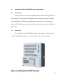
Figure 4.1 Campbell Scientific CR5000 Data Logger
Figure courtesy of Campbell Scientific, Inc., Logan Utah.
4.3
Solar Panel
A Campbell Scientific SP20 solar panel, shown in Figure 4.2, was used to charge
the CR5000 data logger’s external battery so that continuous data records were gathered.
The panel was oriented to the south to gain maximum sun exposure.
34
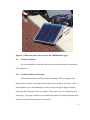
Figure 4.2 SP20 Solar Panel Used to Power the CR5000 Data Logger
4.4
Strain Transducers
Six strain transducers were fabricated for use in this experiment; the transducers
were labeled A-F.
4.4.1
Strain Transducer Fabrication
Each strain transducer was fabricated by mounting a 350Ω strain gage to the
inside surface of a three inch diameter steel ring as shown in Figure 4.3 below. Holes, ½
inch in diameter, were drilled through two sides of the steel ring 90 degrees from the
strain gage and 180 degrees from one another. Three lead wires were soldered to each
strain gage. The gages were then covered with small squares of silicone and taped down
to the steel ring with electrical tape for protection.
35
Figure 4.3 Strain Transducer
4.4.2
Strain Transducer Calibration
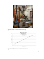
The strain transducers were calibrated prior to use in the using an MTS machine
in the UCD structures lab. For calibration purposes one foot long sections of 7/16 inch
diameter all thread were bolted to each side of the strain transducer (the same material
which was used for the diagonal tension ties in the solar panel frame). Figure 4.4 shows
the strain transducer arrangement in the MTS machine during calibration. Once the
transducers were calibrated load versus strain curves were developed for each gage. The
calibration curves for all six of the transducers (A-F) are provided below in Figures 4.5
through 4.10.
36
Figure 4.4 Strain Transducer Calibration Set-Up
Figure 4.5 Calibration Curve for Strain Transducer A
37
Figure 4.6 Calibration Curve for Strain Transducer B
Figure 4.7 Calibration Curve for Strain Transducer C
38
Figure 4.8 Calibration Curve for Strain Transducer D
Figure 4.9 Calibration Curve for Strain Transducer E
39
Figure 4.10 Calibration Curve for Strain Transducer F
4.4.3
Strain Transducer Installation
One strain transducer was connected to the diagonal tension tie of each leg of the
panel. The fifth was used to measure change in strain caused by thermal effects only.
The sixth strain transducer served as a backup if there was a malfunction with one of the
other five transducers. The strain transducers were covered with foil insulation to guard
against solar radiation heating them above the ambient air temperature. Strain
transducers A and B were connected to panel A, strain transducers B and E were
connected to panel B, and strain transducer F was not connected to a panel but used to
measure change in strain due to thermal effects. Figure 4.11 below shows the solar panel
layout, the strain transducers are labeled below the corresponding panel leg they were
connected to.
40
Figure 4.11 Strain Transducer Instrumentation Plan
4.5
Anemometers
Three RM Young 3101 Wind Sentry Anemometers were used to record the wind
speed. “Wind speed is measured with a three cup anemometer. Rotation of the cup when
produces an ac sine wave voltage with frequency proportional to wind speed (Campbell
Scientific 2007). The anemometers are shown in Figure 4.12, below.
41
Figure 4.12 RM Young 3101 Anemometer
Courtesy of Campbell Scientific, Inc., Logan, Utah.
4.6
Wind Direction Sensor
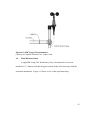
A single RM Young 3301 Wind Sentry Vane was mounted to a cross arm
attached to a ¾” diameter schedule 40 pipe located well above the shear layer with the
associated anemometer. Figure 4.13 shows a view of the experiment setup.
42
Anemometer
Vane
Panel B
Panel A
Figure 4.13 Overview of Anemometer and Vane Installation
4.7
Thermocouple
Campbell Scientific A3537 Type T thermocouple wire was used to record the
ambient air temperature. The recorded temperatures were then compared with the daily
reported temperatures gathered from the National Climatic Data Center records (U.S.
Department of Commerce 2013) to confirm the accuracy of the readings. The Type T
Thermocouple is made from a copper and constantan wire. The thermocouple wire was 2
feet long and routed outside of the data logger enclosure box to record the ambient air
temperature rather than the panel temperature within the data logger enclosure.
43
4.8
Interval Timer
An SDM-INT8 interval timer, manufactured by Campbell Scientific was used to
capture wind speed data from the third anemometer. The interval timer has eight
channels which can be programmed to “output processed timing information to a CR5000
data logger” (Campbell Scientific 2011).
4.9
Software
RTDAQ 1.1, software provided by Campbell Scientific, was used with the
CR5000 data logger to record all measurements. RTDAQ 1.1 (Campbell Scientific 2001)
is compatible with computers running Microsoft Windows XP, Windows Vista or
Windows 7 operating systems. For the purposes of this experiment, a Dell Inspiron 5423
Laptop was used with Windows 7 as the computer’s operating system.
Short Cut and CRBasic Editor (Campbell Scientific 2001) were used to create the
program used to record the measurements from the strain gages, anemometers,
thermocouple and the wind direction sensor. Both Short Cut and CRBasic Editor were
provided with the RTDAQ 1.1 software to be used in conjunction with the CR5000 data
logger. A brief instruction for use of the CR5000 data logger has been provided in
Appendix A. Instructions to create a program in Short Cut are provided in Appendix B
and instructions to edit the program in CRBasic Editor are provided in Appendix C. The
program created in Short Cut and edited in CRBasic Editor is provided in Appendix D.
The data tables generated by the program listed a record number, date and time stamp,
strain output from the five strain transducers, wind direction, wind speed from the three
anemometers, and the ambient air temperature..
44
5.
Theory
5.1
Introduction
Numerous wind tunnel studies have been conducted to determine various design
parameters for individual solar manufacturers. When a wind tunnel study is performed,
typically pressure taps are used to directly measure the pressure distribution across the
face of the panel. The pressure coefficient, Cp, can be determined by calculating the net
pressure across the upper and lower surface of the panel. For the purposes of this study, a
test frame was developed to calculate the net force acting on the face of the panel.
Therefore instead of pressure coefficients, force coefficients, CF, were calculated from
the measured data. The methodology used to calculate the force coefficients is described
as follows.
5.2
Wind Interaction with the Panel
As discussed in Section 2.3, as wind flow impacts a bluff body, such as a building,
several phenomena occur. A separation occurs at the roof edge and a region of turbulent
air flow develops on the surface of the roof over a certain distance. For the purposes of
this study it was desired to investigate the force coefficients developed when a solar panel
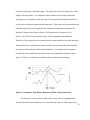
was placed within the shear layer. Panel B was designed so that the midpoint of the face
of the panel would intersect the shear layer. It was assumed that a secondary separation
point and shear layer and recirculation region would develop on the panel’s face as
depicted below in Figure 5.1. Panel A was placed below the shear layer therefore the
entire panel was located within the recirculation region as illustrated in Figure 5.2.
45
Figure 5.1 Schematic Diagram of Wind Interaction at Panel B
Figure 5.2 Schematic Diagram of Wind Interaction with Panel A
46
The wind velocity was measured below the shear layer, at the shear layer and well
above the shear layer.
5.3
Calculations
The construction of the faux solar panel test frames was described above in
Section 3.4. A schematic diagram of the panel and the resultant forces is illustrated
below in Figure 5.3. In Figure 5.3, the pressure distribution is illustrated as a uniformly
distributed load acting over the entire surface of the panel. In reality, the pressure
distribution across the panel is not at all uniform. However, because the resultant force
acting on the panel, FR, is the desired value the shape of the pressure distribution diagram
is irrelevant for the purposes of this research.
Figure 5.3 Schematic Diagram of Forces Acting on the Panel Surface and Frame
In this case, the strain in the transducers was measured from the force developed
in the diagonal tension ties installed on each side of the panel. The panels were oriented
perpendicular to the wall of the building so that the surface of the panel sloped down
47
toward the roof surface. As noted previously a tilt angle, p equal to 30 degrees was used
for both panels A and B. The tension tie angle, is equal to 6 degrees for Panel A and
45 degrees for Panel B measured from the horizontal surface of the roof. A net resultant
wind force imposed on the solar panel, FR, will act perpendicular to the surface of the
panel. From the measured strain in the tension ties, the resultant wind force acting on the
surface of the solar panel can be calculated by summing the forces in the horizontal
direction. The equation for the resultant force from the measured Strain, FR, is calculated
as follows
(5.1)
Where FR = resultant force on panel, T =force in diagonal tension tie measured from
strain transducers,  =angle of tension tie, and p =tilt angle of panel, as shown in Figure
5.3.
From the measured wind velocity, the resultant force on the net area of the panel
due to the dynamic pressure from the wind velocity is determined by equation 5.2 below.
An instrument was not available to measure the barometric pressure; therefore the
uncorrected barometric pressure was obtained from the National Climactic Data Center
website using the data measured at Denver International Airport, which was considered
to be the closest weather station (U.S. Department of Commerce 2013). As with the FR
calculations, Fvel press was calculated using the difference between two measured velocity
48
readings, two seconds apart
(5.2)
Where ρ = density of air (uncorrected for altitude), V = wind velocity averaged over a
three second interval and A = net area of panel surface
The force coefficient, CF, is determined from the ratio of the resultant force
measured from the strain transducers and force due to the velocity pressure
(5.3)
Where CF = net force coefficient, FR = resultant force on panel and Fvel press = the force on
the panel from the dynamic pressure from the wind. The CF was calculated based on the
actual surface area of the panel, not the projected vertical area. The term CF, or force
coefficient is used in lieu of pressure coefficient because it is derived from the measured
forces acting on the panel rather than the net pressure across the surface of the panel.
As previously mentioned, the resultant force acting on panel is determined from
strain measurements generated from the force in the diagonal tension ties. The strain
transducers were fabricated using a steel ring with a strain gage mounted to the inside
face. Because the forces developed in the tension ties and the corresponding strain
measurements are small, the ring transducers were used to mechanically amplify the
measured strain. If the strain gages were mounted directly to the legs of the legs of the
test frame, the changes in strain would be so small, they would be imperceptible. There
are several factors which could impact the output of the strain transducers. The thermal
output of each strain gage is affected by temperature. Vishay, who manufactured the
strain gages used in this study, provided a graph and an equation to correct the measured
49
strain from each gage for thermal output. The gage factor of the strain gages also varies
slightly with temperature. To complicate matters further, the steel ring to which the
strain gages were mounted as well as the legs of the panel and the diagonal tension ties
are all subject to thermal expansion and contraction. Temperature was measured through
a thermocouple which was compared to the ambient air temperature reported on the
National Climactic Data Center website (U.S. Department of Commerce 2013).
However, the effect of solar radiation on the various components was unknown.
Therefore, if the resultant force measured from the strain transducers was used directly to
determine the force coefficient, the results would be in error unless the measured strain
was corrected for the thermal effects described above. A technique was developed to
calculate the force coefficient on the panel which was independent of thermal effects.
Figure 5.4 below is a schematic time history used to illustrate this technique.
Figure 5.4 Schematic Time History Diagram of Wind Velocity and Strain
For each gust, a plot can made of the wind velocity and corresponding strain
measured from the strain transducers over a specified time interval. When gusts occur,
50
there is a peak in the wind velocity diagram and a corresponding peak in the measured
strain. This occurs each time the wind strikes the panel from a particular direction over
the duration of the gust. In this case, that wind direction was set to be 180 degrees. The
force coefficient, CF, was calculated by taking the difference between the measured
strains over a two second interval and dividing that value by the change in the square of
the velocities over the same time interval
(
(
)
)
(5.4)
Where CF = net force coefficient, T = force calculated from the measured strain in the
tension ties,  =angle of tension tie, and p =tilt angle of panel, ρ = density of air and V =
wind velocity. The thermal effects on the steel elements of the panel frame as well as the
thermal output of the strain gages are considered to be negligible over the short duration.
The tilt angle of the panel, the angle of the tension tie, the barometric pressure and the
panel area are all known quantities. Thus the force coefficient is directly proportional to
the change in strain over a two second time interval divided by the change in the
velocities squared over the same two second time interval shown in equation 5.4. The
two second interval was arbitrarily selected for convenience. It should be noted that the
velocities used to calculate the force coefficients were averaged over a three second
interval and correspond to a 3-second gust wind speed. Therefore, the CF calculated
using equation 5.4 is inclusive of the gust effect factor, G. The term CF was used rather
than GCF because the force coefficients were determined from direct measurements and
therefore the gust effect factor, G, was assumed to be equal to 1.0.
51
Initially, it was assumed that the largest force coefficients would be obtained
when the wind direction was perpendicular to the panel. The data was filtered so that
force coefficients were calculated when the wind was blowing from the direction of
interest. A tolerance of 10 degrees was allowed. Therefore CF values were calculated
when the wind direction was 170 degrees to 190 degrees as illustrated in Figure 5.5
CF
below.
Figure 5.5 Filtered Wind Direction for CF Calculation
To validate the initial assumption regarding the maximum force coefficients, two
additional wind directions were also investigated. The additional wind directions
considered were 20 degrees and 45 degrees from the axis perpendicular to the panel. A
10 degree tolerance was also allowed.
52
53
6.
Results and Discussion
6.1
Introduction
For purposes of this thesis, the findings from panel B, the panel located within the
shear layer are reported upon. The results from panel A were inconclusive. The wind
velocity, direction and strain were collected using a sampling interval of one second.
Data was post processed over three-second rolling averages.
6.2
Results
The results from the data analysis from the wind direction perpendicular to the
face of the panel (corresponding to 180°) are presented in the time histories below in
Figures 6.1 and Figures 6.3 through 6.9. A summary of the force coefficients, CF,
calculated for the selected 400 second time history plotted in Figure 6.1 is provided in
Table 6.1. The force coefficients in Table 6.1 were calculated from three second rolling
averages as mentioned above. The numerical values for strain plotted in the following
figures are irrelevant, because all of the CF values were calculated from forces
determined from changes in strain.
54
Figure 6.1 Wind Velocity, Strain and Calculated CF Values from 4/14/13 Data
The values were taken from a selected record averaged using a 3-second rolling average.
55
Table 6.1 Summary of CF determinations from Figure 6.1 within wind direction
tolerance for 3-second rolling averages
CF – 3-second Average
18.7
2.1
1.3
0.6
9.9
2.0
1.3
0.6
5.2
1.9
1.2
0.5
4.2
1.9
1.1
0.5
3.8
1.9
1.0
0.5
3.8
1.9
1.0
0.4
3.1
1.9
0.9
0.4
2.8
1.7
0.8
0.3
2.7
1.6
0.8
0.3
2.7
1.6
0.8
0.3
2.6
1.6
0.8
0.2
2.5
1.5
0.7
0.2
2.4
1.4
0.7
0.1
2.2
1.4
0.7
2.1
1.3
0.7
56
The wind direction data over the same time 400 second time history depicted
above has been plotted below, in Figure 6.2. The CF values calculated using the 3-second
averaged wind velocity from all directions are plotted along the x-axis for comparison
with Figure 6.1 to further illustrate how the CF values were filtered.
Figure 6.2 Results of Wind Direction Plotted Versus CF from April 14, 2013
CF values for all wind directions are shown here.
The 400 second time history and CF values computed from 9-second rolling
averages are shown below in Figure 6.3 and Table 6.2 for a wind direction perpendicular
to the panel. Note that Figure 6.3 was created from the same data over the same time
57
interval as depicted in Figure 6.1using a 9 second rolling average in an attempt to reduce
the variation in the curve and the variation in the force coefficients.
Figure 6.3 Wind Velocity, Strain and calculated CF Values from 4/14/13 Data
The values were taken from a selected record averaged using a 9-second rolling average.
58
Table 6.2 Summary of CF determinations from Figure 6.3 within wind direction
tolerance for 9-second rolling averages
CF – 9-second Average
13.8
1.7
0.9
0.5
11.5
1.6
0.8
0.5
7.1
1.5
0.8
0.5
6.5
1.5
0.8
0.4
4.0
1.4
0.7
0.4
3.6
1.3
0.7
0.3
2.2
1.3
0.7
0.2
2.2
1.2
0.7
0.2
2.0
1.2
0.7
0.2
2.0
1.1
0.6
0.1
1.9
1.1
0.6
0.1
1.8
1.0
0.6
0.1
1.8
1.0
0.6
0.1
1.7
1.0
0.5
0.1
1.7
0.9
0.5
Additional time histories are plotted below in Figures 6.4 through 6.9. Following
each time history plot, the filtered CF values for the 180 degree wind direction are
summarized in Tables 6.3 through 6.8.
59
Strain E
Strain E
Wind Velocity
CF
Figure 6.4 Time History of Wind Velocity and Strain with Corresponding CF
The records above were taken from a different time record on 4/14/13 and averaged over
a three second interval.
60
Table 6.3 Summary of CF determinations from Figure 6.4 within wind direction
tolerance for 3-second rolling averages
CF – 3-second Average
8.6
1.5
0.9
0.4
6.5
1.4
0.8
0.4
5.8
1.3
0.8
0.4
4.5
1.2
0.7
0.3
3.3
1.1
0.5
0.2
2.4
1.0
0.5
0.2
2.4
1.0
0.5
0.2
2.4
1.0
0.5
0.1
2.3
1.0
0.5
0.4
2.1
1.0
0.5
0.4
1.7
1.5
0.5
0.4
61
Figure 6.5 Time History of Wind Velocity and Strain with Corresponding CF
The time history diagram above is taken from data obtained on 4/14/13 and averaged
over a three second interval.
62
Table 6.4 Summary of CF determinations from Figure 6.5 within wind direction
tolerance for 3-second rolling averages
CF –3-second Average
11.9
2.1
1.1
0.4
9.2
2.1
0.9
0.4
6.6
1.9
0.8
0.3
5.6
1.8
0.7
0.2
5.6
1.6
0.7
0.1
3.8
1.5
0.6
3.4
1.5
0.5
2.9
1.4
0.5
63
Strain E
Strain C
Wind Velocity
CF
Figure 6.6 Time History of Wind Velocity and Strain with Corresponding CF
The time history diagram above is taken from data obtained on 4/14/13 and averaged
over a three second interval.
64
Table 6.5 Summary of CF determinations from Figure 6.6 within wind direction
tolerance for 3-second rolling averages
CF – 3-second Average
6.8
2.0
1.3
0.7
6.6
2.0
1.2
0.7
5.0
2.0
1.2
0.7
4.2
2.0
1.2
0.5
4.0
1.8
1.1
0.4
3.7
1.8
1.1
0.4
2.9
1.7
0.9
0.4
2.8
1.6
0.9
0.4
2.7
1.6
0.9
0.3
2.5
1.5
0.9
0.2
2.3
1.5
0.8
0.2
2.3
1.5
0.8
0.1
2.0
1.3
0.7
0.1
65
Strain C
Strain E
Wind Velocity
CF
Figure 6.7 Time History of Wind Velocity and Strain with Corresponding CF
The time history diagram above is taken from data obtained on 4/14/13 and averaged
over a three second interval.
66
Table 6.6 Summary of CF determinations from Figure 6.7 within wind direction
tolerance for 3-second rolling averages
CF – 3-second Average
14.2
2.4
1.0
0.5
5.1
2.3
0.9
0.5
4.9
2.2
0.9
0.5
4.7
1.9
0.9
0.5
4.0
1.8
0.9
0.3
3.7
1.8
0.8
0.3
3.6
1.6
0.8
0.3
3.0
1.6
0.6
0.2
2.8
1.5
0.6
0.2
2.6
1.1
0.6
0.2
2.6
1.1
0.5
2.4
1.0
0.5
67
Strain C
Strain E
Wind Velocity
CF
Figure 6.8 Time History of Wind Velocity and Strain with Corresponding CF
The time history diagram above is taken from data obtained on 4/14/13 and averaged
over a three second interval.
68
Table 6.7 Summary of CF determinations from Figure 6.8 within wind direction
tolerance for 3-second rolling averages
CF – 3-second Average
17.2
1.9
0.9
0.4
7.1
1.8
0.8
0.4
5.0
1.7
0.8
0.4
4.6
1.6
0.8
0.3
4.6
1.5
0.8
0.3
2.9
1.2
0.7
0.3
2.8
1.1
0.6
0.3
2.8
1.1
0.5
0.3
2.7
1.0
0.5
0.2
2.4
1.0
0.5
0.2
2.3
1.0
0.4
0.1
2.2
1.0
0.4
0.1
69
Strain C
Strain E
Wind Velocity
CF
Figure 6.9 Time History of Wind Velocity and Strain with Corresponding CF
The time history diagram above is taken from data obtained on 4/14/13 and averaged
over a three second interval.
70
Table 6.8 Summary of CF determinations from Figure 6.9 within wind direction
tolerance for 3-second rolling averages
CF – 3-second Average
9.1
2.4
1.3
0.6
9.0
2.2
1.2
0.5
7.5
2.2
1.2
0.5
5.1
2.1
1.1
0.5
4.6
1.9
1.0
0.5
4.0
1.9
1.0
0.3
4.0
1.7
0.9
0.2
3.7
1.7
0.9
0.2
2.9
1.6
0.8
0.2
2.9
1.6
0.8
0.1
2.8
1.4
0.8
0.1
2.7
1.4
0.8
2.7
1.3
0.7
2.6
1.3
0.7
71
In Figures 6.10 through 6.13, the time history diagrams have been plotted over a
400 second time interval for a wind direction 20 degrees from the perpendicular axis of
the panel (150 to 170 degrees). The corresponding CF values summarized in Tables 6.9
through 6.12 have been filtered for the same wind direction.
Strain C
Strain E
Wind
Velocity
CF
Figure 6.10 Time History of Wind Velocity and Strain with Corresponding CF
The time history diagram above is taken from data obtained on 4/14/13 and averaged
over a three second interval.
72
Table 6.9 Summary of CF determinations from Figure 6.10 within wind direction
tolerance for 3-second rolling averages
CF – 3-second Average
9.8
2.3
1.2
0.7
7.5
2.2
1.0
0.6
7.2
2.0
1.0
0.5
7.2
1.8
1.0
0.4
5.9
1.7
0.9
0.4
4.2
1.6
0.9
0.2
3.7
1.6
0.8
3.2
1.3
0.8
2.8
1.3
0.7
73
Strain C
Strain E
Wind Velocity
CF
Figure 6.11 Time History of Wind Velocity and Strain with Corresponding CF
The time history diagram above is taken from data obtained on 4/14/13 and averaged
over a three second interval.
74
Table 6.10 Summary of CF determinations from Figure 6.11 within wind direction
tolerance for 3-second rolling averages
CF – 3-second Average
11.1
2.1
1.2
0.8
8.0
2.0
1.1
0.5
6.6
2.0
1.1
0.5
6.3
2.0
1.1
0.4
5.2
1.7
1.1
0.4
3.7
1.7
1.1
0.3
3.1
1.4
1.0
0.3
2.6
1.4
1.0
0.2
2.5
1.3
0.9
0.2
2.3
1.2
0.9
0.1
2.2
1.2
0.8
0.8
75
Strain C
Strain E
Wind Velocity
CF
Figure 6.12 Time History of Wind Velocity and Strain with Corresponding CF
The time history diagram above is taken from data obtained on 4/14/13 and averaged
over a three second interval.
Table 6.11 Summary of CF determinations from Figure 6.12 within wind direction
tolerance for 3-second rolling averages
CF – 3-second Average
11.3
3.6
1.6
1.0
9.8
3.3
1.4
0.9
5.8
2.2
1.2
0.9
4.7
2.1
1.2
0.9
4.3
2.1
1.1
0.7
4.0
1.7
1.1
76
Strain C
Strain E
Wind Velocity
CF
Figure 6.13 Time History of Wind Velocity and Strain with Corresponding CF
The time history diagram above is taken from data obtained on 4/14/13 and averaged
over a three second interval.
77
Table 6.12 Summary of CF determinations from Figure 6.13 within wind direction
tolerance for 3-second rolling averages
CF – 3-second Average
8.4
1.9
1.0
0.8
7.5
1.6
1.0
0.6
5.4
1.6
1.0
0.5
5.3
1.5
1.0
0.5
4.4
1.5
0.9
0.4
3.6
1.3
0.9
0.3
3.1
1.2
0.9
0.2
2.7
1.2
0.9
0.2
2.6
1.2
0.8
0.8
2.4
1.0
0.8
0.6
78
Figures 6.14 through 6.16 are time history diagrams plotted over a 400 second
time interval for a wind direction 45 degrees from the perpendicular axis of the panel or
225 degrees as measured (215 to 235 degrees). The corresponding CF values
summarized in Tables 6.13 through 6.15 have been filtered for the same wind direction.
Strain C
Strain E
Wind Velocity
CF
Figure 6.14 Time History of Wind Velocity and Strain with Corresponding CF
The time history diagram above is taken from data obtained on 4/22/13 and averaged
over a three second interval.
79
Table 6.13 Summary of CF determinations from Figure 6.14 within wind direction
tolerance for 3-second rolling averages
CF – 3-second Average
11.1
1.4
0.8
0.4
6.9
1.4
0.8
0.4
6.7
1.3
0.7
0.4
5.1
1.3
0.7
0.4
3.6
1.2
0.7
0.3
3.0
1.1
0.7
0.3
2.8
1.1
0.7
0.3
2.6
1.1
0.6
0.2
2.1
0.9
0.6
0.2
1.9
0.9
0.5
0.2
1.8
0.9
0.5
0.2
1.8
0.9
0.5
0.2
1.6
0.8
0.5
0.1
1.4
0.8
0.4
0.1
80
Strain C
Strain E
Wind
Velocity
CF
Figure 6.15 Time History of Wind Velocity and Strain with Corresponding CF
The time history diagram above is taken from data obtained on 4/22/13 and averaged
over a three second interval.
81
Table 6.14 Summary of CF determinations from Figure 6.15 within wind direction
tolerance for 3-second rolling averages
CF – 3-second Average
15.4
2.4
1.2
0.6
7.5
2.2
1.1
0.5
6.8
2.1
0.8
0.5
3.9
1.7
0.8
0.4
3.8
1.6
0.8
0.4
3.7
1.4
0.8
0.4
3.5
1.4
0.7
0.3
3.2
1.3
0.6
0.3
2.5
1.3
0.6
0.3
82
Strain C
Strain E
Wind Velocity
CF
Figure 6.16 Time History of Wind Velocity and Strain with Corresponding CF
The time history diagram above is taken from data obtained on 4/30/13 and averaged
over a three second interval.
83
Table 6.15 Summary of CF determinations from Figure 6.16 within wind direction
tolerance for 3-second rolling averages
CF – 3-second Average
11.3
1.9
1.0
0.4
9.4
1.8
0.9
0.4
5.1
1.6
0.9
0.4
4.3
1.6
0.8
0.4
4.1
1.5
0.7
0.4
4.1
1.5
0.7
0.4
3.8
1.3
0.6
0.3
3.5
1.2
0.6
0.3
2.8
1.2
0.5
0.3
2.6
1.1
0.5
0.2
2.5
1.1
0.5
0.2
2.2
1.1
0.5
0.2
2.1
1.0
0.5
.
84
6.3
Discussion
The 400 second time interval was arbitrarily selected. Unlike wind tunnel studies
where the wind is constantly coming from one direction of interest, in full scale testing
the wind directions change rapidly over a short duration of time. The the 400 second
time interval was selected for the time histories above to illustrate the wind gusts which
occurred in the wind direction of interest over that particular 400 second time interval.
The initial assumption was that the maximum resultant force on the panel would
be produced by winds from the northwest, which was set to 180 degrees or perpendicular
to the panel. The force coefficients summarized in Table 6.1 ranged from a minimum
value of 0.1 to a maximum value of 18.7. Those force coefficients were based on a 3
second averaging of the measured wind speeds and strains for the time history record
shown in Figure 6.1. While several CF values are relatively high, the majority range from
approximately 0.6 to 2.2 for the 3-second rolling average.
It is observed that the wind velocity is highly variable over the relatively short
time duration. The wind velocity and measured strain are less variable when an
alternative averaging interval is selected. In Figure 6.2 a 9 second rolling average was
used to smooth out the variability in the data plot. Note that the CF values in Table 6.2
reflect that there is less variation than in Table 6.1. The CF values in Table 6.2 for the 9
second averaged data plotted in Figure 6.3 ranged from a minimum CF of 0.1 to a
maximum value of 13.8, however the majority range from 0.5 to 1.8.
We note that CF values as high as 10 are reported to “often occur” and up to 20
have occasionally been measured; however these values are associated with corner
85
vortices (Holmes 2007). This trend appears to also be correct for solar panels located in
the shear layer near the edge of a building with a flat roof. In Tables 6.1 through 6.8 the
force coefficients for the wind perpendicular to the face panel are summarized. Two of
the values were extremely high and their validity was questionable. These values were
18.7 and 17.2 found in Table 6.1 and 6.7 respectively.
Particular consideration was given to the validity of the CF values that were
calculated. Because CF is determined from the ratio of measured force divided by the
force due to the velocity pressure, the squared velocity term is always in the denominator
of the calculation. Therefore if the change in wind speed was relatively small combined
with a relatively large change in strain, the magnitude of the CF value would be large.
Conversely, when the change in wind velocity was relatively large combined with a
relatively small change in strain, the CF values would be small. It was decided that the
values of CF were relevant when the slope of the curves for the change in strain and the
change in wind velocity were in the same direction, that is the slope of both curves were
positive or both were negative. Force coefficients were rejected if a peak in the strain
diagram happened to occur where there was little change in velocity over the two second
time interval, producing an unreasonably large CF. Thus numerous data points were
filtered out as irrelevant. For example, in Tables 6.1 and 6.2 above, the overall sampling
interval for the data presented was 400 seconds. Using the filtering technique, only 60 CF
values were retained as relevant.
The 18.7 and 17.2 CF values could not be ruled out as invalid. It can be seen in
Tables 6.1 through 6.8 that force coefficients of 5-10 occur frequently based on a 386
second averaging of wind speeds. These values are well in excess of the values provided
in the SEAOC document. The nominal net pressure coefficients obtained from Figure
29.9-1 of that document are a maximum value of 3.6 (SEAOC 2012). However, this
document does not consider solar panels placed within the shear layer or near the edge of
a flat roof. In fact the SEAOC document explicitly states that panels should be placed
away from the edge of the roof at a minimum distance of four feet or twice the distance
between the height of the panel and the height of the parapet, whichever value is larger.
In this case, that minimum distance would be approximately 7.5 feet. For this study, the
panels were placed four feet from the edge of the roof intentionally, because it was
desired to investigate a worst case condition.
In order to investigate the validity of this study and determine if the results were
reliable, a repeatability study was conducted. The goal of the repeatability study is to
determine if the same net peak force coefficients are obtained when the study is carried
out at a different time. In order to determine the net peak force coefficients for the
panels, the top 10 maximum values were averaged for each of the time histories plotted
above for a particular wind direction (Xypnitou, 2012). It should be noted that some of
the time histories were plotted from data that was obtained on the same day, however, in
most cases hours of time passed between the time history plots since the data was
recorded over a 24 hour period. The results were favorable. For the seven time history
diagrams plotted using the 3 second averaging of wind speeds from the 180 degree
direction the force coefficients are as follows:
87
Table 6.16 Summary of Net Peak CF determinations from Figures 6.1 and 6.4
through 6.9 within the 180 degree wind direction tolerance for 3-second rolling
averages
CFpeak
Figure Number
Table Number
5.7
6.1
6.1
4.0
6.4
6.3
5.3
6.5
6.4
4.1
6.6
6.5
4.9
6.7
6.6
5.2
6.8
6.7
5.3
6.8
6.8
A similar trend was seen for the alternate wind directions investigated. For a
wind direction 20 degrees from the perpendicular axis of the panel, peak force
coefficients ranging from 3.6-7.2 were obtained. For the wind direction 45 degrees from
the perpendicular axis of the panel peak force coefficients ranging from 3.5-6.9 were
calculated. A summary of the net peak force coefficients obtained from the 160 degree
(20° from the perpendicular axis of the panel) and 225 degree (45° from the perpendicular
panel axis) wind directions has been provided below in Tables 6.17 and 6.18.
88
Table 6.17 Summary of Net Peak CF determinations from Figures 6.10 through 6.13
within the 160 degree wind direction tolerance for 3-second rolling averages
CFpeak
Figure Number
Table Number
5.4
6.10
6.9
5.1
6.11
6.10
5.1
6.12
6.11
4.5
6.13
6.12
Table 6.18 Summary of Net Peak CF determinations from Figures 6.1through 6.16
within the 225 degree wind direction tolerance for 3-second rolling averages
CFpeak
Figure Number
Table Number
4.6
6.14
6.13
5.3
6.15
6.14
5.1
6.16
6.15
The force coefficients obtained from this full scale test are reasonable. The
response of the solar panel test frame was as initially predicted. This is evidenced by the
time history diagrams (strain peaks with wind gusts) and ultimately peak force
coefficients determined by the repeatability study. Note that in the time history diagrams
6.1 and 6.3 through 6.16, each time a gust occurs there is a peak in the Wind Velocity
diagram. In conjunction with the peak gust, there is a corresponding peak in the
89
measured strain in the tension ties. Tables 6.16 through 6.18 show that the results of the
net peak force coefficients are within good agreement. There is little variation in the
force coefficients calculated when the wind direction was 160 and 225 degrees. There is
some slight variation in the peak force coefficients calculated from the 180 degree wind
direction. This could be due to the two high CF values from Table 6.1 and 6.7. However,
there appears to be good correlation of the peak force coefficients from the other time
history plots. There is sound correlation between the values of the force coefficients
obtained using the full scale solar panel test frame used for this study.
For the limited range of wind directions investigated as part of this thesis, the
maximum force coefficients are generated when the wind direction was perpendicular to
the face of the panel.
90
7.
Summary, Conclusions, Possible Sources of Error and Recommendations for
Future Research
7.1
Summary
A full scale faux solar panel test frame was developed for the purpose of
obtaining force coefficients applied to solar panels placed on flat roofs. For the purpose
of this study, the panel was intentionally located near the edge of the roof, within the
shear layer. For the limited range of wind directions investigated as part of this thesis,
the maximum force coefficients were generated when the wind direction was
perpendicular to the face of the panel. The force coefficients determined from this study
are significant. Peak force coefficients, CF, as much as 18.7 were obtained for wind in
the direction perpendicular to the faux solar panel test frame. Force coefficients from 9 to
10 were frequently obtained. Two additional wind directions were investigated to
determine peak force coefficients. For a wind direction of 160 degrees, 20 degrees from
the perpendicular axis to the panel, force coefficients as high as 7.2 were calculated. For
a wind direction of 225 degrees, 45 degrees from the perpendicular axis to the panel,
force coefficients as much as 6.9 were calculated. The repeatability study shows that
there is good correlation between the force coefficients obtained from this study.
Additional wind directions should be investigated to further validate this conclusion.
7.2
Conclusions
As initially anticipated, the force coefficients obtained as a result of this study are
significant. Further investigation should be carried out to determine the values of the
91
peak force coefficients, considering only three azimuth angles were investigated in this
study. The data collected and the calculated force coefficients are offered for comparison
to the findings of other researchers. In this study, peak force coefficients for panels
located near the edge of a flat roof were generated from wind directions perpendicular to
the face of the panel. It was concluded that the net peak pressure coefficient for this
panel was 5.7.
For the purpose of conducting full scale testing, a faux solar panel test frame was
created. The solar panel test frames developed for this thesis are offered as an alternative
means to monitor forces due to wind on rooftop solar panels.
Design professionals should proceed with caution when calculating the design
wind pressures on solar panels placed near the edge of a flat roof. If the building and
panels were subjected to a design wind event, considerable damage could be imposed on
the roof structure by the uplift forces generated.
7.3
Possible Sources of Error
Errors could be introduced from various sources including but not limited to the
following.
The data was recorded at one second intervals. While examining the raw data it
became apparent that there were many locations where a high gust was recorded, but
either the minimum or maximum wind velocities were not captured, or the maximum
strain was not captured. If the data collection interval was reduced, the strain values
closer to the minimum and maximum that occurs concurrently with the maximum
recorded wind velocity could be captured.
92
It is possible that the 3/8 inch plywood that was used to simulate the surface of the
solar panel was overly flexible under some wind conditions. Thus, when the plywood
was faced with the maximum gust wind speeds, it may have deflected and affected the
horizontal force component in the diagonal member. Therefore, the measured strain
values may be lower than anticipated. This would suggest the CF values presented above,
particularly for higher wind velocities, may be low.
Sand bags were used to weigh down the ends of the solar panel frames as a means
to hold down the panels without directly connecting them to the roof of the building.
Due to the weight required to resist the uplift forces, the height of the stacks of sand bags
was roughly equal to the height of parapet. Therefore the sandbags may have interfered
with the recirculation flow below the shear layer, possibly affecting the CF value
calculated.
It is possible that the post-processing technique could be improved. Alternate
methods of averaging could be explored.
7.4
Recommendations for Future Research
There are numerous opportunities to expand on the research presented within this thesis.
One suggestion is to move the solar panels to a different location on the same
roof. There are several locations which would yield interesting results for comparison
such as further from the edge of the roof where one would expect a lower force
coefficient to be developed. The panels could also be moved closer to the corner of the
building to investigate the effects of dual corner vortices.
93
For the purposes of this study, sandbags were used to resist the uplift forces on the
panels due to wind loads. The height of the sandbags, particularly for panel A, affected
the airflow in the recirculation region. In the future, it would be prudent to use an
alternative means of holding down the panels.
Another suggestion is to adjust the orientation of the panels in order to compare
measured strain values and calculated force coefficients determined from wind from
various directions.
The data obtained throughout the course of this study could also be refined for
wind from numerous directions.
It would be desirable to conduct the same tests using real full-scale solar panels in
place of the test frames developed for use in this study to compare the resulting force
coefficients.
Pressure transducers could be used on the upper and lower surfaces of the panel to
measure the differential pressure across it. This pressure differential would then be used
to generate pressure coefficients, CP, for comparison with previous and future wind
tunnel studies and also the values provided in the ASCE7 standard.
The use of accelerometers placed on the upper and lower panel surfaces could be
useful to determine the inertial force associated with the vibration of the panel surface.
The measured strain from the diagonal tension ties could then be adjusted to account for
this force.
A study of the wind load effects on solar panel arrays could be conducted.
94
The panels or test frames could be moved to an entirely different roof located in a
particularly windy location.
95
REFERENCES
American Society of Civil Engineers (2010). Minimum Design Loads for Buildings and
Other Structures, ASCE7-10.
American Society of Civil Engineers (2002). Design Loads on Structures During
Construction, ASCE37-02.
Banks, D., Merony, R., Sarkar, P., Zhao, Z., and Wu, F., (2000). “Flow visualization of
conical vortices on flat roofs with simultaneous surface pressure measurement”,
Journal of Wind Engineering and Industrial Aerodynamics 84, 65-85.
Campbell Scientific. (2007). 03001 R.M Young Wind sentry set instruction manual.
Logan, UT: Campbell Scientific, Inc.
Campbell Scientific. (2011). SDM-INT8 8 Channel Interval Timer Instruction Manual.
Logan, UT: Campbell Scientific, Inc.
Campbell Scientific. (2001). CR5000 Measurement and Control System Operator's
Manual. Logan, UT: Campbell Scientific, Inc.
Cochran, L., (2012). Wind loads on solar collectors subcommittee, in Minutes of Meeting
of Structural Wind Engineering Committee, Technical Council on Wind Engineering,
ASCE, March 29, 2012.
Dowds, E.K., Harris, J.S., Rutz, F.R. (2012). “Wind load on solar panel experiment”,
Proceedings of the 3rd American Association of Wind Engineers Workshop, Hyannis,
MA, Aug. 12-14, 2012, AAWE, Ft. Collins, CO.
Finnemore, E. John, Franzini, Joseph B. (2002). Fluid Mechanics with Engineering
Applications, 10th Ed., McGraw-Hill, Inc., New York.
Harris, J.S., Dowds, E.K., Rutz, F.R. (2013). “Results from Wind load on solar panel
experiment”, Proceedings of the 12th Americas Conference on Wind Engineering,
Seattle, WA, June. 16-20, 2013, AAWE, Ft. Collins, CO.
Holmes, John D. (2001). “Flow patterns and mean pressure distributions. “ Wind
Loading of Structures, 2nd Edition, Taylor and Francis, New York, N.Y., 180.
Perlin, John, (2004). “The Silicon Solar Cell Turns 50”,
http://www.nrel.gov/education/pdfs/educational_resources/high_school/solar_cell_histo
ry.pdf>, (accessed June 30, 2013).
96
Radu, A., Axinte, Elena, Theohari, Christina, (1986). “Steady Wind Pressures on Solar
Collectors on Flat-Roofed Buildings”. Journal of Wind Engineering and Industrial
Aerodynamics, 23. 249-258.
SEAOC Solar Photovoltaic Systems Committee, (2012)., Wind design for low-profile
solar photovoltaic arrays on flat roofs, SEAOC PV2-2012, Structural Engineers
Association of California, Sacramento, August, 2012.
Solar Cookers International Network, (2012). Horace de Saussure and his Hot Boxes of
the 1700’s, < http://solarcooking.org/saussure.htm> (accessed November 21, 2012).
Stathopoulos, T., Zisis, I., Xypniton, E., (2012). “Wind loads on solar collectors: A
review”, Proceedings of ASCE Structures Congress 2012, March 29-31, Chicago. Ill.,
American Society of Civil Engineers, Reston, VA.
Tilley, C., (2012). “Why current module frame-based mounting systems are inadequate”,
Structure Magazine, vol. 19, no.7, National Council of Structural Engineers
Associations, C3 ink, Publishers, Reedsburg, WI, July.
U.S. Department of Commerce (2013), National Oceanic & Atmospheric Administration,
(2013). “Quality controlled local climatological data hourly observations table
(QCLCD), Denver International Airport (03017) Denver, CO (4/2013)”.
<http://cdo.ncdc.noaa.gov/qclcd/QCLCD>. April 18, 2013.
U.S. Department of Energy, (2006). Laying the Foundation for a Solar America: The
Million Solar Roofs Initiative Final Report,
<http://www.nrel.gov/docs/fy07osti/40483.pdf> (accessed November 21, 2012).
U.S. Department of Energy. The History of Solar.
<http://www1.eere.energy.gov/solar/pdfs/solar_timeline.pdf> (accessed November 21,
2012).
Xypnitou, Eleni, (2012). Wind Loads on Solar Panel Systems Attached to Building
Roofs, M.S. Thesis, Concordia University, Montreal, Quebec, Canada.
97
A.
Campbell Scientific CR5000 Data Logger Information
A.1
Introduction
A brief guidance for use of the Campbell Scientific CR5000 data logger has been
provided below. The purpose of this Appendix is not an explicit user guide, but rather
some helpful hints for students just beginning their research. Refer to the Campbell
Scientific CR5000 Measurement and Control System Operator's Manual for detailed user
instructions.
A.2
Instructions
The Campbell Scientific CR5000 Data logger is shown below: The data logger
contains 20 differential channels, 4 excitation voltage ports and two pulse ports.
Figure A.1 Campbell Scientific CR5000 Data Logger.
Figure courtesy of Campbell Scientific, Inc., Logan Utah
98
Data Logger Calibration
At the initial phase of this project, the data logger was calibrated by Campbell
Scientific. The calibration sheet has been located in the UCD Electronic Calibration and
Repair Lab.
Calibration
Up to five strain gages can be wired into one excitation voltage port via the
4WFBS350 Terminal Input Modules (TIM). Short Cut, which can be used to create a
program used with CR5000 data logger, automatically assigns each strain gage to a
particular differential channel in the order with which each strain gage or device was
added into the program (the differential channel assigned by Short Cut can be edited).
Refer to Appendix B for instructions on generating a program using Short Cut. For the
purpose of this experiment, 350 ohm, quarter bridge strain gages were used. Three wire
leads were soldered to the strain gages and wired to the appropriate differential channel
through the 350 ohm TIM. If 120 ohm strain gages are used, the 120 ohm TIM modules
must be used. As mentioned preciously, both the 350 ohm and the 120 ohm TIM
modules are for quarter bridge strain gage circuits.
PC Card
Once a program has been created using Short Cut, a wiring diagram can be
generated. The program must then be compiled and sent to the data logger. Once the
program has been sent to the data logger, the user can begin taking measurements. The
measurements can be monitored in real time with the use of the trend net cable. The
driver for the trend net cable must be downloaded on your computer prior to use. When
99
taking real-time measurements from the data logger the user will need to display the
Public tables to view the data being measured. Graphs can be generated in RTDAQ
while data is being recorded.
The data logger has a small memory. Depending on the sampling interval, the
length of time the data logger will be recording, and the number of sensors that are
running, the memory of the data logger can become full within as little as six hours.
Once the internal memory of the data logger is full, it will begin writing over the existing
data stored in its memory. The memory of the data logger can be expanded through the
use of a 2 GB PC card provided the user added the CardOut sequence in the program.
Instructions for generating the CardOut sequence have been provided in Appendix C. It
should be noted that the maximum sized PC card that can be used with the CR5000 data
logger is 4GB. However throughout the course of this study, that increased the time
between downloads from 6 hours to approximately two weeks.
Downloading Data
Data can be downloaded from the data logger by using the trend net direct link
cable. Note that downloading times are significant for this means of data retrieval. If the
user has chosen to use the PC Card, the PC Card can be removed from the data logger
and the data can be retrieved from the PC card directly. Prior to removing the PC card
from the data logger, the user must stop the program from running and uninstall
the PC card from the data logger. This is done through the main screen on the data
logger menu. When retrieving data from the PC Card, the file must be converted using
the Card Convert option available in RTDAQ. Once the data is converted, it may be
100
desired to open the data file in a program such as Excel. If data has been recorded for a
long period of time, once the file is converted, it may not open in Excel. This is due to
the fact that the maximum number of rows in Excel has been exceeded. If this is the
case, save your file in notepad and then copy the data manually from notepad to Excel.
Note that your data will have to be split into several files to meet the file size limits in
Excel.
101
B.
Creating a Program Using Short Cut
B.1
Introduction
To aid future students with their research, a brief instruction on generating a
program using Short Cut, which is used with the CR5000 data logger, has been provided
below.
B.2
Instructions
Short Cut is a program that was provided by Campbell Scientific for use with the
CR5000 data logger. Short cut is an excellent alternative for writing your program due to
the fact that all the measurement and control devices have already been stored within the
program. For those who are not savvy with the language of computer program, this user
strongly suggests using this means of generating your program. Short Cut is accessed
through the RTDAQ program, which is the software used to send the program to the data
logger and monitor/collect data. Be sure to install RTDAQ prior to creating your
program.
1.
Install RTDAQ. The software should be located inside of the data logger
enclosure box. If you cannot locate the software, contact the manager of
the UCD Electronics Calibration and Repair lab.
102
2. Open RTDAQ. To create a program using Short Cut, click on the red
clock icon or go to Tools, Short Cut.
Figure B.1 Procedure for Accessing Short Cut within RTDAQ Program
103
3. Once Short Cut has opened, you can choose to create a new program or
open an existing program. In this case we are creating a new program.
Figure B.2 Creating a New Program in Short Cut
4. Select the data logger model you are using. The options are CR1000,
CR3000, CR5000, CR800 Series, and CR9000X. For our case, we were
using a CR5000. Choose a scan interval. This tells the data logger the
sampling or execution interval. In this case a one second interval was
desired. The units can also be changes to microseconds, milliseconds and
minutes.
Once the data logger model and the scan interval have been
selected, click the next button at the bottom of the screen
104
1
2
Figure B.3 Selecting the Data Logger Model and Scan Interval in Short Cut
5. The next screen allows you to select the devices you are using to connect
with the data logger. Prior to creating the program some attention must be
given to the model numbers of the anemometers and the weather vane and
the thermocouple. The type of strain gage must be known along with the
gage factor. This information can be obtained from the packaging
provided with the strain gage.
105
Figure B.4 Available Sensors and Devices Menu in Short Cut
6. To add strain gages, expand the sensors tab in the Available Sensors and
Devices Window for the CR5000. Next double click on the Geotechnical
and Structural tab and then select Strain Gage, Foil Bonded. Several
options are available. In this case 3 wire, 350 ohm, quarter bridge strain
gages were used and wired into the 4WFBS350 TIM modules. To add the
strain gages to the program select the appropriate gage from the drop
down menu of available options and then press the right arrow button to
the right of the Available Sensors and Devices window.
106
Figure B.5 Adding a Strain Gage in Short Cut
7. Once the right arrow is pressed the properties window will automatically
open for the strain gages. A total of five 350 ohm strain gages can be
wired into one excitation voltage. In the fourth entry box, enter the
number of Sensors per Excitation Channel up to a maximum of five. Then
enter the total number of strain gages that will be used in the first selection
window. For the purposes of this thesis, total strain gages were used.
Enter the number seven in the first box. Note the number of Sensors per
Excitation Channel must be entered prior to entering the number of strain
gages. Otherwise, the program assumes that there will be one strain gage
wired into each of the four excitation voltages.
This is okay if you are
107
using only four strain gages and no other equipment, however, if other
equipment is required, there will need to be open excitation voltages.
2
1
Figure B.6 Strain Gage Properties Window
8. Next the gage factor will need to be set. Click on the Set icon to the right
of the Gage factor(s) shown in the red box in Figure B.6 above. A
window will open allowing the user to enter the gage factor for each of the
strain gages individually. The gage factor is located on the packaging
which comes with each strain gage. The gage factor is typically around
2.0 for the 3 wire, 350 ohm strain gages. Enter the gage factor for each
strain gage, if the gage factor is the same for all gages, enter the factor
108
next to Strain 1 and then select the Fill Down button to populate the gage
factor for each of the gages. Press OK when finished.
Figure B.7 Setting the Gage Factor in the Properties Menu
9. Once the gages have been added and the gage factors have been entered,
select OK at the bottom left corner of the strain gage properties window.
10. Once the strain gages have been added, you will notice that the Selected
Sensor window has been populated with a total of seven strain gages,
shown in Figure B.8 below. Each will be assigned to a separate
differential channel for wiring purposes. Short Cut automatically assigns
differential channels to each device according to the order with which it
was entered into the program. If for some reason, you need to change the
109
differential channel associated with that device, you will need to open the
CRBasic Editor and change the differential channel to the desired value.
Note, once a program generated in Short Cut has been opened in the
CRBasic Editor and saved, it can no longer be re-opened in Short Cut.
Finish creating your program prior to opening in CRBasic Editor.
CRBasic Editor is also located within the RTDAQ software.
1
2
Figure B.8 Adding Anemometers and Weather Vanes
11. To add the weather vane and anemometers, select the Meteorological tab
under the Available Sensors window.
12. Next, select Wind Speed & Direction. There are several options available
to choose from. Single click on each sensor listed to see a picture of the
110
device and the model number in the window at the bottom of the screen.
In this case, a RM Young 3001 Wind Speed & Direction Sensor was used
along with two additional anemometers. Select the 03001 Wind Speed &
Direction Sensor first and then press the right arrow button to the right of
the window
13. Select the 03001 Wind Speed & Direction Sensor first and then press the
right arrow button to the right of the window. The properties menu will
open for the anemometer and weather vane.
Figure B.9 Properties Menu for the Wind Speed and Direction Sensor
14. Next select the units which you would like the program to record the wind
speed. There is a drop down menu to the right of the Wind Speed box. If
111
you wish to record the wind speed in miles per hour, simple press the drop
down arrow and select miles/hour.
Figure B.10 Setting the Units for the Wind Speed Measurements
15. Once you have entered your desired units, press OK at the bottom of the
properties menu. The weather vane and one anemometer have now been
added to the Selected Sensors window on the right hand side of the screen.
To add one additional anemometer, Go back to the available sensors and
devices menu and select the 03001 Wind Speed Sensor. Press the right
arrow button to the right of the Available Sensors and devices window.
112
Figure B.11 Adding additional Anemometers
16. If the user requires the use of multiple anemometers, you must add those
individually. To do this follow the same steps above. Select the desired
units of measurement in the properties menu for the anemometer. In this
case the desired units of measurement for wind speed were miles per hour.
Press OK at the bottom right corner of the properties window.
113
Figure B.12 Properties Menu for the Anemometers
17. If the use of three or more anemometers is required, the SDMINT8
interval timer will need to be used. The anemometers require a pulse port.
There are only two pulse ports on the data logger. When a third
anemometer is added to the program in Short Cut, the following error
message will occur.
114
Figure B.13 Example Error Message from Short Cut
18. The SDMINT8 interval timer is not a device that has been preprogrammed
into the Available Sensors and Devices menu. It will have to be added in
the CRBasic Editor. As previously mentioned it is better to finish your
program in Short Cut prior to opening in CRBasic Editor. Once the
program has been opened and saved in CRBasic Editor, it can no longer be
opened in Short Cut. It is best to add all devices used and generate a
wiring diagram in Short Cut prior to opening and editing the program in
CRBasic Editor. Assess the CRBasic Editor through the RTDAQ
software.
115
19. To add a Thermocouple, select the Temperature tab under the Available
Devices and Sensors Window. The Type T thermocouple, which was
provided with the data logger, was used in this instance. Once the Type T
thermocouple has been selected from the available options, press the right
arrow icon to the right of the Available Sensors and Devices window.
Figure B.14 Adding a Thermocouple
20. Select the reference temperature units that you would like to record from
the drop down menu next to Temperature. When the desired units have
been selected, press OK at the bottom right corner of the screen.
116
Figure B.15 Thermocouple Properties Menu
21. Once all of the desired devices have been added to the program, press the
Next button at the lower right hand corner of the screen.
22. The Selected Sensors now appear in the window on the left hand side of
the screen. In the middle of the screen there are several options such as
Average, Minimum, Maximum, Sample, StdDev, Total and Wind Vector.
117
Figure B.16 Selected Sensors Window
23. Select the desired sensor and then select the type of processing which you
would like the program to perform. In this case it is desired that all the
data be captured and post processed. This allows the user to average the
data over a desired interval. To capture all the data select Sample. Note
that the first strain gage now appears in the Selected Outputs window on
the left hand side of the screen. The Selected Outputs window gives you a
summary of the Sensor, the Measurement, and the type of processing you
have chosen, the output label and the desired units. Short Cut arbitrarily
names the table to which your data is stored as Table 1. You can rename
the table to something else if you wish.
118
Figure B.17 Selecting the Outputs for each Sensor
24. This process must be repeated for each individual Sensor.
119
Figure B.18 Selecting the Outputs for each Sensor
25. Once this process is complete, there are a couple of items to note. If the
user is storing data to the PC card, Short Cut defaults to storing data to the
card every 60 minutes. The data will be recorded and saved on the
internal memory of the data logger during that interval and then sent to the
PC card at the interval selected. This means that the current value of each
sensor will be recorded on the PC card every hour. Should a shorter
interval be desired, so that you can view your sensors real time while
performing testing, this value can be changed. The data logger will
automatically store data to its internal memory, which is 2MB. Once the
internal memory has been filled the data logger will overwrite itself and
120
the data which was previously stored within will be lost. Depending on
the number of sensors which are being monitored and the sampling
interval, the 2MB of internal can be filled up rather quickly. For example,
each measurement from each device is 4 bytes. Below, there are a total of
11 Sensors being monitored at one second intervals. That means each
seconds measurement from the 11 output devices is 44 bytes. Therefore,
the internal memory of the data logger will be filled in approximately 13.2
hours. If the user does not wish to download data twice per day, the
CR5000 is equipped with a 2 GB external Compact Flash Card. To store
data to the card, check the box next to PCCard above the Selected Outputs
Window. Check the box next to CSI/O-to-USB Flash Memory drive.
This will allow you to retrieve data from the data logger using the
provided cable. Instructions for downloading data can be found in
Appendix A.
121
Figure B.19 Selection the Appropriate interval for PCCard storage
26. Once all the desired sensors have been added and the Outputs have been
adjusted, your program is complete. Adjustments to the program can be
made in CRBasic Editor. To view and print the Wiring Diagram, Click on
Wiring Diagram on the left hand side of the screen next to the Selected
Sensors window.
122
Figure B.20 Accessing the Wiring Diagram
27. A wiring diagram will be generated which will give the user specific
instructions on where to wire each Sensor.
123
Figure B.21 Sample Wiring Diagram
28. Once the Wiring Diagram has been printed, select the Finish button at the
lower right corner of the screen. The user will be prompted to save the
program.
124
Figure B.22 Saving the Program
29. Once the program has been saved under the desired name and in the
desired location, a message will appear which says “The program was
created successfully. Do you wish to send the program to the data
logger?” You can either choose to send the program to the data logger at
this time (click Yes), or if editing is required in CRBasic Editor, then
select No. To send data to the data logger the trend net cable must be
attached to the appropriate port labeled on the data logger and into a USB
port on your computer. Note that prior to using the trend net cable, the
driver must be installed on your computer. The CD for the device driver
is located in a plastic bag with the cable inside of the data logger. If for
125
some reason the user chooses not to send the program to the data logger at
this time, you can send upload and send the program within RTDAQ.
30. To open and send the program to the data logger, first open the RTDAQ
software on your computer. The user must first connect with the data
logger. To connect with the data logger, install the trend net cable must be
used to transfer the data. Once this cable has been installed, you will
notice that there is an icon at the upper left corner of the screen with a
computer keyboard and a plus sign surrounded by a green circle as
highlighted in the red box in Figure B.23 below. Click on this icon to
connect with the data logger
Figure B.23 Connecting to the Data Logger
31. Once you select the icon above, the EZSetup Wizard will open as shown
below in Figure B.24. Press next to begin using the wizard.
126
Figure B.24 EZSetup Wizard for Connecting to the Data Logger
32. The first step is the Communication Setup. Once you are in this window,
select the Data Logger Type and name from the list. In this case, the
CR5000 was used as shown below in Figure B.25.
Figure B.25 Selecting the Data Logger for the Communication Setup
127
33. Once the appropriate data logger has been selected, the wizard will prompt
you for the Connection Type. In this case, we are using the trend net cable
to direct connect to the data through the RS32 port.
Figure B.26 Selecting the Data Logger for the Communication Setup
34. The wizard will next ask you to select the appropriate COM Port, or
computer port which the trend net cable is attached to on your devise.
Note that the drop down list is not populated in the screen capture below
because this list will different for each user. Select the appropriate port for
your devise.
128
Figure B.27 Selecting the COM Port on your computer
Follow the remaining instructions through the setup wizard. The setup wizard
will perform a connection test with the data logger and then ask the user to sync the data
logger with the clock on your computer. Once this has been completed, the setup wizard
will ask the user if he/she would like to send the program to the data logger. Press yes
and navigate to your program. Once this has been completed, the wizard will tell you if
your program was successfully sent to the data logger. Once this has done you will be
taken back to the Home screed in RTDAQ and the program name will appear on the right
hand side as shown in Figure B.28 below.
129
Figure B.28 Saving the Program
35. After this process has been completed one time, the next time the user
opens RTDAQ, the data logger will automatically appear in the upper left
hand corner of the screen as shown in Figure B.28 above. When
connecting with the data logger after this point, simply install the trend net
cable in the data logger and computer and press the connect button as
highlighted above.
130
C.
Editing a Program Using CRBasic Editor
C.1
Introduction
A brief instruction on working with CRBasic Editor to edit a program created
using Short Cut is provided below.
C.2
Instructions
1. To edit a program once it has been created in Short Cut, open the RTDAQ
program and open the CRBasic Editor. CRBasic Editor is the round blue icon
with a white pencil shown in Figure C.1 below. Or go to the Tools menu and
select CRBasic Editor as shown in Figure C.2 below.
Figure C.1 Accessing CRBasic Editor in the RTDAQ Program
131
Figure C.2 Accessing CRBasic Editor in the RTDAQ Program
2. Once CRBasic Editor has opened, go to the file menu and press open and select
your program. In this case the file name for the program is Example. Once your
program has been selected, press open at the lower right corner of the screen to
open your program in CRBasic Editor.
132
Figure C.3 Opening an Existing Program in the CRBasic Editor
3. Your program will appear in the main window of the CRBasic Editor. The first
items listed are text. Text can be distinguished from Programming information by
the apostrophe symbol (‘) located in front. The first portion of the program is a
list of the Variables and their units along with the name of the table which the
tables will be stored within. Note the last variable in the list Public GFsRaw (7) =
{2, 2, 2, 2, 2, 2, 2}. The number 2 corresponds to the gage factor for the strain
gages. This value can be adjusted in the CRBasic Editor if necessary by simply
selecting each gage factor and changing the number.
133
Figure C.4 Strain Gage factors
Figure C.5 Adjusting the Strain Gage Factor in CRBasic Editor
134
4. After the declared variables is a list of the Units for each Sensor. The units can be
adjusted here, if necessary. For example, if the user decides to measure the
temperature in Celsius, rather than Fahrenheit, go to Units Temp_F = Deg C and
change to Units Temp_F = Deg F. If you wish to change the value to Units
Temp_C = DegC, you must also change the Variable name above to Temp_C
rather than Temp_F.
Figure C.6 Changing the Desired Output Units in CRBasic Editor
5. The next item in the program is a list of the defined data tables. To understand
what each of the items in the ‘Define Data Tables section of the program means,
simply hover over the value and then right click. An explanation of each
135
individual value will be provided. If the user wishes to change the Sampling
interval to store data to the PC card, it can be done at this location. Note in this
case the name of the table which the data will be stored in is called Table1. The
data will be stored to the PC card at 1 second intervals.
Figure C.7 Data Tables and Editing the Data Interval in CRBasic Editor
6. Below the Table name and Data interval is a list of all the Sensors. Since we
chose to post process the data when creating the program in short cut, the word
Sample appears prior to each Sensor. If the user decided to record only the
average value, the maximum value, minimum value, etc…that could be changed
at this location. Simply change the word Sample to Average or whatever
processing type is desired. After the word Sample there are three values in
parenthesis (1, Sensor Label, data type). Note that the data type for the strain
136
gages is set to IEEE4. This corresponds to the recorded strain values to be in four
byte floating point format. This means that the accuracy of the recorded strain
values will be to four decimal places. The file size is 4 bytes. It is suggested that
strain values be recorded to the IEEE4 level of accuracy. Note that the weather
vane, anemometers, and the temperature are set to the FP2, or two byte floating
point format. This means that the recorded values for the wind direction, wind
speed, and temperature will be two bytes in size and to an accuracy of two
decimal places. Should greater accuracy be desired, this value could be adjusted
to the IEEE4 format.
Figure C.8 Editing the Data Type
7. Prior to leaving the Data Tables section of the program, the user must tell the
program manually to store the data to the PC card. This can be done by using the
137
card out function. Under the Data Interval portion of the ‘Define Data Tables
section of the program, add a space as shown below.
Figure C.9 CardOut Instructions
8. Type in the words CardOut (0, -1). The 0 corresponds to the stop ring and the -1
value corresponds to the size of the table. Right click on the value CardOut for an
explanation of what each of these parameters means.
138
Figure C.10 CardOut Instructions
9. Now that we have told the program to store the data to the PC card, scroll down
the screen to the ‘Main Program. Here you will see a list of all sensors and the
nuts and bolts of the program. The user can hover over an item in the program for
a description of what a certain value is. For example scroll down to the portion of
the program which says
BrFull(Vr1000(),7,mV20,1,1,5,5000,True,True,0,250,1,0). Hover over each item
in parenthesis to see what that value represents. In this case, the cursor was held
over the number 1, which is the fourth value in the parenthesis. This value
represents the differential channel that the program is expecting the first strain
gage to be wired into. If it is desired to change the differential channel it can be
done here. The program is currently telling the data logger that there are 7 strain
139
gages named Vr1000() which will be wired into differential channels 1-7. The
number 1 which is the fifth item in the parenthesis corresponds to the excitation
channel and the number 5 which is 6 in the list corresponds to the number of
gages per excitation channel. What this portion of the program is telling the data
logger is that the first 5 strain gages will be wired into differential channels 1-5
which will all be wired into excitation voltage 1 (VX1) on the data logger the next
two strain gages will be wired into differential channels 6-7, which will be wired
into excitation voltage 2 (VX2). If it is desired to change the differential channel
of a particular strain gage, the program must be edited.
Figure C.11 Editing the Differential Channel
10. To edit the differential channel of each strain gage select and copy the following
text within the program:
140
'Quarter Bridge Strain, 3-wire 350 ohm with 4WFBS350 TIM measurement 'Vr1000()'
BrFull(Vr1000(),7,mV20,1,1,5,5000,True,True,0,250,1,0)
'Calculated strain result 'Strain()' for
'Quarter Bridge Strain, 3-wire 350 ohm with 4WFBS350 TIM measurement 'Vr1000()'
StrainCalc(Strain(),7,Vr1000(),BrZero(),-1,GFAdj(),0)
'Quarter bridge strain shunt calibration for
'Quarter Bridge Strain, 3-wire 350 ohm with 4WFBS350 TIM measurement 'Vr1000()'
FieldCalStrain(13,Strain(),1,GFAdj(),0,QBSSMode,CKnown(),CIndex,CAvg,GFsRaw(),
0)
'Zeroing calibration for
'Quarter Bridge Strain, 3-wire 350 ohm with 4WFBS350 TIM measurement 'Vr1000()'
FieldCalStrain(10,Vr1000(),CReps,0,BrZero(),ZMode,0,CIndex,CAvg,0,Strain())
11. In the Main Program portion, create a new space after the FieldCalStrain(10,
VR1000()…) portion of the program and then paste the information you copied
six additional times for a total of seven strain gages. The program will then need
to be edited as follows so that the differential channel for each strain gage can be
adjusted individually. The items which must be changed are in bold text below:
'Initialize calibration variables for
'Quarter Bridge Strain, 3-wire 350 ohm with 4WFBS350 TIM measurement 'Vr1000'
CIndex=1 : CAvg=1 : CReps=1 : GFRaw=2 : GFAdj=GFRaw
'Initialize calibration variables for
'Quarter Bridge Strain, 3-wire 350 ohm with 4WFBS350 TIM measurement 'Vr1000_2'
CIndex_2=1 : CAvg_2=1 : CReps_2=1 : GFRaw_2=2 : GFAdj_2=GFRaw_2
141
'Initialize calibration variables for
'Quarter Bridge Strain, 3-wire 350 ohm with 4WFBS350 TIM measurement 'Vr1000_3'
CIndex_3=1 : CAvg_3=1 : CReps_3=1 : GFRaw_3=2 : GFAdj_3=GFRaw_3
'Initialize calibration variables for
'Quarter Bridge Strain, 3-wire 350 ohm with 4WFBS350 TIM measurement 'Vr1000_4'
CIndex_4=1 : CAvg_4=1 : CReps_4=1 : GFRaw_4=2 : GFAdj_4=GFRaw_4
'Initialize calibration variables for
'Quarter Bridge Strain, 3-wire 350 ohm with 4WFBS350 TIM measurement 'Vr1000_5'
CIndex_5=1 : CAvg_5=1 : CReps_5=1 : GFRaw_5=2 : GFAdj_5=GFRaw_5
'Initialize calibration variables for
'Quarter Bridge Strain, 3-wire 350 ohm with 4WFBS350 TIM measurement 'Vr1000_6'
CIndex_6=1 : CAvg_6=1 : CReps_6=1 : GFRaw_6=2 : GFAdj_6=GFRaw_6
'Initialize calibration variables for
'Quarter Bridge Strain, 3-wire 350 ohm with 4WFBS350 TIM measurement 'Vr1000_7'
CIndex_7=1 : CAvg_7=1 : CReps_7=1 : GFRaw_7=2 : GFAdj_7=GFRaw_7
Quarter Bridge Strain, 3-wire 350 ohm with 4WFBS350 TIM measurement 'Vr1000'
BrFull(Vr1000,1,mV20,1,1,5,5000,True,True,0,250,1,0)
'Calculated strain result 'Strain' for
'Quarter Bridge Strain, 3-wire 350 ohm with 4WFBS350 TIM measurement 'Vr1000'
StrainCalc(Strain,1,Vr1000,BrZero,-1,GFAdj,0)
'Quarter bridge strain shunt calibration for
'Quarter Bridge Strain, 3-wire 350 ohm with 4WFBS350 TIM measurement 'Vr1000'
FieldCalStrain(13,Strain,1,GFAdj,0,QBSSMode,CKnown,CIndex,CAvg,GFsRaw,0)
'Zeroing calibration for
'Quarter Bridge Strain, 3-wire 350 ohm with 4WFBS350 TIM measurement 'Vr1000'
FieldCalStrain(10,Vr1000,CReps,0,BrZero,ZMode,0,CIndex,CAvg,0,Strain)
'Quarter Bridge Strain, 3-wire 350 ohm with 4WFBS350 TIM measurement 'Vr1000_2'
BrFull(Vr1000_2,1,mV20,2,1,5,5000,True,True,0,250,1,0)
'Calculated strain result 'Strain_2' for
'Quarter Bridge Strain, 3-wire 350 ohm with 4WFBS350 TIM measurement 'Vr1000_2'
StrainCalc(Strain_2,1,Vr1000_2,BrZero_2,-1,GFAdj_2,0)
'Quarter bridge strain shunt calibration for
'Quarter Bridge Strain, 3-wire 350 ohm with 4WFBS350 TIM measurement 'Vr1000_2'
FieldCalStrain(13,Strain_2,1,GFAdj_2,0,QBSSMode,CKnown_2,CIndex,CAvg,GFsR
aw_2,0)
'Zeroing calibration for
'Quarter Bridge Strain, 3-wire 350 ohm with 4WFBS350 TIM measurement 'Vr1000_2'
FieldCalStrain(10,Vr1000_2,CReps,0,BrZero_2,ZMode,0,CIndex,CAvg,0,Strain_2)
'Quarter Bridge Strain, 3-wire 350 ohm with 4WFBS350 TIM measurement 'Vr1000_3'
BrFull(Vr1000_3,1,mV20,3,1,5,5000,True,True,0,250,1,0)
'Calculated strain result 'Strain_3' for
'Quarter Bridge Strain, 3-wire 350 ohm with 4WFBS350 TIM measurement 'Vr1000_2'
StrainCalc(Strain_3,1,Vr1000_3,BrZero_3,-1,GFAdj_3,0)
142
'Quarter bridge strain shunt calibration for
'Quarter Bridge Strain, 3-wire 350 ohm with 4WFBS350 TIM measurement 'Vr1000_3'
FieldCalStrain(13,Strain_3,1,GFAdj_3,0,QBSSMode,CKnown_3,CIndex,CAvg,GFsR
aw_3,0)
'Zeroing calibration for
'Quarter Bridge Strain, 3-wire 350 ohm with 4WFBS350 TIM measurement 'Vr1000_3'
FieldCalStrain(10,Vr1000_3,CReps,0,BrZero_3,ZMode,0,CIndex,CAvg,0,Strain_3)
'Quarter Bridge Strain, 3-wire 350 ohm with 4WFBS350 TIM measurement 'Vr1000_4'
BrFull(Vr1000_4,1,mV20,4,1,5,5000,True,True,0,250,1,0)
'Calculated strain result 'Strain_4' for
'Quarter Bridge Strain, 3-wire 350 ohm with 4WFBS350 TIM measurement 'Vr1000_4'
StrainCalc(Strain_4,1,Vr1000_4,BrZero_4,-1,GFAdj_4,0)
'Quarter bridge strain shunt calibration for
'Quarter Bridge Strain, 3-wire 350 ohm with 4WFBS350 TIM measurement 'Vr1000_4'
FieldCalStrain(13,Strain_4,1,GFAdj_4,0,QBSSMode,CKnown_4,CIndex,CAvg,GFsR
aw_4,0)
'Zeroing calibration for
'Quarter Bridge Strain, 3-wire 350 ohm with 4WFBS350 TIM measurement 'Vr1000_4'
FieldCalStrain(10,Vr1000_4,CReps,0,BrZero_4,ZMode,0,CIndex,CAvg,0,Strain_4)
'Quarter Bridge Strain, 3-wire 350 ohm with 4WFBS350 TIM measurement 'Vr1000_5'
BrFull(Vr1000_5,1,mV20,5,1,5,5000,True,True,0,250,1,0)
'Calculated strain result 'Strain_5' for
'Quarter Bridge Strain, 3-wire 350 ohm with 4WFBS350 TIM measurement 'Vr1000_5'
StrainCalc(Strain_5,1,Vr1000_5,BrZero_5,-1,GFAdj_5,0)
'Quarter bridge strain shunt calibration for
'Quarter Bridge Strain, 3-wire 350 ohm with 4WFBS350 TIM measurement 'Vr1000_5'
FieldCalStrain(13,Strain_5,1,GFAdj_5,0,QBSSMode,CKnown_5,CIndex,CAvg,GFsR
aw_5,0)
'Zeroing calibration for
'Quarter Bridge Strain, 3-wire 350 ohm with 4WFBS350 TIM measurement 'Vr1000_5'
FieldCalStrain(10,Vr1000_5,CReps,0,BrZero_5,ZMode,0,CIndex,CAvg,0,Strain_5)
'Quarter Bridge Strain, 3-wire 350 ohm with 4WFBS350 TIM measurement 'Vr1000_6'
BrFull(Vr1000_6,1,mV20,6,2,2,5000,True,True,0,250,1,0)
'Calculated strain result 'Strain_6' for
'Quarter Bridge Strain, 3-wire 350 ohm with 4WFBS350 TIM measurement 'Vr1000_6'
StrainCalc(Strain_6,1,Vr1000_6,BrZero_6,-1,GFAdj_6,0)
'Quarter bridge strain shunt calibration for
'Quarter Bridge Strain, 3-wire 350 ohm with 4WFBS350 TIM measurement 'Vr1000_6'
FieldCalStrain(13,Strain_6,1,GFAdj_6,0,QBSSMode,CKnown_6,CIndex,CAvg,GFsR
aw_6,0)
'Zeroing calibration for
'Quarter Bridge Strain, 3-wire 350 ohm with 4WFBS350 TIM measurement 'Vr1000_6'
FieldCalStrain(10,Vr1000_6,CReps,0,BrZero_6,ZMode,0,CIndex,CAvg,0,Strain_6)
'Quarter Bridge Strain, 3-wire 350 ohm with 4WFBS350 TIM measurement 'Vr1000_7'
143
BrFull(Vr1000_7,1,mV20,7,2,2,5000,True,True,0,250,1,0)
'Calculated strain result 'Strain_7' for
'Quarter Bridge Strain, 3-wire 350 ohm with 4WFBS350 TIM measurement 'Vr1000_7'
StrainCalc(Strain_7,1,Vr1000_7,BrZero_7,-1,GFAdj_7,0)
'Quarter bridge strain shunt calibration for
'Quarter Bridge Strain, 3-wire 350 ohm with 4WFBS350 TIM measurement 'Vr1000_7'
FieldCalStrain(13,Strain_7,1,GFAdj_7,0,QBSSMode,CKnown_7,CIndex,CAvg,GFsR
aw_7,0)
'Zeroing calibration for
'Quarter Bridge Strain, 3-wire 350 ohm with 4WFBS350 TIM measurement 'Vr1000_7'
FieldCalStrain(10,Vr1000_7,CReps,0,BrZero_7,ZMode,0,CIndex,CAvg,0,Strain_7)
12. Once the Main Program has been edited, you must return to the Declare Variables
and Units of the program and declare the variable names and the units for each of
the seven strain gages. The variables and units will read as follows:
Public Strain
Public Vr1000
Public GFRaw
Public GFAdj
Public BrZero
Public CKnown
Public CReps
Public ZMode
Public QBSSMode
Public CIndex
Public CAvg
Public Strain_2
Public Vr1000_2
Public GFRaw_2
Public GFAdj_2
Public BrZero_2
Public CKnown_2
Public CReps_2
Public ZMode_2
Public QBSSMode_2
Public CIndex_2
Public CAvg_2
144
13. To add the SDM INT8 Interval timer to the data logger, see the User’s Manual for
the Interval Timer. There is a sample program within the manual along with
detailed instructions on how to write the interval timer into your program. The
final program used in this study has been provided in Appendix D. The following
program instructions were used for the purpose of this study
'measure 03101 on SDMINT8 channel 1 through channel 5
SDMINT8(Int8(),0,0002,2222,0002,2222,32768,1,1.677,0.4)
'For I=1to5
'If Int8(I)<0.21 Then INT8(I)=0
'nextIEndProg
145
D.
Program
D.1
Introduction
The program that was created and used to obtain the measurements and data
provided in this thesis is provided below.
D.2
Program
'Call Data Tables and Store Data
CallTable(Wind6)
CallTable(Table2)
CallTable(CalHist)
CallTable(Dat5min)
NextScan
'CR5000
'Created by Short Cut (2.9)
'Declare Variables and Units
Public BattV
Public FCLoaded
Public PTemp_C
Public CReps
Public ZMode
Public QBSSMode
Public CIndex
Public CAvg
Public LCount
Public Strain(3)
Public Vr1000(3)
Public GFAdj(3)
Public BrZero(3)
Public CKnown(3)
Public CReps_2
Public ZMode_2
Public QBSSMode_2
Public CIndex_2
Public CAvg_2
Public LCount_2
Public Strain_2(4)
Public Vr1000_2(4)
Public GFAdj_2(4)
146
Public BrZero_2(4)
Public CKnown_2(4)
Public WS_mph
Public WindDir
Public WS_mph_2
Public Temp_F
Public GFsRaw(3)={2.115,2.115,2.115}
Public GFsRaw_2(4)={2.115,2.115,2.115,2.115}
Public Int8(5)
Public PulseCh(2)
Dim I
Units BattV=Volts
Units PTemp_C=Deg C
Units Strain=microstrain
Units Vr1000=mV/V
Units GFAdj=unitless
Units BrZero=mV/V
Units Strain_2=microstrain
Units Vr1000_2=mV/V
Units GFAdj_2=unitless
Units BrZero_2=mV/V
Units WS_mph=miles/hour
Units WindDir=degrees
Units WS_mph_2=miles/hour
Units Temp_F=Deg F
'Define Data Tables
DataTable(Wind6,True,-1)
DataInterval(0,1,Sec,10)
CardOut(0,-1)
Sample(1,PTemp_C,FP2)
Sample(1,Strain(1),IEEE4)
Sample(1,Vr1000(1),IEEE4)
Sample(1,Strain(2),IEEE4)
Sample(1,Vr1000(2),IEEE4)
Sample(1,Strain(3),IEEE4)
Sample(1,Vr1000(3),IEEE4)
Sample(1,Strain_2(1),IEEE4)
Sample(1,Vr1000_2(1),IEEE4)
Sample(1,Strain_2(2),IEEE4)
Sample(1,Vr1000_2(2),IEEE4)
147
Sample(1,Strain_2(3),IEEE4)
Sample(1,Vr1000_2(3),IEEE4)
Sample(1,Strain_2(4),IEEE4)
Sample(1,Vr1000_2(4),IEEE4)
Sample(1,WS_mph,FP2)
Sample(1,WindDir,FP2)
Sample(1,WS_mph_2,FP2)
Sample(1,Temp_F,FP2)
Sample(1,INT(8),FP2)
EndTable
DataTable(Table2,True,-1)
DataInterval(0,1440,Min,10)
Minimum(1,BattV,FP2,False,False)
EndTable
DataTable(Dat5min,1,-1)
DataInterval(0,1,Sec,10)
CardOut(0,-1)
Sample(5,Int8(),IEEE4)
EndTable
'Calibration history table
DataTable(CalHist,NewFieldCal,10)
CardOut(0,10)
SampleFieldCal
EndTable
'Main Program
BeginProg
'Initialize calibration variables for
'Quarter Bridge Strain, 3-wire 350 ohm with 4WFBS350 TIM measurement
'Vr1000()'
CIndex=1 : CAvg=1 : CReps=3
For LCount = 1 To 3
GFAdj(LCount)=GFsRaw(LCount)
Next
'Initialize calibration variables for
'Quarter Bridge Strain, 3-wire 350 ohm with 4WFBS350 TIM measurement
'Vr1000_2()'
CIndex_2=1 : CAvg_2=1 : CReps_2=4
For LCount_2 = 1 To 4
GFAdj_2(LCount_2)=GFsRaw_2(LCount_2)
Next
148
'Load the most recent calibration values from the CalHist table
FCLoaded=LoadFieldCal(True)
'Main Scan
Scan(1,Sec,1,0)
'Default Datalogger Battery Voltage measurement 'BattV'
Battery(BattV)
'Default Wiring Panel Temperature measurement 'PTemp_C'
PanelTemp(PTemp_C,250)
'Quarter Bridge Strain, 3-wire 350 ohm with 4WFBS350 TIM
measurement 'Vr1000()'
BrFull(Vr1000(),3,mV20,1,1,3,5000,True,True,0,250,1,0)
'Calculated strain result 'Strain()' for
'Quarter Bridge Strain, 3-wire 350 ohm with 4WFBS350 TIM
measurement 'Vr1000()'
StrainCalc(Strain(),3,Vr1000(),BrZero(),-1,GFAdj(),0)
'Quarter bridge strain shunt calibration for
'Quarter Bridge Strain, 3-wire 350 ohm with 4WFBS350 TIM
measurement 'Vr1000()'
FieldCalStrain(13,Strain(),1,GFAdj(),0,QBSSMode,CKnown(),CIndex,CAvg,GF
sRaw(),0)
'Zeroing calibration for
'Quarter Bridge Strain, 3-wire 350 ohm with 4WFBS350 TIM
measurement 'Vr1000()'
FieldCalStrain(10,Vr1000(),CReps,0,BrZero(),ZMode,0,CIndex,CAvg,0,Strain())
'Quarter Bridge Strain, 3-wire 350 ohm with 4WFBS350 TIM
measurement 'Vr1000_2()'
BrFull(Vr1000_2(),4,mV20,4,2,4,5000,True,True,0,250,1,0)
'Calculated strain result 'Strain_2()' for
'Quarter Bridge Strain, 3-wire 350 ohm with 4WFBS350 TIM
measurement 'Vr1000_2()'
StrainCalc(Strain_2(),4,Vr1000_2(),BrZero_2(),-1,GFAdj_2(),0)
'Quarter bridge strain shunt calibration for
'Quarter Bridge Strain, 3-wire 350 ohm with 4WFBS350 TIM
measurement 'Vr1000_2()'
FieldCalStrain(13,Strain_2(),1,GFAdj_2(),0,QBSSMode_2,CKnown_2(),CIndex_
2,CAvg_2,GFsRaw_2(),0)
'Zeroing calibration for
'Quarter Bridge Strain, 3-wire 350 ohm with 4WFBS350 TIM
measurement 'Vr1000_2()'
149
FieldCalStrain(10,Vr1000_2(),CReps_2,0,BrZero_2(),ZMode_2,0,CIndex_2,CAv
g_2,0,Strain_2())
'03001 Wind Speed & Direction Sensor measurements 'WS_mph' and
'WindDir'
PulseCount(WS_mph,1,1,1,1,1.677,0.4)
If WS_mph<0.41 Then WS_mph=0
BrHalf(WindDir,1,mV5000,17,3,1,5000,True,0,250,355,0)
If WindDir>=360 Then WindDir=0
'03101 Wind Speed Sensor measurement 'WS_mph_2'
PulseCount(WS_mph_2,1,2,1,1,1.677,0.4)
If WS_mph_2<0.41 Then WS_mph_2=0
'Type T (copper-constantan) Thermocouple measurements 'Temp_F'
TCDiff(Temp_F,1,mV20C,8,TypeT,PTemp_C,True,0,250,1.8,32)
'measure 03101 on SDMINT8 channel 1 through channel 5
SDMINT8(Int8(),0,0002,2222,0002,2222,32768,1,1.677,0.4)
'For I=1to5
'If Int8(I)<0.21 Then INT8(I)=0
'nextIEndProg
150