Download Optical Resonator Calculator - Physics

Optical Resonator Calculator:
Gravitational Wave Detector Cavity Simulations
with Processing
School of Physics and Astronomy
University of Birmingham
–
University of Florida
International REU 2009
Jamie Dougherty
University of Rochester
7 August 2009
Project Supervisor: Dr. Andreas Freise
Contents
Table of Contents
1
1 Chapter 1
3
1.1
Introduction . . . . . . . . . . . . . . . . . . . . . . . . . . . .
3
1.2
Tasks . . . . . . . . . . . . . . . . . . . . . . . . . . . . . . .
4
2 Chapter 2
2.1
6
Optical cavities . . . . . . . . . . . . . . . . . . . . . . . . . .
6
2.1.1
Types of optical resonators . . . . . . . . . . . . . . .
8
2.1.2
The internal power of the cavity . . . . . . . . . . . .
9
2.2
Guoy phase shifts . . . . . . . . . . . . . . . . . . . . . . . . .
11
2.3
Cavity lengths and tuning . . . . . . . . . . . . . . . . . . . .
13
2.4
Behavior of a cavity . . . . . . . . . . . . . . . . . . . . . . .
14
3 Chapter 3
15
3.1
Optical Resonator Calculator - The Idea . . . . . . . . . . . .
15
3.2
Project Overview . . . . . . . . . . . . . . . . . . . . . . . . .
16
3.3
The User’s Manual . . . . . . . . . . . . . . . . . . . . . . . .
17
3.3.1
Introducing the GUI components . . . . . . . . . . . .
17
3.3.2
The mathematical details . . . . . . . . . . . . . . . .
18
3.3.3
How to use the GUI controls . . . . . . . . . . . . . .
20
3.3.4
Configurations to try . . . . . . . . . . . . . . . . . . .
20
3.3.5
Intentional limitations . . . . . . . . . . . . . . . . . .
22
4 Chapter 4
23
4.1
Remaining Problems and Bugs . . . . . . . . . . . . . . . . .
23
4.2
Possible Future Directions . . . . . . . . . . . . . . . . . . . .
25
1
A Appendix A
27
Acknowledgements
38
2
Chapter 1
Introduction
1.1
Introduction
In physics education and research, simulations of physical systems play an
important role. They allow researchers and educators to approximate real
systems simply and quickly, conveying the important relations within the
system. Such simulations are common in physics, but often they are numerical tools rather than graphical. While numerical simulations are powerful,
they are usually not very user-friendly. They sometimes require the user to
understand how the program works and how to interpret the results before
the user can successfully use the program. This, then, can prevent students
or non-scientists from learning from these programs, as well as often being
cumbersome for experienced scientists who are seeking just a simple answer.
Also, for newcomers to programming, it is often difficult or frustrating to
create new simulations from scratch. Most people create programs by using
bits and pieces of code made by others or by using libraries of code that
take care of most of the difficult programming details. However, such code
libraries or sample pieces of code are not always available for a particular
problem or field.
These problems exists in the field of gravitational wave detection and advanced interferometry. Numerical tools are used to simulate the behavior of
optical systems, but few graphical tools exist. Also, little to no code libraries
relevant to these fields exist in simple programming languages. Therefore,
3
the goal of the group of students brought together at the University of Birmingham’s Astrophysics and Space Research Group was to experiment with
the programming IDE Processing in an attempt to develop some tools for
simulating the optics used in gravitational wave detection. It is our hope
that the graphical simulations and code libaries we have developed can be
used in gravitational wave detection and interferometry research and education. For example, simple visual simulations of optics equations should allow
students to gain a more intuitive understanding of the physical meaning of
an equation by outputting graphs which change when the student changes
system parameters.
1.2
Tasks
To achieve this goal, we initially focused our efforts on developing some
code libraries relevant to gravitational wave optics. Since we are developing
the code for visual simulations and for use by beginners in programming,
the Java-based IDE Processing was chosen as our IDE. Processing is an
open-source IDE developed for artists and designers with little experience
in programming. It is designed to simplify the programming of visual output. It also provides simple exporting tools for creating PDF files and Java
Applets, useful for posting the simulations on the Internet ([1]).
Processing provides many libraries which are constantly in development,
but there are few provided libraries relevant to physics. Therefore, we first
sought to create a library that we could use later for our simulations. In
particular, I developed a set of code to be used in making two-dimensional
plots. Other students developed GUI (graphical user interface) components
and a three-dimensional plotting program.
This library was then used to develop an optical resonator calculator. This
calculator is meant to simulate an optical cavity such as those used in gravitational wave detector interferometers. It provides a simple GUI through
which a user can change parameters of the cavity’s mirrors and observe directly how those changes affect the points at which the cavity is resonant.
More importantly, the code can fairly easily be altered and expanded to
include much more functionality, making it possible for future revisions.
4
Other students developed different simulations, which will be described later.
All projects are posted on the Internet at
www.gwoptics.org/processing/cavity calculator/
Before describing our work in further detail, some background information
about the physics of the optics and gravitational wave detection is needed.
5
Chapter 2
The Physics of an Optical
Cavity
Gravitational wave detectors are, in principle, quite simple. They consist
of two perpendicular ’arms,’ each of which contains an optical cavity (see
Figure 2.1). Generally, these are Fabry-Perot cavities. At the intersection
of the two arms is a beam splitter. A laser pumps light (a Gaussian beam)
to the beam splitter, at which point half the light goes into each identical
arm, bounces off the mirrors (test masses) in the cavities, and returns to
the beam splitter. Once the light reaches the beam splitter again, the two
beams interfere and the signal is detected by a photodetector. When a
gravitational wave is incident on the interferometer, it should appear as an
oscillation of the distance between the ‘freely-falling’ test masses (mirrors)
at the frequency of the graviational wave. (Free-fall is approximated by
suspending the mirrors by thin wires within a vibration-isolation system.)
The mirrors move due to the distortion in space, and the interference pattern
of the light at the beam splitter changes accordingly.
2.1
Optical cavities
The important components for our purposes are the optical cavities (also
known as optical resonators) within the interferometer arms. We will focus
on these for the remainder of the text. Please note that we are assuming
6
Figure 2.1: Diagram of a basic interferometer.
a loss-less cavity for our simulations. A Fabry-Perot cavity, as shown in
Figure 2.2, consists of two highly-reflecting mirrors. The reflectivity (𝑅)
of a mirror is the percentage of the light’s incident power that is reflected
by that mirror. (𝑟 also represents the reflectivity of the mirror but is the
percentage of the incident amplitude that is reflected. They are related by
𝑅 = 𝑟2 .) The light that is not reflected from the mirror passes through it,
a process called transmission governed by 𝑅 + 𝑇 = 1, where 𝑇 = 𝑡2 is the
transmission coefficient. Optical resonators are made to amplify the light
within the cavity, so the mirrors used are highly reflective. Essentially, light
enters the cavity through one mirror, reflects off the opposite mirror, and
returns to the first mirror, while some of it is transmitted (exits the cavity)
through each mirror. This light transmitted through the first mirror in each
arm is the light that interferes at the beam splitter to form the signal.
Figure 2.2: A Fabry-Perot cavity. [2]
7
2.1.1
Types of optical resonators
When designing an optical resonator, one has to ensure its stability. That is,
certain frequencies of light will form a standing wave within the cavity. The
cavity is considered stable if the focal points of the mirrors and the distance
between the mirrors are such that the internal beam does not continually
grow in size after many reflections. In other words, the cavity is designed so
that the beam will remain entirely within the cavity’s mirrors.
There are five different types of stable two-mirror optical cavities, as shown
in Figure 2.3. These types of resonators differ in their focal lengths of the
mirrors (governed by the mirror’s radius of curvature) and in their distance
between the mirrors (cavity length). As you can see from Figure 2.3, some
beams have different shapes within the cavity and are thus chosen for different purposes.
Figure 2.3: The five possible types of stable cavities. [2]
8
There are simple mathematical formulae that indicate whether or not a
cavity is stable. In its simplest form, the rule can be stated as follows:
Given a cavity made of two spherical mirrors (of radii of curvature 𝑅1 and
𝑅2 ) separated by a distance L, the cavity is stable if
0 ≤ 𝑔1 𝑔2 ≤ 1
(2.1)
where
𝑔1 = 1 −
𝐿
𝐿
𝑎𝑛𝑑 𝑔2 = 1 −
𝑅1
𝑅2
(2.2)
Graphically, Figure 2.4 shows a plot of the stability region of cavities. If 𝑔1
and 𝑔2 are such that their intersection lies within the shaded region of this
diagram, then the cavity is stable.
Our theoretical cavity to be discussed later will consist of one flat mirror (infinite radius of curvature) and one mirror with adjustable radius of curvature
(from 𝐿, the cavity length, to infinity). This is essentially a hemispherical
type cavity.
2.1.2
The internal power of the cavity
The light (standing wave) inside the cavity circulates between the two mirrors, a process known as power circulation. The power circulation causes
power amplification of the beam. The power inside the cavity is given by
𝑃1 =
𝑇1
1 + 𝑅1 𝑅2 − 2𝑟1 𝑟2 𝑐𝑜𝑠(2𝑘𝐿 + 𝜓𝑟𝑡 (𝑛 + 𝑚 + 1))
(2.3)
where 𝑇1 is the power transmission of the first mirror (given by 𝑇1 = 𝑡21 ), 𝑅1
and 𝑅2 are the (power) reflectivities of the first and second mirror (𝑅 = 𝑟2 ),
𝐿 is the length of the cavity, 𝜓𝑟𝑡 is the round-trip Guoy phase (explained
later), and 𝑛 and 𝑚 represent the transverse modes of the Guassian light
9
Figure 2.4: The stability diagram. [2]
beam (mode 𝑇 𝐸𝑀𝑛𝑚 ). This equation is plotted in Figure 2.5. The argument of the cosine term is the total phase shift of the light in the cavity.
The maximum internal power is achieved when the cosine function is equal
to one. This condition is called the cavity resonance, while the minimum
power is achieved at the cavity’s anti-resonance. When one designs a cavity,
resonance is desired ([3]).
Many factors can affect the resonance properties of the cavity, as can easily
be seen from Equation 2.3. Most notably, the periodicity of the function is
governed by the cosine term. 2𝑘𝐿 can be rewritten as
2𝑘𝐿 = 2𝜋𝑓
2𝜋𝑓
2𝐿
=
𝑐
𝐹 𝑆𝑅
(2.4)
10
Figure 2.5: A graph of the internal power of a cavity.
where 𝑓 is the light’s frequency, 𝑐 is the speed of light, and 𝐹 𝑆𝑅 is the
free-spectral range of the cavity—the frequency separation between resonant
frequencies (see Figure 2.5).
2.2
Guoy phase shifts
As mentioned previously, the beams used in these cavities are Gaussian
beams. Figure 2.6 shows the beam profile along the z axis of a Gaussian
beam. In contrast to plane waves, when a Gaussian beam propogates, it acquires a phase shift. This effect is most pronounced for Hermite-Gaussmodes
close to the beam waist where the phase velocity is slightly slower than compared to plane waves ([3]). The Guoy phase (𝜓) can be calculated along the
z axis by
𝜓(𝑧) = 𝑎𝑟𝑐𝑡𝑎𝑛(
𝑧 − 𝑧0
)
𝑧𝑅
(2.5)
11
where 𝑧𝑅 is known as the Rayleigh range of the beam, given by
𝑧𝑅 =
√
𝜋𝑤02
= 2 (𝑅𝑐 (𝑧) ∗ (𝑧 − 𝑧0 )) − (𝑧 − 𝑧0 )
𝜆
(2.6)
Figure 2.6: The beam profile along z of a Gaussian beam.
The Guoy phase calculated with Equation 2.5 is the phase shift of the beam
in one direction. For our purposes, we are interested in the round-trip Guoy
phase—the phase it acquires by the time it reflects off the second mirror and
returns to the first. The round trip Guoy phase needed in Equation 2.3 is
simply two times the Guoy phase given by Equation 2.5:
𝜓𝑟𝑡 = 2 ∗ 𝜓(𝑧) = 2 ∗ 𝑎𝑟𝑐𝑡𝑎𝑛(
𝑧 − 𝑧0
)
𝑧𝑅
(2.7)
Since, in Equation 2.3, the Guoy phase is multiplied by the term 𝑛 + 𝑚 + 1,
it can be seen that the overall phase shift is larger for higher-order modes
(higher values for 𝑛 and 𝑚). Therefore, beams with different mode orders
will have different phase shifts, and the plots of their power enhancement
functions will be offset from one another. They will also, then, have different
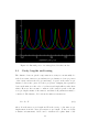
resonance frequencies for a given cavity. Figure 2.7 shows a plot of Equation
2.3 for modes 00 (red), 10 (green), and 20 (blue). Note that two modes can
be resonant at the same frequency if their phase shifts are the same.
12
Figure 2.7: Internal power of a cavity plotted for three modes.
2.3
Cavity lengths and tuning
The distance between optical components in a cavity is conventionally described as a sum of macroscopic and microscopic distances. Some properties
of the cavity, such as the free spectral range, depend on the macroscopic
distance between the optics. For those properites, changing the separation
between the mirrors on the order of one laser wavelength will not affect their
values. However, the resonance condition of the cavity depends on the microscopic displacements of the mirrors, and thus both parameters must be
considered. The distance, 𝐷, between the mirrors is written as
𝐷 =𝐿+𝑇
(2.8)
where 𝐿 is the macroscopic length and 𝑇 is the tuning, or the microscopic
displacement from the exact given macroscopic length. 𝑇 here is clearly
a distance measurement, but it can be rewritten as a phase shift of the
13
Gaussian beam. We will call this phase shift, governed by the microscopic
tuning, Δ𝑥 ([3]).
Now, Figure 2.5 plots the internal power of the cavity against frequency.
It shows, for example, that the cavity is resonant at the frequencies that
correspond to the peaks in the graph. Note that Figure 2.7 plots the internal
power against Δ𝑥, a value expressed in degrees. These are the same graphs
but plotted as functions of different (equivalent) variables. The difference
lies in rewriting the argument of the cosine term from Equation 2.3 with Δ𝑥
instead of 2𝑘𝐿. Δ𝑥 is expressed as an angle measurement, where 2𝜋 radians
(or 360∘ ) corresponds to a displacement of the mirror by one wavelength.
We have chosen to plot over Δ𝑥 instead of 𝑓 because we are assuming a
system with a fixed laser frequency and a tunable mirror displacement.
2.4
Behavior of a cavity
For the moment, we are interested in the resonant properties of a cavity
as it affects the internal power of the cavity and the transmitted power
(through the second mirror). This behavior for a two-mirror cavity depends
on the length of the cavity and on the reflectivities of the mirrors. There
are, then, three different cases that can govern this behavior. If 𝑇1 < 𝑇2 ,
the cavity is undercoupled. If 𝑇1 = 𝑇2 , the cavity is impedance matched. If
𝑇1 > 𝑇2 , the cavity is overcoupled. (Note that these can be rewritten as: If
𝑅1 > 𝑅2 , the cavity is undercoupled ; if 𝑅1 < 𝑅2 , the cavity is overcoupled.)
An undercoupled cavity will transmit little power through mirror 2 and
will not have much circulating power. An overcoupled cavity will have the
greatest circulating power and other internal resonance conditions. However,
an impedance-matched cavity maximizes the power transmission, and it is
the only condition under which the cavity can transmit (on resonance) one
hundred percent of the input power ([3]).
14
Chapter 3
The Optical Resonator
Calculator
3.1
Optical Resonator Calculator - The Idea
It was our goal to express some of the equations and properties of optical
cavities (as described in Chapter 2) visually. A graphical representation
can often teach much more about an equation’s properties than doing the
calculations by hand. It can give a student (or researcher) a more intuitive understanding of what the equation actually means in a physical sense.
Therefore, with the background knowledge about the physics of optical systems, we hope to create a useful visual tool (and reusable code) to simulate
the properties discussed above as they pertain to gravitational wave detector
interferometers.
For our first version of the calculator, we chose to model the internal power
of a two-mirror optical cavity as a function of the tuning. The cavity being
modeled consists of one flat mirror and one spherical mirror. It is important
to model the internal power because it shows, graphically, the tuning values
for which the cavity is resonant or anti-resonant. We wanted to plot the
internal power for three different transverse modes: 𝑇 𝐸𝑀00 , 𝑇 𝐸𝑀10 , and
𝑇 𝐸𝑀20 . Also, we thought it would be interesting to visually depict the
output power of the cavity at a user-defined value for tuning. We gave the
user the ability to control, via simple sliders and text fields, the reflectivities
15
of each mirror, the radius of curvature of the second mirror, and the value of
Δ𝑥 (the tuning). With this setup, this version of the calculator should help
users to visualize the internal power function, the Guoy phase, the power
output, the FSR, and the overall phase shift of a beam. Also, it should depict
how changing the reflectivities or radii of curvature of a cavity’s mirrors
affects the beam inside the cavity.
3.2
Project Overview
The Processing IDE which we chose to use for our program already had
code libraries for simple GUI components. For example, it provides code for
check boxes, text fields, buttons, and some other components. However, it
had very little or no libraries pertaining to sliders, meters, or graphs. Our
first task, then, was to write extendable libraries for the components we
needed. Each student in our group had a different main project, but each
of us wrote some library functions that could be used by all of us (and by
others). I will focus only on the small pieces that are directly used in the
Optical Resonator Calculator. One student in our group, Daniel Brown,
wrote the library for, among many other things, the sliders. Charlotte Bond
wrote the code for the LEDMeter, the meter which is used in this case to
show the cavity’s transmitted power.
I, then, wrote a two-dimensional plotting library. This plotting library allows
a user to plot many traces and many separate graphs. It can plot any
two-dimensional function. Other (and probably better) plotting libraries
exist in Java or Processing, but it was an integral part of my education in
programming to write a plotting library from scratch. Rather than simply
using a pre-made library, I designed my own as an exercise in becoming more
familiar with the language and object-oriented programming.
All three of these libraries were designed to be very general so they could
be incorporated into various programs. I will not go into further detail here
about how these libraries work because it is all explained in the actual code.
The code for the optical resonator calculator, which uses these libraries, is
included in Appendix A. This should give a more complete picture of how the
various libraries and components are linked to create the Optical Resonator
Calculator.
16
3.3
The User’s Manual
The Optical Resonator Calculator program has been uploaded to the project’s
webpage as a Java applet with some explantory text. This Java applet models some features of an optical resonator (also known as an optical cavity)
using a graphical user interface (GUI). The GUI allows a user to change
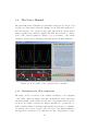
some of the cavity’s parameters. Figure 3.1 is a screenshot of the actual
calculator. Please refer to this image throughout the following discussion.
Figure 3.1: A screenshot of the optical resonator calculator.
3.3.1
Introducing the GUI components
The image on the bottom left of the calculator in Figure 3.1 is a diagram
of the cavity. This very simple cavity has essentially the same basic setup
and functionality as the cavities in each arm of a gravitational wave interferometer. It consists of a laser, two mirrors (in this case, one flat and one
with a variable radius of curvature) with variable reflectivites, a beamsplitter with two photodetectors, and a photodetector for the light transmitted
through the second mirror. Note that there are three sliders and accompa17
nying text fields overlaying the cavity image. The bottom left slider controls
the reflectivity of the first mirror, while the bottom right slider controls the
reflectivity of the second (rightmost) mirror. These reflectivities can range
from 0.00 to 0.99, as one cannot have a mirror with a perfect reflectivity of
1.00. These will be referred to, respectively, as the “𝑅1 slider” and the “𝑅2
slider.” (Likewise, the left mirror is mirror 1, and the right mirror is mirror
2.) The remaining slider above these controls the inverse of the radius of
curvature of the second mirror, and will commonly be referred to as the
“RoC slider.”
The graph above the cavity schematic is the graph of the logarithm of the
cavity’s internal power as a function of the microscopic tuning of the second
mirror. The logarithm of the internal power is plotted for three different
transverse modes: 𝑇 𝐸𝑀00 in red, 𝑇 𝐸𝑀10 in green, and 𝑇 𝐸𝑀20 in blue.
(The use of the logarithmic scaling will be explained later.) The tuning is
measured in degrees, where 360∘ is a microscopic displacement of the second
mirror by one wavelength. Below the graph, there is a slider (called the “Δ𝑥
slider”), which can be placed anywhere along the x axis. By default, this
slider has a white line attached to it that indicates precisely where the slider
is lining up with the plots above.
Finally, the meter on the bottom right of the calculator below the text box
indicates the percentage of the input power that is outputted through the
second mirror (reaching the rightmost photodetector). We will call this
meter the “transmitted power meter,” or simply “the meter.” This meter is
linked to the Δ𝑥 slider, so it shows the total power output for the tuning
value given by the Δ𝑥 slider.
3.3.2
The mathematical details
This calculator is essentially only using two equations. It is graphing the
base-10 logarithm of the internal power function given in Chapter 2 by Equation 2.3. The actual function being plotted, then, is
𝑙𝑜𝑔(𝑃1 ) = 𝑙𝑜𝑔(
𝑇1
),
1 + 𝑅1 𝑅2 − 2𝑟1 𝑟2 𝑐𝑜𝑠(2𝑘𝐿 + 𝜓𝑟𝑡 (𝑛 + 𝑚 + 1))
18
(3.1)
where, 𝜓𝑟𝑡 is the Guoy phase given by Equation 2.7. Then, the calculator
computes the transmitted (output) power of the cavity by adding, at the
chosen value of Δ𝑥, the internal power functions for each mode and multiplying the sum by the transmission coefficient of the second mirror. Since
𝑅2 + 𝑇2 = 1, this coefficient is simply given by
𝑇2 = 1 − 𝑅2
(3.2)
where 𝑅2 is controlled by the 𝑅2 slider. Therefore, for a given beam with
1 W of input power and mode 𝑇 𝐸𝑀𝑛𝑚 , the transmitted power, 𝑃𝑡𝑟𝑎𝑛𝑠 , is
calculated as
𝑃𝑡𝑟𝑎𝑛𝑠 = 10𝑙𝑜𝑔(𝑃1 ) ⋅ 𝑇2
(3.3)
In the cavity used in this calculator, there are three beams (three different
transverse modes). Each beam, for the sake of overall simplicity, has an
input power of 31 𝑊 , so that the total input power for the cavity is 1 𝑊 .
Therefore, the maximum amount of power that can be transmitted through
the second mirror is 1 𝑊 , as shown on the transmitted power meter. (As
explained in Chapter 2, this can only occur in an impedence-matched cavity.)
It is convenient for the transmitted power meter to range in value from 0
to 1 because it can then be thought of as representing the percentage of the
input power that is being transmitted (e.g. a value of 0.89 is 89% of the
input power).
To improve the appearance of the plot of the cavity’s internal power, it is
typically graphed on a logarithmic scale. This is done because the peaks
in the plot on a normal scale become extremely sharp, especially for highly
reflective mirrors. Plotting on a logarithmic scale smooths out the graph
a little bit. When you look at the calculator’s graph, you may wonder
why we are plotting the logarithm of the power, rather than plotting the
power on a logarithmic scale. We chose to do this because having axes with
evenly-spaced tick marks is much more compatible with the two-dimensional
plotting function that I wrote than having axes on a logarithmic scale. When
viewing the graph, the user still has the ability to see what value the power
has, and it does not make the calculations much more difficult.
19
3.3.3
How to use the GUI controls
The controls have been designed to be as simple as possible to use. Each
slider can be controlled by the mouse by either clicking or dragging the slider
to its desired position. Also, if you set the program’s focus to a particular
slider by clicking on it, that slider can then be moved by one pixel at a time
using the left and right arrow keys. This helps mostly for the Δ𝑥 slider
when trying to choose a precise tuning value.
When the slider value is changed in this way, the associated text field changes
to the chosen slider value. Additionally, the slider value can be changed by
directly typing the desired value into the text field and then hitting the
‘Enter’ key. Note that if ‘Enter’ is not pressed, the slider will not update
to that value. The 𝑅1 , 𝑅2 , and Δ𝑥 sliders all have a maximum precision of
two decimal places. If you type in a value of, say, 0.487, the slider should
round this number to 0.49. However, it is best if at most two decimal places
are used so unexpected rounding does not occur.
Finally, please note that the RoC slider actually controls the inverse of the
radius of curvature of the second mirror. That is, the value represented by
1
. This is done so the radius of curvature can
the RoC slider is actually 𝑅𝑜𝐶
range from 𝐿 (the cavity length, 1 m) to infinity (a flat mirror). Infinity cannot be represented by a slider, but 1/𝑖𝑛𝑓 𝑖𝑛𝑖𝑡𝑦 is essentially zero. Therefore,
the RoC slider ranges from 0.0 (for an infinite radius of curvature) to 1.0
(for a radius of curvature equal to the cavity length of 1 m).
The Δ𝑥 slider does not have a text field, and it does not display its current
value. The value is represented by the corresponding tick marks on the x
axis of the graph. By default, this slider has a white line linked to it which
helps to see where on the graph the slider is positioned. This line can be
switched off, though, by unselecting the check box to the right of the graph
labelled “Show white line for delta x.”
3.3.4
Configurations to try
In most optical resonators, highly reflective mirrors are used to enhance the
power within the resonator. This is true for gravitational wave interferometers. If you set the 𝑅1 and 𝑅2 sliders to 0.99 reflectivity, you will see that
20
the peaks in the internal power plot become very sharp. Equation 3.3 shows
that the transmitted power is proportional to 𝑇2 . When 𝑅2 is very close to
1.00, 𝑇2 becomes very small. Therefore, the internal power is only large for
resonance conditions. This makes the precise tuning of the cavity extremely
important if one is to achieve resonance.
The calculator will also allow you to visualize the differences among undercoupled, overcoupled, and impedance-matched cavities. These configurations were described in detail in Chapter 2. The calculator’s default is an
impedance-matched cavity with high reflectivities (𝑅1 = 𝑅2 = 0.96). This
is the only condition under which, on resonance, the cavity can transmit all
of the input power (in this case, 1 W). Altering the radius of curvature of
the second mirror (using the RoC slider) changes the Rayleigh range (𝑧𝑅 )
of the beam and therefore the round-trip Guoy phase (see Equation 2.7).
In particular, the larger the radius of curvature (as 1/𝑅𝑜𝐶 approaches 0),
the smaller the Guoy phase shift. This is why as you decrease 1/𝑅𝑜𝐶, the
peaks of the internal power for the different modes become very close and
eventually overlap. At an infinite radius of curvature, the Guoy phase shift
is 0, and multiplying the phase shift by (𝑛 + 𝑚 + 1) (as in Equation 2.3) will
not change the overall phase shift for different modes.
An undercoupled cavity is one in which 𝑇1 is less than 𝑇2 , so 𝑅1 is greater
than 𝑅2 . This type of cavity has little circulating power. If you set the
𝑅1 slider to be greater than the 𝑅2 slider, you can notice that the internal
power becomes small, and even on resonance there is very little transmitted
power (compared to an impedance-matched cavity).
An overcoupled cavity is one in which 𝑅1 is less than 𝑅2 . It has a high
circulating power compared to an impedence-matched cavity which has reflectivities equal to the lower reflectivity in the overcoupled cavity. However,
with 𝑅2 high, 𝑇2 is low and there is little transmitted power.
These are some of the simple cavity properties that this calculator illustrates.
At the very least, it should give users a more intuitive sense about how the
cavity parameters affect its resonance properties. It is probably most useful
if one views the circulating (internal) power function (Equation 2.3) while
running the program to see how the plots are being affected.
21
3.3.5
Intentional limitations
In the first and current version of this calculator, the user only has limited
control over the cavity’s parameters. Only four parameters can actually be
set by the user: the reflectivity of the first mirror, the reflectivity of the
second mirror, the radius of curvature of the second mirror, and the tuning
of the cavity. Giving the user many more values to change would make it
more difficult for the user to really learn a few basic concepts about cavities
and could be confusing. We wanted to make this version simple so that it
would illustrate only a few key points. Therefore, the user cannot change
parameters such as the configuration of the cavity, the cavity length, the
curvature of the first mirror, the beam modes, etc. We felt that this would
be too much information to include in an educational or reference tool,
though it probably would not be very difficult to include in future versions.
Also, this applet is not quite a calculator in the usual sense of the word. In
a usual calculator, one would enter some values and get precise numerical
answers in return. While this is certainly useful, outputting exact numbers is
not necessarily useful when simply portraying relations between parameters.
It may also become overwhelming or confusing for a student using the tool
if many numbers are outputted to the screen. Again, though, numerical
output could be easily included in future versions of the calculator if so
desired.
22
Chapter 4
Bugs and Future Directions
4.1
Remaining Problems and Bugs
There are only a few remaining problems with the current version of the
Optical Resonator Calculator. These are described in detail below. For the
more code-involved problems, it would probably help to know how the actual
code works (in the libraries and the source code included in Appendix A).
However, the explanations of the problems below should not require much
prior knowledge of the code.
The most notable bug can be seen when the reflectivities of the mirrors are
very high (≳ 0.97). In this case, it is difficult to align the Δ𝑥 slider with
the peaks precisely, and the transmitted power meter does not quite display
the correct value. For instance, if 𝑅1 = 𝑅2 = 0.99 and 1/𝑅𝑜𝐶 = 0.5, if
the cavity is on resonance, the meter should read, for each beam mode, a
transmitted power of 31 W. The value it actually shows is closer to 0.1 W.
This bug is probably due to an inherent resolution issue with the graphical
output. To increase the resolution around sharp peaks, the two-dimensional
plotting function implements a loop which is not also implemented exactly
by the transmitted power meter calculations. In this loop, for each pixel
along the x axis, the plotting function converts the pixel number into graph
units, takes six points in graph units between each pixel, calculates the y
value for each of these points (in graph units), and finally chooses to plot
the maximum of these as the y value corresponding to the original x pixel.
23
For various detailed reasons having to do with object-passing and private
variables, this same loop is not easy to use for calculating the transmitted
power. Currently, the calculation for the transmitted power does not directly
’read’ the y values off of the graph. Instead, it computes the y value given
the value of the Δ𝑥 slider without the loop just described. Therefore, I
believe the values being plotted are not quite the same values computed at
the precise value of the Δ𝑥 slider. This may cause the slight discrepancy for
sharp peaks. This may not be the actual reason, though. This bug was not
resolved after several attempts and adjustments and therefore has been left
for future revisions.
The remaining problems are not necessarily bugs but rather improvements
that should probably be made to the code. Currently, the program (or
’sketch’ as it is called in Processing) invokes a lot of processing time from the
computer running it. In Processing sketches, there are two main functions:
setup and draw. The setup function is meant to contain all the object and
variable declarations, initializations, and other fixed parameters. It only
runs once when the sketch runs. The draw function, however, is meant to
react to changes made while the sketch is running (such as moving a slider).
Therefore, it runs many times to update the graphics. In this sketch, this
and the functions doing the calculations seem to be consuming a lot of
processing power. Slight code variations should be implemented to reduce
this problem. For example, telling the draw function to run only if some
’event’ has actually occurred. Other modifications could be made to make
the sketch more efficient.
Finally, due to my relative lack of experience in programming, there are
some limitations in the two-dimensional plotting class. It is quite sensitive
to the precise numbers being use for, say, the axis length and the tick mark
spacing. This issue is described in the comments of this code, but it should
be highlighted here as well. In order for the scaling between the pixels
and the graph units to be accurate when calculating the actual plot, one
must be very sure that the axis length is an exact multiple of the spacing
between the tick marks. If this is not quite possible, the plots may be
slightly inaccurate. Now, the spacing between the slider’s tick marks is, on
the other hand, calculated by dividing the axis length by the number of tick
marks the user wants on the slider. This can lead to small rounding issues
because pixels must be represented as integers. If the quotient done in this
24
calculation is not exactly an integer, the quotient is rounded or truncated.
In the Optical Resonator Calculator, the x axis of the graph is supposed
to be precisely linked with the Δ𝑥 slider. Because of this difference in the
coding of these two components, one has to be very careful (and very precise)
about the values chosen for each. There does not seem to be a problem in
this program, but if modifications are made, this conflict must be taken into
account.
4.2
Possible Future Directions
One of the main purposes of this project was to establish a foundation for
possible future simulations for gravitational wave detector optics. A large
amount of the time was spent writing library codes in the hope that they
would be used in other projects. The simulations created, like the Optical
Resonator Calculator, were intended to be used on the Internet but also to
show other people what can be done with the library code.
This calculator is simply the first version created of what could be a series of
different simulation programs/applets. With this in mind, some suggestions
have been compiled for possible newer versions of the calculator:
ˆ Output some numerical values given the slider or text field input
ˆ Allow adjustments to more parameters (cavity length, beam modes,
input power, mirror 1 radius of curvature, cavity configuration, etc.)
ˆ Output an image of the beam shape
ˆ Calculate waist size of the beam at a chosen point
These are by no means all the possible things that could be implemented or
useful, but some would probably be a good starting point. We hope that
the simulations will remain self-consistent and simple, portraying only a few
concepts in each simulation.
With the foundational projects the students working with Dr. Andreas
Freise at the University of Birmingham have done this summer, more simulations and educational and research tools should begin to be created for
gravitational wave detector optics. For additional information concerning
the projects done this summer, please refer to
25
www.gwoptics.org/processing/
Also, more details about the source code can be found in Appendix A,
complete with all comments.
26
Appendix A
Appendix A
This is the exact Processing source code (as of 7 August 2009) being used for
the main file of the optical resonator calculator. It uses quite a few libraries
(as listed at the top of the code), and it also uses the classes Axis, AxisConfig, GraphCallback, LEDMeter, LEDMeterAxis, PlotAreaBackground,
PlotConfig, Plotting, and TraceConfig. This source code may be slightly
modified for the final version to be posted online, but the changes will only
be minor alterations. The final version’s source code and libraries will be
posted online also. For more detail about these classes, one must refer to
the code files for them, which are not included in this report for the sake of
brevity.
import
import
import
import
import
import
org.gwoptics.gui.slider.*;
org.gwoptics.ValueType;
guicomponents.*;
org.gwoptics.Logo;
org.gwoptics.LogoSize;
guicomponents.GCheckbox;
//declare variables, objects, and fonts
gwSlider R1slider;
GTextField R1textfield;
gwSlider R2slider;
GTextField R2textfield;
27
gwSlider RoCslider;
GTextField RoCtextfield;
gwSlider delta_x_slider;
LEDMeter meter;
LEDMeterAxis meterAxis;
AxisConfig axisconfig;
PlotConfig plotconfig;
TraceConfig traceConfig1, traceConfig2, traceConfig3;
PlotAreaBackground area1;
Axis xaxis,yaxis;
Plotting alltraces;
InternalPower00 mode00;
InternalPower10 mode10;
InternalPower20 mode20;
PFont font;
float R1,R2,delta_x,L,RoC;
PImage cavityimage;
Logo _logo;
PFont titleFont;
PFont expFont;
PFont meterTitleFont;
String explanationtext;
GCheckbox chkWhiteLine;
void setup()
{
size(900,600);
smooth();
L = 1;
//length of the cavity is fixed to 1 meter
//initialize the axis, plot, and trace config objects
axisconfig = new AxisConfig();
28
plotconfig =
traceConfig1
traceConfig2
traceConfig3
new PlotConfig();
= new TraceConfig();
= new TraceConfig();
= new TraceConfig();
//set the config settings
plotconfig.bordercolor = color(255);
plotconfig.fillcolor = color(0);
plotconfig.borderweight = 3;
axisconfig.axiscolor = color(255);
axisconfig.textcolor = color(255);
axisconfig.tickcolor = color(255);
traceConfig1.tracecolor = color(255,0,0); //each trace has its own
traceConfig1.traceweight = 2; //color so its own config object
traceConfig2.tracecolor = color(0,255,0);
traceConfig2.traceweight = 2;
traceConfig3.tracecolor = color(0,0,255);
traceConfig3.traceweight = 2;
//Initialize the Axes and PlotAreaBackground
//x pos, y pos, width, height, config object
area1 = new PlotAreaBackground(5,15,540,389,plotconfig.getConfig());
//x1,y1,x2,y2,axis label, config, axis zero
xaxis = new Axis(60,350,526,350,"delta x (degrees)",
axisconfig.getConfig(),293);
yaxis = new Axis(60,25,60,350,"log of Intensity",
axisconfig.getConfig(),188);
//Tick label formatting
xaxis.setTickLblFormat("%.0f");
//no decimal places for the ticks
//(length of x axis in pixels)/(its length in graph space)
//= 33.28571429px/graph unit
xaxis.setMajorSpacing(33);
yaxis.setMajorSpacing(54);
//major tick labels start @ 0 and increment by 90
xaxis.setMajorLabels(0,90);
29
//major tick labels start @ 0 and increment by 1
yaxis.setMajorLabels(0,1);
xaxis.isZeroTickDrawn(true);
yaxis.isZeroTickDrawn(true);
//Axis label text formatting
xaxis.setTextPosition(300,400);
yaxis.setTextPosition(25,200);
//Initialize the trace objects
//need to pass the alltraces object the axes to be drawn on
alltraces = new Plotting(xaxis,yaxis);
//these are the internal power equations being used, one for each mode.
mode00 = new InternalPower00();
mode10 = new InternalPower10();
mode20 = new InternalPower20();
//tell alltraces which traces and configs you want
alltraces.addTrace(mode00,traceConfig1);
alltraces.addTrace(mode10,traceConfig2);
alltraces.addTrace(mode20,traceConfig3);
//Initialize and add all the sliders
R1slider = new gwSlider(this,200,559,110);
R1slider.setTickColour(255,255,255);
R1slider.setFontColour(255,255,255);
R1slider.setValueType(ValueType.DECIMAL);
//1.00 reflectivity is unrealistic, so we set the limit to 0.99
R1slider.setLimits(0.96,0.00,0.99);
R1slider.setTickCount(5);
R1slider.setPrecision(2);
//This sets the textfield value for before you move the slider.
R1textfield = new GTextField(this,String.valueOf(0.96),160,557,36,15);
R2slider = new gwSlider(this,370,559,110);
R2slider.setTickColour(255,255,255);
30
R2slider.setFontColour(255,255,255);
R2slider.setValueType(ValueType.DECIMAL);
R2slider.setLimits(0.96,0,0.99);
R2slider.setTickCount(5);
R2slider.setPrecision(2);
R2textfield = new GTextField(this,String.valueOf(0.96f),332,557,36,15);
RoCslider = new gwSlider(this,370,452,110);
RoCslider.setTickColour(255,255,255);
RoCslider.setFontColour(255,255,255);
RoCslider.setValueType(ValueType.DECIMAL);
//represents 1/RoC, so the RoC can range from L to infinity
RoCslider.setLimits(0.5,0,1);
RoCslider.setTickCount(5);
RoCslider.setPrecision(2);
RoCtextfield = new GTextField(this,String.valueOf(0.50f),332,450,36,15);
//doesn’t exactly line up with axis but close
delta_x_slider = new gwSlider(this,54,368,478);
delta_x_slider.setTickColour(255,255,255);
//default position for slider, min value, max value
delta_x_slider.setLimits(0,-3.5*PI,3.5*PI);
delta_x_slider.setTickCount(13);
delta_x_slider.setValueType(ValueType.DECIMAL);
delta_x_slider.setPrecision(2);
delta_x_slider.setRenderMaxMinLabel(false);
delta_x_slider.setRenderValueLabel(false);
//x,y,length,num,height,min,max
meter = new LEDMeter(557,490,349,30,20,0.0,1.0);
meter.setGradient();
meter.setGapSize(0);
//xpos, ypos, num labels, xstep, min, max
meterAxis = new LEDMeterAxis(557,500,10,33,0,1);
meterAxis.setFontSize(12);
31
//Importing images
cavityimage = loadImage("cavitypng.png");
_logo = new Logo(this, 770,570,true,LogoSize.Size25);
//Create fonts
titleFont = createFont("verdana",20);
meterTitleFont = createFont("verdana",13);
expFont = createFont("verdana",11);
//Write the explanation here
explanationtext = "This applet graphs the internal power of an optical "+
"cavity as a function of tuning for transverse modes 00 (red), 10 "+
"(green), and 20 (blue)."+
"The slider below the graph controls the tuning of the second mirror. "+
"Below, the meter shows the percentage of the input power that is "+
"outputted through the second mirror at the current value of delta x "+
"(the tuning). The cavity is drawn below the graph. Each mirror has "+
"a reflectivity slider. The 1/RoC slider controls the inverse "+
"of the Radius of Curvature of the second mirror. 1/RoC=0 represents "+
"a flat mirror (infinite RoC), and 1/RoC=1=L represents a radius of "+
"curvature equal to the length of the cavity (1m). "+
"Using the sliders, you should be able to notice changes in the "+
"Guoy phase and the FSR for the different modes. The sliders "+
"can be controlled with the mouse or left/right arrow keys.";
//Adds a checkbox to select whether or not we want the white line
//on the delta_x slider to show. Defaulted to yes/true
chkWhiteLine = new GCheckbox(this,"Show white line for delta x",
550,380,200);
chkWhiteLine.setSelected(true);
}
void draw()
{
background(200,200,200);
32
//Draw plotting area and the traces
area1.drawRect();
xaxis.drawAxis();
yaxis.drawAxis();
xaxis.drawMajorTicks();
yaxis.drawMajorTicks();
xaxis.drawMajorTickLabels();
yaxis.drawMajorTickLabels();
//need to know the x and y axis ranges in graph space
alltraces.plotTraces(-3.5*PI,3.5*PI,-3,3);
//Draw the cavity image
image(cavityimage,10,412);
//Assign the slider values to variables
R1 = R1slider.getValuef();
R2 = R2slider.getValuef();
delta_x = delta_x_slider.getValuef();
RoC = 1/(RoCslider.getValuef());
//Set and write the Title to the screen
textFont(titleFont);
fill(0);
text("Optical Resonator Calculator",720,30);
//Set and write a label for the meter
textFont(meterTitleFont);
fill(0);
text("Percent of Input Power Transmitted",720,480);
//Explanation box
stroke(255);
fill(190,204,223);
rect(575,45,300,328);
textFont(expFont);
fill(0);
33
text(explanationtext,579,49,295,340);
//Add logo
_logo.draw();
//Power meter. Apparently in Processing log is natural log... Also now
//each beam has an input power of 1/3 W, so the total input power is 1W.
float sum_delta_x = (pow(10,mode00.computePoint(delta_x))
+pow(10,mode10.computePoint(delta_x))
+pow(10,mode20.computePoint(delta_x)))/3;
float transmitted_power = sum_delta_x*(1-R2);
meter.setValue(transmitted_power);
meter.response();
meterAxis.display();
//Adjusting the line drawn off the slider for rounding errors
if(chkWhiteLine.isSelected()){
line((delta_x_slider.getValuef()*float(478/22))+293,368,
(delta_x_slider.getValuef()*float(478/22))+293,15);
}
}
//These are the functions that are being plotted. All the same except
//for different values of n
class InternalPower00 implements GraphCallback
{
int n,m;
float Power00;
float zR, psiRT;
public float computePoint(float t_delta_x)
{
delta_x = t_delta_x;
n = 0;
m = 0;
zR = sqrt(L*(RoC-L));
psiRT = 2*atan(L/zR);
34
//Need to convert the natural log to log base 10...
Power00 = log((1-R1)/(1+(R1*R2)-(2*sqrt(R1)*sqrt(R2)
*cos(delta_x+(psiRT*(n+m+1))))))/log(10);
return Power00;
}
}
class InternalPower10 implements GraphCallback
{
int n,m;
float Power10;
float zR, psiRT;
public float computePoint(float t_delta_x)
{
delta_x = t_delta_x;
n = 1;
m = 0;
zR = sqrt(L*(RoC-L));
psiRT = 2*atan(L/zR);
Power10 = (log((1-R1)/(1+(R1*R2)-(2*sqrt(R1)*sqrt(R2)
*cos(delta_x+(psiRT*(n+m+1)))))))/log(10);
return Power10;
}
}
class InternalPower20 implements GraphCallback
{
int n,m;
float Power20;
float zR, psiRT;
public float computePoint(float t_delta_x)
{
delta_x = t_delta_x;
n = 2;
m = 0;
zR = sqrt(L*(RoC-L));
35
psiRT = 2*atan(L/zR);
Power20 = (log((1-R1)/(1+(R1*R2)-(2*sqrt(R1)*sqrt(R2)
*cos(delta_x+(psiRT*(n+m+1)))))))/log(10);
return Power20;
}
}
//This method tells the prorgam what to do if the user
//moves the sliders
void handleSliderEvents(gwSlider slider){
float precision = 100;
if(slider == R1slider){
R1textfield.setText(String.format("%.2f",slider.getValuef()));
}
if(slider == R2slider){
R2textfield.setText(String.format("%.2f",slider.getValuef()));
}
if(slider == RoCslider){
RoCtextfield.setText(String.format("%.2f",slider.getValuef()));
}
}
//This method tells the program what to do if the user types a
//value into a textfield and hits ’Enter’
void handleTextFieldEvents(GTextField tfield){
String line1="";
float temp_val;
if(tfield == R1textfield){
switch (R1textfield.eventType){
case GTextField.CHANGED:
break;
case GTextField.SET:
break;
case GTextField.ENTERED:
line1=R1textfield.getText();
temp_val = parseFloat(line1);
36
R1slider.setValue(temp_val);
break;
}
}
if(tfield == R2textfield){
switch (R2textfield.eventType){
case GTextField.CHANGED:
break;
case GTextField.SET:
break;
case GTextField.ENTERED:
line1=R2textfield.getText();
temp_val = parseFloat(line1);
R2slider.setValue(temp_val);
break;
}
}
if(tfield == RoCtextfield){
switch (RoCtextfield.eventType){
case GTextField.CHANGED:
break;
case GTextField.SET:
break;
case GTextField.ENTERED:
line1=RoCtextfield.getText();
temp_val = parseFloat(line1);
RoCslider.setValue(temp_val);
break;
}
}
}
37
*Acknowledgements
I would like to thank everyone at the University of Birmingham and the University of Florida’s IREU for their help with this project and my scientific
learning this summer. In particular, my thanks go to my project supervisor,
Dr. Andreas Freise, for all his patience and organization with the summer
projects; to all the people in Andreas’s group: Dr. Stefan Hild, Dr. Simon
Chelkowski, Paul Fulda, Antonio Perreca, Jonathan Hallam, Deepali Lodhia, and Keiko Kokeyama, for always being available to help; to the other
summer students (Charlotte Bond, Emil Schreiber, and Matthew Arnold)
for helping so much to make this project successful (particularly Charlotte,
who contributed code for the Optical Resonator Calculator); and to Daniel
Brown, another summer student, who contributed extensive amount of code
and libraries to this project and was my go-to person for most of my programming questions. I’d also like to acknowledge Professor Bernard Whiting, Professor Guido Mueller, and all others involved with this program
at the University of Florida for all their work with the International REU
program. Last but not least, my gratitude goes to the National Science
Foundation (NSF) for funding and supporting the REU program.
38
Bibliography
[1] Ben Fry and Casey Reas. Processing. Website, 2009. http://www.
processing.org.
[2] Antonio Perreca. Lecture Notes. Summer lecture notes, University of
Birmingham, July 2009.
[3] Dr. Andreas Freise. Lasers and Quantum Optics. Year 4 Lecture Notes,
University of Birmingham, April 2009.
39
40