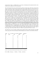
Download fulltext01 - DiVA Portal

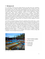
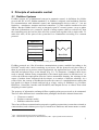
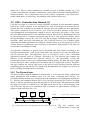
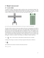
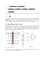
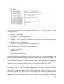
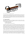
UPTEC F10 040
Examensarbete 30 hp
Juli 2010
Controller programming with
CoDeSys for an automated timber
sorting system
Nils Breitholtz
Abstract
Controller programming with CoDeSys for an
automated timber sorting system
Nils Breitholtz
Teknisk- naturvetenskaplig fakultet
UTH-enheten
Besöksadress:
Ångströmlaboratoriet
Lägerhyddsvägen 1
Hus 4, Plan 0
Postadress:
Box 536
751 21 Uppsala
Telefon:
018 – 471 30 03
Telefax:
018 – 471 30 00
Hemsida:
http://www.teknat.uu.se/student
This report describes the development of weight measurement application and
transducer positioning for the A Sort prototype that has been developed for
automatic grading and sorting of timber. The prototype consists of a transportation
system with hydraulic and electrical motors, a measurement system with laser
scanners and acoustic measurement equipment and a control program for the
automated process with CoDeSys. The objective was to integrate these parts in an
automatic system process, controlling a prototype designed for acoustic measurement
of logs. The devices were installed and configured to communicate via an existing
fieldbus line using CANopen as communication protocol. A control program was
made for each task and implemented in the control process for the automatic
measurement of logs. Two load cells were installed beneath a moving tilt and the
measurement equipment was tested and calibrated using three different logs with
known weight. The testing showed that in order to get higher accuracy the
construction needs to be modified. Photo cells were installed on the measurement
frames and a program was made in order to make the acoustic measurement of the
logs work properly.
Handledare: Christer Karlsson
Ämnesgranskare: Ping Wu
Examinator: Tomas Nyberg
ISSN: 1401-5757, UPTEC F10 040
1
BACKGROUND.......................................................................................................................................... 4
2
PRINCIPLE OF AUTOMATIC CONTROL ........................................................................................... 5
2.1
2.2
2.2.1
2.2.2
2.2.3
2.3
2.4
2.5
3
THE PROTOTYPE................................................................................................................................... 12
3.1
3.2
3.3
3.3.1
3.3.2
3.3.3
3.3.4
3.3.5
3.3.6
3.4
4
FEATURES ........................................................................................................................................... 12
THE CONTROL PROGRAM .................................................................................................................... 13
LOG TRANSPORTATION ....................................................................................................................... 14
The conveyer in table – Conv_in(PRG)......................................................................................... 14
The step feeder – Step_feeder(PRG) ............................................................................................. 14
The roller conveyer – Roller_conv(PRG)...................................................................................... 15
The feeder wheel – Feeder_wheel(PRG)....................................................................................... 15
The tilt – Tilt(PRG) ....................................................................................................................... 15
The conveyer out table – Conv_out(PRG)..................................................................................... 15
THE HYDRAULIC SYSTEM .................................................................................................................... 15
WEIGHT MEASUREMENT ................................................................................................................... 17
4.1
4.2
4.3
4.4
4.4.1
4.4.2
4.4.3
4.4.4
5
FIELDBUS SYSTEMS .............................................................................................................................. 5
CAN – CONTROLLER AREA NETWORK [1 ] .......................................................................................... 6
The Physical layer........................................................................................................................... 6
The Data Link layer......................................................................................................................... 7
Bus arbitration and error management........................................................................................... 8
THE APPLICATION LAYER – CANOPEN [4]............................................................................................ 8
PLC AND SOFTPLC ............................................................................................................................ 10
CODESYS – A PROGRAMMING ENVIRONMENT FOR PLC AND SOFTPLC ............................................. 10
LOAD CELLS[8] ................................................................................................................................... 17
COMMUNICATION WITH THE NODE...................................................................................................... 19
WEIGHT MEASUREMENT PROGRAM ..................................................................................................... 23
RESULTS ............................................................................................................................................. 25
Empty cradle ................................................................................................................................. 25
Result test 1: Log weight 116 kg ................................................................................................... 25
Result test 2: Log weight 181 kg ................................................................................................... 26
Result test 3: Log weight 225 kg ................................................................................................... 26
MEASUREMENT FRAME POSITIONING.......................................................................................... 29
5.1
5.2
IMPLEMENTATION ............................................................................................................................... 30
THE PROGRAM .................................................................................................................................... 32
6
CONCLUSIONS AND SUGGESTIONS FOR FUTURE WORK ........................................................ 36
7
REFERENCES .......................................................................................................................................... 37
1 Background
Use of automatic control has grown rapidly during the last century and is now a mandatory
part of our industry. As with the introduction of programmable logic controllers (PLCs) and
microcomputers in the late 1960s control engineering has become more related to electrical
and computer engineering. The implementation of fieldbus systems and industrial networking
in general has made it possible to coordinate a multiple of control applications, creating a
control system. These control applications could be, for example, motion control,
mathematical calculation processes, digital signal processing or pneumatic- and hydraulic
control, all ran or supervised by a single or a network of computers. Today’s market offers a
number of possible solutions regarding communication protocols, centralized or distributed
I/Os, program developing environments and system configuration in general, all depending on
different user demands. In order to determine which system products are best suited for an
application, a large number of aspects have to be taken into account, making the selection
process very demanding.
A Sort AB is currently developing a prototype for automatic sorting of timber (Fig. 1.1). The
idea is, by using acoustic measurement, to pre-sort timber before it goes into sawing mill. The
prototype is designed to transport a log through a system of different measuring devices to
gather information needed to determine the physical properties of the log. In order to do that
the sorting process needs to be controlled and coordinated in the aspects of the measurement
devices and the transportation of logs. The main purpose of this thesis is to determine the
mass of logs along with the development of a method for the positioning of measurement
equipment for the prototype. A main tool for this thesis project is CoDeSys (Controller
Development System) which is a comprehensive software tool for industrial automation
technology [3]. The fieldbus in use is controller area network (CAN) [6] along with
CANopen, a CAN-based application protocol [4].
Fig. 1.1 The A Sort prototype
4
2 Principle of automatic control
2.1 Fieldbus Systems
Fieldbus systems are a fundamental concept in automatic control. A definition for fieldbus
given in the IEC 611581 fieldbus standard is “A fieldbus is a digital, serial multidrop, data bus
for communication with industrial control and instrumentation devices such as – but not
limited to – transducers, actuators and local controllers.”[1] This could be considered as a bit
diffuse. But the fieldbus itself is only an integrative part of a control system, a way to gather
and share information over a network. Instead of using separate cables to each device from
the controlling unit, the bus line links all of the system parts together with a single cable. To
make this work, all the parts of the system have to communicate according to a common
protocol.
Application
Presentation
Session
Transport
Network
Application
Data Link
Physical
Data Link
Physical
Fig. 2.1 CAN according to the ISO/OSI model
Fieldbus protocols are, like all modern communication systems, modelled according to the
ISO/OSI2 model with a stack containing seven layers, but the protocols only have three of
them in practical use in process control applications: the application layer on the top and the
data link and physical layer at the bottom (Fig. 2.1). To determine a standard, these layers
need to interact without losing compatibility with control applications in different areas. As
well as the different requirements from the various automation domains, the winnings in the
aspect of market shares influenced the developers to a number of different solutions. As a
result of this, the concept of fieldbus has become the centre of a standardisation conflict that
has lasted over almost a decade and has left us a large variety of fieldbuses (e.g. Profibus,
PROFInet, ControlNet, Interbus and WorldFIP) and adapted devices to choose from when
designing a control system.
The property of information exchange differs regarding what process needs to be automated.
There are three different basic communication paradigms declared for industrial networks:
•
•
•
Client-server model
Producer-consumer model
Publisher-subscriber model
These have different communication properties regarding connections (connection oriented or
connectionless) and relations (peer to peer, broadcast or multicast; and mono-master or multi-
1
2
IEC – International Electrotechnical Commission.
ISO – International Organization for Standardization; OSI – Open Systems Interconnection.
5
master, etc.). They are often combined in a number of ways in fieldbus systems, e.g. CAN
(Control Area Network) is mainly a combination of the producer-consumer and the publishersubscriber model. Yet, it implements some of the features recognised as the client-server
model which makes, in some sense, this labelling a bit pointless in this case.
2.2 CAN – Controller Area Network [1 ]
CAN has its origin in a serial bus system originally developed for the automation industry
back in the 1980s by Bosch. It was intended to be used in passenger cars because the bus
systems that were available on the market at that time were not suitable for their application.
This system Automotive Serial Controller Area Network proved its qualities in the area of
error management and congestions, enough to survive and evolve into today’s CAN. From
this, two different solutions of CAN controllers surfaced: BasicCAN by Philips and FullCAN
by Intel. BasicCAN is a simpler version that only involves send and receive buffers where
message handling is run by the CPU. The CPU has to request or acknowledge the data via
interrupts, which will in the end burden the CPU. FullCAN involves a set of buffers called
mailboxes that handle information according to contents, where no involvement of the CPU is
needed. These two architectures have been more or less united, when modern CAN chips are
structured as a combination of both.
As told above fieldbuses in general can be modelled with three layers according to the
ISO/OSI standard model. CAN, on the other hand, only consists of two: the data link layer
and the physical layer. The application layer is covered by some of the CAN-based
application protocols such as CANopen, DeviceNet, etc. The physical layer handles the
function of the mechanical and electrical aspects, i.e., the connections, wiring and
transmission media as well as the synchronization and bit timing. The data link layer is split
into two sub layers: MAC (medium access control) and LLC (logical link control). The MAC
sub layer controls the activity and access to the bus to avoid collisions between different
transmitting devices whereas the LLC handles the bus arbitration on a higher level as well as
frame encoding, decoding and error checking.
2.2.1 The Physical layer
The most common physical medium for data transfer is a two-wire bus, using a differential
signal transmission with common return. The two wires, CAN-high and CAN-low, are
preferably shielded twisted pair, which increases the immunity to electromagnetic interference
[1]. There are two standards defined, ISO 11519 (CAN low speed) and ISO 11898 (CAN high
speed). CAN low speed has an upper bit rate limit of 125 kbit/s and CAN high speed is within
the range of 10 kbit/s to 1 Mbit/s. For CAN high speed (used in the A Sort prototype), each
end of the bus line has to be terminated with a resistance of approximately 120 Ω[5] to
suppress signal reflection (Fig. 2.2).
CAN
node 1
CAN
node 2
CAN
node 3
CAN_H
120 Ω
120 Ω
CAN_L
Signal
Recessive state
Dominant state
CAN HIGH
2.5 V
3.5 V
CAN LOW
2.5 V
1.5 V
Fig. 2.2 Description of the CAN high speed bus line and the signal levels
The bus assumes two
different states or levels and
6
since the outputs of the nodes connected to the bus are based on the principle of an opencollector it will work as a wired-AND. A wired-AND works like a Boolean AND, in this case
meaning that any node transmitting lower level output will result in a low bus level. The two
bus levels are referred to as dominant and recessive where the logical value of the dominant
level is 0 and the logical value of the recessive level is 1. CAN uses non-return to zero bit
encoding which basically means that there is no “neutral state” in between the bits. This
means that level on the bus will remain unchanged when transmitting a consecutive series of
values. Therefore, an additional synchronisation is needed to avoid errors, or “bit-slips”. By
using a digital phase-locked loop each node can extract the necessary bit-timing information
from the flanks in the bit stream[1]. And to ensure a decent level of synchronisation CAN
adds a sufficient number of flanks in the bit stream, by so-called bit-stuffing. Five bits of the
same logical value will be followed by an extra bit of the opposite value, and thereby adding
an extra flank in a consecutive bit stream. These extra bits are removed, or de-stuffed, by the
receiver.
2.2.2 The Data Link layer
CAN is a multi master network where a data frame is addressed with an identifier rather than
an actual node address. Here, CAN specification uses two types of frame formats, the
standard (CAN 2.0A) with an 11-bit identifier field (
Fig. 2.3) and the extended (CAN 2.0B) format with an extra 18-bit identifier field giving a
total of half a billion different objects in the same network. Modern systems are in most cases
capable of recognizing and adjusting to both formats but the standard CAN 2.0A is most
common and sufficient for almost any application.
11 bit
S
O IDENTIFIER
F
R I r
T D 0
R E
DLC
0-8 byte
DATA
FIELD
CRC
FIELD
ACK
FIELD
EOF
IMS
Fig. 2.3 The frame format in standard CAN
When the network is idle and no frames are being sent, the level on the bus is recessive. Every
data frame starts with a dominant SOF (start-of-frame) bit which indicates that a message is
about to be sent and synchronises the receiving nodes (
Fig. 2.3). After the SOF, the identifier follows, and then the RTR bit (remote transmission
request) that defines if data is being sent or requested. If the RTR bit is dominant, the data is
being sent and not requested which gives data messages a higher priority than requests. The
SOF, identifier and RTR represent the arbitration field. If extended identifier is being used,
this field will also contain the IDE (identifier extension) bit and the SSR bit (substitute remote
request). This field is followed by the control field with two reserved bits (r1, r2) and the 4 bit
long DLC (data length code) which gives the length of the data field, in bytes. The length of
the data field can be at the most 8 bytes long and is followed by an error checking15-bit CRC
(cyclic redundancy check) and an acknowledgment field, which consist of two bits. These two
bits are recessive where the first one is overwritten with a dominant bit by each node on
receiving end that has detected and received the message correctly. The frame ends with the
EOF (end-of-frame) and IMS (intermission). EOF is 7 recessive bits, letting everyone know
that the transmission was error free. IMS consists of three recessive bits that separates the
frame from the one next to be sent.
7
2.2.3 Bus arbitration and error management
CAN uses CSMA/CD + AMP , Carrier Sense Multiple Access/Collision Detection with
Arbitration on Message Priority, which is a protocol for several transmitting units shearing
the same medium. The CD+AMP addition means when collision occurs, a predefined
protocol determines a “winner” who is allowed to continue transmitting. This is an
advantageous feature compared to other protocols when collisions results in transmission
failure and the message has to be re-transmitted after a specified time. The bus arbitration in
CAN is basically determining whether a recessive or a dominant bit is being sent. If two
nodes are sending a message at the same time, they keep communicating until one of them
“looses” by sending a high bit that is “pulled down” by the dominant bus level. This way a
frame is always exchanged in case of collision, which makes CAN quite insensitive to high
bus loads. The CAN specification provides five different ways to detect errors. Apart from the
acknowledgment field and the CRC mentioned above, it is possible to check the frame format
itself by comparing the value of the expected recessive bits at receiving ends. Bit monitoring
is also provided meaning that each node compares the value of the bus with the one that is
being written. Whenever an error is detected by any node in the network 7 dominant bits are
transmitted as an error messages. The Bit stuffing technique, mentioned earlier, will avoid any
non-error messages containing 7 straight dominant bits being mistaken for an error message
since a recessive bit will be stuffed in between.
2.3 The Application layer – CANopen [4]
CANopen is one of the higher-layer protocols available for the CAN standard that only
defines low layers like data link and physical layers. Each of the protocols defines an
application protocol to cover the information exchanges between different devices. In
CANopen the information exchange is provided by communication objects (COBs). There are
four different COBs, covering different areas:
•
•
•
•
Processes data objects (PDOs) for real-time data exchange.
Service data object (SDOs) for parameter setting and diagnostics.
Emergency objects (EMCY) for error messaging.
Synchronization objects (SYNC) for synchronization and coordination.
Even if CAN in general is defined as what resembles a multi master network where every
device has equal rights, CANopen has a default master-slave approach. This is to make
network configuration easier where you only have one network master and up to 127 slave
devices, each with a unique node ID. The 11-bit identifier field (Fig. 2.4) in CANopen starts
with a 4-bit function code. This function code defines the type of the message, i.e., COB, and
sets the priority. As mentioned, a lower value results in a higher priority. The function code is
followed by a 7-bit node ID, a unique id-number for every device part of the CANopen
network.
Identifier field
Fig. 2.4 Description of the
identifier field
Function code
Node ID
8
All relevant information about a device is described as different objects. These objects relate
to different areas, covering all the need-to-know information and the behaviour of the device.
These objects are stored in the object dictionary (OD) of the device and are addressed through
16-bit index. The information could be represented by a single value, or stored in an array
where an additional sub-index is needed. The data exchange involving the OD, is handled
through the Service Data Objects (SDO’s). The SDO’s are sent with low priority and are a
mandatory part of the configuration phase during boot-up. A larger amount of data can also be
exchanged with SDO’s by sending the data in blocks or in segments. The communication
using SDO’s is in the scope of a client/server relationship.
Real-time data, demanding high priority, is sent using Processes Data Objects (PDO’s).
PDO’s are referred to as TPDO’s or RPDO’s depending on whether they are transmitting or
receiving data. A device that is transmitting data is named PDO producer and a receiving
device PDO consumer. There are two different modes for transmitting PDO’s:
•
•
Synchronous
Asynchronous
Synchronous transmissions are fixed in time within a communication cycle. A communication
cycle is defined by producing a recurring SYNC massage, an event that triggers the devices to
transmit the PDO’s. The SYNC message is given very high priority and is generated
periodically by a synchronisation application. The synchronous PDO’s are then sent within
the next synchronization window, defined by a time after the SYNC message, and can be set
to be transmitted cyclic or acyclic. Acyclic means that the PDO’s are sent within that window,
but not periodically since it’s triggered by another event rather than the SYNC message.
The transmission can be triggered by an event or after an elapsed time during which no
device-specific event has occurred. Asynchronous PDO’s are sent without any relation to the
SYNC message. They can also be remotely requested by another device, a PDO consumer, by
setting the RTR bit in the data field.
Fig. 2.5 PDO transmission
9
2.4 PLC and SoftPLC
PLC stands for Programmable Logic Controller and has been replacing sequential relay
circuits and timers for machine control in our industries since the late 1960’s. It was first
developed by Bedford Associates who presented a “computerized” solution that was
requested by a major US car manufacturer. The goal was to eliminate the cost from replacing
hardware in the relay based machine control system. Since the first PLC, Modicon 084
(MOdular DIgital CONtroller), was present in 1968 [7]. PLC has become an essential part in
today’s automation and is designed to endure the strains of that environment.
Basically a PLC consists of a number of inputs and outputs, a memory and a program.
Depending on the states of inputs, certain conditions are fulfilled and executed by the program
and the outputs are set to certain values. This is all done once each cycle. The PLC can be
compact or modular where the latter are expandable in the sense of number of I/O’s.
As we all know, the market for personal computers, PC’s, has been, and still is, expanding in
an exploding rate. The high-end technical thirst from us end-users as well as the pushing
requirement demands from software developers has led to an extremely high development
pace from the hardware manufactures. Even if the PLC manufactures have proven themselves
worthy, the PLC’s are a bit lag behind in the sense of performance in comparison to PC’s.
Hence the solution soft PLC has emerged in which the capability of a PC is used together with
remote I/O’s and the PC software simply mimics the PLC. A remote I/O gathers and networks
information from a number of sources onto one communication link, i.e., the fieldbus.
There are many opinions on whether to use “the more reliable” PLC or a “more powerful”
PC-based soft PLC, but we are not going to discuss them here. However, it can be noted that
the manufacture of the first PLC now uses PC-based control in there production. Soft PLC is
also used for the prototype.
2.5 CoDeSys – A programming environment for PLC and SoftPLC
CoDeSys (Controller Development System) is a development environment that generates
machine code from a program to a desired target system, e.g., PLC or SoftPLC. CoDeSys
supports six different languages for developing a program:
1. Instruction List (IL). Reminds of assembler and was more often used back in the days.
2. Structured Text (ST). A high-level language much like C and Pascal.
3. Function Block Diagram (FDB). A graphic tool for making the schematics of the
logical in- and outputs.
4. Ladder Diagram (LD). A graphic language reminding of relay schematics. A language
developed in cases where the user has an electrician background.
5. Sequential Function Chart (SFC). A graphic tool optimised to structure the different
elements of a program.
6. Continuous Function Chart Editor (CFC). A more open version of FDB which allows
feedback signals for example.
The first five are defined by the IEC 61131-3 standard. The language used throughout this
project was consequently ST. Regardless of what computer language you prefer the program
application is structured as different POUs (Program Organisation Units). The main program
is by default named PLC_PRG and this is where the process begins. From here the other
10
programs and functions are called. In addition to this, there is an opportunity to use the Task
Manager. A Task is the processing of an IEC program which can be configured manually.
The Task needs to be given a name, priority and triggering condition for starting the Task. The
starting condition can be set to run cyclic at a time interval or in freewheeling mode, which
means that it starts over as soon as possible after finishing a Task. The task can also be
triggered by an internal or external event.
In order to configure the CANopen network CoDeSys needs all the information about the
different nodes which is stored in their object dictionary (OD). To define the different objects
in the OD the manufactures of the devices provides EDS-files (Electrical Data Sheets). In the
early versions of CoDeSys, the bus data was handled externally, where a software module
was needed to collect and interpreter the data. This is now implemented into CoDeSys with
library functions that automatically generates databases matching the configuration of the
network. The EDS-files included in the sub-directory PLCCONFIG in the library will be
available for implementation and editing when creating the CANOpen network. The library
functions handle all access including start up and error monitoring of the network and can be
called from the application.
At start up, the master will reset all nodes either one by one or by using a broadcast message
with Node ID 0. Every slave will now be configured by initially calling the first object of the
“communication area profile” in the OD, which refers to the device type. The slave has to
respond within a time wait in order for the next SDO to be sent. The slave can be set as
optional and in that case, no more SDO’s will be sent. If the object does not match the
configuration in use, it will still be configured, though falsely. During start up, the master
changes status as boot up process proceeds. The current state is given by the variable nStatus
in the library function CanOpenMaster, e.g., nStatus = 5 means that everything is up and
running. The slaves are then started, either manually or by checking the “Automatic start-up”
box in the configuration. Start up can also be done one by one or by using a broadcast
massage. Just like the master, the slaves also change their states during start up where the
variable, nStatus, is in the library function CanOpenNodes. The variables in the library
function are accessible through “CanOpen Implicit Variables” in the project, as global
variables.
CoDeSys features an integrated development tool for visualization and the runtime system
needed for the execution, CoDeSys HMI (human-machine interface). This built-in HMI was
used in this project and contains a visualisation editor with the basic features useful for
simpler applications. The advantage of using a built-in HMI is obvious in the development
phase where code and variable changes are updated globally.
11
3 The Prototype
3.1 Features
The prototype was developed and manufactured during 2007, tailor made in order to fulfil ASort’s demands. Earlier measurements had been carried out by hand with promising results,
but to convince the conservative forest industry that these measuring methods could fit in a
future production line, a full scale model was needed. The need was to transport the log
through and between different measuring devices all in an automatic way.
Fig. 3.1 Schematics drawing of the prototype
In the aspect of a control system it can be divided into to two different categories,
transportation and measurement, which together have to interact with each other.
The transportation of logs is conducted in the following manner (Fig. 3.1)
1. Conveyer in: A conveyer table, using a transportation chain to move the logs into the
prototype sideways. This is driven by a 3.1 kW geared induction motor which is
controlled directly by a contactor switch.
2. Step feeder: A hydraulic “staircase” that moves the logs, one by one, up to the roller
conveyer.
3. Roller conveyer: A bed of wheels that move the log through a laser scanner and into
the tilt. The transportation wheels are linked with a chain and driven by an induction
motor. The motor is controlled by a variable frequency drive without feedback.
4. Feeder wheel. A rotating wheel driven by an induction motor that is controlled by a
variable frequency drive without feedback. The wheel is mounted on a hydraulic arm
that moves down from above and presses on to the log, and then drives it forward to
the tilt.
5. Tilt: A hydraulic cradle that tilts the log to the first measurement position to have the
weight measured, then to the second measurement position to get the acoustic
measurements, and finally out onto the conveyer out table. The tilt is pushed back and
forward by two hydraulic arms. An encoder is mounted on the tilt giving the angle for
positioning. The tilt is suspended upon to load cells used for weight measurements.
6. Conveyer out. A conveyer table, using a transporting chain to move the log out from
the prototype sideways. This is driven by a 3.1 kW geared induction motor which is
controlled directly by a contactor switch.
12
The measurement of a log consists of three different parts:
1. Measurement of volume: The log runs through a laser scanner which determines the
log’s length and diameter. The laser scanning system contains of a laser detector and a
laser server that communicates with CoDeSys via OPC3.
2. Measurement of mass: The tilt is suspended by two load cells and weight is measured
during standstill.
3. Measurement of acoustic properties: When the tilt reaches its second measurement
position the acoustic measurement devises are “pushed” against both ends of the log.
These devises are mounted on two measurement frames. These are manoeuvrable in
two directions and adjustable in one additional, depending on the length and diameter
of the log. Each frame is driven by three different servomotors which are all controlled
by servo drives with feedback. Data from the laser server are used to position these
frames.
3.2 The control program
As said before a control program in CoDeSys contains different POUs. Besides it also
consists of visualizations and resources. Visualisation is a tool for building a HMI for where
the variables and the process are monitored. Resources contains the necessary configuration
tools, including declaration for global variables, library manager, PLC configuration etc. The
POUs are structured in following categories:
Fig. 3.2 The POU branches in CoDeSys
3
0. Global function blocks. Contains different
functions,
Pos_cntrl
and
Pulse_timer.
Pos_contrl is a PID regulator used to control the
servo motors. The function is called from category
4, Log meas equipm pos. Pulse_timer is a
function that switches between logical 1 and 0 at a
given interval, creating pulses for warning lights
and alarm sounds.
1. Main. The program referred to main in C is by
default called PLC_PRG and is located in this
category. From here all the other programs and
function are called every cycle. In this case Main
also
contains
two
other
programs,
Feeder_wheel_filter and Spd_meas. These
programs are not executed every cycle by
PLC_PRG, instead they each have a Task
triggering them at a specified time interval.
Feeder_wheel_filter is a filter for the torque
values of the feeder wheel given by the servo
drives. The intention is to supervise the applied
torque in order to assist the photocell that detects
the log when it reaches its end position in the tilt.
OPC = OLE for Process Control; OLE = Object Linking and Embedding
13
2.
3.
4.
5.
9.
If the applied torque is too high under a certain time the feeder wheel will stop.
Spd_meas measures and translates the velocity into mm/s.
Global control. Global_control supervises the safety relays and circuits and controls
the ON/OFF function of the system. Hyd_motor manages the star-delta start up
sequence for the hydraulic motor, which is discussed more in the following chapter.
Log Transp. The transportation of the log is divided between six different
components in the system: Conv_in, Conv_out, Feeder_wheel, Roller_conv,
Step_feeder and Tilt. The features of these programs will be discussed more
thorough later, in the “Log transportation” chapter.
Log meas equipm pos. Since there are two measuring frames, this category contains
Meas_equipm_pos_fwd and Meas_equipm_pos_rear that each consists of similar
program parts. This will be discussed more thoroughly later.
Measuring. Contains programs essential for classifying the log. Depending on the
result each log is painted with a colour which is done by the program named Marking.
Weight contains the sequence for the weight measurement process. Measuring and
Hammer_seq provides the necessary data and logical output to determine the quality
of the log.
HMI. Contains programs that visualize different events and status of the process in the
HMI. It also manages a history function where data is saved and old data can be
accessed.
3.3 Log Transportation
The following is a short description of the transportation system to give a brief understanding
of the structure of the code and to describe how the different parts of the program interacts
with each other.
3.3.1 The conveyer in table – Conv_in(PRG)
The measurement procedure starts with the conveyer in table that moves the logs sideways
into the prototype using a transportation chain. This is driven by a 3.1 kW geared induction
motor which is controlled by a contactor switch. A photo cell is placed at the end of the table,
indicating when a log is in position for delivery. Depending on the status of the Step-feeder
the logs will be delivered one by one or placed on hold at stand-by. If the photo cell does not
detect anything the transportation has limit time of 2 minutes in case of an empty table. In this
case it will try again every 5 minutes.
3.3.2 The step feeder – Step_feeder(PRG)
The step feeder is, as mentioned, a hydraulic staircase that pushes the logs into the prototype
one log at the time. At the end of the staircase is a roller conveyer to which the step feeder
feeds the logs one at a time. The step feeder is equipped with two photo cells, one at each end,
that indicates the status of receive and delivery. In the HMI there is an option available of
choosing between a continuous flow or just a specific number of logs in the step feeder at
once. This feature was added as a tool to simplify the development by reducing the pace. This
option was kept as a redundant part in case of later adjustments. To maintain sufficiency, the
step feeder always tries to contain the maximum number of logs before making a delivery.
Delivery will only occur when the roller conveyer signals ready to receive.
14
3.3.3 The roller conveyer – Roller_conv(PRG)
The roller conveyer is a bed of wheels that forwards the log through a laser scanner system
and upon the tilt. The wheels are connected by a chain that is driven by an induction motor
and controlled by a variable frequency drive without feedback. Upon the roller conveyer a
photocell is mounted to register any log on the conveyer. Every time the photocell registers a
log a status bit is set true that indicates that it is not ready to receive any logs at the time. This
bit will remain true until the conveyer has run forward for 3 seconds while the signal from the
photocell is false. The roller conveyer will run forward if the tilt is empty and in position and
if the feeder wheel is out of the way. The conveyer will stop when the log is detected at the
end of the tilt.
3.3.4 The feeder wheel – Feeder_wheel(PRG)
When the log has passed through the laser scanning system the feeder wheel will lower and
transport the log further upon the tilt. The feeder wheel will be notified by the roller conveyer
that the log is on its way. It also has a photocell mounted underneath it that is triggered when
the log passes. Further on the tilt there are two photocells that help determining the logs
whereabouts. The feeder wheel starts as soon as the log reaches it but will not lower until it is
confirmed that it has passed. This is to avoid collision where an early descending will block
the path of the log. While descending, it will adjust its speed according to the speed of the
roller conveyer. When the log reaches the end of the tilt the wheel will be stopped and the
hydraulic arm will rise. Here a status bit will be set true that the wheel is up and by this telling
the tilt and the measuring frames to continue.
3.3.5 The tilt – Tilt(PRG)
When the log reaches the end of the tilt it will be detected by at least one of the two photocells
mounted there. The photocells are connected in parallel to widen the area of detection. As
soon as the feeder wheel is up the tilt will start forward until it reaches its most upright
position. There it will make a short stop to measure the weight and then continue until it
reaches the measuring position. It will then remain there at standstill until the measuring of
the log is done and the frames are out of the way. The tilt will then continue forward until the
log rolls out onto the conveyer out table.
3.3.6 The conveyer out table – Conv_out(PRG)
The conveyer out table works just like the conveyer in table where a transportation chain
moves the logs away from the prototype. A photocell is placed at the end where the logs
arrive from the tilt. As soon as it detects a log the conveyer moves forward until the photocell
is free.
3.4 The hydraulic system
All of the hydraulic parts of the system are connected to a hydraulic pump powered by a 30
kW, three-phase, induction motor. The pressure is distributed with electrical valves that are
controlled by the program. Each valve is connected to a remote digital I/O (bus node) in the
CANopen network and is controlled by setting a value to the corresponding Boolean variable
in control program. Since the hydraulic motor is of considerable size (30 kW), it is necessary
to reduce the increased power consumption due to start-up. The starting torque, that is formed
when the rotor is still in stand still, increases the current with approximately a factor 6-8
compared to the rated current, which in this case is 55 A. The simplest way of doing this is to
use a star-delta switch(Fig. 3.3). By reducing the voltage over each coil from 380 V to 220 V
the current will be reduce by a factor 1/√3. The principle is to start the engine in star
15
connection where the voltage over each coil is the same as between each phase and the
common return, i.e. 220 V. Then switch to delta connection when the engine has reached the
desired rpm. Now each coil will be connected between two phases where the differential
voltage is 380 V.
L1 U1
L2
U2
V1
L2
U2
V1
W2 V2
W1
L3
U1
L1 W2
V2
W1 L3
Fig. 3.3 Schematics of star to delta connection
This is done by using three contactors, one applying 380 V directly to the input terminals U1,
V1 and W1 and two other contactors connected to the other end of each coil, U2, V2 and W2.
Depending on the status of contactors on the backside, the windings are either short circuit
(star connection) or connected between to another phase (delta connection). All three
contactors are connected to a remote I/O and thereby controlled by the program.
START
A1:=TRUE
A3:=TRUE
WAIT
A3:=FALSE
A2:=TRUE
RUNNING
Fig. 3.4 To the left and in the middle: The electrical drawings of the system. To the right: a description of
the start up sequence
However, to use a star-delta connection is not recommended when starting motors connected
to fans or pumps, since the applied torque from these increases with the rpm. This results in a
current and torque pike when switching from star to delta connection. If the counter torque
excides the torque during start up, the rotor may stall. This is a theory of what happened when
trying to start up the engine when using an insufficient transformer, not delivering enough
power. Due the power dip during start up the applied voltage and thereby the torque was
insufficient to start the motor. This was solved by installing an additional valve to reduce the
pressure in the hydraulic pump during start up. The valve is controlled manually and is to be
opened after the motor is in full speed in order for the system to work properly.
16
4 Weight measurement
4.1 Load cells[8]
To define the quality of the log the weight is needed in order to determine the density. Two
load cells are mounted underneath the tilt absorbing the force along “vertical axis”. The load
cells are supported with two additional telescope axles, only absorbing any radial force acting
on the tilt. This free floating suspension on the load cells makes the tilt a scale.
Fig. 4.1To the left: a load cell mounted beneath the tilt. To the right: an example of a strain gauge
The load cell that is used to measure the weight of the log is of strain-gauge type which is
probably the most common type of load cell on the market today. Basically, the load cell
converts a force into an electrical output using a strain-gauge which is a thin conductive wire
that experiences an elastic deformation due to an acting force. The wire is applied on the
measuring object in a pattern that will maximize the physical change in one direction. The
wire will either become longer and thinner or shorter and thicker as a force is acting on the
object. This will cause its electrical resistance, R, to change as the cross section area, A, and
the length, L, of the wire is altered. The resistance of a conductive material is given by:
R= ρ⋅
L
A
where ρ is the resistivity of the material, which in this case is assumed
unchanged. The change in resistance caused by the physical deformation is defined as
∆=
dR
R
and is added to the resistance measured in the unstressed mode:
R = R0 ⋅ (1 + ∆ )
17
Fig. 4.2 A strain-gauge deformed due to an applied force. To the left: unstressed mode. In the middle: the cross
section area of the wire is decreased. To the right: the cross section area of the wire is increased
Change in resistance usually measured with a Wheatstone-bridge which gives a differential
output voltage due to the unbalanced resistance:
 RX
R2 

U D = U V ⋅ 
−
 R3 + R X R1 + R2 
As the resistance is altered due to the strain gauge being
stretched or compressed, the reference voltage will be:
Fig. 4.3 A wheatstone-bridge
 R X + ∆R X
R2 

U D = U V ⋅ 
−
+
+
∆
R
R
R
R
X
X
1 + R2 
 3
Since the strain-gauge is made of a different material than the one that it is applied on, they
will react differently to a change in temperature. This will create a physical deformation and a
change in resistance that is unrelated to any force applied to the object. A way to avoid this is
to use dummy strain-gauges instead as reference resistors, since they will react in the same
way. The symmetrical s-shape makes it possible to use four strain-gauges, working in pairs,
and not just as dummy gauges. In this way, two strain-gauges are stretched when the other
two is being compressed.
Fig. 4.4 Two strain gauges applied on both sides
And since the change in resistance due to a change in temperature is equal to all
strain-gauges, its contribution will be zero.
If the strain gauges are balanced i.e. as having the same resistance in unstressed mode, we
have R1 = R2 = R3 = R4 = R and ∆1 and ∆2 represents the relative change in resistance from
strain and contraction.
18


R + ∆1 R
R + ∆2R
 =
U D = U V ⋅ 
−
 R + ∆ 2 R + R + ∆ 1 R R + ∆1 R + R + ∆ 2 R 


∆1 R
∆2R
R
R
 =
= U V ⋅ 
+
−
−
R
+
∆
R
+
∆
R
R
+
∆
R
+
∆
R
R
+
∆
R
+
∆
R
R
+
∆
R
+
∆
R
2
2
2
2


1
2
1
2
1
2
1
2
 ∆1 R − ∆ 2 R 

= U V ⋅ 
 2 R + ∆1 R + ∆ 2 R 
If we assume that the change in resistance is equal in both cases, i.e. ∆1 R = − ∆ 2 R , we get:
U D = UV ⋅
∆R
R
The model used in this project is a Vetek TS, a tension-compression s-beam load cell with a
maximum force of 10 kN. It has a nominal sensitivity of 2 mV/V which means that if the
applied differential voltage is 10 volt the output signal will be in the range of -20 to 20mV.
The sign is whether the force acting on the load cell is from tension or compression.
4.2 Communication with the node
To interpret the electrical output and to convert it to a binary signal, an analogue input
terminal, KL3351, was used. KL3351 (Figure 4.6) has eight front panel connections: four
input connections, two output for supply voltage and two connections for shielding. The
output signal from the terminal has a 16 bit resolution of 500nV/digit for the measured change
in voltage and 500µV/digit for the reference voltage.
Fig. 4.5 The KL3351 terminal
We use an external power supply terminal for the applied differential voltage of 10 V instead
of the built in 5 V to obtain a better resolution.
19
To communicate with the terminal e.g. to read the values in our program the KL3351 is
connected to a CanOpen Bus Coupler, BK5120. The communication within the node runs
through the internal K-bus, along with the power supply for the terminal.
The bus coupler is connected to the CANopen network over which the data is exchanged. As
mentioned before the real time data is exchanged via PDO’s which are configured in
CoDeSys, in the PLC Configuration. A bus node is added to the network by inserting as an
element. This can be done after adding the EDS file of the device in the PLCCOFNIG in the
library. In order to create a CANOpen network you need to create a NMT master named
CAN-Master.
Fig. 4.6 Electrical drawing of the connection
The CAN-Master will have Node-ID 1, and will also be the configuration master. It will
determine the baud rate along with the Communication Cycle Period and the Communication
window length. This are set according to the number of PDO’s that are set to be sent cyclic
and synchronous on the network. When the master is configured all slaves needs to be
inserted as an element and configured. They require a unique Node-ID between the numbers
of 2 and 127 and depending on the device the different COB’s has to be added.
20
Fig. 4.7 PLC configuration from CoDeSys with a short description of the nodes
The input terminal for weight measuring is placed at node 13. The node consists of the
following devices.
•
•
•
•
•
•
•
BK5120 - Bus coupler
4 x KL1012 – 2-channel digital input
2 x KL2424 – 4-channel digital output
KL5001 – Special input, SSI (Synchronous Serial Interface) encoder interface terminal
KL3202 – Analogue input, resistance thermometer
KL9510– 10 V power supply unit
2 x KL3351 – Analogue input, resistor bridge terminal
Given by the EDS-file, the I/O types to choose among are
•
•
•
•
1-8 bytes special I/O
Analogue I/O
Digital I/O
Write/Read State 8 I/O lines
By definition, maximum data length of each PDO is 8 bytes. It is also recommended by the
vendors to separate digital and analogue channels in different PDO’s and not to mix them. As
mentioned earlier output data is mapped as receive and input data as send, i.e. the mapping is
seen from the node’s perspective. Since the output from the node only consists of eight digital
channels there’s only one receiving PDO containing eight output bits. When mapping digital
channels you can either map them as digital I/O’s or as Write/Read State 8 I/O lines.
The first send PDO consists of eight input digital channels which in this case are mapped as
Read State 8 I/O lines. The PDO exchange with the SSI encoder interface is done with Special
Inputs and is thereby mapped in the next PDO. In order to get the node to communicate
properly the special inputs from the SSI encoder needed to be mapped in 6 bytes, by this 2
extra special inputs was added. This was investigated and determined empirically after
numerous tries that ended in communication failure, setting the state machine of the slave to
nStatus=98. Apart from that fact, the extra 2 special inputs were needed to get the addressing
21
right for the analogue inputs. For that reason, the extra bytes worked as dummy mapping. The
third PDO starts with the analogue input from the resistance thermometer. Since it is a two
channel terminal the next input from the resistor bridge needs to be mapped as “input 3”
instead of “input 2”. This could have been solved by adding an extra analogue input as
dummy mapping. Both analogue inputs from the last terminal are placed in the fourth PDO
since it is not recommended to split data from a single terminal in different PDO’s.
Fig. 4.8 PLC configuration from CoDeSys with a special attention to node 13
One problem that occurred was that before these testing began, the load cells experienced a
bit of a miss happening. Due to some wrongly installed hydraulic pipes the tilt was forced into
the “wrong” direction, resulting in huge force on the load cell, by far exceeding the maximum
limit of 7.5 kN. The load cells experienced a plastic deformation, not detectable by the human
eye. This gave the output signal an offset of approximately 150 mV. Since the maximum
input signal to the terminal was limited to -16 to 16 mV the output signal from the terminal
described an error message instead of the measured weight. After realizing this, the load cells
were replaced(by the load cells described earlier) and the PDO’s could be mapped correctly.
In order to calculate the weight, we need the output signal Ud as well as the reference signal
Uref to get a proper value, since the output voltage changes with the applied voltage.
Therefore two analogue inputs are created in the send PDO’s folder for each KL3351
terminal. Each analogue input word is named NODE_13_KL3351_x, since the node address
22
is 13 in the fieldbus configuration. The variables used in the program are declared under
Global variables\CANOpen_Node_13_I/O and then tagged to these input words in the action
inputs in the PLC[PRG] like follows:
Bridge_rear_UD:=NODE_13_KL3351_1;
Bridge_rear_Uref:=NODE_13_KL3351_2;
Bridge_fwd_UD:=NODE_13_KL3351_3;
Bridge_fwd_Uref:=NODE_13_KL3351_4;
As said before the nominal sensitivity of the load cell is 2 mV/V. This means that the
Scale_factor_to_kg is given by the maximum load divided by the nominal sensitivity which in
this case is:
Scale factor =
max imum load
1000 [kg ]
=
= 500 [kg ⋅ V / mV ]
no min al sensitivity 2 [mV / V ]
The applied weight for each load cell:
Applied weight =
U D [mV ]
⋅ 500 [kg ⋅ V / mV ]
U ref [V ]
The formula used to calculate the weight of the log is then given by:

Log _ mass = Mech _ scale _ factor ⋅ Scale _ factor _ to _ kg ⋅ 


Bridge _ rear _ U D Bridge _ fwd _ U D
+
Bridge _ rear _ U ref Bridge _ fwd _ U ref

 − Mass _ of

_ tilt
4.3 Weight measurement program
In order to keep the structure of application in a uniform manner, the POU Weight is created
in directory Measurements along with other data regarding physical characteristics of the
log. The program is of state-case structure and is triggered by the position of the tilt. The tilt
needs to be in its most upright position to get the total weight upon the load cells, otherwise
the force will be divided into several components. The tilt also has to be at standstill to attain
readings without disturbance from forces caused by any movement and vibrations. It’s also
favourable to wait a few seconds during standstill for the tilt to stabilize while reading the
values during a period of time to get a mean value. The values are first filtered to avoid any
signal disturbances by sorting them by size and then selecting and discarding the smallest and
the greatest values.
(*Incoming or "Raw"-weight *)
Weight:=Mech_scale_factor*Scale_factor_to_kg*(Bridge_rear_UD/Bridge_fwd_UD + Bridge_rear_Uref/Bridge_fwd_Uref)-Mass_of_tilt;
IF Weight>=Filter_weight THEN
FOR F_index:=1 TO Array_size-1 DO
IF Log_mass>Log_mass_arr[F_index+1] THEN
Log_mass_arr[F_index]:=Log_mass_arr[F_index+1];
ELSE
EXIT;
END_IF
END_FOR
(*When incoming value is higher than current value "in use"*)
(*Loops, one step at the time through the array*)
(*Compares incoming value with the values in the array, moving up*)
(*If larger -move the value in the array down*)
23
ELSE
FOR F_index:=Array_size TO 2 BY -1 DO
IF Log_mass<Log_mass_arr[F_index-1] THEN
Log_mass_arr[F_index]:=Log_mass_arr[F_index-1];
ELSE
EXIT;
END_IF
END_FOR
END_IF
Log_mass_arr[F_index]:=Weight;
(*When incoming value is smaller then current value "in use"*)
(*Loops backwards through the array, one step at the time*)
(*Compares incoming value with the values in the array, moving down*)
(*If smaller -move the value in the array up*)
Tmp_value:=0;
FOR F_index:=3 TO Array_size-2 BY +1 DO
Tmp_value:=Tmp_value+Log_mass_arr[F_index];
END_FOR
Filter_weight:=Tmp_value/(Array_size-4);
(*Resets the temporary value, used for the calculation of a mean value*)
(*Steps through the middle part of the array, by that sorting out the *)
(*largest and the smallest values and then adding them*)
(*Wrights the value at current position in the array*)
(*Saving the mean value of the added values*)
To make Weight(PRG) work as intended, the program Tilt has to work according to certain
specifications. This means that when the tilt receives the log it will move forward until it
reaches its most upright position. Since the positioning with hydraulic engines is rather
inaccurate, this condition is fulfilled when the tilt is within a suited position window.
When this condition is fulfilled, the tilt waits until the weight measurement is done and then it
continues.
Filter;
(*Activating Filter*)
CASE State OF
0:
Weight_measuring_done:= FALSE;
IF Tilt.Log_in_weight_pos THEN
State:= 10;
END_IF
(*Resets the measuring done bit *)
(*Starts the weight process when the tilt is in upright position*)
10: Log_in_pos_delay(IN:=TRUE, PT:=T#4.5S);
(*Wait 4,5 sec. before reading*)
IF Log_in_pos_delay.Q THEN
(*Wait 4,5 sec. before reading*)
Read_weight_delay(IN:=TRUE, PT:=T#0.1S);
(*Reads every 0,1 sec.*)
Weight_angle:=Tilt_angle;
(*Saves the angle for reference check*)
IF Read_weight_delay.Q AND Index < 10 THEN (*Reads one value every 0,1 sec. until ten value are summarized*)
(*and stored in Tmp_weight*)
Tmp_weight:= Tmp_weight + Filter_weight;
Index:= Index + 1;
Read_weight_delay(IN:=FALSE);
ELSIF Read_weight_delay.Q AND Index = 10 THEN
Log_mass:= Tmp_weight/10;
(*Tmp_weight is divided by 10 to obtain a mean value over one sec.*)
Weight_measuring_done:= TRUE;
(*Sets bit true*)
Log_in_pos_delay(IN:=FALSE);
(*Timer reset*)
Read_weight_delay(IN:=FALSE);
(*Timer reset*)
State:=20;
END_IF
END_IF
20: IF Measuring.Log_done OR Tilt.Log_in_pos THEN
State:= 0;
END_IF
(*Resets the measuring process*)
END_CASE
The weight measurement was tested with three logs of known weight. Their reference weight
was measured with a scale with an approximated error of 0,01 %, but to be realistic, the
reference weight was rounded to a kilo. This is due the fact of the difficulty of weighing a 5
meter long, 150 kg heavy log without a tractor ore a crane. By way of introduction, the mass
of the tilt had to be established. A mean value was calculated from 15 different measurements
and inserted in the program as an offset.
24
4.4 Results
4.4.1 Empty cradle
Log w eight 0 [kg]
6
5
Quantity
Result
Quantity
449
1
450
1
451
3
4
452
453
5
0
454
455
1
4
3
2
1
Standard deviation = 1.464
Variance =2.143
Mean value = 452
0
449
450
451
452
453
454
455
Value
Table 4-1 Determining the weight of the cradle
Then each log was weighed 15 times in real-alike circumstances, which in this case meant
running the log back and forth through the system to ensure different positions in the cradle.
From this a mean value was calculated as well as a scale factor for each weight. These three
different scale factors were compared and from them a mean value was calculated and later
used in the program. Since the value of the horizontal axis do not in fact represent the
measured weight in kg, but only the reading in digits from the terminal, the unit has been left
out on purpose.
4.4.2 Result test 1: Log weight 116 kg
Log w eight 116 kg
6
5
Quantity
Result
Quantity
571
1
572
5
573
3
1
574
575
1
576
3
578
1
4
3
2
1
0
Standard deviation = 2.059
Variance =4.239
Mean value = 574
Meaan value, log only = 122
Conversion factor = 0,951
571
572
573
574
575
576
578
Result
Table 4-2 Test 1, log weight 116 kg
25
4.4.3 Result test 2: Log weight 181 kg
633
636
637
638
640
641
642
644
647
648
Quantity
2
2
1
2
1
1
1
3
1
1
Log w eight 181 kg
3,5
3
Quantity
Result
2,5
2
1,5
1
0,5
0
633 636 637 638 640 641 642 644 647 648
Result
Standard deviation = 4.785
Variance = 22,896
Mean value = 640
Mean value, log only = 188
Conversion factor = 0.963
Table 4-3 Test 2, log weight 181kg
4.4.4 Result test 3: Log weight 225 kg
Log w eight 225 kg
6
5
Quantity
Result
Quantity
681
1
682
1
1
683
684
5
685
1
686
2
3
687
693
1
4
3
2
1
0
681
Standard deviation = 2.83
Variance = 8.01
Mean value = 685
Mean value, log only = 233
Scale factor = 0.966
682
683
684
685
686
687
693
Result
Table 4-4 Test 3, log weight 225 kg
When first testing the equipment a disturbingly large difference in result was measured. It was
obvious that the scale was not sufficient enough and the test was aborted. After determining
that the signal from the load cell was interpreted correctly, the tilt was examined. After a
closer look it was easy to realize the construction was a bit skew, and when moving back and
forth the frictional forces and tensions within the structure differed between the
26
measurements. Due to a deadline there was no time to demount and reconstruct the tilt so the
solution was to balance the tilt in its position.
The fact that the load cells are placed directly under a moving object makes the measurement
angle very delicate. If the tilt was perfectly stable and moving without any frictional forces at
all the measurement angle could simply been compensated for. Since this was not our case,
there was a need to be sure that load was directly above the load cell and that the angle was
the same every time at the point of measurement. To be sure of this an extra condition was
added in the program, ensuring a correct angle when the tilt stops for weight measurement. If
the tilt misses the spot a re-attempt will be made ensuring that the weight measurement will
be made within a defined position window. After a couple of test runs it was clear that there
was a problem with the accuracy. The aimed position was often missed with as much as 2
degrees and sometimes 5 retries was needed before ending up within the position window.
This, of course, could not be accepted and after reviewing the whole system it became clear
that the tilt was not the only part lacking accuracy. Since the servo motors also had trouble
positioning themselves and they, along with the tilt, have a more then enough resolution from
the encoders the problem was assumed to be deriving from the communication with the
devices. Especially since the problem seemed to be escalating when running the entire system,
compared to test driving one part at the time. After going through the parameters for the CAN
Master in the PLC configuration it was noticed that the communication cycle period and the
synch. window was both set to 1 ms. A to short communication cycle would lead to bus
overload and thereby a communication delay. And if the synch. window is as short as the
communication cycle any PDO defined as asynchronous may not be sent if the cycle window
is “full” and there is no room “outside” the synch. window. This happened in an early stage of
the prototype when all the PDO’s had to be defined as synchronous in order to work.
The baud rate is set to 125 kbit/s and this along with the amount of data determines the length
of the cycle period. The total amount of data transmitted over the bus is described as follows:
Node
no.
1.
2.
3.
4.
5.
6.
7.
8.
9.
10.
11.
12.
13.
14.
Σ
No. of bytes No. of bytes No.PDO's
No.PDO's
(out)
(in)
(out)
(in)
1
4
2
1
1
3
1
1
1
1
21
3
1
0
1
1
1
0
1
1
1
0
1
1
1
6
6
1
1
6
8
1
1
6
8
1
1
6
8
1
1
6
8
1
1
1
6
8
1
6
8
1
1
6
8
1
56
89
14
16
Table 4-5 List of all the PDO transmission along with the size of the data
IN: 16 PDO + 89 bytes –> 704 bits + 712 bits = 1416 bits
27
OUT: 11 PDO, 56 bytes –> 484 bits + 448 bits = 932 bits
This gives us a total of 2348 bits. With a baud rate of 125 Kbit/s this means that the cycle
period needs to be at least
2348 bit
= 18,74 ms
125 Kbit / s
A reasonable bus load is said to be 80 % so therefore the cycle time should be at least
18,74 ⋅ 1,25 ≈ 25ms
This gives us a buffer in case of a worst case scenario regarding the bit stuffing.
Note: After changing the cycle time to 25 ms the accuracy was greatly improved.
28
5 Measurement frame positioning
.
The acoustic measurement instruments are installed in two measurement frames. Each frame
has three servomotors with feedback position encoders. The first motor moves the frame in
the horizontal direction, the second in the vertical while the third adjusts the positioning
radius of the transducers (i.e., two impact hammers and two accelerometers on one frame, and
four acoustic receivers on the other). The servomotors are intended to make good contact
between the transducers and both ends of the log, where the ends are preferable in the centre
of the frames. The radius of the transducer positions should also be as close to the log
boundary as possible. The length and the diameter obtained from the laser scanner system are
used for positioning. As long as the size has been measured and the log has been confirmed
being ready for transport on the tilt, the frames start to make their vertical and radial positions.
To avoid collision when tilt moves the log forward, the frames are kept apart until the tilt has
reached the measuring position.
Measuring
Equipment
Fig. 5.1 The measurement frames
Each frame is equipped with a photocell placed approximately 15 cm in front of the frame and
pointing in the vertical direction (Fig. 5.1). This is to alert the frame it is about to make
contact with the log. The frame first reaching this position makes a short stop to await the
other frame to make the same progress on the other side. Both ends will then make contact
with the corresponding transducers simultaneously. The reason for this is that the Y-frame tilt
is covered with reels on two rows and only one frame making contact will push the log
sideways. Unfortunately, logs are often not shaped as perfect cylinders. Instead they come in
various shapes, with the result that the approximated positions of the log ends tend to disagree
with reality. The effect of this can be that some of the transducers can not gain contact with
the log and the measurement will be a failure.
The program was at first designed to try again with a smaller radius to minimize the risk of
the transducers being outside the boundary of the log. This resulted in a time waste apart from
the risk of damaging the equipment when every attempt of measuring without full contact is
hazardous.
29
Fig. 5.2 The movement of the tilt in relation to the frame
To solve this problem an additional photocell was installed, pointing to the end of the log in
the horizontal direction and directing the frame to place its centre in front of the log. It is
mounted in top of the frame and moves inward the centre as the radius of the transducers’
positions is decreased. This adjustment in position is made just before reaching the log. The
idea is to first decrease the radius and, if necessary, then move the frame until the end of the
log is detected by the photocell.
5.1 Implementation
Each frame is run by a program, controlling the movements of all three motors in three
different directions. In order to get the equipment in place for measurement the following
actions are needed from the control system
• Read the current position
• Calculate the target position
• Move the equipment to the target position
The position of each motor is given by a SSI (Synchronous Serial Interface) encoder, which
consists of a number of turning discs. The encoders are absolute, which means that each
angular position corresponds to the numerical value which remains unchanged when the
power is turned off. However, in this project, the encoder values are used as a reference to a
fixed position, given by a sensor. This position is found just when the equipment touches the
sensor, and stored as the reference for calculating a new position. This point is also set as
“home”- or “zero” position. Due to this, an internal counter was created in case the maximum
number of encoder turns is excided. The encoder resolution is set to 4096 counts per
revolution, which in this case is more than enough since one revolution corresponds to 3 mm.
Each servo motor is driven by a servo drive. The servo drive monitors the position of the
motor from the SSI encoder and provides the current and frequency to adjust the torque and
speed. Each servo drive is connected to the CAN bus from where the position of each motor is
transferred back to the control program. The position given by the SSI encoder is stored in
three 16 bit registers, #03.28, #03.29 and #03.30, and by defining these as TPDO this
30
information is accessible by the control program. Also, register #10.40 is defined as TPDO to
provide the control program with all the useful information regarding the status of the servo
drive.
The target position is calculated by using data (i.e., log’s length and radius) provided by the
laser scanning system. The length is only used as a guiding value since the photocells on the
measurement frames are used to detect both ends of the log. This is in some sense also true for
the radius value since the additional photocell, described earlier, was installed. The vertical
position is calculated by using the fact that three distances r, a and b (Fig. 5.3) form a right
triangle. The distance from the centre of the log to the known reference point is then easily
calculated by using the Pythagorean theorem,
b2 = a2 + r 2
r
And since a = r, we have
b = 2r 2 = r 2
b
a
Fig. 5.3 The log in position in the tilt
When the target positions are calculated a function, Pos_Ctrl, is called. This function
regulates the speed until the motors are in position. This can also be done using the function
embedded in the drive but due to a communication error this was not possible. The speed is
sent as a 32-bit value to the servo drive via a RPDO which is defined in the servo drive as
parameter #01.21. The sign of that value determines in which direction the motor will run.
Each servo drive has a number of inputs that control the basic functions of the drive, e.g. start,
stop, etc. These are available externally or through parameter #06.42. In this case parameter
#06.42 is devoted as a RPDO, and thereby these functions are activated by the control
program where each function responds to a corresponding bit in a 16-bit word.
31
5.2 The program
Each frame has a similar control process which is structured in one main program calling the
other function blocks each cycle (Fig. 5.3).
HMI: Handles the visualisation, i.e. sets different texts
or colours indicating status when driving the motors.
In_Uxx: Reads the values of inputs from the servo
drives and the transducers.
Main_case: This part runs the motion sequence when
running the process in automatic mode. A more
thorough description will follow later.
Make_pos_C, Make_pos_X, and Make_pos_Y:
Calculates the actual positions using the values from
encoders. C denotes the radius of the equipment, X the
the distance between the frames and Y the vertical
position of the frames.
Make_set_pos_C, Make_set_pos_X and
Make_set_pos_Y: The information from the laser
scanning system regarding the length and diameter of
the log is used to calculate the target positions for the
frames.
Motion_C_case, Motion_X_case and
Motion_Y_case:
This program is only for test driving
Fig. 5.4 Program structure of the frames
in CoDeSys
the equipment.
Out_C, Out_X and Out_Y: The values are written to the outputs, which in this case means
the values of the function bits and the speed is sent to the servo drive.
Save_log_end_pos: As a complement to the laser scanner the length of the log is calculated
using positions measured by the photo cell.
As mentioned, Main_case is the measuring sequence needed in order to coordinate the
measuring process with the rest of the system parts.
(* Status bit, will be true if the frames are apart and there is enough distance for a log to pass through between them*)
Log_free:=Fwd_meas_equipm_in_rear_pos OR (NOT Log_near_fwd_meas_euipm AND Act_pos_X<Photocell_hit_pos-50 AND
Photocell_hit_pos>0);
(*Status bits that defines when the frame can’t be re-adjusted in these directions*)
At_min_limit_y:=Set_pos_Y=min_dist_y;
At_min_limit_c:=Set_pos_C=min_dist_c;
CASE State OF
0: In_meas_pos:=FALSE;
IF Auto THEN
Auto_Bwd:=NOT Fwd_meas_equipm_in_rear_pos AND NOT Disable_X;
IF Fwd_meas_equipm_in_rear_pos OR Disable_X THEN
Auto_Bwd:=FALSE;
(* True when in the lowest position *)
(* True when the radius is at min.*)
(* Resets status bit *)
(* Starts by returning to home position*)
32
Auto_Dwn:=NOT Fwd_meas_equipm_in_bottom_pos AND NOT Disable_Y;(* Returns to home position *)
Photocell_hit_pos:=0;
(* Resets position value*)
Retry_C_pos:=1.0;
(* Decreasing factor(1=unused)*)
State:=10;
END_IF
ELSE
Auto_Bwd:=FALSE;
END_IF
10:IF Auto THEN
Auto_Dwn:=NOT Fwd_meas_equipm_in_bottom_pos AND NOT Disable_Y;
IF Fwd_meas_equipm_in_bottom_pos OR Disable_Y THEN
Auto_Dwn:=FALSE;
Auto_Apart:=NOT Fwd_meas_equipm_apart AND NOT Disable_C;
State:=20;
END_IF
ELSE
Auto_Dwn:=FALSE;
IF Fwd OR Up THEN
State:=0;
END_IF
END_IF
20:IF Auto THEN
Auto_Apart:=NOT Fwd_meas_equipm_apart AND NOT Disable_C;
IF Fwd_meas_equipm_apart OR Disable_C THEN
Auto_Apart:=FALSE;
State:=30;
END_IF
ELSE
Auto_Apart:=FALSE;
IF Fwd OR Up OR Together THEN
State:=0;
END_IF
END_IF
(* Continuous towards home position *)
(* Returns to home position*)
(* Returns in case of manual intervention*)
(* Increases the radius towards home position*)
(* Continuous when in home position *)
30:IF Auto AND NOT Measuring.Log_done THEN
IF (Feeder_wheel.Log_in_pos OR Tilt.Log_in_pos) AND Log_dia_fwd_inner_mm>0 AND Log_dia_rear_inner_mm>0 THEN
(* Status OK from other parts.*)
Make_set_pos_y;
(* Calling the positioning function*)
Make_set_pos_c;
(* Calling the positioning function*)
Auto_pos_Y:=TRUE;
(* Starts auto positioning*)
Auto_pos_C:=TRUE;
(* Starts auto positioning*)
State:=40;
END_IF
END_IF
40:IF Auto THEN
Make_set_pos_y;
(* Calling the positioning function*)
(* Calling the positioning function*)
Make_set_pos_c;
Auto_pos_Y:=TRUE;
(* Starts auto positioning*)
Auto_pos_C:=TRUE;
(* Starts auto positioning*)
IF ABS(Act_pos_Y-Set_pos_Y)<Pos_window AND ABS(Act_pos_C-Set_pos_C)<Pos_window AND Log_length_mm>0 THEN
(* If the positions are reached*)
Make_set_pos_x;
(* Call positioning function
Auto_pos_X:=NOT Log_near_fwd_meas_euipm;
(* Runs forward until the log is reached*)
State:=50;
END_IF
ELSE
Auto_pos_Y:=FALSE;
Auto_pos_C:=FALSE;
IF Man_Bwd OR NOT Tilt.Log_in_pos THEN
State:=0;
END_IF
END_IF
(* Condition false when log has been moving out of position by the tilt*)
50:IF Auto AND (NOT Fwd_meas_equipm_in_rear_pos OR NOT Log_near_fwd_meas_euipm) THEN
IF Log_near_fwd_meas_euipm AND NOT Log_in_CY_pos_fwd THEN
(* If the frame has reached the log but it is not visible*)
IF NOT At_min_limit_c THEN
(* If it is possible to decrease the radius*)
Set_pos_C:=LIMIT(min_dist_c, Act_pos_C - 20, max_dist_c);
(* Decreases the radius by 20 mm*)
ELSIF At_min_limit_c THEN
(* Minimum radius*)
IF NOT AT_min_limit_y THEN
(* If it is possible to lower the frame*)
Set_pos_Y:=LIMIT(min_dist_y, Act_pos_Y - 20, max_dist_y);
(* Lowers the frame by 20 mm*)
(* If the position can not be adjusted *)
ELSIF At_min_limit_y THEN
State:= 60;
(* Continuous anyway*)
33
END_IF
END_IF
ELSIF Act_pos_X>Set_pos_X-Dist_photocell_to_final_pos THEN
Set_pos_X:=Act_pos_X+Dist_photocell_to_final_pos;
ELSIF Log_near_fwd_meas_euipm AND Log_in_CY_pos_fwd THEN
State:= 60;
END_IF
Auto_pos_X:=NOT Log_near_fwd_meas_euipm;
ELSE
Auto_pos_X:=FALSE;
Auto_pos_Y:=FALSE;
Auto_pos_C:=FALSE;
IF Man_Bwd OR NOT Tilt.Log_in_pos THEN
State:=0;
END_IF
END_IF
(* If the frame yet has not reached the log*)
(* Another 15 cm will be added*)
(* The frame is in position and ready*)
(* Continuous forward*)
(* Stop the frame*)
(* Stops if there is any manual intervention*)
60:IF Auto THEN
(* The frame is in position and ready *)
IF Log_near_fwd_meas_euipm THEN
Set_pos_X:=Act_pos_X+Dist_photocell_to_final_pos;
(* Adds the remaining distance to the log*)
Auto_pos_Y:=FALSE;
(* Prevents any motion*)
Auto_pos_C:=FALSE;
(* Prevents any motion*)
State:=70;
ELSIF Act_pos_X>Set_pos_X-Dist_photocell_to_final_pos THEN
(* If the log/frame has moved out of reach*)
Set_pos_X:=Act_pos_X+Dist_photocell_to_final_pos;
(* Adds an extra length to the final pos. *)
END_IF
Auto_pos_X:=NOT Log_near_fwd_meas_euipm OR (Log_near_rear_meas_euipm AND Log_in_CY_pos_rear);
(* Waits for the opposite frame to get ready*)
ELSE
Auto_pos_X:=FALSE;
Auto_pos_Y:=FALSE;
Auto_pos_C:=FALSE;
IF Man_Bwd OR NOT Tilt.Log_in_pos THEN
State:=0;
END_IF
END_IF
70: Auto_pos_X:=Auto AND (NOT Log_near_fwd_meas_euipm OR (Log_near_rear_meas_euipm AND Log_in_CY_pos_rear));
(*Waits for the opposite frame to get ready*)
IF ABS(Act_pos_X-Set_pos_X)<Final_pos_window THEN
(* Position is within margin of error*)
Auto_pos_X:=FALSE;
(* Stops motion in X-direction*)
(* Confirms that the equipment is in position*)
In_meas_pos:=TRUE;
State:=80;
END_IF
IF (NOT Auto AND Man_Bwd) OR NOT Tilt.Log_in_pos THEN
(* Manual intervention or the log has been moved*)
State:=0;
END_IF
80: IF Measuring.Log_done OR (NOT Auto AND Man_Bwd) THEN
(* When the measurement is done*)
State:=0;
(* Returns to start*)
ELSIF Auto AND Measuring.Retry AND NOT At_min_limit_c AND NOT Log_near_rear_meas_euipm THEN
(* Measurement failure but the equipment position is still adjustable(otherwise the other frame is)*)
In_meas_pos:=FALSE;
(* Un-confirms measurement ready*)
Set_pos_X:=MAX(Photocell_hit_pos-100,0);
(* Sets new target*)
Auto_pos_X:=TRUE;
(* Backing the frame*)
State:=90;
END_IF
90:IF Auto THEN
IF NOT Log_near_fwd_meas_euipm THEN
Auto_pos_X:=FALSE;
Set_pos_C:=LIMIT(min_dist_c, Act_pos_C - 20, max_dist_c);
Auto_pos_C:=TRUE;
IF ABS(Act_pos_C-Set_pos_C)<Final_pos_window THEN
State:=60;
END_IF
END_IF
Auto_pos_X:=TRUE;
ELSE
Auto_pos_X:=FALSE;
Auto_pos_C:=FALSE;
END_IF
(* When the frame is out of the way of the log*)
(* Stops the frame*)
(* New set position for the radius*)
(* Decreases the radius*)
(* Returns to state 60 for a retry*)
900: ;
END_CASE
34
Fig. 5.5 The process in form of a flow chart, though a bit simplified
35
6 Conclusions and suggestions for future work
An automatic measuring process for determining the weight of the log has been developed.
Test shows that the result is within the margin of error but further “tuning” of the construction
will be needed to improve the accuracy.
A process for positioning the measurement equipment has been developed. Running the
system in automatic mode showed that the logs run through the process and are measured
without any inconvenience. Preferable for the next version would be to have the speed
regulation directly in the servo drive instead of in the control program.
This assignment was made in an early stage of the developing of a new measurement system.
Therefore a lot of problems had to be solved along the way which made this an even greater
experience. Since this prototype was developed for testing new equipment and not for the
industry, the demands were not as high in terms of efficiency and durance. A full scale model
will have to work 10-15 times as fast and will have to be far more robust. The baud rate needs
to be higher and the construction has to be designed for those demanding conditions. But a lot
of parts of the system was not yet fully tested and therefore will a lot of the conditions change
before developing the full scale and on-line product.
36
7 References
[1] Richard Zurawski (2005), Industrial communication theory, Taylor & Francis Group,
ISBN 0-8493-3077-7
[2] 3S – Smart software solutions (2006), User documentations: CANopen for 3S Runtime
systems, ver 1.1
[3] 3S – Smart software solutions (2003), User manual for PLC programming with CoDeSys,
ver. 1.0
[4] CAN in automation e.V (2002), CANopen – application layer and communication profile,
Cia draft standard 301
[5] CAN in automation e.V (CiA) (2007), CANopen - additional specifications, Part 1:
Cableling and pin assignment, Cia draft recommendation 303
[6] Bosch, Robert (1991), CAN specification, ver. 2.0
[7] Dick Morley (2002), The History of the PLC, www.barn.org/FILES/historyofplc.html.
[8] Lars Bengtsson (2003), Elektriska system och mätmetoder, Studentlitteratur, ISBN 91-4402903-9
37