Download HPC1 Report - Karl-Franzens

PETSc on GPU: Available
Preconditioners and Performance
Comparison with CPU
Stefan Fürtinger
February 28, 2011
1 Introduction
PETSc (short for Portable Extensible Toolkit for Scientific Computation) is a suite of
data structures and routines for the scalable (parallel) solution of scientific applications
modeled by partial differential equations (PDEs). It is free for everyone including industrial users (see [BBB+ 11]) and very well supported (compare [BBB+ 10] ). PETSc is
written in ANSI-C and usable from C, C++, FORTRAN 77/90 and Python. It employs
the MPI standard and is thus portable to any system supporting MPI.
PETSc is developed as open-source which makes any kind of modifications and extensions possible. Hence PETSc is used by a vast number of scientific applications and
software packages. Furthermore, the open development process of PETSc has facilitated
the formation of a large and active community. Not least because of its community
PETSc supports all major external scientific software packages (Matlab, Mathematica,
FFTW, SuperLU, ...) making it possible to call e.g. Matlab in a PETSc code.
The current stable version of PETSc (3.1, released March 25, 2010) comes with data
structures for sequential and parallel matrices and vectors, sequential and parallel timestepping solvers for ordinary differential equations, direct linear solvers, iterative linear
solvers (many Krylov subspace methods) with preconditioners and nonlinear solvers. In
the current development version of PETSc support for NVIDIA GPUs via the CUDA
library has been added. The purpose of this work was to test the performance and
usability of PETSc on up to date NVIDIA GPUs.
2 Using PETSc
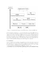
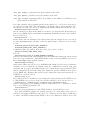
Although PETSc is written in C it works with objects. These objects are hierarchically organized which (ideally) makes it obsolete for the user to interact directly with
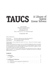
C-primitives or storage duration specifiers. Figure 2.1 illustrates the hierarchical organization of PETSc. An immediate consequence of the use of abstraction layers is that
1
Figure 2.1: Organizational diagram of the PETSc libraries. Taken from [BBB+ 10].
data is propagated ”bottom up”, i.e. top-level abstraction objects (like PDE-solvers) do
not access data in the underlying C-array directly but use methods on PETSc-vector and
-matrix objects. Hence if all low-level PETSc-objects are ported to CUDA all high-level
abstraction objects run on the GPU without any code modification. Following this idea
the current development version of PETSc introduces new vector and matrix implementations whose methods run entirely on the GPU using CUDA. In the following the basic
steps for setting up PETSc and using its new GPU support are explained.
2.1 Installation
A note of caution at the beginning: the installation procedure laid out here was tested
and is intended for a specific version of PETSc operated on specific hardware. This is by
no means meant to be a tutorial on how to set up PETSc in general. For readers looking
for such a tutorial the PETSc-homepage [BBB+ 11] is the place to go.
As mentioned above the GPU support of PETSc is realized by implementing new vector and matrix objects in CUDA. This implementation is done by using the CUDA
2
libraries Thrust [HB10] and Cusp [BG10]. Since at the time this text was written
Thrust, Cusp and PETSc were still under development it was necessary to obtain the
newest Cusp/Thrust versions from NVIDIA mercurial repositories in order to build the
newest PETSc development version. However, since this work was carried out in the
course of a PhD-seminar on GPU-computing the intention was to install PETSc on a
server reserved for seminar participants who were simultaneously pursuing other CUDAprogramming projects, many of them relying on Cusp/Thrust. Therefore constantly updating Cusp/Thrust seemed to be impractical and potentially jeopardous for the stability
of other projects. Hence the latest PETSc version compatible to the already installed
Cusp/Thrust libraries was chosen, namely version 15257:a0abdf539b1e from November
3rd, 2010.
The following installation procedure refers to the ”fermi”-server (IP: 143.50.47.245)
equipped with two GeForce GTX 480 on an ASUS P6T Deluxe V2 mainboard powered
by an Intel Core i7-920 CPU and 6GB Corsair XMS3 DIMM RAM running Ubuntu Linux
10.04.2 LTS 64bit. In the following we denote by the environmental variable PETSC_DIR
the full path to the PETSc home directory (for a local PETSc-installation on a *nix system
this is probably something like $HOME/petsc_dev/) while PETSC_ARCH specifies the local
architecture and compiler options (by using different PETS_ARCH one can handle different
sets of libraries). The versions of CUDA, Cusp and Thrust needed by PETSc are listed in
PETSC_DIR/config/PETSc/packages/cuda.py. Assuming that all NVIDIA software is
properly installed and nvcc is in the path one has ensure that LD_LIBRARY_PATH points to
the CUDA libraries (in our case using the bash: LD_LIBRARY_PATH=$LD_LIBRARY_PATH:/usr/local/cuda/li
then
export
LD_LIBRARY_PATH). Then PETSc is configured by issuing the following command in the
PETSC_DIR-directory:
./config/configure.py --with-debugging=1 --with-cuda=1 --with-cusp=1
--with-thrust=1 --with-mpi-dir=/usr/lib/openmpi --with-c2html=0
The meaning of the configure-options is given below:
with-debugging=1 compiles PETSc with debugging support (default). For performance
runs this should be turned off but for developing code it is highly recommended to
let it turned on (compare [BBB+ 10]).
with-cuda=1 compiles PETSc with CUDA support. This option is currently only available in development versions of PETSc. It checks whether compatible NVIDIA
kernel developer drivers are installed and all necessary binaries are in the path.
with-thrust=1 looks for Thrust in default locations (usually /usr/local/cuda/). If
Thrust is not installed in its default place the option --with-thrust-dir=
/path/to/thrust may be used. This option is currently only available in development versions of PETSc.
with-cusp=1 looks for Cusp in default locations (usually /usr/local/cuda/). If Cusp
is not installed in its default place the option --with-cusp-dir=/path/to/cusp
3
may be used. This option is currently only available in development versions of
PETSc.
with-mpi-dir=/usr/lib/openmpi points to the system’s MPI installation. The user
manual [BBB+ 10] claims that PETSc looks for MPI in all known standard locations.
Even so it did not find the openMPI installation on fermi though the location cannot
be called ”exotic”. However, this can as well be a problem of the developmentversion that may be fixed in future stable releases.
with-c2html=0 prevents PETSc from using the optional package c2html for its documentation ( used since c2html was not installed on fermi).
Note that if the GPU of the computer PETSc should be built on supports only single precision arithmetic (not the case with fermi’s two GeForce GTX 480) the option
--with-precision=single has to be given as well. It is further assumed that the system has a valid BLAS/LAPACK installation in default locations (otherwise the option --with-blas-lapack-dir=/path/to/libs has to be used). If BLAS/LAPACK is
not yet installed the option --download-f-blas-lapack=1 may be used to download
and build a local BLAS/LAPACK installation (the same can be done with MPI using
--download-mpich=1). However, due to performance reasons a system-wide installation
of MPI/BLAS/LAPACK should be preferred.
After successful completion of the configure-stage PETSc is built by
make all
The source code of PETSc has more than 80 MB, so building may take a while. When
the building is done the standard, i.e. non-CUDA, libraries can be tested by
make test
At present the only way to test the CUDA-functionality of PETSc is to build and run a
tutorial example for the nonlinear solvers:
cd PETSC_DIR/src/snes/examples/tutorials
make ex19
./ex19 -da_vec_type mpicuda -da_mat_type mpiaijcuda -pc_type none
-dmmg_nlevels 1 -da_grid_x 100 -da_grid_y 100 -log_summary -mat_no_inode
-preload off -cuda_synchronize
If both tests complete successfully PETSc can use NVIDIA GPUs.
2.2 Writing PETSc Code
Again a note of caution at the beginning: this section is not a programming guide. The
purpose of the following is to give the reader a first glimpse of how PETSc-programs are
written. Please refer to the user manual [BBB+ 10] for a comprehensive guide to PETSc
programming and consult the website [BBB+ 11] for numerous tutorial examples. Since
the author has written his code in C what follows refers to using PETSc from C. Note that
though all PETSc routines are accessible in the same way no matter if the user’s code is
written in C/C++, FORTRAN 77/90 or Python there are language specific differences
(e.g. FORTRAN starts indexing with 1, C/C++ and Python use zero-based indexing)
4
that have to be taken into account. Further details can be found on the PETSc-homepage
[BBB+ 11].
Shown here is the exemplary use of PETSc to solve the linear equation system Ax = b,
where A ∈ RN ×N is some regular matrix and x and b are vectors in RN . In order to use
PETSc from C the correct header has to be used, in our case
#include "petscksp.h"
which automatically includes all necessary low-level objects (PETSc-matrices, -vectors,
...). As laid out above PETSc’s abstraction-layer design (and consequently its CUDAfeatures) can only be exploited adequately if the user’s code is designed to solely use
PETSc-specific data structures. Hence we do not use standard C variables but initialize
the following PETSc-objects:
Mat A;
(the coefficient matrix A as PETSc-matrix)
Vec x, b;
(the solution x and the right hand side b as PETSc-vectors)
KSP ksp;
(a linear solver object)
PetscInt N;
(the dimension of the linear system as PETSc-integer)
Usually before anything else there should be the call
PetscInitialize(&argc,&args,(char *)0,help);
which initializes the PETSc database and calls MPI_Init(). Note that PetscInitialize()
has to be called before any PETSc-related function is used. Next the coefficient matrix
is created:
MatCreate(PETSC_COMM_WORLD,&A);
Every PETSc-object supports a basic interface (Create(), Get/SetName(),
Get/SetType(), Destroy(),...) similar to class methods in C++ (hence the Create()
routine can be seen as an equivalent to a C++ constructor). Therefore everything in this
section is only discussed for PETSc-matrices but works analogously for PETSc-vectors
(where it makes sense) only with the prefix Vec instead of Mat in the corresponding calls.
Note that PETSC_COMM_WORLD is the PETSc-version of MPI_COMM_WORLD (for details see
[BBB+ 10]). The size of the matrix has to be determined by
MatSetSizes(A,PETSC_DECIDE,PETSC_DECIDE,N,N);
By using PETSC_DECIDE the portions of the matrix held by each processor are determined
by PETSc (assuming that A is a parallel PETSc-matrix). The next call is one of the most
powerful features of PETSc: by using the method SetFromOptions() the implementation
type of a PETSc-object can be set at runtime using command line options (if no options
are given default values are used). Hence by calling
MatSetFromOptions(A);
the type of the PETSc-matrix A is either assumed to be parallel sparse on the CPU
(default) or it can be set by using the following command line options:
-mat_type aij sequential/parallel (depending on the number of MPI-processes) sparse
matrix on the CPU
-mat_type seqdense sequential dense matrix on the CPU
-mat_type mpidense parallel dense matrix on the CPU
5
-mat_type seqbaij sequential block sparse matrix on the CPU
-mat_type mpibaij parallel block sparse matrix on the CPU
-mat_type aijcuda sequential/parallel (depending on the number of MPI-processes)
sparse matrix on the GPU
Note that currently only sequential/parallel sparse matrices, i.e. no block or dense types,
are supported on the GPU. For performance reasons any (large) matrix should be preallocated before values are inserted. Assuming the PETSc-matrix A is parallel the call
MatMPIAIJSetPreallocation(A,...);
allocates memory for A given the number of nonzeros per diagonal and off-diagonal portion of A (see [BBB+ 10] for actual function arguments and further details). Once memory
has been allocated
MatSetValues(A,...);
inserts entries into the matrix A. Note that in this stage the matrix is not yet ready to
use since MatSetValues() generally caches the matrix entries. Therefore it is necessary
to call
MatAssemblyBegin(A,MAT_FINAL_ASSEMBLY);
MatAssemblyEnd(A,MAT_FINAL_ASSEMBLY);
to finally assemble the matrix. Next the solver object can be created:
KSPCreate(PETSC_COMM_WORLD,&ksp);
The call
KSPSetOperators(ksp,A,A,SAME_NONZERO_PATTERN);
tells the solver that A is the system matrix (here the matrix that defines the linear system
also serves as preconditioner). Like PETSc-matrices and -vectors any PETSc-solver object
has a SetFromOptions() method, namely
KSPSetFromOptions(ksp);
which either defines the solver to be a GMRES method with block Jacobi preconditioner
(default) or sets its attributes at runtime using the command line options -ksp_type
<solver> and -pc_type <preconditioner> (for a comprehensive list of available solvers
and preconditioners as well as the many other adjustable options of PETSc-solvers, please
refer to [BBB+ 10]). Having defined all necessary components of the linear system Ax = b
in PETSc we can now solve it:
KSPSolve(ksp,b,x);
The solution x can be examined or saved using the View() method of the PETSc-vector
x. When PETSc-objects are no longer needed they should be freed. In our case by
VecDestroy(x); VecDestroy(b); MatDestroy(A); KSPDestroy(ksp);
which is (analogously to the Create() method) equivalent to a C++ destructor. At the
end of every PETSc-program the call
PetscFinalize();
ensures the proper termination of the PETSc database and all MPI processes.
Note that all PETSc routines are passing references (to avoid unnecessary copies of
variables) and return a PETSc-specific error code. Therefore it is strongly recommended
to always call PETSc routines using PETSc’s error code (which was omitted above only
6
for the sake of brevity). The error code is also a PETSc variable that has to be declared
properly:
PetscErrorCode ierr;
Then a typical function call is for instance
ierr = MatCreate(PETSC_COMM_WORLD,&A);CHKERRQ(ierr);
where CHKERRQ(ierr) checks the error code, calls the appropriate handler and returns
(propagates errors from bottom up). This makes debugging of PETSc codes much easier.
Note further that it is of course possible to hard-code the implementation type of an
object, i.e. the use of the SetFromOptions()-method is not stringently required. If for
instance a matrix has to be a parallel MPI matrix for a program to work properly one
should prefer to explicitly write
ierr = MatSetType(A,MATMPIAIJ);CHKERRQ(ierr);
in the code over using MatSetFromOptions() in combination with the command line
argument -mat_type mpiaij. However, when running PETSc programs on NVIDIA
GPUs the SetFromOptions()-method should be employed in any case since debugging
on the GPU is currently very difficult (compare [BBB+ 11]).
2.3 Building and Running PETSc Programs
The author wants to emphasize again that this section (just as the previous one) refers
to using PETSc from C on a *nix-like system. If the reader wants to build PETSc code
written in C++, FORTRAN 77/90 or Python please consult the manual [BBB+ 10].
Since an average PETSc code is linked to (literally) dozens of libraries the use of Makefiles to automate the building process becomes mandatory. In the simplest case of one
source code file, namely first_code.c, a sample PETSc-Makefile is given below
PETSC_DIR = /home/user/petsc-3.1-p3
include ${PETSC_DIR}/conf/variables
include ${PETSC_DIR}/conf/rules
first_code: first_code.o chkopts ${CLINKER} -o first_code
first_code.o ${PETSC_LIB} ${RM} first_code.o
Further information about Makefiles for PETSc codes can be found in the corresponding
chapter of the manual [BBB+ 10]. The executable binary file first_code generated by the
command make first_code (assuming the building process succeeded without errors)
can be executed by
mpirun -np <n> ./first_code -petsc_option1 pvalue1 -petsc_option2 pvalue2
... -user_option1 uvalue1 -user_option2 uvalue2 ...
where <n> denotes the number of MPI processes. Note that any PETSc program can
use its own options (denoted as -user_option above) together with PETSc’s options.
A list of all available PETSc-options can be either found in the manual [BBB+ 10] or
by using ./first_code -help (which can of course be combined with the classical C
7
statement static char help = ”help text”; in the source code first_code.c). Examples of C code illustrating the use of PETSc and user-defined options can be found
online [BBB+ 11].
3 Numerical Results
This section presents the profiling results documenting the performance of PETSc version
15257:a0abdf539b1e on the fermi server. Note that since this work in progress version
of PETSc was already outdated by the time this text was written the results shown here
have to be seen as preliminary and do not reflect the final library performance.
3.1 Motivation: An Image Processing Problem
The following brief excursion to image processing is merely intended to provide a motivational problem that leads to a PDE which can be solved with PETSc. We consider an
image denoising problem (the following derivation is mainly taken from [AK06, Chap. 3]).
Let Ω := [1, N ]2 ⊂ R2 with N ∈ N and f, u : Ω → R. Assume that u is the unknown
original image and f is the given degraded data (for the sake of simplicity we consider
here only gray-scale images; otherwise u and f would not be scalar but vector valued).
We want to recover u from f which is a so-called image reconstruction problem. Thus
we first of all need a model linking u to f . One of the simplest and most widely used
(compare [AK06, Chap. 3]) is the linear relation
f = u + η,
where η is a noise term. To solve this inverse problem we make some assumptions on η:
suppose η is white Gaussian noise then according to the maximum likelihood principle
the solution of the least squares problem
ˆ
(3.1)
inf
|f − u|2 dx,
u
Ω
is an approximation to the original image. However, in this form u ≡ f is the minimizer
of (3.1). Thus we introduce a regularization term. We define the functional
ˆ
ˆ
1
1
2
(3.2)
J(u) :=
|f − u| dx +
|∇u|2 dx,
2 Ω
2 Ω
and consider the minimization problem
(3.3)
min J(u).
u∈H 1 (Ω)
Note that for u ∈ H 1 (Ω) and f ∈ L2 (Ω) problem (3.3) is well defined and admits a unique
solution (see for instance [AK06, Chap. 3]). Thus the use of min instead of inf in (3.3) is
justified. Note further that usually the second term enters the cost functional J with an
additional (multiplicative) parameter λ. However, in practice choosing λ ”correctly” is
8
not trivial. Hence for the sake of simplicity (but at the expense of the solution’s quality)
we relinquish the use of λ.
The first term in (3.2) measures the fidelity of u to the given data f while the second
term (first introduced by Tikhonov and Arsenin [TA77] in 1977) penalizes oscillations in
the gradient of u. This means that the minimizer of (3.2) is not only supposed to be
close to the given data but also a solution with low gradient and hence low noise level is
favored.
The classical approach to solve the minimization problem (3.3) is to use variational
calculus: we compute the Gâteaux derivative of J in an arbitrary direction v ∈ C ∞ (Ω̄),
i.e. we compute
δJ
d
(u; v) :=
J(u + sv)
,
δu
ds
s=0
for some scalar parameter s ∈ R. This yields
ˆ
ˆ
1
d
d 1
2
2
|f − (u + sv)| dx +
|∇u + s∇v| dx J(u + sv)
=
ds
ds 2 Ω
2 Ω
s=0
s=0
ˆ
ˆ
= (f − u)v dx +
∇u · ∇v dx
Ω
Ω
ˆ
ˆ
ˆ
= (f − u)v dx +
v∇u · ndS −
v∆u dx,
Ω
∂Ω
Ω
where we used partial integration to shift derivatives from v to u. The weak necessary
optimality condition for the minimization of J is
δJ
(u; v) = 0,
∀v ∈ C ∞ (Ω̄).
δu
Assuming that u is sufficiently regular we may apply the fundamental Lemma of calculus
of variations to obtain

 ∆u + u =f in Ω,
∂u

=0 on ∂Ω,
∂n
the so-called Euler–Lagrange equations associated to the optimization problem (3.3).
However, for the sake of notation in the numerical community we rewrite it into

 −∆u − u = −f in Ω,
(3.4)
∂u

= 0 on ∂Ω.
∂n
To solve the PDE (3.4) with PETSc we discretize it using central finite differences with a
unit step size h = 1. Then the discrete version of the Laplacian operator with Neumann
boundary conditions under lexicographic ordering is a large sparse block matrix:


B −I

 −I C −I


2
2


..
..
..
−∆h := 
 ∈ RN ×N ,
.
.
.



−I C −I 
−I B
9
with blocks

3 −1
 −1 4 −1


..
..
C := 
.
.


−1




 ∈ RN ×N ,
.

4 −1 
−1 3
..
and
B := C − IN ,
where IN ∈ RN ×N is the identity matrix and N denotes the image dimension. Let
2
2
f~ ∈ RN and ~u ∈ RN denote the discrete versions of the noisy image and the original
image under lexicographic ordering respectively. Then the Euler–Lagrange equations
(3.4) are discretized by
(3.5)
A~u = f~,
where
A := −∆h − IN 2 .
Note that it is well known that the Laplace operator has very strong smoothing properties
and thus tends to blur edges [AK06]. Since the Laplacian in the Euler–Lagrange equation
(3.4) arises from the L2 -norm of the gradient of u in the corresponding weak formulation
(3.2) the idea is to use the L1 -norm in (3.2) instead. One of the first who followed this
idea were Rudin, Osher and Fatemi in their ground breaking work [ROF92]. Using the
L1 -norm of ∇u, also called total variation of u, proved to be highly successful in practice.
And when Chambolle published a projection algorithm [Cha04] the numerical solution
of total variation based models could be realized in a computationally very efficient way.
However, having in mind that the purpose of this work was to test PETSc’s performance
on NVIDIA GPUs the use of total variation minimization together with Chambolle’s
algorithm did not seem suitable since it does not involve the solution of linear systems.
Thus we employed the above model leading to the PDE (3.4) although the approach is
not state of the art (a novel approach that generalizes the total variation and overcomes
some of its drawbacks is the so-called total generalized variation [BKP09]).
3.2 Performance Tests
We solve the discrete Euler–Lagrange equation (3.5) using PETSc and compare its performance on the CPU and on the GPU. All runs were carried out with PETSc version
15257:a0abdf539b1e on the fermi server described above. This PETSc version supports
the following GPU features:
• two CUDA vector implementations: seqcuda and mpicuda
• two CUDA matrix implementations: seqaijcuda and mpiaijcuda
10
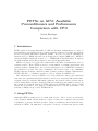
(a)
(b)
(c)
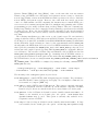
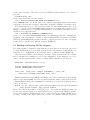
Figure 3.1: The original gray scale test image (a), the noisy image f (b) and the computed
reconstruction u (c).
• all Krylov methods except ibcgs (an improved stabilized version of the bi-conjugate
gradient squared method, see [YB02]) run on the GPU (ibcgs violates PETSc’s
hierarchical abstraction layer design by directly accessing data in the underlying C
arrays; hence it needs to be rewritten to run on the GPU)
• the preconditioners jacobi, bjacobi (block Jacobi) and asm (an restricted additive
Schwarz method, see [DW]) run on the GPU
Note that the discrete Laplacian ∆h is a textbook example of a sparse block matrix
that can be stored memory efficiently by exploiting its inherent symmetries and block
structure. However, since the PETSc version used here only supports sequential or parallel sparse matrices on the GPU neither the block structure nor symmetries of ∆h have
been taken into account in the implementation of (3.5). Nevertheless, as indicated above
PETSc provides matrix formats on the CPU which can utilize symmetry and block structure of a matrix. Even so, for better comparison to the GPU performance these formats
have not been used.
The code for solving (3.5) was developed using the SetFromOptions() method. This
way it was possible to run the same code both on the CPU and on the GPU using only
different command line options. After finalization of the implementation process PETSc
was recompiled using the --with-debugging=0 option to obtain better performance in
the test runs.
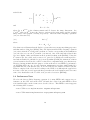
The original gray scale test image used here is depicted in Figure 3.1 (a). The noisy
image f (depicted in Figure 3.1 (b)) was obtained by adding 35% Gaussian white noise
to the original image. The image dimension was N = 1290 thus giving N 2 = 1 664 100
unknowns and 8 315 340 nonzero entries in the coefficient matrix A of (3.5).
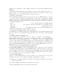
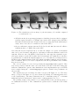
The profiling results of the solution of (3.5) using PETSc for the given noisy image f
are summarized in Table 1. The command line options used to obtain the CPU results
were
11
CPU/GPU
Preconditioner
Iterations
PETSc-CPU
bjacobi
jacobi
asm
bjacobi
jacobi
asm
6
15
5
6
15
5
PETSc-GPU
Time (sec)
(All/Solve/Copy)
2.3/0.2/–
2.7/0.5/–
2.2/0.2/–
1.9/0.1/0.05
1.7/0.1/0.01
2.1/0.1/0.1
Memory (MB)
348
223
271
304
268
242
Table 1: Profiling results of solving (3.5) using PETSc on the fermi server with two MPI
processes. The first three rows show the CPU-performance of PETSc, the last
three rows illustrate its GPU-performance. The default linear solver GMRES
with standard options has been used. The second column indicates the employed preconditioners, the third column shows how many GMRES-iterations
were needed to satisfy the default convergence criterion. The fourth column
depicts the runtime (in seconds) of the whole program, the time needed to solve
(3.5) and the time spent copying data from host to device and vice versa. Finally
the rightmost column shows PETSc’s memory consumption (in Megabytes).
-mat_type mpiaij -vec_type mpi -pc_type jacobi/bjacobi/asm
-log_summary -memory_info
for the GPU results the options
-mat_type mpiaijcuda -vec_type mpicuda -pc_type jacobi/bjacobi/asm
-log_summary -memory_info
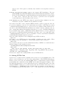
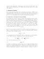
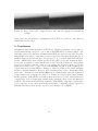
have been used. The computed solution u is depicted in Figure 3.1 (c). For better
visual evaluation the upper right portion of the corrupted image f and the computed
reconstruction u is given in Figure 3.2. Note that the computed image u still contains
noise and suffers from blurred edges. These are known negative effects of employing the
Laplacian for image denoising that can be reduced by either including a regularization
parameter λ (as explained in the previous section) or by utilizing a more sophisticated
cost functional, e.g. a total variation based cost. However, as stated above the purpose of
this work was not to obtain a preferably well reconstructed image but to profile PETSc’s
performance on the GPU.
The performance boost by running our code on the GPU using this version of PETSc
was surprisingly small. It seems that the (preliminary) implementation of the preconditioners on the GPU is not memory efficient yet: when using the restricted additive
Schwarz preconditioner asm copying data back and forth between host and device took
approximately as long as solving the system (3.5). For the block Jacobi preconditioner
bjacobi the copy-time summed up to 50% of the solution time. The most efficient preconditioner (referring to the copying time) was the Jacobi preconditioner in our profiling
runs. However, note that these results have to be interpreted with caution: the PETSc
mailing list confirms that newer versions of Cusp/Thrust/PETSc do not exhibit the same
problems. But for reasons explained above these new versions could not be tested on
12
Figure 3.2: Image detail of the corrupted data f (left) and the computed reconstruction
u (right).
fermi. Moreover, the memory consumption given in Table 1 seems to be inaccurate in
this PETSc version either.
4 Conclusions
Summarized the CUDA capabilities of PETSc are extremely promising. People who are
already using PETSc can ”port” code to run on NVIDIA GPUs by using a simple command line option. For anyone not familiar with PETSc the way of doing GPU programming PETSc offers may be compelling for two reasons: first (and most important) due to
PETSc’s abstraction layers the user does not have to be concerned with GPU hardware
details - PETSc hides away CUDA specifics in the GPU-vector and -matrix methods.
Second the possibility to easily switch between CPU and GPU makes the development
process very flexible: if in the course of code-writing the decision is made to test the
application on the GPU it can be done with minimal amount of work (assuming the
code is written solely using PETSc’s datatypes). Hence in terms of CPU/GPU flexibility
PETSc is currently unrivaled. However, these advantages have a price: mastering PETSc
takes time. Though the user manual [BBB+ 10] is comprehensive and well structured
it takes rather long (compared to classic C or Python at least) to write a first working
PETSc-program. Thus PETSc is probably most attractive to people dealing with very
complex large scale problems that demand high performance state of the art numerical
methods. The newly included CUDA capabilities make PETSc competitive (and in some
respect superior) to any other modern high performance computing software but are at
this time probably not the decisive factor to port existing code to PETSc.
13
References
[AK06]
G. Aubert and P. Kornprobst. Mathematical Problems In Image Processing,
volume 147 of Applied Mathematical Sciences. Springer, 2nd edition, 2006.
[BBB+ 10] S. Balay, J. Brown, K. Buschelman, V. Eijkhout, W.D. Gropp, D. Kaushik,
M.G. Knepley, L.C. McInnes, B.F. Smith, and H. Zhang. PETSc users manual. Technical Report ANL-95/11 - Revision 3.1, Argonne National Laboratory, 2010.
[BBB+ 11] S. Balay, J. Brown, K. Buschelman, W.D. Gropp, D. Kaushik, M.G. Knepley, L.C. McInnes, B.F. Smith, and H. Zhang. PETSc Web page, 2011.
http://www.mcs.anl.gov/petsc.
[BG10]
N. Bell and M. Garland. Cusp: Generic parallel algorithms for sparse matrix
and graph computations, 2010. Version 0.1.0.
[BKP09]
K. Bredies, K. Kunisch, and T. Pock. Total generalized variation. Technical
report, Institute for Mathematics and Scientific Computing, Karl–Franzens
University Graz, Austria, 2009.
[Cha04]
A. Chambolle. An algorithm for total variation minimization and applications.
Journal of Mathematical Imaging and Vision, 20(1–2):89–97, March 2004.
[DW]
M. Dryja and O.B. Widlund. An additive variant of the schwarz alternating
method for the case of many subregions. Technical report, Courant Institute,
New York University.
[HB10]
J. Hoberock and N. Bell. Thrust: A parallel template library, 2010. Version
1.3.0.
[ROF92]
L. Rudin, S. Osher, and E. Fatemi. Nonlinear total variation based noise
removal algorithms. Journal of Physics D: Applied Physics, 60:259–268, 1992.
[TA77]
A.N. Tikhonov and V.Y. Arsenin. Solutions of Ill-Posed Problems. Winston
and Sons, Washington D.C., 1977.
[YB02]
L.T. Yand and R. Brent. The improved bicgstab method for large and sparse
unsymmetric linear systems on parallel distributed memory architectures. In
Proceedings of the Fifth International Conference on Algorithms and Architectures for Parallel Processing. IEEE, 2002.
14