Download PETSc - University of Saskatchewan

PETSc – Portable, Extensible
Toolkit for Scientific Computing
Raymond J. Spiteri
Lecture Notes for CMPT 898:
Numerical Software
University of Saskatchewan
Objectives
• Introduction to PETSc
• Installation and use
• Linear system solvers
• Nonlinear system solvers
• ODE/DAE solvers
1
Introduction to PETSc
PETSc (|"petsi:|) stands for the Portable, Extensible
Toolkit for Scientific Computing.
• suite of libraries (data structures, objects/methods,
functions/subroutines) produced and maintained by
Argonne National Laboratory for the solution of
scientific applications modelled by partial differential
equations (PDEs)
• intended for use in large-scale (HPC) applications
• includes a large suite of parallel linear and nonlinear
algebraic equation solvers as well as ODE solvers
• sets up many of the mechanisms required for parallel
application codes, including parallel matrix and
vector assembly
• integrates BLAS (Basic Linear Algebra Subprograms)
and LAPACK (Linear Algebra PACKage) as the
back-end for basic vector and matrix operations
2
Introduction to PETSc
• can be used in Windows, Mac, and Linux
• written in C
• can be used within C, C++, Fortran, Python, and
Matlab applications
• interfaces with many other software packages,
making it easy to try new methods and solvers
• used in many applications, including heart
simulation, carbon sequestration, ground water flow,
medical imaging, and quantum computing
See http://www.mcs.anl.gov/petsc/ for details.
3
Software accessible through PETSc
PETSc can interface with other software applications,
including
• ADIC/ADIFOR for computing sparse Jacobian
matrices by automatic differentiation
• The Unsymmetric MultiFrontal Sparse LU
factorization PACKage (UMFPACK) for the direct
solution of unsymmetric sparse linear systems
• The MUltifrontal Massively Parallel sparse direct
Solver (MUMPS) for large sparse linear systems
• SuperLU, a library for the direct solution of large,
sparse nonsymmetric linear systems
• Prometheus, a scalable, unstructured finite element
solver
• Trilinos/ML, a multigrid preconditioner package
4
Software currently using PETSc
PETSc is used by many software packages, including
• TAO: Toolkit for Advanced Optimization
• SLEPc: Scalable Library for Eigenvalue Problems
• deal.II: an adaptive finite element solver
• Chaste:
Cancer,
Environment
Heart,
and
Soft
Tissue
5
Features of PETSc
Features of PETSc include:
• intended to be easy to learn and use for beginners
(extensive examples and tutorials)
• control over numerical methods for advanced users
• parallel vectors and matrices
• parallel linear system solvers based on Krylov
subspace methods, including Conjugate Gradient
• parallel preconditioners
• parallel nonlinear solvers based on Newton’s method
• parallel ODE solvers
• extensive documentation; complete user’s manual
http://www.mcs.anl.gov/petsc/petsc-current/docs/manual.pdf
6
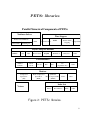
PETSc Library Hierarchy
Level of
Abstraction
Application Codes
TS
(Time Stepping)
SNES
(Nonlinear Equations Solvers)
PC
(Preconditioners)
Matrices
KSP
(Krylov Subspace Methods)
Vectors
BLAS
Index Sets
MPI
Figure 1: Hierarchy of PETSc libraries.
7
PETSc libraries
Parallel Numerical Components of PETSc
Nonlinear Solvers
Time Steppers
Newton−based Methods
Other
Line Search
IMEX
General Linear
Pseudo−Time
Runge−Kutta
Stepping
Trust Region
Krylov Subspace Methods
GMRES
CG
CGS
Bi−CG−Stab
TFQMR
Richardson
Chebychev
Other
Preconditioners
Additive
Schwarz
Block
Jacobi
Jacobi
ILU
ICC
LU
(sequential only)
Other
Matrices
Compressed
Sparse Row
(AIJ)
Block Compressed
Symmetric
Sparse Row
Block Compressed Row Dense
(BAIJ)
(SBAIJ)
Other
Index Sets
Vectors
Indices
Block Indices
Stride
Other
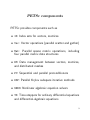
Figure 2: PETSc libraries.
8
PETSc components
PETSc provides components such as
• IS: Index sets for vectors, matrices
• Vec: Vector operations (parallel scatter and gather)
• Mat: Parallel sparse matrix operations, including
four parallel matrix data structures
• DM: Data management between vectors, matrices,
and distributed meshes
• PC: Sequential and parallel preconditioners
• KSP: Parallel Krylov subspace iterative methods
• SNES: Nonlinear algebraic equation solvers
• TS: Time-steppers for ordinary differential equations
and differential-algebraic equations
9
Parallelism in PETSc
PETSc uses the Message Passing Interface (MPI) for
its parallelization.
The calls made to MPI in PETSc are at a high level
and mostly hidden from the user; typically users should
not have to call MPI directly themselves although they
are free to do so.
Nonetheless, familiarity with the basic concepts of
message passing and distributed memory computing is
essential when using PETSc.
In these notes, we assume users have this basic level
of familiarity.
10
Installation
PETSc has comprehensive instructions for installation
on Linux and Windows with a variety of configurations.
PETSc can download and install its own dependencies,
making the installation process easy for new users.
One way to install PETSc is to download it from the
main website:
http://www.mcs.anl.gov/petsc/download/index.html
Assuming PETSc is at version xxxx, we unpack the
downloaded tar file via the following command:
tar xzvf petsc-xxxx.tar.gz
Another way is to download it using mercurial via
hg clone https://bitbucket.org/petsc/petsc-3.3 petsc-3.3
hg clone https://bitbucket.org/petsc/buildsystem-3.3 petsc-3.3/config/BuildSystem
11
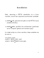
Installation
Next, assuming a PETSc installation on a Linux
machine, we set two important environment variables:
• PETSC DIR: gives the full path to the PETSc home
(install) directory
• PETSC ARCH: specifies the architecture (particular
set of compiler options and machine type)
In a bash script on a linux machine, these variables can
be set via
cd petsc-xxxx
export PETSC DIR=`pwd`
export PETSC ARCH=linux-gnu
12
Installation
The next step is to configure PETSc so that it knows
where libraries are installed and what additional libraries
are required the installation.
For example,
./config/configure.py --download-f-blas-lapack=1
--download-openmpi=yes --with-cc=gcc --with-fc=gfortran
This example downloads and installs the MPI library
openmpi independent of any existing installation.
This is the recommended approach (assuming sufficient
disk space, etc.).
However, PETSc can be made to work with existing
MPI installations.
13
Installation
Now, PETSc must be built and tested.
This is done by executing the following command:
make all test
It is also easy to try running one of the many PETSc
examples provided (making sure the environment
variables PETSC DIR and PETSC ARCH are set):
cd $PETSC DIR/src/ksp/ksp/examples/tutorials
make ex1
mpiexec -np 1 ./ex1
If you run into trouble using mpiexec, it may be that
the path to mpiexec has not been set.
From the bash shell, the following command may help
export PATH=$PATH:$PETSC DIR/$PETSC ARCH/bin
Note that this example is for a single process (the value
passed to the number of processes flag, np, is 1).
14
Installation
For the corresponding parallel example, we can try
make ex23
mpiexec -np 2 ./ex23
We can pass any value to np up to the number of
processes allowed on the computer being used.
In this directory of tutorials and examples, each
example has C or Fortran code and an HTML file
that describes the code in detail.
For complete installation instructions, including
instructions for installation under Windows, see the
installation page available from PETSc:
http://www.mcs.anl.gov/petsc/documentation/installation.html
15
Running PETSc
All PETSc programs support the -h or -help option
as well as the -v or -version option.
The following is a list of some of the other more useful
options (a complete list is available via the -h option).
• -log summary: summarize program performance
• -fp trap: stop on floating-point exception
• -malloc dump: list free memory at end of run
• -malloc debug: enable memory tracing
• -info: print detailed output as program runs
• -options file <filename> read options from file
It is also possible start all processes in a debugger or
start the debugger only when encountering an error.
16
Writing PETSc Programs
It is easy to run the examples that come with PETSc;
but to create and run applications of your own,
additional work is required.
A practical starting strategy is to find an example in
the many examples provided that most closely matches
the problem you wish to solve.
After ensuring this example can be built and run
successfully, copy the contents into a new directory,
then use the programs and makefile as a starting point
from which to being solving your problem.
An important part of this process is the construction
of the makefile.
A makefile is a file containing a set of instructions
required to build an executable from source code.
An excellent introduction to makefiles as well as other
basic computing skills is available at
http://software-carpentry.org
17
Writing PETSc Programs
Consider again the first example ex1.
The makefile to build this example looks like
#Makefile to build ex1
include ${PETSC DIR}/conf/base
ex1: ex1.o chkopts
-${CLINKER} -o ex1 ex1.o
$RM ex1.o
${PETSC KSP LIB}
Because this example is written in C, the C linker
${CLINKER} is used.
This is an example of an internal environment variable
known to and used by PETSc.
Another environment variable, ${PETSC KSP LIB},
gives the linker the information required to build
against the PETSc libraries.
Finally, recall that the ${PETSC DIR} environment
variable was set when PETSc was installed and stores
the path to the main PETSc directory.
18
Writing PETSc Programs
The general form of a PETSc program includes the
following structure:
• Programs in C begin with
PetscInitialize(int *argc,char ***argv,char *file,char *help);
where argc, argv are the usual command-line
arguments, or in Fortran
call PetscInitialize(character(*) file,integer ierr)
PetscInitialize() calls MPI Init() if MPI has
not been previously initialized.
If MPI needs to be initialized directly (or is initialized
by some other library), MPI Init() can be called
before PetscInitialize().
By default,
PetscInitialize() sets the
PETSc world communicator PETSC COMM WORLD to
MPI COMM WORLD.
19
Writing PETSc Programs
• All PETSc routines return an integer indicating
whether an error has occurred during the call.
The error code is nonzero if an error has been
detected; otherwise, it is zero.
It is a good idea to check this error code after every
call to a PETSc routine!
• All PETSc programs should call PetscFinalize()
before finishing.
The C and Fortran syntax respectively are
PetscFinalize();
call PetscFinalize(ierr)
If MPI was initialized from PetscInitialize(),
PetscFinalize() calls MPI Finalize(); otherwise
MPI Finalize() must be called directly.
20
Solving Ax = b in serial
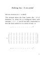
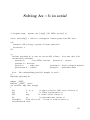
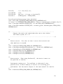
We now examine ex1.c in detail.
This example solves the linear system Ax = b of
dimension 10, where A is a tridiagonal matrix with
elements [−1 2 −1] and b has been constructed so
that the exact solution x is a vector of ones, i.e.,
x=








A=







2
−1
0
0
0
0
0
0
0
0
b=
1
−1
2
−1
0
0
0
0
0
0
0
1
1
1
0
−1
2
−1
0
0
0
0
0
0
0
1
0
0
−1
2
−1
0
0
0
0
0
0
0
1
0
0
0
−1
2
−1
0
0
0
0
0
1
1
0
0
0
0
−1
2
−1
0
0
0
0
1
0
0
0
0
0
−1
2
−1
0
0
0
0
1
1
0
0
0
0
0
0
−1
2
−1
0
0
T
,
0
0
0
0
0
0
0
−1
2
−1
1
T
0
0
0
0
0
0
0
0
−1
2








,







.
21
Solving Ax = b in serial
/* Program usage:
mpiexec ex1 [-help] [all PETSc options] */
static char help[] = "Solves a tridiagonal linear system with KSP.\n\n";
/*T
Concepts: KSP solving a system of linear equations
Processors: 1
T*/
/*
Include "petscksp.h" so that we can use KSP solvers. Note that this file
automatically includes:
petscsys.h
- base PETSc routines
petscvec.h - vectors
petscmat.h - matrices
petscis.h
- index sets
petscksp.h - Krylov subspace methods
petscviewer.h - viewers
petscpc.h - preconditioners
Note:
The corresponding parallel example is ex23.c
*/
#include <petscksp.h>
#undef __FUNCT__
#define __FUNCT__ "main"
int main(int argc,char **args)
{
Vec
x, b, u;
/* approx solution, RHS, exact solution */
Mat
A;
/* linear system matrix */
KSP
ksp;
/* linear solver context */
PC
pc;
/* preconditioner context */
PetscReal
norm,tol=1.e-14; /* norm of solution error */
PetscErrorCode ierr;
22
PetscInt
PetscMPIInt
PetscScalar
PetscBool
i,n = 10,col[3],its;
size;
neg_one = -1.0,one = 1.0,value[3];
nonzeroguess = PETSC_FALSE;
PetscInitialize(&argc,&args,(char *)0,help);
ierr = MPI_Comm_size(PETSC_COMM_WORLD,&size);CHKERRQ(ierr);
if (size != 1) SETERRQ(PETSC_COMM_WORLD,1,"This is a uniprocessor example only!");
ierr = PetscOptionsGetInt(PETSC_NULL,"-n",&n,PETSC_NULL);CHKERRQ(ierr);
ierr = PetscOptionsGetBool(PETSC_NULL,"-nonzero_guess",&nonzeroguess,PETSC_NULL);
CHKERRQ(ierr);
/* - - - - - - - - - - - - - - - - - - - - - - - - - - - - - - - - - Compute the matrix and right-hand-side vector that define
the linear system, Ax = b.
- - - - - - - - - - - - - - - - - - - - - - - - - - - - - - - - - - */
/*
Create vectors. Note that we form 1 vector from scratch and
then duplicate as needed.
*/
ierr
ierr
ierr
ierr
ierr
ierr
=
=
=
=
=
=
VecCreate(PETSC_COMM_WORLD,&x);CHKERRQ(ierr);
PetscObjectSetName((PetscObject) x, "Solution");CHKERRQ(ierr);
VecSetSizes(x,PETSC_DECIDE,n);CHKERRQ(ierr);
VecSetFromOptions(x);CHKERRQ(ierr);
VecDuplicate(x,&b);CHKERRQ(ierr);
VecDuplicate(x,&u);CHKERRQ(ierr);
/*
Create matrix. When using MatCreate(), the matrix format can
be specified at runtime.
Performance tuning note: For problems of substantial size,
preallocation of matrix memory is crucial for attaining good
performance. See the matrix chapter of the users manual for details.
*/
ierr = MatCreate(PETSC_COMM_WORLD,&A);CHKERRQ(ierr);
23
ierr = MatSetSizes(A,PETSC_DECIDE,PETSC_DECIDE,n,n);CHKERRQ(ierr);
ierr = MatSetFromOptions(A);CHKERRQ(ierr);
ierr = MatSetUp(A);CHKERRQ(ierr);
/*
Assemble matrix
*/
value[0] = -1.0; value[1] = 2.0; value[2] = -1.0;
for (i=1; i<n-1; i++) {
col[0] = i-1; col[1] = i; col[2] = i+1;
ierr = MatSetValues(A,1,&i,3,col,value,INSERT_VALUES);CHKERRQ(ierr);
}
i = n - 1; col[0] = n - 2; col[1] = n - 1;
ierr = MatSetValues(A,1,&i,2,col,value,INSERT_VALUES);CHKERRQ(ierr);
i = 0; col[0] = 0; col[1] = 1; value[0] = 2.0; value[1] = -1.0;
ierr = MatSetValues(A,1,&i,2,col,value,INSERT_VALUES);CHKERRQ(ierr);
ierr = MatAssemblyBegin(A,MAT_FINAL_ASSEMBLY);CHKERRQ(ierr);
ierr = MatAssemblyEnd(A,MAT_FINAL_ASSEMBLY);CHKERRQ(ierr);
/*
Set exact solution; then compute right-hand-side vector.
*/
ierr = VecSet(u,one);CHKERRQ(ierr);
ierr = MatMult(A,u,b);CHKERRQ(ierr);
/* - - - - - - - - - - - - - - - - - - - - - - - - - - - - - - - - - Create the linear solver and set various options
- - - - - - - - - - - - - - - - - - - - - - - - - - - - - - - - - - */
/*
Create linear solver context
*/
ierr = KSPCreate(PETSC_COMM_WORLD,&ksp);CHKERRQ(ierr);
/*
Set operators. Here the matrix that defines the linear system
also serves as the preconditioning matrix.
*/
ierr = KSPSetOperators(ksp,A,A,DIFFERENT_NONZERO_PATTERN);CHKERRQ(ierr);
24
/*
Set linear solver defaults for this problem (optional).
- By extracting the KSP and PC contexts from the KSP context,
we can then directly call any KSP and PC routines to set
various options.
- The following four statements are optional; all of these
parameters could alternatively be specified at runtime via
KSPSetFromOptions();
*/
ierr = KSPGetPC(ksp,&pc);CHKERRQ(ierr);
ierr = PCSetType(pc,PCJACOBI);CHKERRQ(ierr);
ierr = KSPSetTolerances(ksp,1.e-5,PETSC_DEFAULT,PETSC_DEFAULT,PETSC_DEFAULT);
CHKERRQ(ierr);
/*
Set runtime options, e.g.,
-ksp_type <type> -pc_type <type> -ksp_monitor -ksp_rtol <rtol>
These options will override those specified above as long as
KSPSetFromOptions() is called _after_ any other customization
routines.
*/
ierr = KSPSetFromOptions(ksp);CHKERRQ(ierr);
if (nonzeroguess) {
PetscScalar p = .5;
ierr = VecSet(x,p);CHKERRQ(ierr);
ierr = KSPSetInitialGuessNonzero(ksp,PETSC_TRUE);CHKERRQ(ierr);
}
/* - - - - - - - - - - - - - - - - - - - - - - - - - - - - - - - - - Solve the linear system
- - - - - - - - - - - - - - - - - - - - - - - - - - - - - - - - - - */
/*
Solve linear system
*/
ierr = KSPSolve(ksp,b,x);CHKERRQ(ierr);
25
/*
View solver info; we could instead use the option -ksp_view to
print this info to the screen at the conclusion of KSPSolve().
*/
ierr = KSPView(ksp,PETSC_VIEWER_STDOUT_WORLD);CHKERRQ(ierr);
/* - - - - - - - - - - - - - - - - - - - - - - - - - - - - - - - - - Check solution and clean up
- - - - - - - - - - - - - - - - - - - - - - - - - - - - - - - - - - */
/*
Check the error
*/
ierr = VecAXPY(x,neg_one,u);CHKERRQ(ierr);
ierr = VecNorm(x,NORM_2,&norm);CHKERRQ(ierr);
ierr = KSPGetIterationNumber(ksp,&its);CHKERRQ(ierr);
if (norm > tol){
ierr = PetscPrintf(PETSC_COMM_WORLD,"Norm of error %G, Iterations %D\n",
norm,its);CHKERRQ(ierr);
}
/*
Free work space. All PETSc objects should be destroyed when they
are no longer needed.
*/
ierr = VecDestroy(&x);CHKERRQ(ierr); ierr = VecDestroy(&u);CHKERRQ(ierr);
ierr = VecDestroy(&b);CHKERRQ(ierr); ierr = MatDestroy(&A);CHKERRQ(ierr);
ierr = KSPDestroy(&ksp);CHKERRQ(ierr);
/*
Always call PetscFinalize() before exiting a program. This routine
- finalizes the PETSc libraries as well as MPI
- provides summary and diagnostic information if certain runtime
options are chosen (e.g., -log_summary).
*/
ierr = PetscFinalize();
return 0;
}
26
Solving Ax = b in serial
Notes:
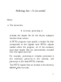
• The instruction
# include petscksp.h
includes the header file for the Krylov subspace
iterative linear solvers.
A PETSc program must specify a header file that
corresponds to the highest level PETSc objects
needed within the program; all of the necessary
lower-level header files are automatically included
from the higher-level call.
For example, petscksp.h includes petscmat.h
(for matrices), petscvec.h (for vectors), and
petscsys.h (for base PETSc routines).
The PETSc header files are located in the directory
$PETSC DIR/include.
27
Solving Ax = b in serial
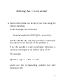
• Input control data can be set at run time using the
options database.
In this example, the command
PetscOptionsGetInt(PETSC NULL,-n,&n,&flg);
checks whether the user has provided a commandline option to set the size of the problem n.
If so, the variable n is set accordingly; otherwise, n
remains unchanged at its default value of 10.
For example,
mpiexec -np 1 ./ex1 -n 100
would run the corresponding problem but with
dimension 100.
28
Solving Ax = b in serial
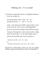
• Parallel or sequential vectors x of (global) dimension
M can be created via
VecCreate(MPI_Comm comm, Vec *x);
VecSetSizes(Vec x, int m, int M);
where comm denotes the MPI communicator and m
is the local size, which may be PETSC DECIDE.
As such, the vectors created as described are empty.
The type of storage for a vector may be set by calling
either VecSetType() or VecSetFromOptions().
Vectors of the same type can be formed via
VecDuplicate(Vec old, Vec *new);
or
VecDuplicateVecs(Vec old,int n,Vec **new);
Sequential or distributed vectors can also be created
directly using VecCreateSeq() and VecCreateMPI().
29
Solving Ax = b in serial
These constructs are useful because they allow one
to write library code that does not depend on the
particular format of the vectors being used.
Instead, PETSc automatically and correctly creates
work vectors based on the existing vector.
As usual, when a vector or array of vectors is no longer
needed, it should be destroyed via
VecDestroy(Vec *x);
or
VecDestroyVecs(PetscInt n,Vec **vecs);
Vectors that use an array provided by the user (rather
than having PETSc internally allocate the array space)
can be created via
VecCreateSeqWithArray(PETSC COMM SELF,int bs,int n,PetscScalar *array,Vec *V);
and
VecCreateMPIWithArray(MPI Comm comm,int bs,int n,int N,PetscScalar *array,Vec *vv);
where n must be given (i.e., not PETSC DECIDE) and
there must be enough space: n*sizeof(PetscScalar).
30
Solving Ax = b in serial
Vector components can be set (“inserted”) via
VecSetValues(Vec x, int n, int *indices, PetscScalar *values, INSERT_VALUES);
Vector components can be set to the same (scalar)
value via
VecSet(Vec x, PetscScalar value);
Note the use of the PETSc variable type PetscScalar.
The PetscScalar type is defined to be double
in C/C++ (or double precision in Fortran) for
versions of PETSc that have not been compiled for use
with complex numbers.
The PetscScalar data type enables code to be reused when the PETSc libraries have been compiled for
use with complex numbers.
Values can be added to existing components of a vector
by using the ADD VALUES insert mode.
31
Solving Ax = b in serial
Assigning individual values to components of a vector
is more complicated two-step process, but with the
advantage that the end result is more efficient
underlying parallel code.
The first call is to
VecSetValues(Vec x,int n,int *indices,PetscScalar *values,INSERT VALUES);
where n gives the number of components to be set in
this call.
The integer array indices contains the global
component indices, and values is the array of values
to be set.
Any process can set any components of the vector;
PETSc insures that they are automatically stored in
the correct location.
32
Solving Ax = b in serial
However, once all of the values have been inserted with
VecSetValues(), one must call
VecAssemblyBegin(Vec x);
followed by
VecAssemblyEnd(Vec x);
so components can be transferred to the appropriate
process as needed.
Communication and calculation can overlap in
between; i.e., your code can perform other actions
between these two calls while any data are in transition.
Note that PETSc does not allow “simultaneous”
insertion and addition because the operations could
be performed in either order, thus resulting in nondeterministic behaviour.
Insertions and additions must be separated by calls to
VecAssemblyBegin() and VecAssemblyEnd().
33
Solving Ax = b in serial
One can examine a vector with the command
VecView(Vec x,PetscViewer v);
To print the vector to the screen, one can use the
viewer PETSC VIEWER STDOUT WORLD, which ensures
that parallel vectors are printed correctly to stdout.
To display the vector in an X-window,
one can use the default X-windows viewer
PETSC VIEWER DRAW WORLD, or one can create a
viewer with the routine PetscViewerDrawOpenX().
34
Solving Ax = b in serial
• New parallel or sequential matrices A with M (global)
rows and N (global) columns can be created via
MatCreate(MPI_Comm comm, Mat *A);
MatSetSizes(Mat A, int m, int n, int M, int N);
where the matrix format can be specified at runtime.
Alternatively, the number of local rows and columns
can be specified using m and n.
Generally, the matrix type is specified with, e.g.,
MatSetType(Mat A,MATAIJ);
This stores the matrix entries in the compressed
sparse row storage format.
35
Solving Ax = b in serial
Values can then be inserted with the command
MatSetValues(Mat A, int m, int *im, int n,
int *in, PetscScalar *values, INSERT_VALUES);
After all elements have been inserted into the matrix,
it must be processed with the pair of commands
MatAssemblyBegin(Mat A, MAT_FINAL_ASSEMBLY);
MatAssemblyEnd(Mat A, MAT_FINAL_ASSEMBLY);
This is necessary because values may be buffered; so
this pair of calls ensures all relevant buffers are flushed.
Again, other code can be placed between these two
calls to perform computation while data are in transit.
And again, calls to MatSetValues() with the
INSERT VALUES and ADD VALUES options cannot be
mixed without calling the assembly routines.
Intermediate assembly calls should use the cheaper
routine MAT FLUSH ASSEMBLY; MAT FINAL ASSEMBLY
is required only before a matrix is used.
36
Solving Ax = b in serial
After having created the system Ax = b, we can now
solve it using the KSP package.
This can be achieved by the following sequence of
commands:
KSPCreate(MPI Comm comm, KSP *ksp);
KSPSetOperators(KSP ksp, Mat A, Mat PrecA, MatStructure flag);
KSPSetFromOptions(KSP ksp);
KSPSolve(KSP ksp, Vec b, Vec x);
KSPDestroy(KSP ksp);
First the KSP context is created; then, the system
operators (the coefficient matrix A and optionally a
preconditioning matrix) are set.
Various options for customized solution are then
assigned, the linear system is solved, and finally the
KSP context is destroyed.
The command KSPSetFromOptions() enables
customization of the linear solution method at runtime
via the options database, e.g., choice of iterative
method, preconditioner, convergence tolerance, etc.
37
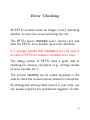
Error Checking
All PETSc routines return an integer (ierr) indicating
whether an error has occurred during the call.
The PETSc macro CHKERRQ(ierr) checks ierr and
calls the PETSc error handler upon error detection.
It is strongly advised that CHKERRQ(ierr) be used in
all calls to PETSc to enable a complete error trace.
The debug version of PETSc does a great deal of
checking for memory corruption (e.g., writing outside
of array bounds, etc.).
The macros CHKMEMQ can be called anywhere in the
code to check the current memory status for corruption.
By strategically placing these macros in your code, you
can usually pinpoint any problematic segment of code.
38
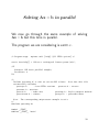
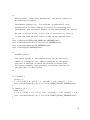
Solving Ax = b in parallel
We now go through the same example of solving
Ax = b but this time in parallel.
The program we are considering is ex23.c.
/* Program usage:
mpiexec ex23 [-help] [all PETSc options] */
static char help[] = "Solves a tridiagonal linear system.\n\n";
/*T
Concepts: KSP basic parallel example;
Processors: n
T*/
/*
Include "petscksp.h" so that we can use KSP solvers. Note that this file
automatically includes:
petscsys.h
- base PETSc routines
petscvec.h - vectors
petscmat.h - matrices
petscis.h
- index sets
petscksp.h - Krylov subspace methods
petscviewer.h - viewers
petscpc.h - preconditioners
Note:
The corresponding uniprocessor example is ex1.c
*/
#include <petscksp.h>
#undef __FUNCT__
#define __FUNCT__ "main"
39
int main(int argc,char **args)
{
Vec
x, b, u;
/* approx solution, RHS, exact solution */
Mat
A;
/* linear system matrix */
KSP
ksp;
/* linear solver context */
PC
pc;
/* preconditioner context */
PetscReal
norm,tol=1.e-11; /* norm of solution error */
PetscErrorCode ierr;
PetscInt
i,n = 10,col[3],its,rstart,rend,nlocal;
PetscScalar
neg_one = -1.0,one = 1.0,value[3];
PetscInitialize(&argc,&args,(char *)0,help);
ierr = PetscOptionsGetInt(PETSC_NULL,"-n",&n,PETSC_NULL);CHKERRQ(ierr);
/* - - - - - - - - - - - - - - - - - - - - - - - - - - - - - - - - - Compute the matrix and right-hand-side vector that define
the linear system, Ax = b.
- - - - - - - - - - - - - - - - - - - - - - - - - - - - - - - - - - */
/*
Create vectors. Note that we form 1 vector from scratch and
then duplicate as needed. For this simple case let PETSc decide how
many elements of the vector are stored on each processor. The second
argument to VecSetSizes() below causes PETSc to decide.
*/
ierr
ierr
ierr
ierr
ierr
=
=
=
=
=
VecCreate(PETSC_COMM_WORLD,&x);CHKERRQ(ierr);
VecSetSizes(x,PETSC_DECIDE,n);CHKERRQ(ierr);
VecSetFromOptions(x);CHKERRQ(ierr);
VecDuplicate(x,&b);CHKERRQ(ierr);
VecDuplicate(x,&u);CHKERRQ(ierr);
/* Identify the starting and ending mesh points on each
processor for the interior part of the mesh. We let PETSc decide
above. */
ierr = VecGetOwnershipRange(x,&rstart,&rend);CHKERRQ(ierr);
ierr = VecGetLocalSize(x,&nlocal);CHKERRQ(ierr);
40
/*
Create matrix. When using MatCreate(), the matrix format can
be specified at runtime.
Performance tuning note: For problems of substantial size,
preallocation of matrix memory is crucial for attaining good
performance. See the matrix chapter of the users manual for details.
We pass in nlocal as the "local" size of the matrix to force it
to have the same parallel layout as the vector created above.
*/
ierr
ierr
ierr
ierr
=
=
=
=
MatCreate(PETSC_COMM_WORLD,&A);CHKERRQ(ierr);
MatSetSizes(A,nlocal,nlocal,n,n);CHKERRQ(ierr);
MatSetFromOptions(A);CHKERRQ(ierr);
MatSetUp(A);CHKERRQ(ierr);
/*
Assemble matrix.
The linear system is distributed across the processors by
chunks of contiguous rows, which correspond to contiguous
sections of the mesh on which the problem is discretized.
For matrix assembly, each processor contributes entries for
the part that it owns locally.
*/
if (!rstart) {
rstart = 1;
i = 0; col[0] = 0; col[1] = 1; value[0] = 2.0; value[1] = -1.0;
ierr = MatSetValues(A,1,&i,2,col,value,INSERT_VALUES);CHKERRQ(ierr);
}
if (rend == n) {
rend = n-1;
i = n-1; col[0] = n-2; col[1] = n-1; value[0] = -1.0; value[1] = 2.0;
ierr = MatSetValues(A,1,&i,2,col,value,INSERT_VALUES);CHKERRQ(ierr);
}
41
/* Set entries corresponding to the mesh interior */
value[0] = -1.0; value[1] = 2.0; value[2] = -1.0;
for (i=rstart; i<rend; i++) {
col[0] = i-1; col[1] = i; col[2] = i+1;
ierr = MatSetValues(A,1,&i,3,col,value,INSERT_VALUES);CHKERRQ(ierr);
}
/* Assemble the matrix */
ierr = MatAssemblyBegin(A,MAT_FINAL_ASSEMBLY);CHKERRQ(ierr);
ierr = MatAssemblyEnd(A,MAT_FINAL_ASSEMBLY);CHKERRQ(ierr);
/*
Set exact solution; then compute right-hand-side vector.
*/
ierr = VecSet(u,one);CHKERRQ(ierr);
ierr = MatMult(A,u,b);CHKERRQ(ierr);
/* - - - - - - - - - - - - - - - - - - - - - - - - - - - - - - - - - Create the linear solver and set various options
- - - - - - - - - - - - - - - - - - - - - - - - - - - - - - - - - - */
/*
Create linear solver context
*/
ierr = KSPCreate(PETSC_COMM_WORLD,&ksp);CHKERRQ(ierr);
/*
Set operators. Here the matrix that defines the linear system
also serves as the preconditioning matrix.
*/
ierr = KSPSetOperators(ksp,A,A,DIFFERENT_NONZERO_PATTERN);CHKERRQ(ierr);
/*
Set linear solver defaults for this problem (optional).
- By extracting the KSP and PC contexts from the KSP context,
we can then directly call any KSP and PC routines to set
various options.
- The following four statements are optional; all of these
parameters could alternatively be specified at runtime via
42
KSPSetFromOptions();
*/
ierr = KSPGetPC(ksp,&pc);CHKERRQ(ierr);
ierr = PCSetType(pc,PCJACOBI);CHKERRQ(ierr);
ierr = KSPSetTolerances(ksp,1.e-7,PETSC_DEFAULT,PETSC_DEFAULT,PETSC_DEFAULT);
CHKERRQ(ierr);
/*
Set runtime options, e.g.,
-ksp_type <type> -pc_type <type> -ksp_monitor -ksp_rtol <rtol>
These options will override those specified above as long as
KSPSetFromOptions() is called _after_ any other customization
routines.
*/
ierr = KSPSetFromOptions(ksp);CHKERRQ(ierr);
/* - - - - - - - - - - - - - - - - - - - - - - - - - - - - - - - - - Solve the linear system
- - - - - - - - - - - - - - - - - - - - - - - - - - - - - - - - - - */
/*
Solve linear system
*/
ierr = KSPSolve(ksp,b,x);CHKERRQ(ierr);
/*
View solver info; we could instead use the option -ksp_view to
print this info to the screen at the conclusion of KSPSolve().
*/
ierr = KSPView(ksp,PETSC_VIEWER_STDOUT_WORLD);CHKERRQ(ierr);
/* - - - - - - - - - - - - - - - - - - - - - - - - - - - - - - - - - Check solution and clean up
- - - - - - - - - - - - - - - - - - - - - - - - - - - - - - - - - - */
/*
Check the error
*/
ierr = VecAXPY(x,neg_one,u);CHKERRQ(ierr);
ierr = VecNorm(x,NORM_2,&norm);CHKERRQ(ierr);
43
ierr = KSPGetIterationNumber(ksp,&its);CHKERRQ(ierr);
if (norm > tol){
ierr = PetscPrintf(PETSC_COMM_WORLD,"Norm of error %G, Iterations %D\n",norm,its);C
}
/*
Free work space. All PETSc objects should be destroyed when they
are no longer needed.
*/
ierr = VecDestroy(&x);CHKERRQ(ierr); ierr = VecDestroy(&u);CHKERRQ(ierr);
ierr = VecDestroy(&b);CHKERRQ(ierr); ierr = MatDestroy(&A);CHKERRQ(ierr);
ierr = KSPDestroy(&ksp);CHKERRQ(ierr);
/*
Always call PetscFinalize() before exiting a program. This routine
- finalizes the PETSc libraries as well as MPI
- provides summary and diagnostic information if certain runtime
options are chosen (e.g., -log_summary).
*/
ierr = PetscFinalize();
return 0;
}
44
Solving Ax = b in parallel
It is significant to realize that serial and parallel code
can look the same; the behaviour changes based on
the definition of the communicator.
In practice, there are some things to keep in mind:
• The creation routines are collective over all processes
in the communicator; thus, all processes in the
communicator must call the creation routine.
• Any sequence of collective routines must be called
in the same order on each process.
• It is possible to have finer control over matrix /
vector distribution in the parallel version.
45
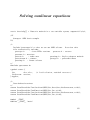
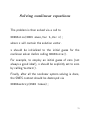
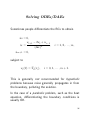
Solving nonlinear equations
It is also possible to specify and solve systems of
nonlinear algebraic equations in PETSc.
Systems of nonlinear algebraic equations take the form
F(x) = 0,
where F : <m → <m is the nonlinear residual function,
x ∈ <m is the vector of unknowns, and 0 is a vector
of zeros.
Notes:
• There may a unique solution, multiple solutions, or
no solution.
• Analysis of existence and uniqueness of solutions is
generally difficult, but especially for large m.
• Finding a suitable initial guess can also be difficult.
46
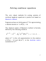
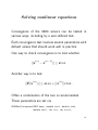
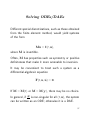
Solving nonlinear equations
The only robust methods for solving systems of
nonlinear algebraic equations in practice are based on
Newton’s method.
Suppose we have an initial guess x(0) for approximating
a desired solution x∗ to F(x) = 0.
The classical version of Newton’s method is formally
defined by the following iteration:
(n)
x(n+1) = x(n) − J−1
)F(x(n)), n = 0, 1, 2, . . . ,
F (x
where x(n) is the nth approximation to the solution
of F(x) = 0 and JF(x(n)) is the Jacobian matrix
evaluated at x(n).
47
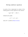
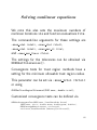
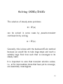
Solving nonlinear equations
In practice, this is implemented via solution of the
following system of linear equations at each iteration
JF(x(n))d(n) = −F(x(n)),
followed by the update
x(n+1) = x(n) + d(n),
where d(n) is called the Newton direction.
48
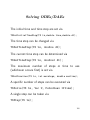
Solving nonlinear equations
In order for Newton’s method to be practical, we need
• a termination criterion that ensures a sufficiently
accurate approximate solution,
• an efficient linear system solver to compute the
Newton direction d(n),
• a globalization strategy to aid the convergence of
the iteration to a solution of F(x) = 0 for any x(0).
49
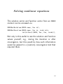
Solving nonlinear equations
In practice, a choice must be made as to how accurately
to solve for d(n).
• When x(n) is far from the solution, d(n) may not
be useful, so it may not make sense to solve for it
accurately. If you do, that is called oversolving.
• When x(n) is close to the solution, d(n) may
be useful, so it may make sense to solve for it
accurately. If you do not, that is called undersolving.
A balance between these undesirable extremes is
achieved through the use of a dynamic variable called
the forcing term, η (n).
50
Solving nonlinear equations
• Compute the Newton direction d(n) that satisfies
the inexact Newton condition
||LF(x(n))|| ≤ η (n)||F(x(n))||,
where LF(x(n)) := F(x(n)) + JF(x(n))d(n) is called
the local linear model.
• We assume that LF(x(n)) closely approximates
F(x(n+1)).
• The inexact Newton condition requires that
||LF(x(n))|| be smaller than ||F(x(n))|| by a factor
of η (n).
51
Solving nonlinear equations
• η (n) controls the level of accuracy of d(n)
– In the case of direct methods, η (n) ≡ 0; the
inexact Newton condition holds with equality.
– In the case of iterative methods, η (n) determines
the number of inner iterations to be performed.
• η (n) influences the rate of convergence and
performance of Newton’s method.
– If LF(x(n)) approximates F(x(n+1)) poorly,
choosing η (n) too small imposes too much
accuracy on d(n), thus leading to oversolving.
– Choosing η (n) too large may fail to approximate
a sufficiently accurate d(n), thus leading to
undersolving.
Oversolving or undersolving may result in little or no
reduction in the residual!
52
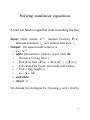
Solving nonlinear equations
A practical Newton algorithm looks something like this:
Input: initial iterate x(0), residual function F(x),
absolute tolerance τa, and relative tolerance τr .
Output: the approximate solution x
(0)
1: x ← x
2: while (termination criterion is not met) do
3:
Choose a forcing term η.
4:
Find d so that ||F(x) + JF(x)d|| ≤ η||F(x)||.
5:
If d cannot be found, terminate with failure.
6:
Find a step length λ.
7:
x ← x + λd
8: end while
9: return x
We discuss the strategies for choosing η and λ shortly.
53
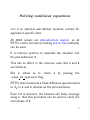
Solving nonlinear equations
The suite of routines for solving systems of nonlinear
algebraic equations in PETSc is called SNES.
In the simplest usage of SNES, the user merely provides
a C, C++, or Fortran routine to evaluate F(x).
By default, the corresponding Jacobian matrix can be
approximated with finite differences.
For improved efficiency and robustness, the user can
provide a routine to compute the Jacobian analytically
or call an automatic differentiation package.
The user has available a well-trusted forcing-term
strategy due to Eisenstat and Walker; line search or
trust region methods as globalization strategies; all
the KSP methods and preconditioners for solving linear
systems; and a modified Newton method strategy for
updating the Jacobian.
For most options, including for the termination
criterion, users are free to define their own functions.
54
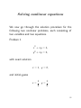
Solving nonlinear equations
We now go through the solution procedure for the
following two nonlinear problems, each consisting of
two variables and two equations.
Problem 1
x2 + xy = 3,
y 2 + xy = 6,
with exact solution
x = 1, y = 2,
and initial guess
1
1
x= , y= .
2
2
55
Solving nonlinear equations
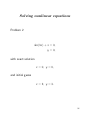
Problem 2
sin(3x) + x = 0,
y = 0,
with exact solution
x = 0, y = 0,
and initial guess
x = 2, y = 3.
56
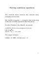
Solving nonlinear equations
The nonlinear solver directory also contains many
examples and tutorials.
We consider ex1 snes.c, a program that solves each
of the two nonlinear equations described above.
To solve Problem 1 (by default), we execute
cd $PETSC DIR/src/snes/examples/tutorials
make ex1 snes
mpiexec -np 1 ./ex1_snes
The output is simply
number of SNES iterations = 6
57
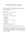
Solving nonlinear equations
To make it more informative, we can add negate the
flag in line 147 to view the complete solution:
if (!flg){
Vec f;
ierr = VecView(x,PETSC_VIEWER_STDOUT_WORLD);CHKERRQ(ierr);
ierr = SNESGetFunction(snes,&f,0,0);CHKERRQ(ierr);
ierr = VecView(r,PETSC_VIEWER_STDOUT_WORLD);CHKERRQ(ierr);
}
The (default) output is then
Vector Object: 1 MPI processes
type: seq
1
2
Vector Object: 1 MPI processes
type: seq
-4.44089e-16
0
number of SNES iterations = 6
58
Solving nonlinear equations
We solve Problem 2 by including the flag -hard when
the executable file is run:
make ex1_snes
mpiexec -np 1 ./ex1_snes -hard
This gives the output:
Vector Object: 1 MPI processes
type: seq
-2.58086e-13
-3.87421e-16
Vector Object: 1 MPI processes
type: seq
-1.03234e-12
-3.87421e-16
number of SNES iterations = 6
Note that this example does not work with np > 1.
A peculiarity of the code however is that it only reports
an error when trying to solve Problem 2; when trying
to solve Problem 1 with np > 1, it simply returns an
incorrect answer!
59
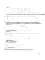
Solving nonlinear equations
static char help[] = "Newton’s method for a two-variable system, sequential.\n\n";
/*T
Concepts: SNES basic example
T*/
/*
Include "petscsnes.h" so that we can use SNES solvers. Note that this
file automatically includes:
petscsys.h
- base PETSc routines
petscvec.h - vectors
petscmat.h - matrices
petscis.h
- index sets
petscksp.h - Krylov subspace methods
petscviewer.h - viewers
petscpc.h - preconditioners
petscksp.h
- linear solvers
*/
#include <petscsnes.h>
typedef struct {
Vec
xloc,rloc;
VecScatter scatter;
} AppCtx;
/* local solution, residual vectors */
/*
User-defined routines
*/
extern
extern
extern
extern
PetscErrorCode
PetscErrorCode
PetscErrorCode
PetscErrorCode
FormJacobian1(SNES,Vec,Mat*,Mat*,MatStructure*,void*);
FormFunction1(SNES,Vec,Vec,void*);
FormJacobian2(SNES,Vec,Mat*,Mat*,MatStructure*,void*);
FormFunction2(SNES,Vec,Vec,void*);
#undef __FUNCT__
#define __FUNCT__ "main"
60
int main(int argc,char **argv)
{
SNES
snes;
/* nonlinear solver context */
KSP
ksp;
/* linear solver context */
PC
pc;
/* preconditioner context */
Vec
x,r;
/* solution, residual vectors */
Mat
J;
/* Jacobian matrix */
PetscErrorCode ierr;
PetscInt
its;
PetscMPIInt
size,rank;
PetscScalar
pfive = .5,*xx;
PetscBool
flg;
AppCtx
user;
/* user-defined work context */
IS
isglobal,islocal;
PetscInitialize(&argc,&argv,(char *)0,help);
ierr = MPI_Comm_size(PETSC_COMM_WORLD,&size);CHKERRQ(ierr);
ierr = MPI_Comm_rank(PETSC_COMM_WORLD,&rank);CHKERRQ(ierr);
/* - - - - - - - - - - - - - - - - - - - - - - - - - - - - - - - - - Create nonlinear solver context
- - - - - - - - - - - - - - - - - - - - - - - - - - - - - - - - - - */
ierr = SNESCreate(PETSC_COMM_WORLD,&snes);CHKERRQ(ierr);
/* - - - - - - - - - - - - - - - - - - - - - - - - - - - - - - - - - - Create matrix and vector data structures; set corresponding routines
- - - - - - - - - - - - - - - - - - - - - - - - - - - - - - - - - - - */
/*
Create vectors for solution and nonlinear function
*/
ierr = VecCreate(PETSC_COMM_WORLD,&x);CHKERRQ(ierr);
ierr = VecSetSizes(x,PETSC_DECIDE,2);CHKERRQ(ierr);
ierr = VecSetFromOptions(x);CHKERRQ(ierr);
ierr = VecDuplicate(x,&r);CHKERRQ(ierr);
if (size > 1){
ierr = VecCreateSeq(PETSC_COMM_SELF,2,&user.xloc);CHKERRQ(ierr);
ierr = VecDuplicate(user.xloc,&user.rloc);CHKERRQ(ierr);
61
/* Create the scatter between the global x and local xloc */
ierr = ISCreateStride(MPI_COMM_SELF,2,0,1,&islocal);CHKERRQ(ierr);
ierr = ISCreateStride(MPI_COMM_SELF,2,0,1,&isglobal);CHKERRQ(ierr);
ierr = VecScatterCreate(x,isglobal,user.xloc,islocal,&user.scatter);CHKERRQ(ierr);
ierr = ISDestroy(&isglobal);CHKERRQ(ierr);
ierr = ISDestroy(&islocal);CHKERRQ(ierr);
}
/*
Create Jacobian matrix data structure
*/
ierr = MatCreate(PETSC_COMM_WORLD,&J);CHKERRQ(ierr);
ierr = MatSetSizes(J,PETSC_DECIDE,PETSC_DECIDE,2,2);CHKERRQ(ierr);
ierr = MatSetFromOptions(J);CHKERRQ(ierr);
ierr = MatSetUp(J);CHKERRQ(ierr);
ierr = PetscOptionsHasName(PETSC_NULL,"-hard",&flg);CHKERRQ(ierr);
if (!flg) {
/*
Set function evaluation routine and vector.
*/
ierr = SNESSetFunction(snes,r,FormFunction1,&user);CHKERRQ(ierr);
/*
Set Jacobian matrix data structure and Jacobian evaluation routine
*/
ierr = SNESSetJacobian(snes,J,J,FormJacobian1,PETSC_NULL);CHKERRQ(ierr);
} else {
if (size != 1) SETERRQ(PETSC_COMM_SELF,1,"This case is a uniprocessor example only!
ierr = SNESSetFunction(snes,r,FormFunction2,PETSC_NULL);CHKERRQ(ierr);
ierr = SNESSetJacobian(snes,J,J,FormJacobian2,PETSC_NULL);CHKERRQ(ierr);
}
/* - - - - - - - - - - - - - - - - - - - - - - - - - - - - - - - - - Customize nonlinear solver; set runtime options
- - - - - - - - - - - - - - - - - - - - - - - - - - - - - - - - - - - */
/*
62
Set linear solver defaults for this problem. By extracting the
KSP, KSP, and PC contexts from the SNES context, we can then
directly call any KSP, KSP, and PC routines to set various options.
*/
ierr
ierr
ierr
ierr
=
=
=
=
SNESGetKSP(snes,&ksp);CHKERRQ(ierr);
KSPGetPC(ksp,&pc);CHKERRQ(ierr);
PCSetType(pc,PCNONE);CHKERRQ(ierr);
KSPSetTolerances(ksp,1.e-4,PETSC_DEFAULT,PETSC_DEFAULT,20);CHKERRQ(ierr);
/*
Set SNES/KSP/KSP/PC runtime options, e.g.,
-snes_view -snes_monitor -ksp_type <ksp> -pc_type <pc>
These options will override those specified above as long as
SNESSetFromOptions() is called _after_ any other customization
routines.
*/
ierr = SNESSetFromOptions(snes);CHKERRQ(ierr);
/* - - - - - - - - - - - - - - - - - - - - - - - - - - - - - - - - - Evaluate initial guess; then solve nonlinear system
- - - - - - - - - - - - - - - - - - - - - - - - - - - - - - - - - - - */
if (!flg) {
ierr = VecSet(x,pfive);CHKERRQ(ierr);
} else {
ierr = VecGetArray(x,&xx);CHKERRQ(ierr);
xx[0] = 2.0; xx[1] = 3.0;
ierr = VecRestoreArray(x,&xx);CHKERRQ(ierr);
}
/*
Note: The user should initialize the vector, x, with the initial guess
for the nonlinear solver prior to calling SNESSolve(). In particular,
to employ an initial guess of zero, the user should explicitly set
this vector to zero by calling VecSet().
*/
ierr = SNESSolve(snes,PETSC_NULL,x);CHKERRQ(ierr);
ierr = SNESGetIterationNumber(snes,&its);CHKERRQ(ierr);
if (flg) {
63
Vec f;
ierr = VecView(x,PETSC_VIEWER_STDOUT_WORLD);CHKERRQ(ierr);
ierr = SNESGetFunction(snes,&f,0,0);CHKERRQ(ierr);
ierr = VecView(r,PETSC_VIEWER_STDOUT_WORLD);CHKERRQ(ierr);
}
ierr = PetscPrintf(PETSC_COMM_WORLD,"number of SNES iterations = %D\n",its);CHKERRQ(i
/* - - - - - - - - - - - - - - - - - - - - - - - - - - - - - - - - - Free work space. All PETSc objects should be destroyed when they
are no longer needed.
- - - - - - - - - - - - - - - - - - - - - - - - - - - - - - - - - - - */
ierr = VecDestroy(&x);CHKERRQ(ierr); ierr = VecDestroy(&r);CHKERRQ(ierr);
ierr = MatDestroy(&J);CHKERRQ(ierr); ierr = SNESDestroy(&snes);CHKERRQ(ierr);
if (size > 1){
ierr = VecDestroy(&user.xloc);CHKERRQ(ierr);
ierr = VecDestroy(&user.rloc);CHKERRQ(ierr);
ierr = VecScatterDestroy(&user.scatter);CHKERRQ(ierr);
}
ierr = PetscFinalize();
return 0;
}
/* ------------------------------------------------------------------- */
#undef __FUNCT__
#define __FUNCT__ "FormFunction1"
/*
FormFunction1 - Evaluates nonlinear function, F(x).
.
.
.
Input Parameters:
snes - the SNES context
x
- input vector
ctx - optional user-defined context
Output Parameter:
f - function vector
.
*/
PetscErrorCode FormFunction1(SNES snes,Vec x,Vec f,void *ctx)
64
{
PetscErrorCode
const PetscScalar
PetscScalar
AppCtx
Vec
VecScatter
MPI_Comm
PetscMPIInt
PetscInt
ierr;
*xx;
*ff;
*user = (AppCtx*)ctx;
xloc=user->xloc,floc=user->rloc;
scatter=user->scatter;
comm;
size,rank;
rstart,rend;
ierr = PetscObjectGetComm((PetscObject)snes,&comm);CHKERRQ(ierr);
ierr = MPI_Comm_size(comm,&size);CHKERRQ(ierr);
ierr = MPI_Comm_rank(comm,&rank);CHKERRQ(ierr);
if (size > 1){
/*
This is a ridiculous case for testing intermidiate steps from sequential
code development to parallel implementation.
(1) scatter x into a sequetial vector;
(2) each process evaluates all values of floc;
(3) scatter floc back to the parallel f.
*/
ierr = VecScatterBegin(scatter,x,xloc,INSERT_VALUES,SCATTER_FORWARD);CHKERRQ(ierr);
ierr = VecScatterEnd(scatter,x,xloc,INSERT_VALUES,SCATTER_FORWARD);CHKERRQ(ierr);
ierr = VecGetOwnershipRange(f,&rstart,&rend);CHKERRQ(ierr);
ierr = VecGetArrayRead(xloc,&xx);CHKERRQ(ierr);
ierr = VecGetArray(floc,&ff);CHKERRQ(ierr);
ff[0] = xx[0]*xx[0] + xx[0]*xx[1] - 3.0;
ff[1] = xx[0]*xx[1] + xx[1]*xx[1] - 6.0;
ierr = VecRestoreArray(floc,&ff);CHKERRQ(ierr);
ierr = VecRestoreArrayRead(xloc,&xx);CHKERRQ(ierr);
ierr
ierr
} else
/*
Get
= VecScatterBegin(scatter,floc,f,INSERT_VALUES,SCATTER_REVERSE);CHKERRQ(ierr);
= VecScatterEnd(scatter,floc,f,INSERT_VALUES,SCATTER_REVERSE);CHKERRQ(ierr);
{
pointers to vector data.
65
- For
the
- You
the
default PETSc vectors, VecGetArray() returns a pointer to
data array. Otherwise, the routine is implementation dependent.
MUST call VecRestoreArray() when you no longer need access to
array.
*/
ierr = VecGetArrayRead(x,&xx);CHKERRQ(ierr);
ierr = VecGetArray(f,&ff);CHKERRQ(ierr);
/* Compute function */
ff[0] = xx[0]*xx[0] + xx[0]*xx[1] - 3.0;
ff[1] = xx[0]*xx[1] + xx[1]*xx[1] - 6.0;
/* Restore vectors */
ierr = VecRestoreArrayRead(x,&xx);CHKERRQ(ierr);
ierr = VecRestoreArray(f,&ff);CHKERRQ(ierr);
}
return 0;
}
/* ------------------------------------------------------------------- */
#undef __FUNCT__
#define __FUNCT__ "FormJacobian1"
/*
FormJacobian1 - Evaluates Jacobian matrix.
.
.
.
Input Parameters:
snes - the SNES context
x - input vector
dummy - optional user-defined context (not used here)
Output Parameters:
. jac - Jacobian matrix
. B - optionally different preconditioning matrix
. flag - flag indicating matrix structure
*/
PetscErrorCode FormJacobian1(SNES snes,Vec x,Mat *jac,Mat *B,MatStructure *flag,void *d
{
PetscScalar
*xx,A[4];
PetscErrorCode ierr;
66
PetscInt
idx[2] = {0,1};
/*
Get pointer to vector data
*/
ierr = VecGetArray(x,&xx);CHKERRQ(ierr);
/*
Compute Jacobian entries and insert into matrix.
- Since this is such a small problem, we set all entries for
the matrix at once.
*/
A[0] = 2.0*xx[0] + xx[1]; A[1] = xx[0];
A[2] = xx[1]; A[3] = xx[0] + 2.0*xx[1];
ierr = MatSetValues(*B,2,idx,2,idx,A,INSERT_VALUES);CHKERRQ(ierr);
*flag = SAME_NONZERO_PATTERN;
/*
Restore vector
*/
ierr = VecRestoreArray(x,&xx);CHKERRQ(ierr);
/*
Assemble matrix
*/
ierr = MatAssemblyBegin(*B,MAT_FINAL_ASSEMBLY);CHKERRQ(ierr);
ierr = MatAssemblyEnd(*B,MAT_FINAL_ASSEMBLY);CHKERRQ(ierr);
if (*jac != *B){
ierr = MatAssemblyBegin(*jac,MAT_FINAL_ASSEMBLY);CHKERRQ(ierr);
ierr = MatAssemblyEnd(*jac,MAT_FINAL_ASSEMBLY);CHKERRQ(ierr);
}
return 0;
}
/* ------------------------------------------------------------------- */
#undef __FUNCT__
#define __FUNCT__ "FormFunction2"
PetscErrorCode FormFunction2(SNES snes,Vec x,Vec f,void *dummy)
67
{
PetscErrorCode ierr;
PetscScalar
*xx,*ff;
/*
Get pointers to vector data.
- For default PETSc vectors, VecGetArray() returns a pointer to
the data array. Otherwise, the routine is implementation dependent.
- You MUST call VecRestoreArray() when you no longer need access to
the array.
*/
ierr = VecGetArray(x,&xx);CHKERRQ(ierr);
ierr = VecGetArray(f,&ff);CHKERRQ(ierr);
/*
Compute function
*/
ff[0] = PetscSinScalar(3.0*xx[0]) + xx[0];
ff[1] = xx[1];
/*
Restore vectors
*/
ierr = VecRestoreArray(x,&xx);CHKERRQ(ierr);
ierr = VecRestoreArray(f,&ff);CHKERRQ(ierr);
return 0;
}
/* ------------------------------------------------------------------- */
#undef __FUNCT__
#define __FUNCT__ "FormJacobian2"
PetscErrorCode FormJacobian2(SNES snes,Vec x,Mat *jac,Mat *B,MatStructure *flag,void *d
{
PetscScalar
*xx,A[4];
PetscErrorCode ierr;
PetscInt
idx[2] = {0,1};
/*
Get pointer to vector data
68
*/
ierr = VecGetArray(x,&xx);CHKERRQ(ierr);
/*
Compute Jacobian entries and insert into matrix.
- Since this is such a small problem, we set all entries for
the matrix at once.
*/
A[0] = 3.0*PetscCosScalar(3.0*xx[0]) + 1.0; A[1] = 0.0;
A[2] = 0.0;
A[3] = 1.0;
ierr = MatSetValues(*B,2,idx,2,idx,A,INSERT_VALUES);CHKERRQ(ierr);
*flag = SAME_NONZERO_PATTERN;
/*
Restore vector
*/
ierr = VecRestoreArray(x,&xx);CHKERRQ(ierr);
/*
Assemble matrix
*/
ierr = MatAssemblyBegin(*B,MAT_FINAL_ASSEMBLY);CHKERRQ(ierr);
ierr = MatAssemblyEnd(*B,MAT_FINAL_ASSEMBLY);CHKERRQ(ierr);
if (*jac != *B){
ierr = MatAssemblyBegin(*jac,MAT_FINAL_ASSEMBLY);CHKERRQ(ierr);
ierr = MatAssemblyEnd(*jac,MAT_FINAL_ASSEMBLY);CHKERRQ(ierr);
}
return 0;
}
69
Solving nonlinear equations
Notes:
• An SNES solver is created via a call of the form
SNESCreate(MPI Comm comm,SNES *snes);
• The routines to evaluate F(x) and JF(x) are set.
• The nonlinear solution method is chosen via
SNESSetType(SNES snes,SNESType method);
or from command line via
-snes_type <method>
70
Solving nonlinear equations
An application code can take complete control of the
solvers (both linear and nonlinear) via
SNESSetFromOptions(snes);
This function provides an interface to the PETSc
options database so that choices can be made at
runtime for things such as the
• particular nonlinear solver,
• various parameters and customized routines, e.g.,
specialized line search variants,
• convergence tolerance,
• monitoring routines,
• linear solver options in the KSP and PC modules.
71
Solving nonlinear equations
The problem is then solved via a call to
SNESSolve(SNES snes,Vec b,Vec x);
where x will contain the solution vector.
x should be initialized to the initial guess for the
nonlinear solver before calling SNESSolve().
For example, to employ an initial guess of zero (not
always a good idea!), x should be explicitly set to zero
by calling VecSet().
Finally, after all the nonlinear system solving is done,
the SNES context should be destroyed via
SNESDestroy(SNES *snes);
72
Solving nonlinear equations
The user specifies the system of nonlinear equations
F(x) = 0 to be solved via
SNESSetFunction(SNES snes,Vec f,
PetscErrorCode (*FormFunction)(SNES snes,Vec x,Vec f,void *ctx),void *ctx);
The argument ctx is an optional user-defined context
that can store any private, application-specific data
required by the function evaluation routine.
Use PETSC NULL if such information is not needed.
Some kind of routine to approximate JF(x) is typically
specified with
SNESSetJacobian(SNES snes,Mat A,Mat B,PetscErrorCode (*FormJacobian)(SNES snes,
Vec x,Mat *A,Mat *B,MatStructure *flag,void *ctx),void *ctx);
where x is the current iterate, A is the Jacobian
matrix, B is the preconditioner (usually =A),
flag gives information about the preconditioner
structure (identical to the options for the flag of
KSPSetOperators()).
73
Solving nonlinear equations
ctx is an optional user-defined Jacobian context for
application-specific data.
All SNES solvers are data-structure neutral, so all
PETSc matrix formats (including matrix-free methods)
can be used.
It is common practice to assemble the Jacobian into
the preconditioner B.
This has no effect in the common case that A and B
are identical.
But it allows us to check A by passing the
-snes mf operator flag.
PETSc then constructs a finite-difference approximation
to JF in A and B remains as the preconditioner.
Even if B is incorrect, the iteration will likely converge
using A; thus this procedure can be used to verify the
correctness of B.
74
Solving nonlinear equations
The globalization strategies built in to PETSc are
based on line search and trust region methods.
The method SNESLS (which can also be invoked via
the flag -snes type ls) provides a line search for
Newton’s method.
The default strategy is called cubic backtracking.
The idea of a line search is natural: given a descent
direction d(n), take a step in that direction that yields
an “acceptable” x(n+1).
The term line search refers to a procedure for finding
the step length λ.
The accepted strategy is to first try λ = 1.
If this fails to satisfy the criterion that makes x(n+1)
acceptable, then we backtrack in a systematic fashion
along d(n).
75
Solving nonlinear equations
Experience has shown the importance of taking the full
Newton step whenever possible.
Failure to do so leads to sub-optimal convergence rates
near the solution.
Although no criterion will always be optimal, it seems
to be good sense to require
||F(x(n+1))|| < ||F(x(n))||.
If we compute JF(x(n+1)) along with F(x(n+1)), then
we will have 4 pieces of information (function values
and derivatives at each of the two end-points λ = 0
and λ = 1 of the line search.
This means we can fit a cubic interpolating polynomial
to these points and find its minimizer analytically.
This value of λ is taken as the value to be used when
determining x(n+1).
76
Solving nonlinear equations
Alternative line search routines can be set via
SNESSetLineSearch(SNES snes,PetscErrorCode
(*ls)(SNES,Vec,Vec,Vec,Vec,double,double*,double*), void *lsctx);
PETSc also provides other line search methods
SNESSearchQuadraticLine(), SNESLineSearchNo(),
and SNESLineSearchNoNorms(), which can be set via
-snes_ls [cubic, quadratic, basic, basicnonorms]
where cubic is the (default) method just discussed,
quadratic is the corresponding backtracking line
search method based on a quadratic interpolant, basic
is really only a template for a classical Newton iteration,
and basicnonorms is a classical Newton iteration.
77
Solving nonlinear equations
It is not recommended to use either basic or
basicnonorms options in general.
It may make sense to use the basicnonorms option
when you know you want to perform a fixed number
of full Newton iterations.
This might be the case when trying to achieve an
efficient approximation to a solution starting from a
highly accurate initial guess.
Examples include predictor-corrector methods and
fully implicit Runge–Kutta methods for initial-value
problems and error estimators and deferred corrections
for boundary-value problems.
The line search routines involve several parameters
with defaults that are often reasonable in practice;
they can be overridden via -snes ls alpha <alpha>,
-snes ls maxstep <max>, and -snes ls steptol <tol>.
78
Solving nonlinear equations
Line search methods attempt to compute an acceptable
step length in a given search direction.
The underlying assumptions were that the direction
would be d(n) and λ = 1 would be the first trial step.
In trust region methods, we relax the assumption that
the step be in the direction d(n).
Indeed there is more information available from
JF(x(n)), and trust region methods try to use it.
Trust region methods use a pre-specified step length.
For example, it may not be so unreasonable to begin
with a step length on the order of the previous one.
The general idea is define a region in which the local
linear model approximates the actual model well and
adjust its size as the iteration proceeds.
Several effective heuristics are available for this.
79
Solving nonlinear equations
The trust region method used by SNES is invoked via
SNESTR (or the -snes type tr flag).
The strategy itself is taken from the MINPACK project.
There are several parameters that control the size of
the trust region during the solution process.
For example, the user can control the initial trust
region radius ∆ in
∆ = ∆0||F0||2
by setting ∆0 via the flag -snes tr delta0 <delta0>.
80
Solving nonlinear equations
Convergence of the SNES solvers can be tested in
various ways, including by a user-defined test.
Each convergence test involves several parameters with
default values that should work well in practice.
One way to check convergence is to test whether
||x(n) − x(n−1)|| ≤ stol.
Another way is to test
||F(x(n))|| ≤ atol + ||x(n)||rtol.
Often a combination of the two is recommended.
These parameters are set via
SNESSetTolerances(SNES snes, double atol, double rtol,
double stol, int its, int fcts);
81
Solving nonlinear equations
We note this also sets the maximum numbers of
nonlinear iterations its and function evaluations fcts.
The command-line arguments for these settings are
-snes atol <atol>, -snes rtol <rtol>,
-snes stol <stol>, -snes max it <its>,
and -snes max funcs <fcts>.
The settings for the tolerances can be obtained via
SNESGetTolerances().
Convergence tests for trust region methods have a
setting for the minimum allowable trust region radius.
This parameter can be set via -snes trtol <trtol>
or using
SNESSetTrustRegionTolerance(SNES snes, double trtol);
Customized convergence tests can be defined via
SNESSetConvergenceTest(SNES snes, PetscErrorCode (*test)
(SNES snes, int it, double xnorm, double gnorm, double f,
SNESConvergedReason reason, void *cctx),
void *cctx,PetscErrorCode (*destroy)(void *cctx));
82
Solving nonlinear equations
By default, the SNES solvers do not display information
about the iterations.
Monitoring can be established via
SNESMonitorSet(SNES snes,PetscErrorCode
(*mon)(SNES, int its, double norm, void* mctx),
void *mctx, PetscErrorCode (*monitordestroy)(void**));
where mon is a user-defined monitoring routine, its
and mctx are the iteration number and an optional
user-defined context for private data for the monitor
routine, and norm is the function norm.
SNESMonitorSet() is called once after every
(outer) SNES iteration; hence, any application-specific
computations can be done after each iteration.
The option -snes monitor activates the SNES monitor
routine SNESMonitorDefault(); -snes monitor draw
draws a simple graph of ||F(x)||.
Monitoring routines for SNES can be cancelled at
runtime via the -snes monitor cancel option.
83
Solving nonlinear equations
The solution vector and function vector from an SNES
context can be accessed via
SNESGetSolution(SNES snes, Vec *x);
SNESGetFunction(SNES snes, Vec *r, void *ctx,
int(**func)(SNES, Vec, Vec, void*));
Not only is this useful to see the solution and function
values yourself, e.g., during the iteration or after
convergence, but this would be how such information
would be passed to a (custom) convergence test that
required them.
84
Solving IVPs
PETSc can be used to solve initial-value problems
(IVPs) in ordinary differential equations (ODEs) and
differential-algebraic equations (DAEs).
Consider the following example:
dy
= −y,
dt
y(0) = 1.
First, we set up a makefile to build the executable:
#Makefile to build ode_example.c
include ${PETSC DIR}/conf/base
ode_example: ode_example.o chkopts
-${CLINKER} -o ode example ode example.o
$RM ode_example.o
${PETSC TS LIB}
85
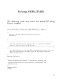
Solving ODEs/DAEs
The following code now solves the above IVP using
Euler’s method.
static char help[] ="Solves the simple ODE dy/dt=-y, y(0)=1.";
/*
Concepts: solving ordinary differential equations
Processors: 1
*/
/* -----------------------------------------------------------------------This code demonstrates how one may solve an ordinary differential
equation using the built-in ODE solvers.
--------------------------------------------------------------------- */
/*
Include "petscts.h" to use the PETSc timestepping routines. Note that
this file automatically includes "petsc.h" and other lower-level
PETSc include files.
*/
#include "petscts.h"
/*
Create an application context to contain data needed by the
application-provided call-back routines, FormJacobian() and
FormFunction().
*/
typedef struct {
} AppCtx;
86
/*
User-defined routines
*/
extern PetscErrorCode RHSFunction(TS,PetscReal,Vec,Vec,void*);
#undef __FUNCT__
#define __FUNCT__ "main"
int main(int argc,char **argv)
{
TS
ts;
Vec
y;
PetscErrorCode ierr;
PetscReal
end_time, dt;
PetscReal ftime;
PetscInt
num_time_steps;
AppCtx
user;
PetscScalar
*initial_condition;
/* timestepping context */
/* solution, residual vectors */
/* user-defined work context */
PetscInitialize(&argc,&argv,PETSC_NULL,help);
//Set up the timestep (can be an option from command line)
dt = 0.5;
end_time=1.0;
ierr = PetscOptionsGetReal(PETSC_NULL,"-dt",&dt,PETSC_NULL);CHKERRQ(ierr);
num_time_steps = round(end_time/dt);
/*
Create vector to hold the solution
*/
ierr = VecCreateSeq(PETSC_COMM_SELF,1,&y);CHKERRQ(ierr);
/*
Create timestepper context
*/
ierr = TSCreate(PETSC_COMM_WORLD,&ts);CHKERRQ(ierr);
ierr = TSSetProblemType(ts,TS_NONLINEAR);CHKERRQ(ierr);
/*
87
Set initial condition
*/
ierr = VecGetArray(y,&initial_condition);CHKERRQ(ierr);
initial_condition[0]=1.0;
ierr = VecRestoreArray(y,&initial_condition);CHKERRQ(ierr);
ierr = TSSetSolution(ts,y);CHKERRQ(ierr);
/*
Provide the call-back for the nonlinear function we are
evaluating, dy/dt=f(t,y). Thus whenever the timestepping routines
need the function they will call this routine. Note the final
argument is the application context used by the call-back functions.
*/
ierr = TSSetRHSFunction(ts, PETSC_NULL, RHSFunction,&user);CHKERRQ(ierr);
/*
This indicates that we are using Euler’s method.
*/
ierr = TSSetType(ts,TSEULER);CHKERRQ(ierr);
/*
Set the initial time and the initial timestep given above.
*/
ierr = TSSetInitialTimeStep(ts,0.0,dt);CHKERRQ(ierr);
/*
Set a maximum number of timesteps and final simulation time.
*/
ierr = TSSetDuration(ts,num_time_steps,end_time);
/*
Set any additional options from the options database. This
includes all options for the nonlinear and linear solvers used
internally the the timestepping routines.
*/
ierr = TSSetFromOptions(ts);CHKERRQ(ierr);
ierr = TSSetUp(ts);CHKERRQ(ierr);
88
/*
Perform the solve. This is where the timestepping takes place.
*/
ierr = TSSolve(ts, y, &ftime);CHKERRQ(ierr);
/*
View information about the time-stepping method and the solution
at the end time.
*/
TSView(ts, PETSC_VIEWER_STDOUT_SELF);
VecView(y, PETSC_VIEWER_STDOUT_SELF);
printf("\nThis is ftime: %f\n", ftime);
/*
Free the data structures constructed above
*/
ierr = VecDestroy(&y);CHKERRQ(ierr);
ierr = TSDestroy(&ts);CHKERRQ(ierr);
ierr = PetscFinalize();CHKERRQ(ierr);
return 0;
}
#undef __FUNCT__
#define __FUNCT__ "RHSFunction"
PetscErrorCode RHSFunction(TS ts,PetscReal t,Vec X,Vec F,void *ptr)
{
PetscErrorCode ierr;
PetscScalar
*y, *f;
ierr = VecGetArray(X,&y);CHKERRQ(ierr);
ierr = VecGetArray(F,&f);CHKERRQ(ierr);
f[0]=-y[0]; // dy/dt = -y
ierr = VecRestoreArray(X,&y);CHKERRQ(ierr);
ierr = VecRestoreArray(F,&f);CHKERRQ(ierr);
return 0;
}
89
Command-line options
It is possible to specify (non-default) methods used to
solve a problem via command-line options when the
executable is launched, e.g., the preconditioner and the
KSP solver.
It is also possible to specify that an external package
such as MUMPS be used as the linear system solver.
Additional PETSc information about the run can also
be displayed.
For example, after running the makefile to build
ex23.c, the executable can be run with the ilu
preconditioner, cg solver, and additional output,
including viewing the matrix A.
mpiexec -np 2 ./ex23 -ksp type cg -pc type ilu -log summary -mat view
The ability to change the methods used to solve a
linear system makes it convenient test a variety of
numerical methods on a given problem.
90
Solving ODEs/DAEs
Other ODE solvers are available, including the
backward Euler method, the Crank–Nicolson method,
and the solvers from the sundials package, cvode
and ida.
sundials stands for the SUite of
DIfferential-ALgebraic equation Solvers.
Nonlinear
It was developed at the Lawrence Livermore National
Laboratory, where it continues to be supported,
developed, and maintained.
cvode is a powerful general-purpose IVP solver that
includes methods for non-stiff and stiff systems.
In the case of stiff systems, the implicit solvers can
use direct (full or banded) linear system solvers for the
Newton iteration as well as iterative (preconditioned
Krylov subspace) methods.
At present, cvode contains three Krylov subspace
methods; GMRES, Bi-CGStab, and TFQMR.
91
Solving ODEs/DAEs
In general, GMRES is considered to be the most robust
solver (and hence the one to try first).
An advantage of cvode (as in PETSc) is that it is
easy to try the other Krylov space solvers if convergence
issues are encountered with GMRES.
Historically, there used to be a parallel version of
cvode called pvode, but it has been incorporated
into cvode.
The family of solvers known as sundials actually
consists of cvode for IVPs in ODEs, kinsol for
nonlinear algebraic equations, ida for IVPs in DAEs,
and the extensions cvodes and idas that can perform
sensitivity analyses (both forward and adjoint).
92
Solving ODEs/DAEs
The TS library in PETSc provides a framework for
solving ODEs and DAEs in parallel.
The main motivation is to solve such problems as
resulting from the method of lines applied to timedependent PDEs.
It is also possible to solve time-independent
(stationary/steady-state) PDEs through the use of the
method of lines combined with pseudo-timestepping.
For example, suppose a temperature distribution
u(x, t) satisfies the heat equation
ut = uxx,
a < x < b, t > 0,
subject to the boundary and initial data
u(a, t) = Ta,
u(b, t) = Tb,
u(x, 0) = T0(x).
93
Solving ODEs/DAEs
This PDE can be discretized by the method of lines on
a uniform spatial mesh with m + 1 subintervals using
centred differences for the spatial derivative to yield
the initial-value DAE
0 = u0 − Ta,
ui+1 − 2ui + ui−1
,
u̇i =
(∆x)2
i = 1, 2, . . . , m,
0 = um+1 − Tb,
subject to
ui(0) = T0(xi),
i = 0, 1, . . . , m + 1.
94
Solving ODEs/DAEs
In this case one could take advantage of the explicit
knowledge we have of the Dirichlet boundary conditions
to write the problem as an IVP for an ODE
u2 − 2u1 + Ta
u̇1 =
,
(∆x)2
ui+1 − 2ui + ui−1
,
u̇i =
2
(∆x)
Tb − 2um + um−1
u̇m =
,
(∆x)2
i = 2, 3, . . . , m − 1,
subject to
ui(0) = T0(xi),
i = 1, 2, . . . , m.
95
Solving ODEs/DAEs
Sometimes people differentiate the BCs to obtain
u̇0 = 0,
ui+1 − 2ui + ui−1
u̇i =
,
(∆x)2
i = 1, 2, . . . , m,
u̇m+1 = 0,
subject to
ui(0) = T0(xi),
i = 0, 1, . . . , m + 1.
This is generally not recommended for hyperbolic
problems because noise generally propagates in from
the boundary, polluting the solution.
In the case of a parabolic problem, such as the heat
equation, differentiating the boundary conditions is
usually OK.
96
Solving ODEs/DAEs
Different spatial discretizations, such as those obtained
from the finite element method, would yield systems
of the form
Mu̇ = f (t, u),
where M is invertible.
Often, M has properties such as symmetry or positive
definiteness that make it more amenable to inversion.
It may be convenient to treat such a system as a
differential-algebraic equation
F(t, u, u̇) = 0.
If M = M(t) or M = M(y), there may be no choice.
In general, if ∂∂Fu̇ is non-singular for all (t, u), the system
can be written as an ODE; otherwise it is a DAE.
97
Solving ODEs/DAEs
The solution of steady-state problems
0 = F(u)
can be solved in some cases by pseudo-transient
continuation by solving
u̇ = F(u).
Generally, this is done with the backward Euler method
because we would like to take large steps and reach a
suitably large final time such that u converges to its
steady state.
It is important to note that transient solution values,
i.e., at for intermediate times that have yet to converge,
are essentially meaningless.
98
Solving ODEs/DAEs
The TS library is used in a manner similar to other
libraries in PETSc.
A TS object is created with the command
int TSCreate(MPI Comm comm, TSProblemType problemtype, TS *ts);
The TSProblemType is set to TS LINEAR if u̇ = A(t)u
or TS NONLINEAR if u̇ = F(t, u).
The solution method is set via
TSSetType(TS ts, TSType type);
where the supported types are TSEULER, TSRK
(Runge–Kutta), TSBEULER, TSCN (Crank–Nicolson),
TSTHETA, TSGL (generalized linear), TSPSEUDO, and
TSSUNDIALS (if the Sundials package is installed),
or the command-line option -ts type euler, rk,
beuler, cn, theta, gl, pseudo, sundials.
Normally, it is best to use the TSSetFromOptions()
command and then set the TS type from the options
database rather than by using this routine.
99
Solving ODEs/DAEs
The initial time and time step are set via
TSSetInitialTimeStep(TS ts,double time,double dt);
The time step can be changed via
TSSetTimeStep(TS ts, double dt);
The current time step can be determined via
TSGetTimeStep(TS ts, double* dt);
The maximum number of steps or time to use
(whichever occurs first) is set via
TSSetDuration(TS ts, int maxsteps, double maxtime);
A specific number of steps can be executed via
TSSolve(TS ts, Vec U, PetscReal *ftime);
A single step can be taken via
TSStep(TS ts);
100
Solving ODEs/DAEs
The TSSolve call implicitly sets up the timestep
context, but it can be done explicitly with
TSSetUp(TS ts);
The context can be viewed via
TSView(TS ts, PetscViewer viewer);
and destroyed via
TSDestroy(TS *ts);
Initial conditions are set via
TSSetSolution(TS ts, Vec initialsolution);
101
Solving ODEs/DAEs
The right-hand side function for ODEs is set according
to whether it is linear and an implicit solver is being
used.
Linear functions solved with an implicit solver are
invoked via
TSSetMatrices(TS ts,
Mat A, PetscErrorCode (*frhs)(TS, PetscReal, Mat*, Mat*, MatStructure*, void*),
Mat B, PetscErrorCode (*flhs)(TS, PetscReal, Mat*, Mat*, MatStructure*, void*),
MatStructure flag,void *ctx)
where the solver is assumed to take the form
Bun+1 = Aun.
The functions frhs and flhs are used to form A and
B at each time step if they are time dependent.
If not, the user should pass in PETSC NULL.
102
Solving ODEs/DAEs
The variable ctx allows users to pass in an application
context that is passed to the frhs() or flhs()
function, whenever they are called, as the final
argument.
The user must provide the matrix A.
If B= I, the user should pass in PETSC NULL.
If the right-hand side is provided only as a linear
function, the user must construct a MATSHELL matrix
shell to provide a user-defined matrix type.
We note that this is the same interface as that for
SNESSetJacobian().
103
Solving ODEs/DAEs
The right-hand side for nonlinear problems or linear
problems solved using explicit methods is set up via
TSSetRHSFunction(TS ts, Vec R,
PetscErrorCode (*f)(TS, double, Vec, Vec, void*), void *fP);
where the vector R is an optional location to store the
result.
The arguments to the function f() are the time step
context, the current time, the input for the function,
the output for the function, and the (optional) userprovided context variable fP.
104
Solving ODEs/DAEs
For nonlinear problems the user must also provide
the (approximate) Jacobian matrix of F(t, u) and a
function to compute it at each Newton iteration.
This is done via
TSSetRHSJacobian(TS ts, Mat A, Mat P,
PetscErrorCode (*fjac)(TS, double, Vec, Mat*, Mat*, MatStructure*, void*),
void *fP);
where the arguments for the function fjac() are the
time step context, the current time, the location where
the Jacobian is to be computed, the Jacobian matrix,
an alternative approximate Jacobian matrix used as a
preconditioner, and the optional user-provided context,
passed in as fP.
The user must provide the Jacobian as a matrix; thus,
if a matrix-free approach is used, the user must create
a MATSHELL matrix.
We again note the similarity to SNESSetJacobian().
105
Solving ODEs/DAEs
To solve a DAE, instead of TSSetRHSFunction() and
TSSetRHSJacobian(), one uses
TSSetIFunction(TS ts, Vec R,
PetscErrorCode (*f)(TS,PetscReal,Vec,Vec,Vec,void*), void *funP);
where the vector R is an optional location to store the
residual.
The arguments to f() are the time step context,
current time, input state u, input time derivative u t,
and the (optional) user-provided context funP.
106
Solving ODEs/DAEs
Unless one is using a matrix-free method without
preconditioning, the user must also provide an
(approximate) Jacobian matrix of
G(u) = F(t, u, w + au)
because the integrator internally sets u̇ ≈ w + au,
where the positive shift a and vector w depend on the
integration method, step size, and past states.
The function to evaluate G0(u) = Fu + aFu̇ is set via
TSSetIJacobian(TS ts, Mat A, Mat B,
PetscErrorCode (*fjac)(TS,PetscReal,Vec,Vec,PetscReal,Mat*,Mat*,MatStructure*,void*),
void *jacP);
where fjac() takes the time step context, current
time, input state u, input derivative u t, shift a, matrix
A, preconditioning matrix B, flag describing structure
of preconditioning matrix (see KSPSetOperators()),
and the (optional) user-provided context jacP.
107
Summary
• PETSc: scientific library used to solve applications
modelled by partial differential equations
• Large suite of sequential and parallel nonlinear and
linear algebraic equation solvers
• Used in many applications, including
simulation and carbon sequestration
heart
• One of the go-to libraries for solving large, sparse
linear systems
• MPI used for parallelization
• High-level use of MPI for users
• Easy for beginners; fine-grained control for experts
108