Download Digital Signal Processing with V850 and V850E Devices Application

To our customers,
Old Company Name in Catalogs and Other Documents
On April 1st, 2010, NEC Electronics Corporation merged with Renesas Technology
Corporation, and Renesas Electronics Corporation took over all the business of both
companies. Therefore, although the old company name remains in this document, it is a valid
Renesas Electronics document. We appreciate your understanding.
Renesas Electronics website: http://www.renesas.com
April 1st, 2010
Renesas Electronics Corporation
Issued by: Renesas Electronics Corporation (http://www.renesas.com)
Send any inquiries to http://www.renesas.com/inquiry.
Notice
1.
2.
3.
4.
5.
6.
7.
All information included in this document is current as of the date this document is issued. Such information, however, is
subject to change without any prior notice. Before purchasing or using any Renesas Electronics products listed herein, please
confirm the latest product information with a Renesas Electronics sales office. Also, please pay regular and careful attention to
additional and different information to be disclosed by Renesas Electronics such as that disclosed through our website.
Renesas Electronics does not assume any liability for infringement of patents, copyrights, or other intellectual property rights
of third parties by or arising from the use of Renesas Electronics products or technical information described in this document.
No license, express, implied or otherwise, is granted hereby under any patents, copyrights or other intellectual property rights
of Renesas Electronics or others.
You should not alter, modify, copy, or otherwise misappropriate any Renesas Electronics product, whether in whole or in part.
Descriptions of circuits, software and other related information in this document are provided only to illustrate the operation of
semiconductor products and application examples. You are fully responsible for the incorporation of these circuits, software,
and information in the design of your equipment. Renesas Electronics assumes no responsibility for any losses incurred by
you or third parties arising from the use of these circuits, software, or information.
When exporting the products or technology described in this document, you should comply with the applicable export control
laws and regulations and follow the procedures required by such laws and regulations. You should not use Renesas
Electronics products or the technology described in this document for any purpose relating to military applications or use by
the military, including but not limited to the development of weapons of mass destruction. Renesas Electronics products and
technology may not be used for or incorporated into any products or systems whose manufacture, use, or sale is prohibited
under any applicable domestic or foreign laws or regulations.
Renesas Electronics has used reasonable care in preparing the information included in this document, but Renesas Electronics
does not warrant that such information is error free. Renesas Electronics assumes no liability whatsoever for any damages
incurred by you resulting from errors in or omissions from the information included herein.
Renesas Electronics products are classified according to the following three quality grades: “Standard”, “High Quality”, and
“Specific”. The recommended applications for each Renesas Electronics product depends on the product’s quality grade, as
indicated below. You must check the quality grade of each Renesas Electronics product before using it in a particular
application. You may not use any Renesas Electronics product for any application categorized as “Specific” without the prior
written consent of Renesas Electronics. Further, you may not use any Renesas Electronics product for any application for
which it is not intended without the prior written consent of Renesas Electronics. Renesas Electronics shall not be in any way
liable for any damages or losses incurred by you or third parties arising from the use of any Renesas Electronics product for an
application categorized as “Specific” or for which the product is not intended where you have failed to obtain the prior written
consent of Renesas Electronics. The quality grade of each Renesas Electronics product is “Standard” unless otherwise
expressly specified in a Renesas Electronics data sheets or data books, etc.
“Standard”:
8.
9.
10.
11.
12.
Computers; office equipment; communications equipment; test and measurement equipment; audio and visual
equipment; home electronic appliances; machine tools; personal electronic equipment; and industrial robots.
“High Quality”: Transportation equipment (automobiles, trains, ships, etc.); traffic control systems; anti-disaster systems; anticrime systems; safety equipment; and medical equipment not specifically designed for life support.
“Specific”:
Aircraft; aerospace equipment; submersible repeaters; nuclear reactor control systems; medical equipment or
systems for life support (e.g. artificial life support devices or systems), surgical implantations, or healthcare
intervention (e.g. excision, etc.), and any other applications or purposes that pose a direct threat to human life.
You should use the Renesas Electronics products described in this document within the range specified by Renesas Electronics,
especially with respect to the maximum rating, operating supply voltage range, movement power voltage range, heat radiation
characteristics, installation and other product characteristics. Renesas Electronics shall have no liability for malfunctions or
damages arising out of the use of Renesas Electronics products beyond such specified ranges.
Although Renesas Electronics endeavors to improve the quality and reliability of its products, semiconductor products have
specific characteristics such as the occurrence of failure at a certain rate and malfunctions under certain use conditions. Further,
Renesas Electronics products are not subject to radiation resistance design. Please be sure to implement safety measures to
guard them against the possibility of physical injury, and injury or damage caused by fire in the event of the failure of a
Renesas Electronics product, such as safety design for hardware and software including but not limited to redundancy, fire
control and malfunction prevention, appropriate treatment for aging degradation or any other appropriate measures. Because
the evaluation of microcomputer software alone is very difficult, please evaluate the safety of the final products or system
manufactured by you.
Please contact a Renesas Electronics sales office for details as to environmental matters such as the environmental
compatibility of each Renesas Electronics product. Please use Renesas Electronics products in compliance with all applicable
laws and regulations that regulate the inclusion or use of controlled substances, including without limitation, the EU RoHS
Directive. Renesas Electronics assumes no liability for damages or losses occurring as a result of your noncompliance with
applicable laws and regulations.
This document may not be reproduced or duplicated, in any form, in whole or in part, without prior written consent of Renesas
Electronics.
Please contact a Renesas Electronics sales office if you have any questions regarding the information contained in this
document or Renesas Electronics products, or if you have any other inquiries.
(Note 1) “Renesas Electronics” as used in this document means Renesas Electronics Corporation and also includes its majorityowned subsidiaries.
(Note 2) “Renesas Electronics product(s)” means any product developed or manufactured by or for Renesas Electronics.
Application Note
Digital Signal Processing
with V850 and V850E Devices
Document No. U17285EE2V0AN00
Date Published May 2005
 NEC Electronics Corporation 2005
Printed in Germany
NOTES FOR CMOS DEVICES
1
PRECAUTION AGAINST ESD FOR SEMICONDUCTORS
Note:
Strong electric field, when exposed to a MOS device, can cause destruction of the gate oxide and
ultimately degrade the device operation. Steps must be taken to stop generation of static electricity
as much as possible, and quickly dissipate it once, when it has occurred. Environmental control
must be adequate. When it is dry, humidifier should be used. It is recommended to avoid using
insulators that easily build static electricity. Semiconductor devices must be stored and transported
in an anti-static container, static shielding bag or conductive material. All test and measurement
tools including work bench and floor should be grounded. The operator should be grounded using
wrist strap. Semiconductor devices must not be touched with bare hands. Similar precautions need
to be taken for PW boards with semiconductor devices on it.
2
HANDLING OF UNUSED INPUT PINS FOR CMOS
Note:
No connection for CMOS device inputs can be cause of malfunction. If no connection is provided
to the input pins, it is possible that an internal input level may be generated due to noise, etc., hence
causing malfunction. CMOS devices behave differently than Bipolar or NMOS devices. Input levels
of CMOS devices must be fixed high or low by using a pull-up or pull-down circuitry. Each unused
pin should be connected to V DD or GND with a resistor, if it is considered to have a possibility of
being an output pin. All handling related to the unused pins must be judged device by device and
related specifications governing the devices.
3
STATUS BEFORE INITIALIZATION OF MOS DEVICES
Note:
Power-on does not necessarily define initial status of MOS device. Production process of MOS
does not define the initial operation status of the device. Immediately after the power source is
turned ON, the devices with reset function have not yet been initialized. Hence, power-on does
not guarantee out-pin levels, I/O settings or contents of registers. Device is not initialized until the
reset signal is received. Reset operation must be executed immediately after power-on for devices
having reset function.
All other product, brand, or trade names used in this publication are the trademarks
or registered trademarks of their respective trademark owners.
Product specifications are subject to change without notice. To ensure that you have the latest
product data, please contact your local NEC Electronics sales office.
2
Application Note U17285EE2V0AN00
• The information in this document is current as of May, 2005. The information is subject to change
without notice. For actual design-in, refer to the latest publications of NEC Electronics data sheets or
data books, etc., for the most up-to-date specifications of NEC Electronics products. Not all
products and/or types are available in every country. Please check with an NEC Electronics sales
representative for availability and additional information.
• No part of this document may be copied or reproduced in any form or by any means without the prior
written consent of NEC Electronics. NEC Electronics assumes no responsibility for any errors that may
appear in this document.
• NEC Electronics does not assume any liability for infringement of patents, copyrights or other intellectual
property rights of third parties by or arising from the use of NEC Electronics products listed in this document
or any other liability arising from the use of such products. No license, express, implied or otherwise, is
granted under any patents, copyrights or other intellectual property rights of NEC Electronics or others.
• Descriptions of circuits, software and other related information in this document are provided for illustrative
purposes in semiconductor product operation and application examples. The incorporation of these
circuits, software and information in the design of a customer's equipment shall be done under the full
responsibility of the customer. NEC Electronics assumes no responsibility for any losses incurred by
customers or third parties arising from the use of these circuits, software and information.
• While NEC Electronics endeavors to enhance the quality, reliability and safety of NEC Electronics products,
customers agree and acknowledge that the possibility of defects thereof cannot be eliminated entirely. To
minimize risks of damage to property or injury (including death) to persons arising from defects in NEC
Electronics products, customers must incorporate sufficient safety measures in their design, such as
redundancy, fire-containment and anti-failure features.
• NEC Electronics products are classified into the following three quality grades: "Standard", "Special" and
"Specific".
The "Specific" quality grade applies only to NEC Electronics products developed based on a customerdesignated "quality assurance program" for a specific application. The recommended applications of an NEC
Electronics product depend on its quality grade, as indicated below. Customers must check the quality grade of
each NEC Electronics product before using it in a particular application.
"Standard": Computers, office equipment, communications equipment, test and measurement equipment, audio
and visual equipment, home electronic appliances, machine tools, personal electronic equipment
and industrial robots.
"Special": Transportation equipment (automobiles, trains, ships, etc.), traffic control systems, anti-disaster
systems, anti-crime systems, safety equipment and medical equipment (not specifically designed
for life support).
"Specific": Aircraft, aerospace equipment, submersible repeaters, nuclear reactor control systems, life
support systems and medical equipment for life support, etc.
The quality grade of NEC Electronics products is "Standard" unless otherwise expressly specified in NEC
Electronics data sheets or data books, etc. If customers wish to use NEC Electronics products in applications
not intended by NEC Electronics, they must contact an NEC Electronics sales representative in advance to
determine NEC Electronics' willingness to support a given application.
(Note)
(1) "NEC Electronics" as used in this statement means NEC Electronics Corporation and also includes its
majority-owned subsidiaries.
(2) "NEC Electronics products" means any product developed or manufactured by or for NEC Electronics (as
defined above).
M8E 02. 11-1
Application Note U17285EE2V0AN00
3
Regional Information
Some information contained in this document may vary from country to country. Before using any NEC
product in your application, please contact the NEC office in your country to obtain a list of authorized
representatives and distributors. They will verify:
•
Device availability
•
Ordering information
•
Product release schedule
•
Availability of related technical literature
•
Development environment specifications (for example, specifications for third-party tools and
components, host computers, power plugs, AC supply voltages, and so forth)
•
Network requirements
In addition, trademarks, registered trademarks, export restrictions, and other legal issues may also vary
from country to country.
NEC Electronics America Inc.
Santa Clara, California
Tel: 408-588-6000
800-366-9782
Fax: 408-588-6130
800-729-9288
NEC Electronics (Europe) GmbH
Duesseldorf, Germany
Tel: 0211-65 03 1101
Fax: 0211-65 03 1327
Sucursal en España
Madrid, Spain
Tel: 091- 504 27 87
Fax: 091- 504 28 60
Succursale Française
Vélizy-Villacoublay, France
Tel: 01-30-67 58 00
Fax: 01-30-67 58 99
4
Filiale Italiana
Milano, Italy
Tel: 02-66 75 41
Fax: 02-66 75 42 99
NEC Electronics Hong Kong Ltd.
Hong Kong
Tel: 2886-9318
Fax: 2886-9022/9044
Branch The Netherlands
Eindhoven, The Netherlands
Tel: 040-244 58 45
Fax: 040-244 45 80
NEC Electronics Hong Kong Ltd.
Seoul Branch
Seoul, Korea
Tel: 02-528-0303
Fax: 02-528-4411
Branch Sweden
Taeby, Sweden
Tel: 08-63 80 820
Fax: 08-63 80 388
United Kingdom Branch
Milton Keynes, UK
Tel: 01908-691-133
Fax: 01908-670-290
NEC Electronics Singapore Pte. Ltd.
Singapore
Tel: 65-6253-8311
Fax: 65-6250-3583
NEC Electronics Taiwan Ltd.
Taipei, Taiwan
Tel: 02-2719-2377
Fax: 02-2719-5951
Application Note U17285EE2V0AN00
Table of Contents
Chapter 1
Introduction. . . . . . . . . . . . . . . . . . . . . . . . . . . . . . . . . . . . . . . . . . . . . . . . . . . . 7
Chapter 2
FIR Filter . . . . . . . . . . . . . . . . . . . . . . . . . . . . . . . . . . . . . . . . . . . . . . . . . . . . . . 8
2.1
Practical FIR Implementation . . . . . . . . . . . . . . . . . . . . . . . . . . . . . . . . . . . . . . . . . . . . . 9
2.1.1
Size optimized FIR (firsz) . . . . . . . . . . . . . . . . . . . . . . . . . . . . . . . . . . . . . . . . . . 10
2.1.2
Speed optimized FIR (firsp) . . . . . . . . . . . . . . . . . . . . . . . . . . . . . . . . . . . . . . . . 11
2.1.3
Improved speed optimized FIR (firisp) . . . . . . . . . . . . . . . . . . . . . . . . . . . . . . . . 12
Chapter 3
3.1
3.2
3.3
Special Versions of FIR Filters . . . . . . . . . . . . . . . . . . . . . . . . . . . . . . . . . . . 15
Interpolation Filter . . . . . . . . . . . . . . . . . . . . . . . . . . . . . . . . . . . . . . . . . . . . . . . . . . . . . 15
Averaging filter. . . . . . . . . . . . . . . . . . . . . . . . . . . . . . . . . . . . . . . . . . . . . . . . . . . . . . . . 18
Hilbert Transformation . . . . . . . . . . . . . . . . . . . . . . . . . . . . . . . . . . . . . . . . . . . . . . . . . 19
3.3.1
Space optimized Hilbert transformation (hilbsz) . . . . . . . . . . . . . . . . . . . . . . . . . 20
3.3.2
Speed optimized Hilbert transformation (hilbsp). . . . . . . . . . . . . . . . . . . . . . . . . 21
Chapter 4
IIR Filter . . . . . . . . . . . . . . . . . . . . . . . . . . . . . . . . . . . . . . . . . . . . . . . . . . . . . . 22
Chapter 5
Digital Synthesis of Analogue Signals . . . . . . . . . . . . . . . . . . . . . . . . . . . . . 25
Chapter 6
6.1
Chapter 7
7.1
7.2
7.3
Chapter 8
Fast Fourier Transform (FFT) . . . . . . . . . . . . . . . . . . . . . . . . . . . . . . . . . . . . 30
FFT Benchmarks on V850 . . . . . . . . . . . . . . . . . . . . . . . . . . . . . . . . . . . . . . . . . . . . . . . 34
Application Examples . . . . . . . . . . . . . . . . . . . . . . . . . . . . . . . . . . . . . . . . . . 37
SSB Transmitter Audio Input Stage . . . . . . . . . . . . . . . . . . . . . . . . . . . . . . . . . . . . . . . 37
DTMF-Generator using Direct Digital Synthesis . . . . . . . . . . . . . . . . . . . . . . . . . . . . . 42
DTMF Decoder based on optimized FFT . . . . . . . . . . . . . . . . . . . . . . . . . . . . . . . . . . . 47
Summary . . . . . . . . . . . . . . . . . . . . . . . . . . . . . . . . . . . . . . . . . . . . . . . . . . . . . 52
Application Note U17285EE2V0AN00
5
List of Figures
Figure 2-1:
Figure 4-1:
Figure 5-1:
Figure 7-1:
Figure 7-2:
Figure 7-3:
Figure 7-4:
Figure 7-5:
Figure 7-6:
6
FIR-Filter........................................................................................................................ 8
IIR Filter ....................................................................................................................... 22
Phase Accumulator ..................................................................................................... 25
SSB Audio preprocessing............................................................................................ 38
Waveform view of preprocessed output (fa = 1 kHz, fs = 781 kHz) ............................ 39
Spectral view of preprocessed output (fa = 1 kHz, fs = 781 kHz)................................ 40
Spectral view of preprocessed output (fa = 3 kHz, fs = 781 kHz)................................ 40
Upsampling and modulation in FPGA ......................................................................... 41
Spectrum of generated DTMF file for symbols ´0123456789ABCD#*´ ....................... 46
Application Note U17285EE2V0AN00
Chapter 1 Introduction
This application note has been created for those users, who need to implement digital signal processing functions into their application. We have written and benchmarked a few fundamental algorithms
like FIR, IIR and Hilbert transformation. The code has been written in assembly language and it was
optimized for the V850 and V850E pipeline. We use 16-bit signed data and coefficients with 32-bit intermediate results. The coefficients are scaled in such a way, that overflows of the intermediate results are
avoided, i.e. the effective size of the coefficients is smaller than 16-bit.
This application note does not explain the fundamentals of digital signal processing. The reader is
encouraged to use any of the huge number of good books and internet resources.
The purpose of this document is to provide size and performance benchmarks, so that the feasibility of
a certain design can be considered before actually starting to build prototypes. The enclosed program
files can serve as skeletons for similar applications.
Application Note U17285EE2V0AN00
7
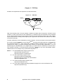
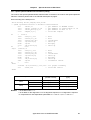
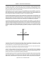
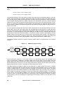
Chapter 2 FIR Filter
FIR filters are implemented as depicted in the flowchart below.
Figure 2-1:
data in
FIR-Filter
T
M1
T
M2
T
Mn-1
Mn
Σ
filtered data out
With each sampling clock, the input sample is shifted one stage further through the cascade of shift
registers (T). Each of the values is then multiplied by a coefficient (Mn) and all results are accumulated
(Σ). The accumulated result must be properly scaled to become the filtered output value. With suitably
scaled coefficients, the scaling of the output is just a right shift of the data and it is therefore not drawn
in the above flowchart.
The filter coefficients can be calculated by various programs. There are freeware or time limited evaluation version programs available from the internetNote 1 and also web based programs, which calculate
the coefficients onlineNote 2. Also commercially available software packages can be usedNote 3. The
coefficients are usually presented as floating point numbers, so that the filter amplification is one. For
implementing the calculated filter on an integer CPU, one must scale the coefficients, so that the maximum possible resolution is achieved without generating overflows on any of the intermediate results.
Useful tools for such scaling are any spread sheet programsNote 4.
Notes: 1. For downloadable filter design programs visit:
http://www.filter-solutions.com/
http://www.systolix.co.uk/about.htm
2. For online filter design programs visit:
http://www.nauticom.net/www/jdtaft/
http://www-users.cs.york.ac.uk/~fisher/mkfilter/
http://www.digitalfilter.com/
3. For commercial filter design software visit:
http://www.mathworks.com/
4. For a free office package including spreadsheet program for Linux and Windows see:
http://www.openoffice.org/
8
Application Note U17285EE2V0AN00
Chapter 2
FIR Filter
2.1 Practical FIR Implementation
A straightforward implementation of an nth order FIR filter would shift the old samples up in a buffer,
store the new sample at the beginning of that buffer and then perform n multiply and accumulate operations. It turns out that this is almost the best possible strategy for a general purpose RISC processor like
the V850. More dedicated signal processing architectures like DSPs, have special means to efficiently
support ring buffers and they have multiply and accumulate units, which calculate such a result in one
clock cycle. Sometimes more than one such MAC units are implemented.
When designing software for a filter architecture, one has the choice of speed or space optimization,
but one can usually not have both at the same time. The different approaches are discussed below
while always considering the V850 and V850E pipeline structure. We have simulated the code with the
Green Hills V850 and V850E simulators and also tested it on real devices to verify the results as simulators are not always cycle accurate. If the results differ, we specify those from the real device. For the
V850E core we have used the V850E/ME2 and its on-chip timer for timing measurements. It has a limited resolution as it is clocked with 1/8th of the CPU frequency. Therefore the clock speeds are accurate
to those eight clocks. A V850/SB1 emulator with built-in clock timer has been used for V850 timing
measurements. Therefore these timings are accurate to the clock.
Code and data were located into on-chip instruction and data memories, so that the system can take
advantage of the internal Harvard architecture and of the one-clock access times. The performance will
degrade significantly, if any of these memories is chip external. Minor performance degradation might
be observed when the program is executed from on-chip flash memory with interleaved access.
The filter order n for practical FIR filters is usually between 16 and 128, with possible exceptions at both
ends. We have more or less arbitrarily selected a 48th order FIR filter, but the measurement results can
be easily re-calculated for the actual filter order.
To test the filters, they can be applied to real signals stored in a standard wave file. Such signals can be
real life signals recorded through a sound-card or synthetically generated signals. A useful program to
record, generate and analyze wave-files is CoolEdit (www.cooledit.com). In order to process an input
wave file and generate a filtered output wave file, the variable WAVEOUT must be defined. The path
names to the input and output files can be adapted in the source code (main.c) or otherwise the standard Green Hills path (<GHS>\MyProjects\) applies. The variable SIMULATE suppresses some code
generation, which is only useful on a real device (like starting and stopping timers for timing measurement). It is suggested to define that variable for simulation and it must be undefined for running on real
devices. Note that the software is not written as a push-button benchmark. Some tweaking is required
to enable the individual filter algorithm to be tested. An emulator is necessary for timing measurements.
We have defined a FILTER structure, which describes the FIR- or Hilbert-filter. The C-code type definition is as follows:
typedef struct {
WORD size;
WORD scale;
SSHORT *coeff;
SSHORT *data;
} FILTER;
Application Note U17285EE2V0AN00
9
Chapter 2
FIR Filter
In assembler files, we use the following code to reference the members of a FILTER:
filter_size
filter_scale
filter_coeff
filter_data
.equ
.equ
.equ
.equ
0
4
8
12
-----
offset
offset
offset
offset
to
to
to
to
number of coefficients (WORD)
scale
coefficient pointer
data pointer
All add instructions for FIR-filters and Hilbert-transformations are standard add instructions, not saturated adds. That is because these filter types are inherently stable and overflows will not occur if the
coefficients are properly scaled. IIR filters can be unstable and generate overflows. Therefore they use
the satadd instructions to accumulate the individual results.
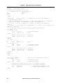
2.1.1 Size optimized FIR (firsz)
The size optimized version implements a software loop, which loops n times through the mac-code.
Especially for a RISC architecture like the V850, that strategy imposes an instruction time penalty of
one clock for the compare with n instruction and one (V850E) or two (V850) clocks for the discarded
pipeline when the branch is taken (n-1 times). One also needs to implement a pointer to the sample and
another one to the coefficients, each of which must be incremented each time. On the other hand, this
code is rather compact and it is the best choice for non time critical applications. Here is a source code
listing of the assembler macro:
.macro firsz
filter,sample,size,scale
-- size optimized version
mov
filter,r7
-mov
size-1,r11
-ld.w
filter_coeff[r7],r8
-ld.w
filter_data[r7],r7
-addi
2*(size-2),r8,r8
-st.h
sample,0[r7]
-addi
2*(size-2),r7,r7
-ld.h
2[r8],r10
-ld.h
2[r7],r9
-ld.h
0[r7],r6
-mulh
r9,r10
-.align
4
get address of FILTER struct
get filter order - 1
get address of coefficients to r8
get address of data to r7
we start from the end
store new sample
we start from the end
coefficient
data
data
multiply
1:
ld.h
st.h
mulh
add
add
add
add
ld.h
bne
satsubi
sar
0[r8],r9
-r6,2[r7]
-r6,r9
--2,r7
--2,r8
-r9,r10
--1,r11
-0[r7],r6
-1b
--(1<<(scale-1)),r10,r10-scale,r10
--
coefficient
upshift
multiply
next data (go down)
next coefficient (go down)
accumulate result
loop counter
data
branch back while not finished
for proper rounding
scale the result
.endm
10
Application Note U17285EE2V0AN00
Chapter 2
FIR Filter
The loop has been optimized to (hopefully) the maximum possible degree. On first sight one might be
surprised about the order of the instructions, but they have been arranged in such a way, that the
instruction pipeline does not stall unnecessarily. No instruction refers to data, which was produced by
the previous instruction (even though we could have done that in most cases, because of the built-in
pipeline short path). That is the reason, why even the conditional branch at the end is preceded by an
instruction that does not seem to belong there. The condition code for that branch was set by the add
instruction two lines earlier and it is unaffected by the preceding load.
If the beginning of the loop were not aligned to a word boundary, then the CPU would need two clocks
instead of one to load that instruction after a branch takes place. Therefore an align pseudo instruction
has been inserted, which will generate a nop if that is required to achieve the alignment. That nop
instruction costs one clock but saves n-1 clocks for the loop.
The last two instructions in the macro above scale the result back to a 16-bit signed integer. The sar
instruction divides the 32-bit wide intermediate result by 2scale and discards the low order bits, i.e. the
remainder. This is effectively a truncation of the 32-bit integer to a 16-bit integer. As the truncated part
may have any value between 0 and 1, the signal level is effectively shifted by ½ bit towards the negative
minimum. That may not be significant for an FIR filter, but it becomes important for the cascaded IIR filters, which are discussed later in this document. The error sums up and gradually adds a negative DC
offset to the signal. Therefore the satsubi instruction is used to add that ½ bit to compensate this DC
offset. satsubi is used with a negative adder, because there is no sataddi instruction on the V850 or
V850E devices. A side effect of this compensation is the reduced noise floor of the output signal,
because it rounds the result up or down instead of just truncating it. The signal to noise ratio is thus
improved by 3 dB (since 1 bit of resolution impacts the noise by 6 dB).
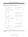
2.1.2 Speed optimized FIR (firsp)
The speed optimized version simply issues the same code once per filter order. As we can see below,
one can occupy the pipeline very efficiently with that strategy, but at the expense of code space. Fortunately we can save a few instructions per iteration compared with the space optimization, because the
offsets to data and coefficients are hard coded and therefore the pointer registers need not be updated.
Also the loop counter and the conditional branch are avoided. That reduces the number of instructions
per iteration to just four or five instead of nine in the size optimized version. By arranging the instructions in the optimum sequence, one can achieve an instruction pipelining without any stalls, i.e. one
instruction is executed per clock cycle.
Here is the optimized code for one mac-cycle:
ld.h
add
ld.h
st.h
mulh
2*nr[r7],r6
r9,r10
2*nr[r8],r9
r6,2*(nr+1)[r7]
r6,r9
-- data
-- accumulate result
-- coefficient
-- upshift
-- multiply
As explained above, this code sequence is cascaded n times for speed optimization. The fourth instruction (st.h) is even omitted in the first block, because that buffer value is discarded. nr is counted down
from the filter order n-1 to zero and so the offsets to r7 and r8 are hard coded without the need to
update any of these two registers, which have to be initialized with pointers to the data buffer and the
coefficients.
None of the instructions refers to data, which is only calculated in the preceding instruction. Therefore a
cascade of n blocks takes n*5 clocks to execute. An exception to this statement is the code for the first
stage, which was moved out of the loop, because it is a bit special.
Application Note U17285EE2V0AN00
11
Chapter 2
FIR Filter
The code has been implemented in macros, so that it can be automatically replicated for the filter order
n. macsd is the inner part of the fir filter, which replicates the code <size-1> times and omits the accumulation for the first loop, because the multiplication result is already stored in the accumulator register.
That avoids additional instructions to clear this register.
.macro macsd
size
-nr
=
size-1
ld.h
2*nr[r7],r6
-ld.h
2*nr[r8],r10
-mulh
r6,r10
-.rept
size-1
nr
=
nr-1
ld.h
2*nr[r7],r6
-.if (nr <(size-2))
add
r9,r10
-.endif
ld.h
2*nr[r8],r9
-st.h
r6,2*(nr+1)[r7]-mulh
r6,r9
-.endr
.endm
mac and shift data
data
coefficient
multiply
data
accumulate result
coefficient
upshift
multiply
firsp is the outer part of the filter and it is the only macro that is called by the user. fir implements the initialization of the registers, the accumulation of the results from the final multiplication and the scaling of
the result.
.macro firsp
filter,sample,size,scale
-- speed optimized version
mov
filter,r7
-ld.w
filter_coeff[r7],r8
-ld.w
filter_data[r7],r7
-st.h
sample,0[r7]
-macsd
add
satsubi
sar
get address of FILTER struct
get address of coefficients to r8
get address of data to r7
store new sample
size
r9,r10
-- accumulate result from last mult.
-(1<<(scale-1)),r10,r10 -- for proper rounding
scale,r10
-- scale the result
.endm
2.1.3 Improved speed optimized FIR (firisp)
The previously described speed optimized FIR version can even be improved by another 20% (4 clocks
per filter order instead of 5 clocks). That improvement is achieved through hard coding the coefficients
into the instructions, i.e. taking mulhi instead of the mulh instruction. Using the coefficient as immediate
operand saves the load instruction and hence one clock cycle. It might be a disadvantage in some
applications, that the coefficients are no longer stored in the data memory. That prevents the dynamic
update of coefficients in the case of adaptive filters. Therefore we have analysed both kinds of speed
optimized versions.
Also coding that version of a speed optimized filter is a little bit annoying because macro handling with
the Green Hills macro assembler has its limitations. It does not support a variable number of parameters and therefore one cannot write a single macro for all filter orders. Therefore we have coded three
different types of macros. firisp_init must be called first to initialize the subsequent macros. Its only
parameter is the order of the filter. Any combination of firisp or firisp_n macros is used to issue the
12
Application Note U17285EE2V0AN00
Chapter 2
FIR Filter
instructions for the individual filter stage and finally firisp_end must be called to accumulate the final
product and scale the result. A sample sequence of macro calls for a 48th order filter is shown below:
mov
ld.w
_etp,r7
-- get address of FILTER struct
filter_data[r7],r7 -- get address of data to r7
firisp_init
firisp
firisp
firisp
firisp
firisp
firisp
firisp
firisp
firisp_2
firisp_2
firisp_2
firisp_2
firisp_4
firisp_4
firisp_8
firisp_16
firisp_end
etp_size
16
-102
-223
-324
-307
-128
147
352
321, 21
-379, -584
-370, 215
805, 919
296, -821, -1705, -1500
252, 3233, 6391, 8416
8416, 6391, 3233, 252, -1500, -1705, -821, 296
919, 805, 215, -370, -584,-379, 21, 321,352, 147,
-128, -307, -324, -223, -102, 16
etp_scale
firisp, firisp_2, firisp_4, firisp_8 and firisp_16 can be combined arbitrarily. The above sequence is just for
demonstration and it is identical to:
mov
ld.w
firisp_init
firisp_8
firisp_8
firisp_8
firisp_8
firisp_8
firisp_8
firisp_end
_etp,r7
-- get address of FILTER struct
filter_data[r7],r7 -- get address of data to r7
etp_size
16, -102, -223, -324, -307, -128, 147, 352
321, 21, -379, -584, -370, 215, 805, 919
296, -821, -1705, -1500, 252, 3233, 6391, 8416
8416, 6391, 3233, 252, -1500, -1705, -821, 296
919, 805, 215, -370, -584,-379, 21, 321
352, 147, -128, -307, -324, -223, -102, 16
etp_scale
This sequence expects the input sample to be passed in r6 and it returns the result in r10 according to
the Green Hills calling convention. Note that this code starts processing again from the end of the
buffer. Therefore the coefficients must be specified in reverse order, which is normally no difference as
they are symmetric.
Each firisp macro is resolved to the following code:
ld.h
add
st.h
mulhi
2*nr[r7],r6
-r9,r10
-r6,2*(nr+1)[r7]-coeff,r6,r9
--
data
accumulate result
upshift
multiply
As an exception, the first macro uses r10 for the multiplication result and the second one omits the add
instruction.
Application Note U17285EE2V0AN00
13
Chapter 2
FIR Filter
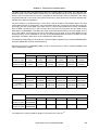
The following table lists the execution times and the code sizes of the previously described FIR filter
implementations:
Speed
[number of clocks]
Code size
[byte]
V850 core
11*n+k+1
72+2*k+2*m
V850E core
10*n+k+1
70+2*k+2*m
V850 core
5*n+12
16*n+18
V850E core
5*n+8
16*n+16
V850 core
4*n+9
14*n+18
V850E core
4*n+9
14*n+16
implementation
firsz
firsp
firisp
Remark:
n is the filter order. n > 1.
k is an adder for the alignment: k=0 if no alignment required, k=1 if alignment is required
m compensates for size dependent optimization: if n < 17: m = 0; if n >= 17: m = 1
The data sizes are not specified in the above table. One halfword per filter order is required to store the
samples and another halfword for the coefficients. The FILTER structure is 16 bytes long and it is
required once per filter. The improved speed optimized implementation requires only the storage for the
samples.
Finally we should explain why we have not used one of the most obvious optimization techniques, taking advantage of the symmetry of the coefficients. FIR filter coefficients are usually symmetric to their
center, i.e. c[0]=c[n-1], c[1]=c[n-2] and so on. Therefore one can first add the data and then multiply it
with the coefficient ((d[0]+d[n-1])*c[0], (d[1]+d[n-2])*c[1], …). That saves half of the multiplications and
half of the coefficient space.
There are two problems, however, with this algorithm, overflows and ring buffer handling. With 16-bit
data we might generate an overflow as the result of the addition is 17-bits wide, but the subsequent
multiplication is 16-bit*16-bit. One could scale the input data to 15-bit but that decreases its signal to
noise ratio by 6dB. Difficult ring buffer handling seems to be the major drawback of this symmetry optimization. While filtering, we move the data upward through the buffer, which works well, because the
previous data may be overwritten. That is not true, if we start from both ends of the buffer. We could
move up only the upper half and when finished move only the remaining data upward. Such a loop cannot be optimized very well, because the pipeline will often stall while waiting for the data. The advantage of such an algorithm seems to be negligible also due to the fact, that a multiplication on the V850/
V850E takes only one clock cycle.
14
Application Note U17285EE2V0AN00
Chapter 3 Special Versions of FIR Filters
3.1 Interpolation Filter
Interpolation filters are required when the sampling frequency of a signal is increased, i.e. the signal is
up-sampled. Up-sampling is generally achieved by inserting samples with the value zero between the
original sample. For two-times up-sampling, one would insert zero between every other original sample.
Doing so, one gets twice as many samples, as originally. The frequency spectrum, however, contains
the original frequency, but also its alias frequencies left and right of the original sampling frequency.
When up-sampling an original 3 kHz signal sampled by 16 kHz to 32 kHz by this method, on gets frequency components at 3 kHz, 13 kHz, 19 kHz and 29 kHz.
The unwanted frequencies above 3 kHz can be easily filtered by a low pass FIR filter as described
above. The effect of that low pass filter in the time domain is an interpolation of the original samples.
Therefore this kind of filter is called an interpolation filter.
For the specific purpose of interpolation, the FIR filter can be significantly optimized, because every
second sample is zero and therefore the respective multiplication result is also zero. We have redesigned the FIR filter macro to take that into account.
Interpolation filters are usually of relatively low order (4~16) and the filter parameters are fixed, i.e.
adaptive filters are not required. Therefore we have only implemented the improved speed version with
coefficients encoded as immediate values. In theory, up-sampling is possible by any integral multiple.
The practical limitation is the size of the interpolation filter, however. The filter must at least cover two
original samples and therefore the filter size increases with increasing up-sampling ratio. The example
below is made for a ratio of two. Other ratios could be easily derived. The filter order must be even.
Application Note U17285EE2V0AN00
15
Chapter 3
Special Versions of FIR Filters
.macro
ipf2_init size
-- initialize interpolation filter
-- *** FIRST macro for initialization ***
nr
=
(size/2)-1
order
=
size
init
=
1
.endm
.macro ipf2
coeff2,coeff1
-- issued once per two coefficients
-- Interpolation filter
-- note that we start from the top, so the coefficients must be reversed
-- (which is normally no difference as they are symmetric)
-- if (init == 1): r6 = sample; r7 = *data, r8 and r9 are temporary
register
-- if (init!= 1): r10 and r11 = accumulator; r7 = *data, r6, r8 and r9 are
temporary registers
-- r10 and r11 return first and second interpolated samples
.if (init == 1)
.if (order != 2)
st.h
r6,0[r7]
-- store new sample
ld.h
2*nr[r7],r6
-- data
.endif
mulhi coeff1,r6,r10 -- multiply
mulhi coeff2,r6,r11 -- multiply
firstm =
1
.endif
.if (init != 1)
nr
=
nr-1
ld.h
2*nr[r7],r6
-- data
.if (firstm != 1)
add
r8,r10
-- accumulate result
add
r9,r11
-- accumulate result
.endif
st.h
r6,2*(nr+1)[r7]-- upshift
mulhi coeff1,r6,r8
-- multiply
mulhi coeff2,r6,r9
-- multiply
firstm =
0
.endif
init
=
0
.endm
.macro ipf2_endscale
-- wrap up for interpolation filter
.if (order != 2)
add
r8,r10
-- accumulate result
add
r9,r11
-- accumulate result
.endif
satsubi-(1<<(scale-1)),r10,r10-- for proper rounding
satsubi-(1<<(scale-1)),r11,r11-- for proper rounding
sar
scale,r10
-- return first sample in r10
sar
scale,r11
-- return second sample in r11
.endm
16
Application Note U17285EE2V0AN00
Chapter 3
Special Versions of FIR Filters
The interpolation filter takes one sample as input value in register r6 and it returns two samples in the
register pair r10 and r11. Multiple interpolation filters can be cascaded for higher up-sampling ratios.
As with the improved speed optimized version before, we have to issue three different macros for one
interpolation filter. Here is an example for up-sampling by eight:
-- 1st interpolation
ld.h
zdaoff(_s0i)[r0],r6
-- get filter input value
mov
_fi1,r7
-- get address of FILTER struct
ld.w
filter_data[r7],r7
-- get address of data to r7
ipf2_init 12
ipf2_10
-578, -1986, 68, 11061, 24131, 24131, 11061, 68, -1986, -578
ipf2_end 15
st.h
r10,zdaoff(_s1i)+0[r0]
st.h
r11,zdaoff(_s1i)+2[r0]
-- 2nd interpolation
mov
2,r14
mov
0,r13
mov
0,r15
-- loop counter for upsampling
-- source sample index
-- destination sample index
upsample2:
ld.h
zdaoff(_s1i)[r13],r6
mov
_fi2,r7
ld.w
filter_data[r7],r7
ipf2_init 8
ipf2_8 197, 2781, 10567, 19222,
ipf2_end 15
st.h
r10,zdaoff(_s2i)+0[r15]
st.h
r11,zdaoff(_s2i)+2[r15]
add
add
add
bnz
2,r13
4,r15
-1,r14
upsample2
-- 3rd interpolation
mov
4,r14
mov
0,r13
mov
0,r15
-- get filter input value
-- get address of FILTER struct
-- get address of data to r7
19222, 10567, 2781, 197
-- address next short element in array
-- loop counter for upsampling
-- source sample index
-- destination sample index
upsample3:
ld.h
zdaoff(_s2i)[r13],r6
-- get filter input value
mov
_fi3,r7
-- get address of FILTER struct
ld.w
filter_data[r7],r7
-- get address of data to r7
ipf2_init 8
ipf2_8 -950, -691, 9400, 25008, 25008, 9400, -691, -950
ipf2_end 15
st.h
r10,zdaoff(_s3i)+0[r15]
st.h
r11,zdaoff(_s3i)+2[r15]
The ipf2 macro takes 2 coefficients. For better readability, we have defined macros ipf2_n, with
n={2,4,6,8,10,12,14,16}, that take more coefficients. The intermediate values are stored in the arrays
s1i, s2i and s3i.
Application Note U17285EE2V0AN00
17
Chapter 3
Special Versions of FIR Filters
The following table lists the execution times and the sizes of the previously described interpolation filter:
Speed
[number of clocks]
Size
[byte]
V850 core
n=2: 6
n>2: 6*n/2+4
n=2: 20
n>2: 20*n/2+8
V850E core
n=2: 6
n>2: 6*n/2+4
n=2: 20
n>2: 20*n/2+8
implementation
ipf2
Remark:
n is the filter order.
n must be an even number and higher than 1.
3.2 Averaging filter
A very simple version of an FIR filter is a filter of 2nd order where both coefficients are 0.5. Each sample
is divided by 2 and the result is accumulated, which is nothing else than the average of both samples.
Therefore this filter is often called an averaging filter. Very low frequencies (compared to the sampling
frequency) pass this filter very well, because subsequent samples are not much different anyway. The
frequency fs/2 is totally suppressed, because subsequent samples have opposite values and cancel
out. Frequencies in the vicinity of fs/2 are still attenuated to a degree that depends on their offset from
fs/2.
The averaging filter is useful as an interpolation filter for higher frequencies, at which the aliases of the
signal frequency come very close to fs/2. Averaging filters are especially simple to implement in
FPGAs, because a multiplier is not needed. The filter just adds two samples and shifts the result right
by one bit.
For the purpose of up-sampling by two, two averaging filters can be cascaded very easily. As described
above, every other sample is zero and therefore the first averaging filter just duplicates the original samples. That is no computation task at all and it is performed implicitly. The second averaging filter calculates the average values for subsequent samples. Implementing an averaging filter for interpolation in
software for the V850 is very simple, as this macro demonstrates:
.macro ipfa
data,old
-- Averaging interpolation filter
-- data = sample, old = pointer to old sample
-- r10 and r11 return first and second interpolated samples
ld.h
0[old],r10
-- get previous sample
st.h
data,0[old]
-- save current sample
add
data,r10
-- sum old and current
sar
1,r10
-- generate average
mov
data,r11
-- second sample is original sample
.endm
This macro gets one sample and generates two samples, the first one in r10 and the second one in r11.
Therefore it up-samples by two and low pass filters the output.
18
Application Note U17285EE2V0AN00
Chapter 3
Speed
[number of clocks]
Size
[byte]
V850 core
5
14
V850E core
5
14
implementation
ipfa
Special Versions of FIR Filters
3.3 Hilbert Transformation
A Hilbert transform is used for 90° phase shifting of an input signal. It is a special case of an FIR filter: it
has an odd number of coefficients and every second coefficient is zero. The coefficients are anti-symmetric, which means that a coefficient on the left side has a counterpart of equal magnitude but
reversed sign on the right side. One could use the above FIR programs to run a Hilbert transformation,
but the special properties call for some more sophisticated optimization techniques.
The most obvious is based on the fact that every second coefficient is zero. The respective multiplication and addition can therefore be skipped. The number of mac cycles is so reduced to (n-1)/2. Unfortunately all data samples need to be shifted in the ring buffer and not just those whose coefficient is zero.
Taking advantage of the anti-symmetry is again not possible for the same reasons as with the FIR filter.
Even though the data samples have to be subtracted and not added before multiplication, we may generate an over- or underflow and therefore we would need 17-bits.
Again we have implemented space and speed optimized versions, which are shown below.
Application Note U17285EE2V0AN00
19
Chapter 3
Special Versions of FIR Filters
3.3.1 Space optimized Hilbert transformation (hilbsz)
The code for the Hilbert transformation is based on the code for the FIR filter. Therefore please refer to
the FIR filter description at page 8.
Here is a listing of the hilbsz macro:
.macro hilbsz filter,sample,size,scale
-- size optimized version of Hilbert transformation
mov
filter,r7
-- get address of FILTER struct
mov
(size-3)/2,r12
-- get loop count
ld.w
filter_coeff[r7],r8
-- get address of coefficients to r8
ld.w
filter_data[r7],r7
-- get address of data to r7
addi
2*(size-5),r8,r8
-- we start from the end
st.h
sample,0[r7]
-- store new sample
addi
2*(size-5),r7,r7
-- we start from the end
ld.h
ld.h
ld.h
st.h
mulh
st.h
ld.h
.align
2*2+2[r8],r10
2*2+2[r7],r6
2*2[r7],r11
r6,2*2+4[r7]
r6,r10
r11,2*2+2[r7]
2[r7],r6
4
--------
ld.h
ld.h
st.h
mulh
st.h
add
add
add
add
ld.h
bne
satsubi
sar
0[r7],r11
-2[r8],r9
-r6,4[r7]
-r6,r9
-r11,2[r7]
--4,r7
--4,r8
-r9,r10
--1,r12
-2[r7],r6
-1b
--(1<<(scale-1)),r10,r10-scale,r10
--
coefficient
data
data
shift up
multiply
shift up
data
1:
data
coefficient
shift up
multiply
shift up
next data (go down)
next coefficient (go down)
accumulate result
loop counter
data
branch back while not finished
for proper rounding
scale the result
.endm
20
Application Note U17285EE2V0AN00
Chapter 3
Special Versions of FIR Filters
3.3.2 Speed optimized Hilbert transformation (hilbsp)
The code for the speed optimized Hilbert transformation is based on the code for the speed optimized
FIR filter. Therefore please refer to the FIR filter description at page 9.
Here is a listing of the hilbsp macro:
.macro hilbsp filter,sample,size,scale
-- speed optimized version of Hilbert transformation
mov
filter,r7
-- get address of FILTER struct
ld.w
filter_coeff[r7],r8
-- get address of coefficients to r8
ld.w
filter_data[r7],r7
-- get address of data to r7
st.h
sample,0[r7]
-- store new sample
nr
nr
.rept
nr
.endr
=
size-3
ld.h
2*nr[r7],r11
ld.h
2*nr+2[r7],r6
ld.h
2*nr+2[r8],r10
st.h
r6,2*nr+4[r7]
mulh
r6,r10
st.h
r11,2*nr+2[r7]
=
nr-2
(size-3)/2
ld.h
2*nr[r7],r11
ld.h
2*nr+2[r7],r6
ld.h
2*nr+2[r8],r9
st.h
r6,2*nr+4[r7]
mulh
r6,r9
st.h
r11,2*nr+2[r7]
add
r9,r10
=
nr-2
-------
data
data
coefficient
shift up
multiply
shift up
--------
data
data
coefficient
shift up
multiply
shift up
accumulate result
satsubi -(1<<(scale-1)),r10,r10-- for proper rounding
sar
scale,r10
-- scale the result
.endm
Speed
[number of clocks]
Size
[byte]
V850 core
13*(n-3)/2+16+k
92+2*k+2*m
V850E core
12*(n-3)/2+16+k
90+2*k+2*m
V850 core
7*(n-1)/2+10
24*(n-1)/2+22
V850E core
7*(n-1)/2+8
24*(n-1)/2+20
implementation
hilbsz
hilbsp
Remark:
n is the filter order. n > 1.
k is an adder for the alignment: k=0 if no alignment required, k=1 if alignment is required
m compensates for size dependent optimization: if n < 35: m = 0; if n >= 35: m = 1
Application Note U17285EE2V0AN00
21
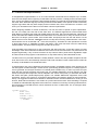
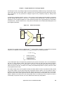
Chapter 4
IIR Filter
IIR filters are implemented in their direct form 2 as depicted belowNote.
Figure 4-1:
data in
k
Σ
IIR Filter
b0
Σ
filtered data out
T
a1
b1
T
a2
b2
Note: We have selected to implement the direct form 2 instead of direct form 1, because it requires
less storage elements and therefore it makes buffer handling much simpler. It reduces the number of memory read/write operations as well as the required memory size.
The above structure is a 2nd order IIR filter. By choosing zero for a2 and b2, the filter reduces to a 1st
order IIR filter. IIR filters of higher order are usually implemented by cascading such 1st and 2nd order
IIR blocks. Higher order blocks are still possible, but they become unpractical to design and to implement so that they are stable. To keep things simple, we have implemented and benchmarked code for
the above building blocks. The macros can be easily cascaded for higher order filters. The execution
times and code sizes can simply be added.
As an IIR filter block is rather small compared to a lengthy FIR filter, it is not useful to implement it in a
space optimized structure. Therefore we have only generated one version each for the 1st order and for
the 2nd order block, which are speed optimized and which do not contain any branches.
Intermediate results in an IIR filter chain have to be truncated to avoid overflows. In order to compensate for DC offsets, the values are properly rounded before being truncated.
22
Application Note U17285EE2V0AN00
Chapter 4
IIR Filter
Two similar macros have been written for IIR filters, one for a first order block (iir1) and another one for
a second order block (iir2). They both take the filter coefficients as immediate arguments. Here are the
listings of these two macros:
.macro iir1
sample,data,scale,k,b1,b0,a1
-- 1st order IIR filter block
-- do not use r6, r7, r8 or r10 for data pointer
-- do not use r8 for input sample
-- output sample is returned in r10
ld.h
0[data],r8
mulhi
k,sample,r10
-- sample * k
mulhi
-a1,r8,r6
mulhi
b1,r8,r7
satadd
r6,r10
satsubi
-(1<<(scale-1)),r10,r10
-- for proper rounding
sar
scale,r10
st.h
r10,0[data]
mulhi
b0,r10,r10
-- pipeline stall
satadd
r7,r10
satsubi
-(1<<(scale-1)),r10,r10
-- for proper rounding
sar
scale,r10
-- return result in r10
.endm
.macro iir2
sample,data,scale,k,b2,b1,b0,a2,a1
-- 2nd order IIR filter block
-- do not use r6, r7, r8, r9, r10 for data pointer
-- output sample is returned in r10
mulhi
k,sample,r10
-- sample * k
ld.h
2[data],r7
ld.h
0[data],r8
mulhi
-a2,r7,r9
mulhi
-a1,r8,r6
satadd
r9,r10
st.h
r8,2[data]
satadd
r6,r10
mulhi
b2,r7,r6
satsubi
-(1<<(scale-1)),r10,r10
-- for proper rounding
sar
scale,r10
mulhi
b1,r8,r9
st.h
r10,0[data]
mulhi
b0,r10,r10
satadd
r6,r9
satadd
r9,r10
satsubi
-(1<<(scale-1)),r10,r10
-- for proper rounding
sar
scale,r10
-- return result in r10
.endm
Application Note U17285EE2V0AN00
23
Chapter 4
IIR Filter
The IIR macros can be optimized almost to the same degree as the FIR macros. There is only one
pipeline stall in the iir1 macro. Here are the benchmark results for the IIR filter blocks:
Speed
[number of clocks]
Size
[byte]
V850 core
13
40
V850E core
13
40
V850 core
18
60
V850E core
18
60
implementation
iir1
iir2
One additional instruction is required for each filter block to setup a pointer to the sample memory. It is
not included in the above figures, so for cascading IIR filter blocks, it is necessary to add 1~2 clocks and
4~8 bytes per cascade. A sample cascade of two IIR filter blocks is shown below:
mov
iir1
mov
iir2
iir_data_1a,r11
-- get address of data area
r6,r11,15,4251,16384,16384,-28516
iir_data_2a,r11
-- get address of data area
r10,r11,14,2009,23277,-26861,23277,14629,-28597
The mov instruction is resolved to a native instruction on the V850E core, while a movhi and a movea
instruction is issued in case of a V850 core.
24
Application Note U17285EE2V0AN00
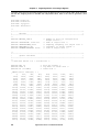
Chapter 5
Digital Synthesis of Analogue Signals
According to Fourier, any analogue signal can be synthesized by additive mixing of its spectral components, which are sine and cosine waves. Therefore, if we can generate sine and cosine waves of arbitrary frequencies, we can generate an analogue signal of any complexity simply by adding these
components.
A simple way to digitally generate a sine or cosine signal, is direct digital synthesis (DDS). That means
that we calculate the function y = sin(ωt) or y = cos(ωt) for every discrete time t. As both functions are
repetitive for every integral multiple of 2π, the function arguments can be generated by an accumulator
of finite bit size ρ, which overflows at 2π. This phase accumulator is the fundamental building block of a
direct digital synthesizer:
Figure 5-1:
Phase Accumulator
ρ
ρ
Phase
Register
Phase
Adder
Frequency
Register
f CLK
ρ
The frequency register must be initialized with the proper phase increment ϕ to generate the required
frequency f. It depends on the sampling clock fCLK according to the following equation:
ϕ = (2ρ * f) / fCLK
ϕ:
ρ:
f:
fCLK:
phase increment
accumulator bit size
output frequency
sampling frequency
In the subsequent step, the arguments generated by the phase accumulator, have to be translated to
the sine or cosine function values. This could be done by using the sin() and cos() library functions,
which are provided from the C runtime library. They return very precise float values, but they take a
rather long time to execute. Therefore one usually uses ROM lookup tables to quickly return the result
of the trigonometric function.
Two rather simple tricks can be applied to keep the lookup table as small as possible and still provide
very precise results. As sine and cosine have symmetric function values, one only needs to store a
quarter of a full wave and derive the other three quarters from this one. The second trick is to interpolate the function values if the argument does not exactly match with the lookup table entry. Linear interpolation between two entries from the lookup table does an excellent job. Even though the result is
occasionally not precise to the bit, it is much better than without any interpolation.
Application Note U17285EE2V0AN00
25
Chapter 5
Digital Synthesis of Analogue Signals
The high order bits from the phase register serve as address input for the lookup table, while the lower
bits are the weighing factor to calculate the interpolated value. Here is the code to generate a sine
wave:
#include
#include
#include
#include
<stdio.h>
<stdlib.h>
´mytype.h´
´Wavelib.h´
/*
+-----------------------------------------------------------------------+
|
Defines
|
+-----------------------------------------------------------------------+
*/
#define WEIGHT_SIZE 8
/* number of bits for interpolation
weight factor */
#define OUTPUTFILE ´sine.wav´
/* name of output file */
#define SAMPLINGFREQ 8000
/* sampling frequency for output file */
#define FREQUENCY 1333
/* frequency of output signal */
#define NUMBEROFSAMPLES 20000
/* size of output file */
/*
+-----------------------------------------------------------------------+
|
global variables
|
+-----------------------------------------------------------------------+
*/
/* ROM Sine Table: 1/4 = 256 entries */
#define BPS 16
#define LDTS 8
#define TS (1<<LDTS)
/* bits per sample */
/* log duals of table size */
/* table size */
_SWORD static table[TS] = {
0,
201,
402,
603,
1608,
1809,
2009,
2210,
3212,
3412,
3612,
3811,
4808,
5007,
5205,
5404,
6393,
6590,
6786,
6983,
7962,
8157,
8351,
8545,
9512,
9704,
9896, 10087,
11039, 11228, 11417, 11605,
12539, 12725, 12910, 13094,
14010, 14191, 14372, 14553,
15446, 15623, 15800, 15976,
16846, 17018, 17189, 17360,
18204, 18371, 18537, 18703,
19519, 19680, 19841, 20000,
20787, 20942, 21096, 21250,
22005, 22154, 22301, 22448,
23170, 23311, 23452, 23592,
24279, 24413, 24547, 24680,
25329, 25456, 25582, 25708,
26319, 26438, 26556, 26674,
27245, 27356, 27466, 27575,
28105, 28208, 28310, 28411,
28898, 28992, 29085, 29177,
29621, 29706, 29791, 29874,
30273, 30349, 30424, 30498,
26
804,
2410,
4011,
5602,
7179,
8739,
10278,
11793,
13279,
14732,
16151,
17530,
18868,
20159,
21403,
22594,
23731,
24811,
25832,
26790,
27683,
28510,
29268,
29956,
30571,
1005,
2611,
4210,
5800,
7375,
8933,
10469,
11980,
13462,
14912,
16325,
17700,
19032,
20317,
21554,
22739,
23870,
24942,
25955,
26905,
27790,
28609,
29358,
30037,
30643,
1206,
2811,
4410,
5998,
7571,
9126,
10659,
12167,
13645,
15090,
16499,
17869,
19195,
20475,
21705,
22884,
24007,
25072,
26077,
27019,
27896,
28706,
29447,
30117,
30714,
Application Note U17285EE2V0AN00
1407,
3012,
4609,
6195,
7767,
9319,
10849,
12353,
13828,
15269,
16673,
18037,
19357,
20631,
21856,
23027,
24143,
25201,
26198,
27133,
28001,
28803,
29534,
30195,
30783,
Chapter 5
30852,
31356,
31785,
32137,
32412,
32609,
32728,
30919,
31414,
31833,
32176,
32441,
32628,
32737,
30985,
31470,
31880,
32213,
32469,
32646,
32745,
Digital Synthesis of Analogue Signals
31050,
31526,
31926,
32250,
32495,
32663,
32752,
} ;
31113,
31580,
31971,
32285,
32521,
32678,
32757,
31176,
31633,
32014,
32318,
32545,
32692,
32761,
31237,
31685,
32057,
32351,
32567,
32705,
32765,
31297,
31736,
32098,
32382,
32589,
32717,
32766
/*
+-----------------------------------------------------------------------+
|
Function prototypes
|
+-----------------------------------------------------------------------+
*/
int main(int argc, char **argv, char **envp) ;
_SWORD get_amplitude(_LONG *phase, _LONG freq) ;
_SWORD get_from_table(_WORD index) ;
/*
+-----------------------------------------------------------------------+
|
int main(int argc, char **argv, char **envp)
|
+-----------------------------------------------------------------------+
|
|
| Main program
|
|
|
+-----------------------------------------------------------------------+
*/
int main(int argc, char **argv, char **envp)
{
WFILE *outputfile ;
/* output file */
_SLONG sample ;
_WORD i, index ;
_LONG phase ;
/* phase */
_LONG phi ;
/* phase increment */
outputfile = wfcreate((char *) OUTPUTFILE, 16, 1, (_LONG) SAMPLINGFREQ) ;
if (outputfile != NULL)
{
index = 0 ;
phase = 0 ;
phi = ((long long) FREQUENCY * (long long) 0x100000000) / SAMPLINGFREQ ;
for (i=0; i<NUMBEROFSAMPLES; i++)
{
sample = get_amplitude(&phase, phi) ;
wfputsample(&sample, outputfile) ;
}
wfclose(outputfile) ;
}
return(0);
}
Application Note U17285EE2V0AN00
27
Chapter 5
Digital Synthesis of Analogue Signals
/*
+-----------------------------------------------------------------------+
|
_SWORD get_amplitude(_LONG *phase, _LONG freq)
|
+-----------------------------------------------------------------------+
|
|
| Return amplitude for current phase and update phase.
|
|
|
+-----------------------------------------------------------------------+
*/
_SWORD get_amplitude(_LONG *phase, _LONG freq)
{
_WORD index ;
_SWORD val, val1, val2 ;
_LONG weight ;
index = (_WORD) (*phase >> (32 - (LDTS + 2))) ; /* +2 because of quarter
sine table */
val1 = get_from_table(index) ;
val2 = get_from_table(index+1) ;
weight = *phase >> (32 - (LDTS + 2 + WEIGHT_SIZE)) ;
weight = weight & ((1<<WEIGHT_SIZE) - 1) ;
val = val1 + (_SWORD) (((val2 - val1) * (_SLONG) weight)
/ (_SLONG) (1l<<WEIGHT_SIZE)) ;
*phase = *phase + freq ;
return(val) ;
}
/*
+-----------------------------------------------------------------------+
|
_SWORD get_from_table(_WORD index)
|
+-----------------------------------------------------------------------+
|
|
| Return amplitude for current index.
|
|
|
+-----------------------------------------------------------------------+
*/
_SWORD get_from_table(_WORD index)
{
_WORD quarter ;
_SWORD val ;
index = index & ((1<<(LDTS+2)) - 1) ;
quarter = index >> LDTS ;
index = index & ((1<<LDTS) - 1) ;
switch (quarter)
{
case 0: /* first quarter; take value as is */
val = table[index] ;
break ;
case 1: /* second quarter; take max or table[TS-index] */
if (index == 0)
val = (1<<(BPS-1)) - 1 ; /* max positive value */
else
val = table[TS-index] ;
break ;
case 2: /* third quarter; take value and make negative */
val = -table[index] ;
28
Application Note U17285EE2V0AN00
Chapter 5
Digital Synthesis of Analogue Signals
break ;
case 3: /* fourth quarter; as second, but negative */
if (index == 0)
val = -((1<<(BPS-1)) - 1) ; /* max positive value */
else
val = -table[TS-index] ;
break ;
}
return(val) ;
}
We use a set of functions to generate a wave file (wfcreate, wfputsample, wfclose), which can then be
analyzed with a suitable program. As described earlier, we have used CoolEdit (www.cooledit.com) for
this task.
For convenience on a 32-bit architecture we use a phase accumulator of 32-bit size. For a sampling
rate of 44.1 kHz, we can thus get a resolution of about 10 µHz, which seems like overkill, because a
phase accumulator of 16-bit would already give us a resolution of less than 1 Hz. On the other hand, a
16-bit accumulator would not have any advantage other than saving two bytes for the phase and two
bytes for the increment.
get_amplitude() is a function that calculates the amplitude for the current phase and updates the phase
value thereafter. get_amplitude() calls get_from_table twice to retrieve the two neighbour grid points
and then it performs the linear interpolation using the weighing factor from the lower bits of the phase
value.
An example for the DDS is found in the appendix, where this function is used to generate a DTMF signal.
Application Note U17285EE2V0AN00
29
Chapter 6 Fast Fourier Transform (FFT)
The FFT is a special implementation of the Discrete Fourier Transform. Both the DFT and the FFT are
used to determine the spectral components of a signal, i.e. they transform a signal from the time
domain into the frequency domain. The DFT is computationally costly, as it requires N2 complex multiplications and N*(N-1) complex additions. It also requires large memory tables to store N2 values for the
sine and cosine. N is the number of input samples and it is also the number of spectral lines at the output.
The effort to solve the DFT can be simplified, if ld(N) is an integer number, i.e. N = 2m. The total number
of complex multiplications is then reduced to N*m, which is much less than N2, especially for higher N.
N is usually in the order of 64 to 1024, but sometimes even much higher than that.
This application note will not cover the principles of the DFT or the FFT. There are many good
booksNote 1 on these topics and also a lot of internet resourcesNote 2. Here is a quote from “The Scientist and Engineer's Guide to Digital Signal Processing”: “While the FFT only requires a few dozen lines
of code, it is one of the most complicated algorithms in DSP. But don't despair! You can easily use published FFT routines without fully understanding the internal workings.” We have taken this remark seriously and have only implemented and tested the algorithm.
The FFT algorithm is subdivided into three blocks, the initialization of the sine and cosine tables, resorting of the input samples and execution of the fundamental butterfly operations. Optionally a windowing
function can be applied before the samples are reshuffled and often the complex output samples need
to be transformed into magnitude samples.
Here is the C-language source code for the FFT:
/*
+-----------------------------------------------------------------------+
|
Defines
|
+-----------------------------------------------------------------------+
*/
#define
LDORDER
10
/* ld(ORDER) */
#define
ORDER
(1<<LDORDER) /* order of FFT */
#define
PI
3.14159265359
#ifdef WINDOW
#define
WSCALE
#else
#define
WSCALE
#endif
8192.0
16384.0
/*
+-----------------------------------------------------------------------+
|
Function prototypes
|
+-----------------------------------------------------------------------+
*/
int main(int argc, char **argv, char **envp) ;
Notes: 1. For example: „Digitale Signalverarbeitung in der Nachrichtentechnik” from Peter Gerdsen
and Peter Kroeger, Springer Verlag, ISBN 3-540-61194-0
2. See http://www.dspguide.com/ for the book “The Scientist and Engineer's Guide to Digital
Signal Processing”
30
Application Note U17285EE2V0AN00
Chapter 6
Fast Fourier Transform (FFT)
/*
+-----------------------------------------------------------------------+
|
int main(int argc, char **argv, char **envp)
|
+-----------------------------------------------------------------------+
|
|
| Main program
|
|
|
+-----------------------------------------------------------------------+
*/
int main(int argc, char **argv, char **envp)
{
unsigned int i, j, k, m, r, ar, v ;
signed int z1, z2, z3, z4 ;
signed int xr, xi, yr, yi ;
signed int static fr[ORDER], fi[ORDER] ;
/* I&Q samples */
float static fm[ORDER] ;
/* magnitude samples */
signed int static zr[ORDER], zi[ORDER] ;
/* I&Q frequencies */
signed short static sint[ORDER], cost[ORDER] ; /* sine and cosine tables */
unsigned short static br[ORDER] ;
/* resorting table */
float frs, fis ;
#ifdef WINDOW
signed int ampl ;
#endif
/* initialize sin and cos tables */
for (i=0; i<ORDER; i++)
{
sint[i] = (signed short) (sin(i * 2 * PI / ORDER) * 32767) ;
cost[i] = (signed short) (cos(i * 2 * PI / ORDER) * 32767) ;
}
/* initialize resorting tables for bit-reversal */
for (i=0; i<ORDER; i++)
{
k = 0 ;
for (j=0; j<LDORDER; j++)
{
k |= (1&(i>>j))<<(LDORDER-j-1) ;
}
br[i] = (unsigned short) k ;
}
/* for testing, we generate the samples which we
for (i=0; i<ORDER; i++)
{
/* sample signal: frequency=6
amplitude=80%
frequency=19 amplitude=10%
frequency=35 amplitude= 7%
frequency=48 amplitude= 3%
zr[i] = ((signed int) ( 0.80 * cos(6.0 * i
+ (signed int) (-0.10 * sin(19.0 * i
+ (signed int) (-0.07 * cos(35.0 * i
+ (signed int) ( 0.03 * sin(48.0 * i
zi[i] = ((signed int) ( 0.80 * sin(6.0 * i
+ (signed int) ( 0.10 * cos(19.0 * i
+ (signed int) (-0.07 * sin(35.0 * i
+ (signed int) (-0.03 * cos(48.0 * i
will subsequently analyze */
phase shift
0°
phase shift 90°
phase shift 180°
phase shift 270°
* 2 * PI / ORDER)
* 2 * PI / ORDER)
* 2 * PI / ORDER)
* 2 * PI / ORDER)
* 2 * PI / ORDER)
* 2 * PI / ORDER)
* 2 * PI / ORDER)
* 2 * PI / ORDER)
Application Note U17285EE2V0AN00
*/
* 32767)
* 32767)
* 32767)
* 32767)) ;
* 32767)
* 32767)
* 32767)
* 32767)) ;
31
Chapter 6
Fast Fourier Transform (FFT)
}
#ifdef WINDOW
/* apply triangular window */
for (i=0; i<ORDER; i++)
{
if (i < ORDER/2)
ampl = i ;
else
ampl = ORDER - i - 1 ;
zr[i] = (2*zr[i]*ampl)/ORDER ;
zi[i] = (2*zi[i]*ampl)/ORDER ;
}
#endif
/* resort input samples */
for (i=0; i<ORDER; i++)
{
fr[i] = zr[br[i]] ;
fi[i] = zi[br[i]] ;
}
/* FFT butterfly operations */
for (m=1; m<=LDORDER; m++)
{
for (i=0; i<(1<<(LDORDER-m)); i++)
{
for (j=0; j<(1<<(m-1)); j++)
{
r = j + i * (1<<m) ;
ar = j * (ORDER>>m) ;
v = 1<<(m-1) ;
z1 = (cost[ar] * (fr[r+v]/(1<<(m-1))))/(1<<16-m)
z2 = (cost[ar] * (fi[r+v]/(1<<(m-1))))/(1<<16-m)
z3 = (sint[ar] * (fr[r+v]/(1<<(m-1))))/(1<<16-m)
z4 = (sint[ar] * (fi[r+v]/(1<<(m-1))))/(1<<16-m)
xr = fr[r] + z1 + z4 ;
xi = fi[r] - z3 + z2 ;
yr = fr[r] - z1 - z4 ;
yi = fi[r] + z3 - z2 ;
fr[r] = xr ;
fi[r] = xi ;
fr[r+v] = yr ;
fi[r+v] = yi ;
}
}
}
/* calculate the magnitudes and normalize to 1 */
for (i=0; i<ORDER; i++)
{
frs = (float) fr[i] * (float) fr[i] ;
fis = (float) fi[i] * (float) fi[i] ;
fm[i] = (sqrt(frs+fis)/ORDER) / WSCALE ;
}
return(0) ;
}
32
Application Note U17285EE2V0AN00
;
;
;
;
Chapter 6
Fast Fourier Transform (FFT)
The above code is based on sample Pascal code, which was published in „Digitale Signalverarbeitung
in der Nachrichtentechnik”. The code is surprisingly small, but nonetheless not straightforward to understand. In this chapter we will merely describe the functional blocks and refer the inclined reader to the
previously mentioned resources for further details.
ORDER defines the number of points for the FFT and LDORDER is the log2 of ORDER. A simple triangular windowing function is applied, if WINDOW is defined. Windowing changes the amplitude of the
input signal and therefore also the magnitude of the spectral component. This is fixed by defining a different scaling factor WSCALE, depending on whether or not windowing is applied.
The main program initializes the sine and cosine tables and the resorting table for the bit-reversal. The
sine and cosine tables are initialized by using the sin and cos functions of the C runtime library. That
makes the program rather flexible for testing purpose. In embedded systems one will usually implement
predefined tables to avoid the overhead of the trigonometric and floating point functions. Also the
resorting table may be generated at compile time, even though the advantage may be negligible.
The next block generates the waveform, which the subsequent code analyzes. In a real system, the
samples could come from the output of an I/Q mixer. Here one can play around with different frequency
components, different amplitudes and different phases. In this example we have taken a mixture of four
frequencies of different amplitude and phase shift. Make sure that none of the synthesized samples
exceeds the range of the signed halfword data type (-32768...32767). zr[ ] is the array for the real
(inphase, I) samples and zi[ ] holds the imaginary (quadrature, Q) samples as depicted in the image
below.
imaginary
Q=zi[ ]
ϕ
I=zr[ ]
real
The arrow moves counter-clockwise and its angular speed is the frequency of the signal, i.e. 2π/sec
(=360°/sec) is equal to 1 Hz. The phase of the signal is rather arbitrary, but it is commonly agreed, that
an arrow starting at I=1 and Q=0 has a phase shift of zero degrees.
The next block of code applies the optional triangular windowing function to the input data and subsequently resorts the input samples as required by the FFT algorithm.
The FFT butterfly operations finally transform the signal from the time domain into the frequency
domain. The complex nature of the input signal is preserved, i.e. the result of the FFT has maintained
the phase information. That is demonstrated in the sample code by using four different frequency components, each of which has a phase that is shifted by 90 degrees.
For optimum signal to noise ratio, it is important to keep the intermediate results as precise as possible,
while preventing overflows. The samples and the trigonometric tables are 16-bit signed halfword data
types and the intermediate results are stored in 32-bit signed words. Even though the trigonometric
tables store the function values in integer numbers between -32767 and 32767, these are really fracApplication Note U17285EE2V0AN00
33
Chapter 6
Fast Fourier Transform (FFT)
tions of 1/32767, as the real function values range from -1 to 1. Therefore the results of the multiplication with the trigonometric values have to be divided by 32767. Dividing through a power of two is most
easily done with a right shift operation, but unfortunately 32767 is not a power of two. We accept the
small error and divide through 32768, which is done by a 16-bit right shift operation. Even after 16 iterations for a 64k FFT, the accumulated error remains below 0.1% but we keep in mind that there is such
an error.
As the intermediate results quickly grow larger than halfwords, we have to scale them before the multiplication, so that the multiplication result always fits into a 32-bit word. This scaling is an art in itself.
Scaling too much will lose too many significant bits and decrease the signal to noise ratio, scaling too
little may generate overflows and so make the results unusable. The best approach would certainly be
to implement 64-bit arithmetic and entirely avoid scaling before multiplication. Sometimes it is possible
to check the numbers before the multiplication, at the expense of CPU time, and scale them just as
much as necessary. The simplest and fastest implementation scales the result as much as necessary
under worst case conditions. That is what we have done in the code that is shown above.
All multiplication results are effectively divided by 32768, but part of that division is done before the multiplication and the other part thereafter. It is probably difficult by analysis to find the rate at which the
intermediate results grow. Empirically we have found that they grow to less than double their value in
each iteration loop. Therefore we divide by 2m-1 before the multiplication and by 32768/2m-1 thereafter,
m being the outer loop counter. This empiric relation needs to be verified with real data.
The last part of the code does not strictly belong to the FFT algorithm anymore. It calculates the vector
length, i.e. the magnitude of the frequency component, from the I and Q samples.
6.1 FFT Benchmarks on V850
While it is possible to compile the above C-code for the V850, it is better to hand-optimize it. Therefore
we have implemented the algorithm also in assembly language. This way we have achieved a much
better execution time. The source code size of the assembler code is more than 300 lines and so it is
not included here. It can be found in the file “fft.850” within the zip-file that can be downloaded from the
NEC website along with this application note.
To measure the execution time, we have executed the code on a V850E/ME2 and on a V850E/ME3
device using internal code memory and internal or external data memory. The execution time includes
re-sorting the input data and executing the butterfly operations. It does not include the windowing function or the calculation of the magnitudes.
Due to the limited size of the internal data memory, we can only run FFTs up to an order of 512 with
internal memory. FFTs of larger order must use external memory. Therefore we have measured the
execution times for both configurations.
Benchmark results for V850E/ME2 (ME3) (data and code in internal memory):
FFT size
16
32
64
128
256
512
Assembler code
number of clocks
2608
(2456)
6216
(5808)
14464
(13464)
33032
(30688)
74320
(68968)
165208
(153200)
C code
number of clocks
9544
(9272)
23232
(23152)
55160
(54968)
128232
(125896)
296608
(290376)
662560
(648400)
34
Application Note U17285EE2V0AN00
Chapter 6
Fast Fourier Transform (FFT)
The ME3 code has been compiled with the E2-core compiler option. In all cases, the code was optimized for speed. As the table shows, the ME3 can only draw little advantage from its dual pipeline architecture. That is because much of the FFT algorithm is load and store and not arithmetic. Also many
instructions depend on the result of the previous instruction. Such sequences cannot be efficiently distributed to two instruction pipelines.
The FFT needs a lot of data memory. It must store I and Q samples, intermediate values, sine and
cosine tables and the re-sorting table. The intermediate values are of word type and the others are halfword type. The size of each table is the order of the FFT and so these tables alone require 18*ORDER
bytes of RAM. Therefore an FFT with an order above 512 will not fit anymore into the 16 kB on-chip
data RAM of a V850E/ME2. The /ME3 has a little more internal data memory and can handle an FFT
up to 1024 points. For larger FFTs it is then necessary to move some or all of these tables into the
external memory, which is SDRAM in the case of the V850E/ME2-ME3 test board. The ME3 can take
advantage of its built-in data cache, as the results below demonstrate.
The following results apply for all the above mentioned tables mapped into the external SDRAM (stack
and some global data is still in internal memory).
Benchmark results for V850E/ME2 (ME3) (code in internal memory, data in external SDRAM, data
cache enabled for the ME3):
FFT size
16
32
64
128
256
512
Assembler code
number of clocks
5104
(3912)
12112
(8960)
28232
(20472)
67288
(46368)
183408
(104184)
514960
(235040)
C code
number of clocks
10912
(9656)
26664
(23752)
63056
(56160)
148560
(128408)
390256
(295792)
957376
(668384)
FFT size
1024
2048
4096
8192
16384
32768
Assembler code
number of clocks
1193952
(561952)
2616448
(1748864)
5692160
(4480768)
12302848
(11254016)
26445312
(24237056)
56700928
(52024320)
C code
number of clocks
2226816
(1522976)
4611968
(3819520)
10027520
(8963328)
22039552
(19225088)
46044160
(40580096)
101529600
(87745536)
FFT size
65536
120502272
Assembler code
number of clocks (110745600)
226103296
C code
number of clocks (190650368)
The sample FFT code is limited by design to a maximum FFT size of 216.
Application Note U17285EE2V0AN00
35
Chapter 6
Fast Fourier Transform (FFT)
The V850E/ME2 can run at up to 150 MHz internal CPU speed. That means that a 256 point complex
FFT can be executed in less than 0.5ms (74320 clocks) and that a 64k complex FFT needs 0.8 s to
complete (120502272 clocks). A V850E/ME3 at 200 MHz can execute the 64k FFT in 0.56 s.
Note that the FFT code can be further optimized for the V850E2 core architecture. It supports a 32-bit
multiply-and-accumulate instruction with 64-bit intermediate results. We have not yet implemented
these optimizations. That is planned for a future revision of this application note.
36
Application Note U17285EE2V0AN00
Chapter 7 Application Examples
7.1 SSB Transmitter Audio Input Stage
As a practical example for the above described signal processing functions, we have implemented the
audio preprocessing for a single sideband (SSB) transmitter. SSB is a modulation technique, which is
still widespread in amateur radio transceivers. The basic idea of SSB is to transmit only one of the two
sidebands which are generated by an amplitude modulation of an RF signal. Also the residual carrier is
removed. The theory of generating an SSB signal is not very complicated, if trigonometric calculation
rules are understood. Here is a little bit of theory.
First of all we need to recall the relations for multiplication of trigonometric functions:
sin(α) * sin(β) = ½ cos(α-β) - ½ cos(α+β)
cos(α) * cos(β) = ½ cos(α-β) + ½ cos(α+β)
fa is the audio frequency (in today’s terms the payload), frf is the RF carrier frequency.
fa = sin(ωa*t)
frf = sin(ωrf*t)
We also need the 90° phase shifted versions of these signals, which are denoted with q:
faq = cos(ωa*t)
frfq = cos(ωrf*t)
Multiplying these two signals results in amplitude modulation (AM) of the carrier. If the audio frequency
signal is un-symmetric, i.e. always positive, then the result is the classical AM with carrier and two side
bands.
fmod = sin(ωrf*t) * (½ + ½ *sin(ωa*t))
fmod = ½ * sin(ωrf*t) + ¼ * cos((ωrf-ωa)*t) - ¼ * cos((ωrf+ωa)*t)
This AM signal consists of the carrier (1st term) and the sum and difference of the carrier and signal frequencies (2nd and 3rd terms). The carrier can be easily suppressed by a balanced modulation, in which
the audio signal is a signed signal and not always positive as above:
fmod = sin(ωrf*t) * sin(ωa*t)
fmod = ½ * cos((ωrf-ωa)*t) - ½ * cos((ωrf+ωa)*t)
This signed multiplication results in two sidebands without carrier.
If we do the same with the phase shifted quadrature signals, then we get:
fmodq = cos(ωrf*t) * cos(ωa*t)
fmodq = ½ * cos((ωrf-ωa)*t) + ½ * cos((ωrf+ωa)*t)
Application Note U17285EE2V0AN00
37
Chapter 7
Application Examples
Now it becomes obvious, how to generate only the upper (fmodusb) or lower (fmodlsb) sideband components:
fmodusb = fmodq - fmod = cos((ωrf+ωa)*t)
fmodlsb = fmodq + fmod = cos((ωrf-ωa)*t)
The sampling frequency of the RF signal is usually much higher than the sampling frequency of the AF
signal (in this case 4096 times higher). Modulating the RF signal directly with the AF signal will generate a virtually infinite number of alias frequencies. Therefore we must up-sample the audio input signal
to some higher sampling frequency, ideally to the same one that the RF signal uses. The RF sampling
frequency is in the order of 100 MHz and thus beyond the reach of a low cost software solution. Therefore it is a good idea to implement a hybrid system, which generates the computing intensive audio I
and Q signals by software and implements the final high speed up-sampling stages as well as the modulation in an FPGA.
For each signal processing stage, we need to make compromises on code size and execution time over
signal quality. At the end of the signal chain, the generated signal shall be fed into a high speed D/A
converter, whose output signal is amplified and transmitted. Today’s typical DACs for that purpose have
a resolution of 14-bits and signal-to-noise ratios (SNR) of roundabout 70 dB. A suitable audio signal for
that purpose would have at least that SNR, i.e. all spurious signals should be attenuated by at least
70 dB. To allow for some headroom, we set the more or less arbitrary limit to 76 dB, i.e. we design all filters so that no spurs have an amplitude higher than -76 dB compared to the signal. Even though we
could design much better filters, they would be a waste of CPU performance or FPGA gates.
The following diagram depicts the signal processing stages which are implemented in the software
example.
Figure 7-1:
24.414
KHz
48th order
61st order
lowpass
(ilp)
hilbert tfmr
(h61)
-1 dB@ 3 KHz
-50 dB@ 4 KHz
SSB Audio preprocessing
90˚phase
8th order
shift
x2
lowpass
(f1)
6th order
x2
lowpass
(f2)
6th order
x2
lowpass
(f3)
2nd order
averaging
4th order
x2
lowpass
(f4)
x2
lowpass
(f5) Q-signal
781 KHz
delayed original
sample
x2
lowpass
(f1)
x2
lowpass
(f2)
x2
lowpass
(f3)
x2
lowpass
(f4)
x2
lowpass
(f5)
I-signal
781 KHz
The input sampling frequency is 24.414 kHz, which is non-standard but that is not important in this
case. It is generated by dividing the 100 MHz master clock through 4096. In the first stage, the input
signal is filtered by a low pass filter with a rather steep roll-off. That permits a simple and low-cost external anti-aliasing filter at the front end. The audio pass band for speech ends at about 3 kHz and the
aliasing region starts at 12 kHz. That makes the filter design rather simple.
The Hilbert transformer follows the input low pass filter and a 61 stage version was chosen. A smaller
number of stages attenuates an input signal with lower frequencies probably too much. An even higher
number of stages might be necessary to improve the fidelity of low frequency audio signals. The audio
signal at the output of the Hilbert transformer is still sampled at 24.414 kHz, but every component of it is
phase shifted by 90 degrees, therefore it is called the Q-signal (for quadrature-signal). It is delayed by
(n-1)/2, where n is the number of stages. The I-signal (for in-phase) must be delayed by the same
number of clocks, so that both signals are fully synchronous for the subsequent processing. This delay
is achieved very easily by accessing the original signal at the proper location in the input FIFO of the
Hilbert filter.
38
Application Note U17285EE2V0AN00
Chapter 7
Application Examples
As described previously at page 15 in the section about interpolation filters, the process of up-sampling
is a very simple one: just insert zeros between each original sample and apply a low-pass filter to that
sequence. That step is repeated five times each for the I and the Q sample. With rising sampling frequency, the filter complexity can be reduced, because the frequency components get closer to fs/2,
where the attenuation is infinite. The FIR filters can be reduced to simple averaging comb filters after
further up-sampling in the FPGA. That avoids multipliers, which need a lot of resources.
The image below shows the I and Q output signals of the implemented demonstration software, when
feeding a full range 1 kHz sine into the input. One can clearly see the almost ideal 90° phase shift which
was introduced by the Hilbert transformer. The attenuation is almost equal on both channels and it is
less than 1 dB.
Figure 7-2:
Waveform view of preprocessed output (fa = 1 kHz, fs = 781 kHz)
Application Note U17285EE2V0AN00
39
Chapter 7
Application Examples
The following two pictures show the generated spectra for an 1 kHz and a 3 kHz audio signal. One can
see how the spurs increase with increasing signal frequency. That is because the aliases move away
from fs/2, where the filter attenuation is lower. All spurs remain below -76 dB relative to the audio signal,
which was the design goal.
40
Figure 7-3:
Spectral view of preprocessed output (fa = 1 kHz, fs = 781 kHz)
Figure 7-4:
Spectral view of preprocessed output (fa = 3 kHz, fs = 781 kHz)
Application Note U17285EE2V0AN00
Chapter 7
Application Examples
With the improved size optimized FIR version, the above signal processing takes a total of 1744 clocks
on a V850E CPU. That assumes that code and data are available in on-chip memory and the access
times are thus one clock per word. A V850E/ME2 at its typical operating speed of 147.456 MHz
(18.432 MHz * 8) needs 11.8 µs for that task, which is less than 30% of its CPU time as this calculation
must be performed every 1/24414 = 41 µs. That leaves enough performance for other tasks, but it must
be ensured that the signal processing runs at the highest priority. If it doesn’t generate the results in
time, then it will create annoying distortion on the audio signal.
A real system would probably transfer the input and output data via DMA. The input data could easily
be received by a DMA controller in single transfer mode, which means that a single transfer takes place
when a DMA request is received. As the software up-samples the input data by a total factor of 32, one
could block-transfer a total of 32 I-samples and 32 Q-samples in response to the same DMA request.
That requires rather deep FIFO buffers in the FPGA. To save resources, one could implement a second
DMA request signal for the output side and transfer the data in smaller chunks. One must take the maximum DMA request response time (see the device user manual) into consideration, when deciding for
the required depth of the FIFO. Without FIFOs, the system requires a response time of less than 1.3 µs
for the transfer of two samples. That is probably difficult in a system with SDRAMs, because a refresh
cycle may delay the DMA transfer.
For completeness, here is a block diagram of the FPGA signal processing.
Figure 7-5:
2nd order
averaging
Q-signal
781 KHz
I-signal
781 KHz
x2
x2
lowpass
lowpass
Upsampling and modulation in FPGA
6 times
x2
x2
2nd order
averaging
lowpass
Q-signal
100 MHz
*
I-signal
100 MHz
*
lowpass
add
+/sub
frfusb
frflsb
cos(ϕ)
sin(ϕ)
Application Note U17285EE2V0AN00
DDS signal
generator
41
Chapter 7
Application Examples
7.2 DTMF-Generator using Direct Digital Synthesis
DTMF (Dual-Tone Multi-Frequency) signals have been specified for signaling over telephone lines. Analogue telephone sets use DTMF primarily for signaling dialling numbers to the local exchange. Many
applications have taken advantage of the fact, that nowadays virtually every telephone has a built-in
DTMF generator. Today it is not only possible to dial or to control answering machines via the telephone
keyboard. DTMF signals select the most competent advisor of a call-center, enable home banking without a personal computer and control the configuration of building management systems from any telephone worldwide.
A DTMF signal is a mixture of two audio frequencies. It encodes one of sixteen possible characters
according to the following matrix:
Hz
1209
1336
1477
1633
697
1
2
3
A
770
4
5
6
B
852
7
8
9
C
941
*
0
#
D
The nominal duration of a DTMF tone is between 65 ms and 75 ms followed by a pause of at least
65 ms. The ETSI standard (ES 201 235-1/2/3/4) and the ITU recommendation demand further signal
properties like signal levels, frequency accuracy and maximum rise and fall times. As it is not our intention to make a fully compliant DTMF encoder and decoder, we do not care about these aspects of the
specification (even though they may not be very difficult to fulfil).
The DDS signal generator described in chapter Chapter 5 “Digital Synthesis of Analogue Signals” on
page 25 can be used to generate DTMF signals. As every DTMF signal consists of two audio frequencies, we need to implement two signal generators and add each sample to obtain the DTMF signal. We
have also implemented a 5 ms fade in and fade out for each symbol, so that steep edges on either end
are avoided. That might not really be necessary, but it does not cost much performance and it reduces
the harmonics.
Here is the listing of the generate_dtmf_file() function. Please refer to the DDS chapter for the functions
that are missing here.
/*
+-----------------------------------------------------------------------+
|
Includes
|
+-----------------------------------------------------------------------+
*/
#include <stdio.h>
#include <stdlib.h>
#include ´mytype.h´
#include ´Wavelib.h´
/*
+-----------------------------------------------------------------------+
|
Defines
|
+-----------------------------------------------------------------------+
*/
#define MAX_LOADSTRING 100
/* maximum length of strings */
#define WEIGHT_SIZE 8
/* number of bits for interpolation
weight factor */
#define OUTPUTFILE ´dtmf.wav´
/* name of output file */
42
Application Note U17285EE2V0AN00
Chapter 7
Application Examples
#define SAMPLINGFREQ 8000
/* sampling frequency for output file */
#define DTMFSTRING ´0123456789ABCD#*´ /* DTMF signals to be generated */
/*
+-----------------------------------------------------------------------+
¦
structs and enums
¦
+-----------------------------------------------------------------------+
*/
typedef struct {
_WORD f1, f2 ;
_BYTE symbol ;
} SYMBOL ;
/*
+-----------------------------------------------------------------------+
|
global variables
|
+-----------------------------------------------------------------------+
*/
_BYTE strng[MAX_LOADSTRING] ;
_WORD freqs[] = {8000, 11025, 16000, 22050, 32000, 44100, 48000} ;
#include ´Q8_B16.h´
/* Quarter ROM Table with 2^8 entries and
16 bit resolution */
SYMBOL symbols[] = {
{ 0,
0, ' '},
{697, 1209, '1'},
{697, 1336, '2'},
{697, 1477, '3'},
{697, 1633, 'A'},
{770, 1209, '4'},
{770, 1336, '5'},
{770, 1477, '6'},
{770, 1633, 'B'},
{852, 1209, '7'},
{852, 1336, '8'},
{852, 1477, '9'},
{852, 1633, 'C'},
{941, 1209, '*'},
{941, 1336, '0'},
{941, 1477, '#'},
{941, 1633, 'D'} } ;
/*
+-----------------------------------------------------------------------+
|
Function prototypes
|
+-----------------------------------------------------------------------+
*/
int main(int argc, char **argv, char **envp) ;
_BOOL generate_dtmf_file(_BYTE *file, _WORD fs, _BYTE *dtmf) ;
_SWORD get_amplitude(_LONG *phase, _LONG freq) ;
_SWORD get_from_table(_WORD index) ;
void stimer(void) ;
_WORD gtimer(void) ;
Application Note U17285EE2V0AN00
43
Chapter 7
Application Examples
/*
+-----------------------------------------------------------------------+
|
int main(int argc, char **argv, char **envp)
|
+-----------------------------------------------------------------------+
|
|
| Main program
|
|
|
+-----------------------------------------------------------------------+
*/
int main(int argc, char **argv, char **envp)
{
generate_dtmf_file(OUTPUTFILE, SAMPLINGFREQ, DTMFSTRING) ;
return(0);
}
/*
+-----------------------------------------------------------------------+
|
_BOOL generate_dtmf_file(_BYTE *file, _WORD fs, _BYTE *dtmf)
|
+-----------------------------------------------------------------------+
|
|
| Display messages on the DLG_INFO control.
|
|
|
+-----------------------------------------------------------------------+
*/
_BOOL generate_dtmf_file(_BYTE *file, _WORD fs, _BYTE *dtmf)
{
#ifdef FILEOUTPUT
WFILE *outputfile ;
/* output file */
#else
/* for timing measurement we perform a dummy write cycle to simulate
sample output to a DAC */
_SSHORT static volatile dummy ;
_WORD number_of_samples = 0 ;
_WORD static volatile time ;
#endif
_BOOL rc = FALSE ;
_SLONG sample ;
_WORD i, index ;
_LONG freq1, freq2 ;
/* frequencies */
_LONG phase1, phase2 ;
/* phases for each frequency */
_LONG phi1, phi2 ;
/* phase increments for each frequency */
_SSHORT sample1, sample2 ; /* output samples for each frequency */
_WORD sps ;
/* samples per symbol */
_WORD sfade ;
/* samples to fade in and out */
#ifdef FILEOUTPUT
outputfile = wfcreate((char *) file, 16, 1, (_LONG) fs) ;
if (outputfile != NULL)
{
#else
stimer() ; /* start timer for performance benchmark */
#endif
index = 0 ;
sps = (fs * 65536) / 936229 ; /* 70 ms nominal symbol length */
sfade = fs / 200 ; /* 5 ms nominal for fade in and out */
while (dtmf[index] != '\0')
44
Application Note U17285EE2V0AN00
Chapter 7
Application Examples
{
freq1 = 0 ;
freq2 = 0 ;
for (i=0; i<(sizeof(symbols)/sizeof(symbols[0])); i++)
{
if (symbols[i].symbol == dtmf[index])
{
freq1 = symbols[i].f1 ;
freq2 = symbols[i].f2 ;
}
}
phase1 = 0 ;
phase2 = 0 ;
phi1 = ((long long) freq1 * (long long) 0x100000000) / fs ;
phi2 = ((long long) freq2 * (long long) 0x100000000) / fs ;
for (i=0; i<sps; i++)
{ /* symbol */
sample1 = get_amplitude(&phase1, phi1) ;
sample2 = get_amplitude(&phase2, phi2) ;
sample = (sample1 + sample2) / 2 ;
/* fade in */
if (i < sfade)
sample = (sample * (_SWORD) i) / (_SWORD) sfade ;
/* fade out */
if (i > (sps-sfade))
sample = (sample * (_SWORD) (sps-i)) / (_SWORD) sfade ;
#ifdef FILEOUTPUT
wfputsample(&sample, outputfile) ;
#else
dummy = (_SSHORT) sample ;
number_of_samples++ ;
#endif
}
sample = 0 ; /* pause */
for (i=0; i<sps; i++)
{
#ifdef FILEOUTPUT
wfputsample(&sample, outputfile) ;
#else
dummy = (_SSHORT) sample ;
number_of_samples++ ;
#endif
}
index++ ;
}
#ifdef FILEOUTPUT
wfclose(outputfile) ;
}
#else
time = gtimer()/number_of_samples ; /* read timer and calculate time per
sample */
#endif
return(rc) ;
}
Application Note U17285EE2V0AN00
45
Chapter 7
Application Examples
The above code generates a DTMF file if FILEOUTPUT is defined. Otherwise it starts a timer on the
V850E/ME2 to perform a timing measurement. In that case a dummy write is performed, which
accounts for writing the calculated sample to a D/A converter. Executing the above code on a real
device reveals that the code needs 109 clock cycles to generate one output sample. In other words, we
could run a V850E/ME2 at less than 1 MHz to generate an 8 kHz DTMF signal.
Here is the spectrum of the DTMF signal generated by the above code, again generated by CoolEdit:
Figure 7-6:
Spectrum of generated DTMF file for symbols ´0123456789ABCD#*´
The spectrum was measured by scanning the whole DTMF wave file, i.e. analyzing all 16 symbols.
Therefore all individual frequency components can be seen.
46
Application Note U17285EE2V0AN00
Chapter 7
Application Examples
7.3 DTMF Decoder based on optimized FFT
This chapter describes a DTMF software decoder, which was tested on the V850E/ME2 board. See the
previous chapter for a brief description of DTMF signals.
DTMF decoding involves detection of eight different frequencies. That can be done by an FFT. A reasonable sampling frequency for telephone signals is 8 kHz, which allows a frequency spectrum of up to
3 kHz with cheap anti-aliasing filters. The frequency spacing would demand an FFT of at least 128th
order, which would give a frequency resolution of 62.5 Hz. That is hardly sufficient to become compliant
to the specification and therefore a higher order FFT is certainly preferred. But it is a waste of performance to compute 128 or more spectral components, if only 8 of them are really needed.
This is where a special implementation, the so called Goertzel-algorithm, becomes useful. It is an IIR
filter, whose coefficients are derived from the DFT sum. Fortunately two of its coefficients are 1 and one
of them is 0. The other two are constant and they depend on the frequency that is to be detected.
Therefore only two multiplications and a few additions are needed per frequency and per input sample.
The only disadvantage is that the filter is not stable. After a certain number of iterations, the output
value grows so high that overflows occur, which make the behavior unpredictable and chaotic.
There is a simple solution to this: the filter accumulators are reset to zero after a predefined time, before
they overflow. Before doing so, the accumulated signal strength during the previous period is checked
for each of the frequencies and if a certain limit is exceeded, the frequency was present in the input
samples.
Here is a sample C-code which was implemented and verified on a V850E/ME2:
/*
+-----------------------------------------------------------------------+
|
|
|
Program Name: DTMF_Decoder
|
|
Author: Michael Kraemer
|
|
[email protected]
(business)
|
|
Date: 12. Apr. 2005
|
|
Language: Green Hills 3.5.1
|
|
Version: 0.1
|
|
|
+-----------------------------------------------------------------------+
|
|
| Purpose: DTMF decoding using the Goertzel algorithm
|
|
|
| We have implemented the algorithm as described in
|
|
|
|
Digitale Signalverarbeitung in der Nachrichtenuebertragung
|
|
by Peter Gerdsen, Peter Kroeger, 2. Auflage
|
|
ISBN 3-540-61194-0, Springer Verlag 1997
|
|
|
+-----------------------------------------------------------------------+
*/
/*
+-----------------------------------------------------------------------+
|
Includes
|
+-----------------------------------------------------------------------+
*/
#include <stdio.h>
#include <stdlib.h>
#include <math.h>
Application Note U17285EE2V0AN00
47
Chapter 7
Application Examples
#include ´Mytype.h´
/*
+-----------------------------------------------------------------------+
|
Defines
|
+-----------------------------------------------------------------------+
*/
#define
PI
3.14159265359
#define
SAMPLELIMIT
200
#define
SCALE
64
/*
+-----------------------------------------------------------------------+
|
Function prototypes
|
+-----------------------------------------------------------------------+
*/
int main(int argc, char **argv, char **envp) ;
void stimer(void) ;
_WORD gtimer(void) ;
/*
+-----------------------------------------------------------------------+
|
global variables
|
+-----------------------------------------------------------------------+
*/
char decode_table[256] = {
' ','?','?','?','?','?','?','?','?','?','?','?','?','?','?','?',
'?','1','4','?','7','?','?','?','*','?','?','?','?','?','?','?',
'?','2','5','?','8','?','?','?','0','?','?','?','?','?','?','?',
'?','?','?','?','?','?','?','?','?','?','?','?','?','?','?','?',
'?','3','6','?','9','?','?','?','#','?','?','?','?','?','?','?',
'?','?','?','?','?','?','?','?','?','?','?','?','?','?','?','?',
'?','?','?','?','?','?','?','?','?','?','?','?','?','?','?','?',
'?','?','?','?','?','?','?','?','?','?','?','?','?','?','?','?',
'?','A','B','?','C','?','?','?','D','?','?','?','?','?','?','?',
'?','?','?','?','?','?','?','?','?','?','?','?','?','?','?','?',
'?','?','?','?','?','?','?','?','?','?','?','?','?','?','?','?',
'?','?','?','?','?','?','?','?','?','?','?','?','?','?','?','?',
'?','?','?','?','?','?','?','?','?','?','?','?','?','?','?','?',
'?','?','?','?','?','?','?','?','?','?','?','?','?','?','?','?',
'?','?','?','?','?','?','?','?','?','?','?','?','?','?','?','?',
'?','?','?','?','?','?','?','?','?','?','?','?','?','?','?','?' } ;
extern signed short in[] ; /* this array holds the wave file samples */
extern signed int in_size ; /* this is the number of samples */
extern unsigned int in_SamplesPerSecond ;
/*
+-----------------------------------------------------------------------+
|
int main(int argc, char **argv, char **envp)
|
+-----------------------------------------------------------------------+
|
|
| Main program
|
|
|
+-----------------------------------------------------------------------+
*/
int main(int argc, char **argv, char **envp)
{
48
Application Note U17285EE2V0AN00
Chapter 7
Application Examples
_WORD i, j, index ;
signed short u0 ;
signed int u1[8], u2[8], u3[8] ;
unsigned int u7[8], max1, max2, average, decisionlevel ;
signed short ar1[8], br1[8] ;
unsigned int y, z ;
unsigned int freq_mix ;
char *results ;
unsigned int resultsize ;
unsigned int number_of_samples ;
signed short *audio ;
_WORD static volatile time ;
cpu_init() ;
/* reset all
y = 0 ; z
for (i=0;
{
u1[i] =
}
memories */
= 0 ;
i<8; i++)
0 ; u2[i] = 0 ; u7[i] = 0 ;
number_of_samples = in_size ;
/* limit the number of samples to a ´reasonable´ value */
if (number_of_samples > 20000) number_of_samples = 20000 ;
audio = in ;
resultsize = (number_of_samples / SAMPLELIMIT) + 2 ;
results = (char *) malloc(resultsize * sizeof(*results)) ;
if (results == NULL) exit(-1) ; /* heap overflow. give up */
for (i=0; i<resultsize; i++)
{ /* reset results */
results[i] = 0 ;
}
#ifndef PREDEFINEDCOEFF
/* initialize filter coefficients (scaled by 16384) */
ar1[0] = 16384 *
-cos(2*PI* (float) 697 /(float)in_SamplesPerSecond) ;
br1[0] = 16384 * 2 * cos(2*PI* (float) 697 /(float)in_SamplesPerSecond) ;
ar1[1] = 16384 *
-cos(2*PI* (float) 770 /(float)in_SamplesPerSecond) ;
br1[1] = 16384 * 2 * cos(2*PI* (float) 770 /(float)in_SamplesPerSecond) ;
ar1[2] = 16384 *
-cos(2*PI* (float) 852 /(float)in_SamplesPerSecond) ;
br1[2] = 16384 * 2 * cos(2*PI* (float) 852 /(float)in_SamplesPerSecond) ;
ar1[3] = 16384 *
-cos(2*PI* (float) 941 /(float)in_SamplesPerSecond) ;
br1[3] = 16384 * 2 * cos(2*PI* (float) 941 /(float)in_SamplesPerSecond) ;
ar1[4] = 16384 *
-cos(2*PI* (float) 1209/(float)in_SamplesPerSecond) ;
br1[4] = 16384 * 2 * cos(2*PI* (float) 1209/(float)in_SamplesPerSecond) ;
ar1[5] = 16384 *
-cos(2*PI* (float) 1336/(float)in_SamplesPerSecond) ;
br1[5] = 16384 * 2 * cos(2*PI* (float) 1336/(float)in_SamplesPerSecond) ;
ar1[6] = 16384 *
-cos(2*PI* (float) 1477/(float)in_SamplesPerSecond) ;
br1[6] = 16384 * 2 * cos(2*PI* (float) 1477/(float)in_SamplesPerSecond) ;
ar1[7] = 16384 *
-cos(2*PI* (float) 1633/(float)in_SamplesPerSecond) ;
br1[7] = 16384 * 2 * cos(2*PI* (float) 1633/(float)in_SamplesPerSecond) ;
#else
/* predefined values for 8 kHz sampling rate */
ar1[0] = -13989 ; ar1[1] = -13478 ; ar1[2] = -12850 ; ar1[3] = -12109 ;
ar1[4] = -9536 ; ar1[5] = -8162 ; ar1[6] = -6542 ; ar1[7] = -4657 ;
br1[0] = 27979 ; br1[1] = 26956 ; br1[2] = 25701 ; br1[3] = 24218 ;
br1[4] = 19072 ; br1[5] = 16324 ; br1[6] = 13084 ; br1[7] =
9314 ;
Application Note U17285EE2V0AN00
49
Chapter 7
Application Examples
#endif
stimer() ; /* start timer for performance benchmark */
index = 0 ;
while (index < number_of_samples)
{
/* We scale the input samples so that overflows are avoided.
Suitable scaling factor was found through testing. Adapt this
scaling factor as required. It might even be dynamically adapted
to increase the dynamic range of the input signal. */
u0 = audio[index] / SCALE ;
index++ ;
z++ ;
/* as the Goertzel algorithm is quasi stable, we have to reset the filter
delay memories periodically every SAMPLELIMIT samples. Before doing
that, we decode the frequency mix from the previous time slot
consisting of SAMPLELIMIT samples. */
if (z == SAMPLELIMIT)
{
z = 0 ;
/* here we decode the frequency mix */
max1 = 0 ; max2 = 0 ;
j = 10 ;
for (i=0; i<8; i++)
{ /* find most prominent frequency */
if (u7[i] > max1) {max1 = u7[i] ; j = i ; }
}
for (i=0; i<8; i++)
{ /* find second most prominent frequency */
if ((u7[i] > max2) && (j != i)) max2 = u7[i] ;
}
/* calculate average of these two signal levels */
average = (max1 + max2) / 2 ;
/* set decision level (arbitrarily) to 1/2 of this average */
decisionlevel = average / 2 ;
freq_mix = 0 ;
for (i=0; i<8; i++)
{ /* evaluate the frequency mix */
if (u7[i] > decisionlevel) freq_mix |= (1<<i) ;
}
/* for improved noise margin, we request that 6 out of 8 frequencies
must be below 1/4 of this average. This is again rather arbitrary.
If less than 6 levels are lower, we assume that this is noise,
i.e. pause */
j = 0 ;
for (i=0; i<8; i++)
{ /* evaluate the frequency mix */
if (u7[i] < average/4) j++ ;
}
if (j < 6) freq_mix = 0 ; /* This is the ´pause´ character */
results[y] = decode_table[freq_mix] ;
y++ ;
for (i=0; i<8; i++)
50
Application Note U17285EE2V0AN00
Chapter 7
Application Examples
{ /* reset filter */
u1[i] = 0 ; u2[i] = 0 ; u7[i] = 0 ;
}
}
for (i=0; i<8; i++)
{ /* these are the eight IIR filters for decoding the individual
DTMF frequencies. The filter coefficients were scaled to 16384,
so we have to fix that here after each multiplication. */
u3[i] = (_SLONG) u0 + u2[i] ;
u2[i] = ((_SLONG) ar1[i] * (_SLONG) u0) / 16384
+ ((_SLONG) br1[i] * u3[i]) / 16384
+ u1[i] ;
u1[i] = -u3[i] ;
/* we accumulate the squares of u3 so that we need not care about
negative values and that higher amplitudes count more than
lower
ones. The square must be properly scaled to avoid overflows.
The scaling factor must be adapted (experimentally) so that
overflows are avoided. */
u7[i] = u7[i] + (u3[i] * u3[i])/16 ;
}
}
time = gtimer()/in_size ; /* read timer and calculate time per sample */
return(0) ;
}
The previous code is a rather straightforward implementation of the Goertzel algorithm. The initialization of the coefficients can be done by calculation or by predefined values, depending on the definition
of PREDEFINEDCOEFF. If the sampling rate is known at compile time, one would most likely choose
the predefined coefficients.
The sample wave file for this demo program has been stored in the array “in”. There is a small utility
“bin2c”, which can be downloaded along with the sample code of this application note. It converts
binary files to C source code, so that they can be compiled and linked to the binary image. The individual audio samples are so directly accessible in memory. A real application would probably read the
samples from an A/D converter.
The code processes “SAMPLELIMIT” samples before testing the accumulated magnitude and resetting
the filters. The interval, which is defined by SAMPLELIMIT, must be long enough to contain a few cycles
of the frequency which is to be detected. For 8 kHz sampling rate, a lower limit of about 100 seems to
be reasonable, as these are more than eight cycles of the lowest frequency (697 Hz). On the other
hand, the interval should be shorter than the minimum signal and pause lengths, because otherwise a
signal or a pause might get lost. We have used 200 samples per interval, which is 25 ms duration. That
is long enough for a reliable detection of the individual frequencies and short enough not to lose any
signal.
The above code has been compiled for a V850E/ME2 and it was executed on a test board. The code
was run from internal instruction RAM and all data other than the audio samples was located in the
internal data RAM. A certain test wave file consisted of 14080 audio samples and it was analyzed in
33 ms at 147.5 MHz pipeline clock, which is 347 clocks per input audio sample.
Application Note U17285EE2V0AN00
51
Chapter 8 Summary
This application note has shown the signal processing capabilities and limitations of NEC’s low cost
32-bit RISC CPUs. The benchmarks prove that simple 16-bit/48kHz audio processing is possible even
with the lowest performance types at very low power consumption. More demanding applications can
employ high performance controllers like the V850E/ME2 or V850E/ME3 to reach or exceed the performance levels of dedicated signal processors.
FIR filters can be optimized so that only 4 clock cycles are required per filter order. In many cases that
leaves enough performance for other system control tasks. A V850 system does often not require a
dedicated DSP for the signal processing, which might otherwise be necessary.
IIR filters, which are not inherently stable, can be implemented very efficiently by using the saturated
add instructions. They avoid time consuming overflow or underflow checks.
A complex 256-point FFT is executed in less than 75000 clock cycles on a V850E/ME2, which is less
than 0.5 ms at 150 MHz pipeline clock.
At 8 kHz sampling frequency, DTMF generation requires about 0.6% performance and DTMF decoding
about 2% of the performance of a V850E/ME2 running at 150 MHz. In other words, a V850E/ME2 could
decode roundabout 50 DTMF signals at the same time. It should be noted again, that we have not
spend any efforts to achieve full compliance with DTMF standards.
All signal processing functions take advantage of the sophisticated V850 architecture, with its one clock
integer multiplication cycle time and the built-in short path, that prevents pipeline stalls when an instruction uses the result from the previous operation.
52
Application Note U17285EE2V0AN00
Facsimile Message
From:
Name
Company
Tel.
Although NEC has taken all possible steps
to ensure that the documentation supplied
to our customers is complete, bug free
and up-to-date, we readily accept that
errors may occur. Despite all the care and
precautions we've taken, you may
encounter problems in the documentation.
Please complete this form whenever
you'd like to report errors or suggest
improvements to us.
FAX
Address
Thank you for your kind support.
North America
Hong Kong, Philippines, Oceania
NEC Electronics America Inc.
NEC Electronics Hong Kong Ltd.
Corporate Communications Dept. Fax: +852-2886-9022/9044
Fax: 1-800-729-9288
1-408-588-6130
Korea
Europe
NEC Electronics Hong Kong Ltd.
NEC Electronics (Europe) GmbH
Seoul Branch
Market Communication Dept.
Fax: 02-528-4411
Fax: +49(0)-211-6503-1344
Asian Nations except Philippines
NEC Electronics Singapore Pte. Ltd.
Fax: +65-6250-3583
Japan
NEC Semiconductor Technical Hotline
Fax: +81- 44-435-9608
Taiwan
NEC Electronics Taiwan Ltd.
Fax: 02-2719-5951
I would like to report the following error/make the following suggestion:
Document title:
Document number:
Page number:
If possible, please fax the referenced page or drawing.
Document Rating
Excellent
Good
Acceptable
Poor
Clarity
Technical Accuracy
Organization
CS 99.1
[MEMO]