Download FCModeler User`s Manual

FCModeler User’s Manual
December 2005
Written by
Zach Cox
Julie Dickerson
Joset Etzel
Pan Du
Adam Tomjack
Copyright Julie Dickerson, Iowa State University 2002
1
Table of Contents
1
2
3
4
5
6
7
Introduction to FCModeler ..................................................................................................... 5
FCModeler Installation ........................................................................................................... 5
2.1
Customizing the Configuration....................................................................................... 5
2.2
Running FCModeler ....................................................................................................... 5
Sources of Input ...................................................................................................................... 6
3.1
Zipped Graph Archives................................................................................................... 6
3.1.1
contents.xml ............................................................................................................ 6
3.1.2
topology.xml ........................................................................................................... 6
3.1.3
index.xml ................................................................................................................ 6
3.1.4
extended.xml........................................................................................................... 6
3.1.5
pathways.xml .......................................................................................................... 6
3.2
Individual Files ............................................................................................................... 7
3.2.1
Mappings................................................................................................................. 7
3.2.2
Coordinates ............................................................................................................. 7
3.2.3
Animation ............................................................................................................... 7
3.3
Reading and Writing Graphs in FCModeler................................................................... 7
3.3.1
Reading a Zipped Graph Archive ........................................................................... 7
3.3.2
Saving a Graph XML File....................................................................................... 8
3.3.3
Saving an Image of the Graph ................................................................................ 8
Graph Layout .......................................................................................................................... 9
4.1
Simple Dot Layout.......................................................................................................... 9
4.2
Rank-Cluster Dot Layout................................................................................................ 9
4.2.1
Layout XML File .................................................................................................. 10
4.3
GEM Layouts................................................................................................................ 11
4.3.1
GEM...................................................................................................................... 11
4.3.2
AGEM................................................................................................................... 12
4.3.3
FastGEM ............................................................................................................... 13
Interacting with the Graph View........................................................................................... 13
5.1
Selecting Nodes and Edges........................................................................................... 13
5.2
Node Operations ........................................................................................................... 13
5.2.1
Modifying Node Information................................................................................ 13
5.2.2
Adding New Nodes............................................................................................... 14
5.2.3
Deleting Existing Nodes ....................................................................................... 15
5.3
Edge Operations............................................................................................................ 15
5.3.1
Modifying Edge Information ................................................................................ 16
5.3.2
Adding New Edges ............................................................................................... 17
5.3.3
Deleting Existing Edges........................................................................................ 17
5.4
Moving Nodes and Edges ............................................................................................. 17
5.5
Zooming........................................................................................................................ 18
5.6
Finding a Particular Node ............................................................................................. 18
Using the Identify Node Dialog ................................................................................... 19
Node and Edge Properties..................................................................................................... 20
7.1
Viewing Properties with the Property Viewer..................................................... 20
2
7.2
Viewing Properties of a Single Item............................................................................. 21
8
The Mapping Editor.............................................................................................................. 22
8.1
Using the Node Properties and Edge Properties tabs............................... 23
8.2
Using the Selection tab........................................................................................... 24
8.3
Using the Pathway tab ............................................................................................... 24
8.4
Using the Mapping Editor Buttons ............................................................................... 25
8.5
Advanced Mapping Rule Manipulation........................................................................ 25
9
Subgraph Creation ................................................................................................................ 26
9.1
Starting the Subgraph Creator dialog.................................................................. 26
9.2
Choosing the Subgraph Creation Method..................................................................... 27
9.3
Creating a Subgraph by Pathway Name ....................................................................... 27
9.4
Creating a Subgraph by P Neighborhood ..................................................................... 27
9.5
Other Subgraph Creation Options................................................................................. 28
10
Animation ......................................................................................................................... 29
10.1 Creating an Animation File........................................................................................... 29
10.1.1
Animation File Duration Factors .......................................................................... 29
10.1.2
Order of Steps in the Animation ........................................................................... 30
10.1.3
Saving the Animation File .................................................................................... 30
10.2 Viewing an Animation File........................................................................................... 30
10.2.1
Opening an Animation File................................................................................... 30
10.2.2
Using the Show Animation Dialog ....................................................................... 31
11
Graph Theoretic Operations.............................................................................................. 31
11.1 Subgraphs...................................................................................................................... 32
11.2 Strongly Connected Components ................................................................................. 32
11.3 Finding and Viewing Cycles......................................................................................... 33
11.4 Finding and Viewing Paths........................................................................................... 34
11.5 Clustering Cycles with SOM ........................................................................................ 34
12
Using R for Complex Visualization.................................................................................. 35
12.1 R Configuration ............................................................................................................ 36
12.2 View Expression Data and Test the Configuration....................................................... 36
12.3 Use of the Animation Control Panel.............................................................. 36
12.3.1
Input Data frame ............................................................................................ 37
12.3.2 Data Preprocessing Setting frame.................................................. 37
12.3.3
Output Setting frame................................................................................... 37
12.3.4
View Data Profiles................................................................................................ 37
12.3.5
Data preprocessing details used in animation.R ................................................... 39
12.4 Write your own R script................................................................................................ 39
12.4.1
Entry point ............................................................................................................ 40
12.4.2
Return Values........................................................................................................ 40
13
References......................................................................................................................... 41
13.1 Publications relating to FCModeler .............................................................................. 41
13.2 Open Source Code Used in FCModeler........................................................................ 41
14
Appendix: R Script File Formats ...................................................................................... 41
14.1 Microarray DATA ....................................................................................................... 41
14.2 Other Data..................................................................................................................... 42
14.3 Experiment information file format (an example) ........................................................ 42
3
4
1
Introduction to FCModeler
FCModeler models and visualizes metabolic networks as graphs. Nodes of the graph represent
specific biochemicals such as proteins, RNA, and small molecules, or stimuli, such as light, heat,
or nutrients. Edges of the graph capture regulatory and metabolic relationships found in
biological systems. FCModeler can dynamically display user-specified graphs and animate the
results of different modeling algorithms on the graph.
The fuzzy cognitive map modeling software is currently written in Matlab and interfaces with
FCModeler via xml graph files. We plan to translate this software at a later date.
2
FCModeler Installation
The FCModeler distribution is compatible with Windows 2000/XP and Linux machines.
Download the file and unzip into your directory. This version is already compiled and the Java
source code is included. If you make any improvements to the code, please send the updated
modules back for inclusion in the next distribution. FCModeler requires the installation of Java
1.4 or higher, which can be downloaded free of charge from http://java.sun.com/.
2.1 Customizing the Configuration
Before FCModeler can be run the configuration file, fcmodelerconfig.txt, must be modified. The
fcmodelerconfig.txt file will be installed in the directory in which the FCModeler distribution
was unzipped. Locate this file and open it in a text editor, such as notepad.
The first line of fcmodelerconfig.txt should be modified to indicate the entire path to the dot.exe
file that was included in the FCModeler distribution. For example, if the distribution was
unzipped in C:\Program Files\FCModeler, then the pathToDot line of fcmodelerconfig.txt should
be modified to read
pathToDot=C:\ProgramFiles\fcmodeler\dot.exe
The pathToGraphs line can be modified or left blank. If you would like FCModeler to start in a
specific directory when opening or saving files, enter this directory in the pathToGraphs line. If
this line is left blank, FCModeler will start in the default user directory for the computer when
opening or saving files. For example, if you will store most FCModeler files in the graphs
directory that was created when FCModeler was unzipped, then the pathToGraphs should be
modified to read
pathToGraphs=C:\ProgramFiles\fcmodeler\graphs
After the change to pathToDot and pathToGraphs (if desired) are made, save fcmodelerconfig.txt
as a plain text file.
2.2 Running FCModeler
FCModeler is started by double-clicking on the file run.bat, which is created in the root
FCModeler directory when the distribution was unzipped. If desired, a shortcut to this file can
be created (in Windows) by right-clicking on run.bat and selecting Create Shortcut from the popup menu. This shortcut can be moved to the desktop or any other convenient location.
5
3
Sources of Input
FCModeler reads and writes graphs in its own XML format. Each graph consists of two or more
XML files, which are zipped into a single archive. Other XML files, such as mapping files, are
read by FCModeler after a graph has been loaded. These files are used to save information about
the colors and line styles that should be used to draw the graph. Each zipped graph archive may
have multiple mapping files associated with it.
3.1 Zipped Graph Archives
The zipped graph archives used by FCModeler are made up of two or more XML files, each of
which are in a different format and hold a different type of information. A zipped archive may
only have one copy of each type of file. Every graph archive must include a contents and a
topology file. The graph archive may also include an index, extended, and pathways file, if the
relevant information is available.
Each xml file has a schema defining its format. Several example data archives are included in the
graphs directory of the FCModeler distribution, and data archives can be downloaded from the
METNET database or FCModeler web sites. Alternatively, new archives can be made by
creating xml files that match the given xml schemas. A brief description of the type of
information present in each xml file is now given for reference, but no interaction with the
individual xml files that make up each graph archive will be necessary unless new archives are
made manually.
3.1.1 contents.xml
The contents file contains background information about the data included in the zipped archive,
such as when and where it was created, the organism that data refers to, and the source of the
data. A list of Boolean values is used to indicate which of the optional files (pathways, index, or
extended) are present in the archive.
3.1.2 topology.xml
The topology file lists the nodes and edges of the graph. The topology file contains the
information required to draw the graph, as well as very general information about each node or
edge, such as its strength, subcellular location, and default name.
3.1.3 index.xml
The index file lists all of the locations, names, abbreviations, and synonyms for each moleculeID
included in the topology file.
3.1.4 extended.xml
The extended file contains detailed reference information, such as the journal article in which a
particular connection was described, or the person that entered a node, for every node and edge
in the topology file.
3.1.5 pathways.xml
The pathways file lists all of the nodes and edges involved in a particular pathway, as well as
each pathway’s name and ID.
6
3.2 Individual Files
The mapping, coordinate, and animation files can be read by FCModeler but are not included in
a zipped archive. Multiple mapping, animation, and coordinate files can be used with each
zipped archive, as these files specify how to display the graph, and multiple display parameters
can be used with each graph.
3.2.1 Mappings
Node and edge properties can be mapped to the visual attributes of node and edge figures. For
instance, all of the nodes in the nucleus can be drawn in pink, while all of the nodes in the
mitochondria in green. These mapping rules, which are constructed using FCModeler’s Mapping
Editor, can be saved in mapping files. As many mapping files as desired can be created and used
with each graph. Mappings are described in detail in section 7 of this document.
3.2.2 Coordinates
The coordinates of node and edge figures calculated by the graph layout algorithms can also be
saved in XML format. These XML files contain all of the information necessary to restore the
layout to a specific form at any time, which may save time if a very large layout needs to be
calculated. As with mapping files, as many coordinate files can be used with each graph archive
as desired.
3.2.2.1 Creating Coordinate Files
A coordinate file can be created by selecting the Save Coordinate File from the
Layout menu in FCModeler. A file will be written in the indicated location.
3.2.2.2 Reading Coordinate Files
A coordinate file is read and applied to the current graph by selecting Apply Coordinate
File from the Layout menu then indicating the file that is to be used. Coordinate files must
have been previously created by FCModeler on that graph.
3.2.3 Animation
Multiple sets of mapping rules can be combined into an animation file. The animation can then
be viewed using the Show Animation dialog. Animation files are plain text files with additional
XML-style lines added.
3.3
Reading and Writing Graphs in FCModeler
3.3.1 Reading a Zipped Graph Archive
To open a graph archive in FCModeler, either select the Open Graph menu item from the
button on the toolbar. A standard file selection dialog will appear,
File menu or click the
from which the graph archive to open can be chosen. If the pathToGraphs line was filled in the
FCModelerConfig.txt file (as described in section 2.1) the file selection dialog will open in the
indicated directory. FCModeler graph archives will generally end in .zip to indicate that they
are zipped archives, but may end in any extension.
7
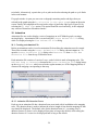
3.3.2 Saving a Graph XML File
To save the current graph as a zipped archive either select the Save Graph menu item from
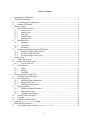
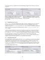
the File menu or click the toolbar button. The dialog shown in Figure 1 will appear. The
radio buttons in the Nodes and Edges to Save and Other Information to Save
frames let you tell FCModeler what you want to save. If you have made subgraphs you can save
either the information in the top subgraph only (the one visible on the screen), in all the
subgraphs, or all of the information in FCModeler’s memory, regardless of whether it is visible
or not. The Contents file information frame lets you set general information about
the data in the graph, if you wish. When finished click the Save button on this screen which will
make a standard file selection dialog appear, in which the location and name to save the new
archive can be specified.
Figure 1. Save graph option dialog. This dialog lets you save information about the graph and to specify
which part of the graph information to save.
3.3.3 Saving an Image of the Graph
FCModeler can create an image file (JPEG, SVG, or PNG format) of the displayed graph. This
may be useful for including the graph in a document or web page. The entire active graph (not
just the portion of it visible on the screen, if it is zoomed) is included in the image, and it is saved
with the visible color and shape properties. To create an image of the graph view, select the
Save Graph Image menu item from the File menu, and indicate the file and format
desired.
8
4
Graph Layout
To view a graph, a graph layout algorithm must compute positions of the node and edge figures.
Many different graph layout algorithms exist. FCModeler currently uses Dot and GEM to
compute its layouts.
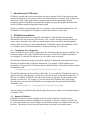
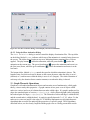
4.1 Simple Dot Layout
There are two types of layout that can be computed by Dot. The first is a generic layout called
the Simple Dot Layout. When a graph is opened in FCModeler Simple Dot Layout is applied by
default. It can be applied at any time by selecting Dot Layout from the Layout menu.
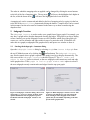
Figure 2 shows a graph layout done using the simple dot layout.
Figure 2. Example of the simple dot layout using a small graph.
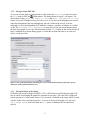
4.2 Rank-Cluster Dot Layout
Dot can also be used to compute a more customized layout. Based on their values of certain
node properties, the node figures can be placed on horizontal ranks or into clusters. When a
graph is open in FCModeler, select the Dot Rank-Cluster Layout menu item from the
Layout menu. An open file dialog box is shown in which a layout XML file must be selected
(see below). Figure 3 below shows the same graph as in Figure 2 using the rank-cluster layout.
9
Figure 3. Rank-cluster dot layout.
4.2.1 Layout XML File
The ranks and clusters for the rank-cluster layout are specified in a layout XML file. The XML
file used in the layout for Figure 3 is shown below:
<?xml version="1.0" standalone="yes"?>
<!DOCTYPE layout [
<!ELEMENT layout (rank*, cluster*)>
<!ELEMENT rank (atom*, composite*)>
<!ATTLIST rank
label CDATA #REQUIRED>
<!ELEMENT cluster (atom*, composite*, cluster*)>
<!ATTLIST cluster
label CDATA #REQUIRED>
<!ELEMENT atom EMPTY>
<!ATTLIST atom
property CDATA #REQUIRED
value CDATA #REQUIRED>
<!ELEMENT composite ((atom | composite), connective, (atom | composite))>
<!ELEMENT connective EMPTY>
<!ATTLIST connective
type (and | or) #REQUIRED>
]>
<layout>
10
<rank label="rank1">
<atom property="type" value="type1"/>
</rank>
<rank label="rank2">
<atom property="type" value="type2"/>
</rank>
<rank label="rank3">
<atom property="type" value="type3"/>
</rank>
<cluster label="AandB">
<composite>
<atom property="label" value="a"/>
<connective type="or"/>
<atom property="label" value="b"/>
</composite>
</cluster>
<cluster label="EandF">
<composite>
<atom property="label" value="e"/>
<connective type="or"/>
<atom property="label" value="f"/>
</composite>
<cluster label="OnlyG">
<atom property="label" value="g"/>
</cluster>
</cluster>
</layout>
The <rank> tag is used to specify the nodes that should be placed in a certain horizontal rank.
Each rank has a label, specified by the label attribute, which is shown on the left-hand side of the
graph view. Nodes are selected using the same type of XML as in the property-to-visualattribute mappings (see section 7).
Similarly, the <cluster> tag is used to specify nodes to place in a cluster. Each cluster is
surrounded by a rectangle and has a label, specified by the label attribute, which is shown on the
upper-left of the cluster. The <cluster> tag uses the same node selection mechanism as the <rank>
tag. <cluster> tags can be nested inside each other, creating nested clusters as shown in clusters
EandF and OnlyG above.
4.3 GEM Layouts
The GEM family of layouts are also available in FCModeler. These are GEM, AGEM, and
FastGEM, and are derived from code developed by the Tulip project (www.tulip.org).
GEM is the standard layout in the GEM family. It can handle disconnected graphs but takes the
longest to run; the quality is good and consistent. AGEM runs much faster than GEM but does
not handle disconnected graphs well and the quality is only fair and much more inconsistent.
FastGEM uses AGEM to do the initial layout then GEM to refine the layout, making quality
layouts more consistently than AGEM.
4.3.1 GEM
This is the standard layout as detailed in "A Fast Adaptive Layout Algorithm for Undirected
Graphs" by Frick, Ludwig and Mehldau. This code is a Java translation of the Frick's
11
implementation in C code. GEM turns every node into an electron and every edge into a
stretched spring and places a gravitational force at the barycenter of the layout. A node is
attracted to all nodes adjacent to it and is repelled by every node whether or not it is connected
by an edge. In addition, there is an attractive gravitational force between each node and the
barycenter of the graph. GEM has three main loops: the insertion loop, the arrangement loop, and
the optimization loop. The insertion loop is where the nodes are initially placed. The closer a
placement is to the final layout, the faster the arrangement loop runs. The arrangement loop does
most of the work getting the nodes to their final positions. Following the example of Tulip, we
did not implement the optimization loop.
Figure 4: Example of a GEM layout, using the same graph as in Figure 2 and Figure 3.
4.3.2 AGEM
This is the "new" spring embedder algorithm that differs significantly from GEM. It uses much
of the framework of the GEM algorithm, but the heart of it is different. AGEM removes the
repulsive force between pairs of nodes, reverses the direction of the gravitational force to make it
repulsive, and retains the attractive spring forces between adjacent nodes.
AGEM gives a layout that is similar to the regular GEM, but does it much faster. Because of the
lack of repulsion between nodes, an unlucky initial random layout could leave many nodes
bunched together. Also, the reversed gravity tends to push singletons and disconnected
subgraphs away from the barycenter. This increases the global temperature of the layout causing
it to use its maximum allowed number of iterations instead of stopping early due to settling of
the graph.
12
4.3.3 FastGEM
FastGEM is a compromise designed to give the more consistent quality of GEM while retaining
some of the speed of AGEM. FastGEM uses AGEM to do an initial layout and GEM to finish.
AGEM replaces Frick's insertion loop. With a layout that is often near to the final layout, the
regular GEM algorithm runs significantly faster. If there are disconnected pieces of the graph,
the AGEM algorithm will take a long time to complete, so any speed advantages over GEM will
be lost.
5
Interacting with the Graph View
5.1 Selecting Nodes and Edges
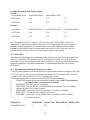
Multiple nodes and/or edges can be selected at any given time, as shown in Table 1. Selected
nodes and edges are highlighted in the graph: nodes by a yellow border and edges by a thick red
line.
Table 1. Methods of selecting nodes and edges.
To Select
Individual node or edge
Multiple nodes and/or edges
Multiple nodes and/or edges
Do This Action
click on a node or edge
hold the Ctrl key and click on multiple nodes and/or edges
click and drag around multiple node and/or edges
5.2 Node Operations
All operations that change node information are performed using the Modify Nodes dialog
(Figure 5). This dialog is opened by selecting Modify then Nodes from the top FCModeler
menu.
5.2.1 Modifying Node Information
Open the Modify Nodes dialog (Figure 5). Only one node’s information can be changed at a
time. Select the node whose information you want to modify in the graph, then click the Get
Node button on the Modify Nodes dialog. FCModeler will read all the available information
about the node and display it on the Modify Nodes dialog. Different parts of the dialog will
be active depending on the types of files that are present in the open graph archive. Only
information for files that are present can be changed.
The Node Properties section of the Modify Nodes dialog will always be active, since
this information is present for every node in every FCModeler graph (see Figure 6). The unique
ID is set by FCModeler and can not be modified, but all the other properties can be changed. The
name box is the name that will be used to label the node on the graph. The type box is the
node’s type. All the node types in the graph are listed in the drop-down box. You can select one
of the existing node types for this node’s type or make a new one by typing in the type box and
pressing the return key. Similarly, the location box lists all the existing node locations, so
you can select an existing location or type in a new one.
13
The molecule ID field can be modified if necessary. FCModeler uses the molecule ID of
each node to keep track of information about a molecule that may be shared among several
nodes. For example, there may be one node in the graph to represent glucose in the cytosol and
another node to represent glucose in the nucleus. The location and unique ID of these two nodes
will be different but the molecule IDs will be the same, since they both represent glucose. The
molecule ID of any node can be viewed by right-clicking the node and selecting Node
Properties, or by using the Identify Node dialog. To change a node’s molecule ID click
the change button to the right of the molecule ID box on the Modify Nodes dialog. This
will make the molecule ID box editable so that a new value can be entered.
The Modify Nodes dialog in Figure 7 shows the dialog’s appearance when the graph archive
contains pathways, index, and extended files. All parts of the dialog are editable. Abbreviations
for the node are listed in the abbreviation(s) list, and synonyms in the synonym(s)
list. For both lists new items can be added by clicking the add new button and existing items
deleted by clicking the delete button after selecting the desired item. The Pathways
Information section lists all pathways in the archive that the node is not a member of in the
left-side box and all the pathways that the node is a member of in the right-side box. Change the
pathway membership by selecting the desired pathway name and clicking the arrow keys.
After the desired node properties have been changed click the Save Changes button to save
the changes. Clicking the Cancel button will undo any changes that have been made since the
node was selected.
5.2.2 Adding New Nodes
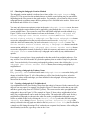
Open the Modify Nodes dialog (Figure 5). Click the Add New Node button. A unique ID
will be generated automatically, but you must specify the molecule ID, name, and type for the
node. Other node information (such as its location, abbreviations, or pathway membership) may
be set if desired, see section 5.2.1 for detailed instructions. When all of the information has been
entered click the Save Changes button. The new node will be added to the upper left part of
the graph. After the Add New Node button is clicked the new node must be added; you can not
cancel the operation.
14
Figure 5. Modify Nodes dialog.
This dialog is used to add new
nodes, delete nodes, and change
the information associated with
existing nodes. It is opened by
selecting Modify then Nodes
from the top FCModeler menu.
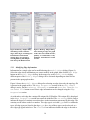
Figure 6. Modify Nodes dialog
after selecting a node. The graph
archive does not contain an index,
pathway, or extended file, so only
the Node Information section
is active.
Figure 7. Modify Nodes dialog
after selecting a node. The graph
archive contains the index,
pathways, and extended file, so all
sections of the dialog are active.
5.2.3 Deleting Existing Nodes
The Modify Nodes dialog is also used to delete nodes from the graph. All edges attached to
the node must be deleted before the node is deleted; a node can not be deleted if it has edges. To
delete edges please refer to section 5.3.3. To delete an existing node open the Modify Nodes
dialog (Figure 5) and select the node(s) to delete in the graph. Then click the Delete
Selected Nodes button in the Modify Nodes dialog. A message box will appear, asking
you to confirm that you wish to delete the selected node(s). If you click OK the node(s) will be
permanently removed from the visible graph and the archive; the node will no longer appear in
any subgraph. Deleting a node can not be undone.
5.3 Edge Operations
All operations that change edge information are performed using the Modify Edges dialog
(Figure 8). This dialog is opened by selecting Modify then Edges from the top FCModeler
menu.
15
Figure 8. Modify Edges dialog.
This dialog is used to add new
edges, delete edges, and change the
information associated with
existing edges. It is opened by
selecting Modify then Edges
from the top FCModeler menu.
Figure 9. Modify Edges dialog
after selecting an edge. The graph
archive does not contain an index,
pathway, or extended file, so only
the Edge Information section
is active.
5.3.1 Modifying Edge Information
Information for a single edge can be modified using the Modify Edges dialog (Figure 8).
Select the edge whose information you want to modify in the graph, then click the Get Edge
button on the Modify Edges dialog. In the same way as the Modify Nodes dialog,
different parts of the Modify Edges dialog will be activated depending on what files are
present in the open graph archive.
Figure 9 shows the Modify Edges dialog after selecting an edge when only the topology file
is present in the graph archive. The Edge Properties section of the Modify Edges
dialog is active, but the Pathways Information section and describe changes in
extended file button are not. Basic edge information can be changed using the Edge
Properties section.
As with nodes, each edge has a unique ID assigned by FCModeler. This unique ID is displayed
in the Edge Properties section but can not be modified. The certainty field is used to
indicate the degree of certainty researchers have in the interaction represented by this edge. The
certainty can be either words or a number. The edge type is set in the type field. As with node
types, all edge types are listed in the edge type box. Any of these types can be selected, or a
new edge type typed in the box. The directed box indicates whether the edge is directed or
16
not; only “yes” and “no” are the only allowed values. Finally, the strength field holds a text
or numerical value indicating the strength of the reaction represented by the selected edge.
The head and tail node of the selected edge can also be changed using the Edge
Information section of the Modify Edges dialog. The head node is the node that the
edge points to; the tail node is the node the edge comes from. To change the head or tail click
the node in the graph that you want to be the new head or tail, then click the corresponding
select node button on the dialog. The dialog will show the new node’s name in the head
node or tail node box, but the graph will not be updated until the changes are saved.
If a pathways file is present the Pathways Information section of the Modify Edges
dialog will be active. This section works in the same way as the Pathways Information
section of the Modify Nodes dialog; see 5.2.1, Modifying Node Information.
5.3.2 Adding New Edges
To add a new edge to the graph, click the Add New Edge button in the Modify Edges
dialog. FCModeler will automatically create a new unique ID for the edge, but you need to set
the certainty, strength, type, and directed fields. You must also select the nodes to use as the head
and tail for the new edge. After setting the properties for the new edge click the Save
Changes button and the new edge will appear in the graph.
5.3.3 Deleting Existing Edges
To delete an existing node open the Modify Edges dialog (Figure 8) and select the edge(s) to
delete in the graph. Then click the Delete Selected Edges button in the Modify
Edges dialog. A message box will appear, asking you to confirm that you wish to delete the
selected edge(s). If you click OK they will be permanently removed from the visible graph and
the archive; the edges will no longer appear in any subgraph. Deleting an edge can not be
undone.
5.4 Moving Nodes and Edges
Nodes can be moved by selecting them and dragging them with the mouse. Attached edges will
move with the selected nodes. Edges can be moved by selecting the edge then manipulating the
control points which are shown as blue boxes (see Figure 10). The node and edge positions can
be saved in a coordinate file for reloading, otherwise they will be lost whenever a layout is
applied or if the graph is closed.
17
Figure 10. Selected
edge showing control
points.
5.5 Zooming
FCModeler supports zooming of the graph view to examine the graph in varying levels of detail.
To enlarge the graph select View then Zoom In from the top menus or click the toolbar
button. To zoom out, either select View then Zoom Out from the top menu or click the
toolbar button.
5.6 Finding a Particular Node
In very large graphs it can be difficult to locate specific nodes. Nodes can be searched by using
the Find Node dialog (Figure 11). This dialog will let you find a node, after which FCModeler
will select it in the graph and move the display so that the node is in the center. The dialog is
opened by selecting View then Find Node from the top FCModeler menu.
If you know the exact name of the node it can be found by typing its name in the Name of
node to locate box on the Find Node dialog and clicking the Find button.
Alternatively, one or more nodes can be identified using the Identify Node dialog. Open the
dialog by clicking the Identify Nodes button, then identify the node(s) you wish to find in
the normal way (see section 6, Using the Identify Node Dialog for more information). Click
OK in the Identify Node dialog to close it, then Find on the Find Node dialog.
18
Figure 11. The Find Node dialog. This dialog is used to locate one or more nodes in the
visible graph.
6
Using the Identify Node Dialog
The Identify Node dialog (Figure 12 and Figure 13) is used throughout FCModeler to
identify nodes. It does not alter the graph or graph view in any way, but rather lets you indicate
which nodes you are interested in even if the nodes are not present on the screen. For example,
you may wish to make a subgraph of a graph that is too large to view. The Identify Node
dialog lets you select the nodes that you want to include in the subgraph.
The Identify Node dialog consists of two halves. The right side contains a list, while the
left side has three frames. The boxes checked on the left side of the screen determine what is put
in the list on the right side. The right side lists node identifiers; which identifiers are included is
set by the left side boxes.
The Identify Node dialog will have different amounts of information depending on the
files present in the graph archive. For example, Figure 12 shows the Identify Node dialog
when a small graph that only contains a topology file is loaded. The graph in Figure 13 has an
index and pathway file so the Pathways frame contains items and the Properties frame has
a synonyms entry.
By default, when the Identify Node dialog is opened it lists the names of all nodes in the
graph. This state is shown in Figure 13: the node names option in the Properties frame is
checked, all rows in the Locations frame are checked, and all rows in the Pathways frame
are checked. You can restrict the list of nodes to certain pathways and/or locations by
unchecking the corresponding boxes in the Locations and Pathways frames. Additionally,
you can view nodes by type, synonym, or molecule ID in addition to name. Click the Update
View button after checking or unchecking boxes on the left side of the dialog to update the node
list.
Nodes are identified by selecting their identifiers in the list on the right side and clicking the OK
button. You may select as many nodes in the list as you wish; hold the Ctrl key while clicking
to select multiple entries, or the Shift key to select blocks of entries. Depending on the graph,
selecting one row in the Identify Node list may identify more than one node in the graph.
Many nodes may share the same synonym, name, or molecule ID.
19
Figure 12. The Identify Node dialog. This dialog
is used to identify nodes by name, type, location,
pathway, or other properties.
7
Figure 13. Identify Node dialog when a large
graph with pathways and index information is
loaded.
Node and Edge Properties
The nodes and edges of the graph have multiple properties associated with them. Node
properties include type (e.g. gene, RNA, protein) and location; edge properties include type (e.g.
conversion, regulation, catalyst) and strength. Properties provide information about what the
nodes and edges of the graph represent. Each node and edge of the graph has a value for each
property.
7.1
Viewing Properties with the Property Viewer
The Property Viewer (Figure 14) shows the property values of all selected nodes and
edges. To open the Property Viewer, select the Property Viewer menu item from the
Interaction menu or right-click on an item in the graph and select Detailed
Properties from the pop-up menu. As nodes and edges are selected and deselected in the
graph the Property Viewer window will update to show the information for the currently
selected nodes and edges.
The Node Table and Edge Table frames on the left side of the Property Viewer
display basic information for each selected node and edge. Clicking on a row in either table will
cause detailed information about that row’s node or edge to appear in the right side window.
What information is displayed depends on how much data about the node or edge is available in
the graph archive. FCModeler will display all available information, including information from
the topology, index, pathway, and extended files. If reference information is available web links
may be shown in the panel, which will open your web browser when clicked.
20
Figure 14. Property Viewer showing property values of selected nodes and edges. The right side shows
detailed information for the node whose row is selected in the Node Table: AT1G16350.
7.2 Viewing Properties of a Single Item
You can also view the property information for any particular node or edge without using the
Property Viewer. Right-click the node or edge and select Node Properties (or Edge
Properties, if an edge) from the pop-up menu. A window will appear, as shown in Figure 15.
This window shows the same information as the right side panel of the Property Viewer.
21
Figure 15. Dialog showing the properties for a single node. The properties for this node include a reference
link, which opens the default web browser when clicked.
8
The Mapping Editor
The Mapping Editor (Figure 16) is used to change the appearance of a graph, either of individual
nodes and edges or of all nodes and edges in a particular category. For example, all nodes in the
graph of type gene can be displayed with an elliptical node shape, or one edge can be displayed
in red. To open the Mapping Editor, either select the Mapping Editor menu item from the
View menu or click the toolbar button.
Mapping rules are statements that describe the appearance changes to be made to the graph, such
as: If edgeType is equal to enzyme then connector end is circle, If nodeType is equal to
polypeptide and location is equal to unknown then node outline color is red, or If id is equal to
A154d then node fill color is blue. These rules are created using the dropdown lists on the Edge
Properties, Node Properties, Pathway, and Selection tabs of the Mapping
Editor.
The Mapping Editor allows the following attributes to be changed:
• nodes: node fill color, node outline color, node shape
• edges: connector end, line color, line thickness, line type
22
Figure 16. The Mapping Editor after creating one mapping rule based on edge properties.
8.1 Using the Node Properties and Edge Properties tabs
The particular nodes and edges to be altered can be selected based on their properties. For
example, consider a graph that has several types of nodes and edges, such as the one shown in
Figure 16. Suppose we want to color all edges of type enzymatic reaction blue. To do this, we
click on the Edge Properties tab, and create the mapping rule If edgeType is equal to
Enzymatic reaction Then line color is blue, as shown in Figure 16. Click the Apply button to
view the effect the mapping rule has on the graph while leaving the Mapping Editor open. To
change the appearance of all nodes with a particular characteristic, such as their location or type,
the Node Properties tab is used in the same manner.
In more detail, begin creating a new mapping rule by clicking either the Edge Properties
or Node Properties tab, depending on if the node or edge appearance should be changed.
The top If dropdown list box contains a list of all of the edge (or node) properties that are
present in the current graph. Select the property that you wish to base the rule on, such as the
edgeType. When a property is selected in the first box the second dropdown list is automatically
filled with all of the values for that property present in the graph. Select the value that you want
included in the rule, such as Enzymatic reaction.
You may also create a compound rule involving two conditions, such as If certainty is equal to
indirect evidence or edgeType is equal to Catalysis then line color is red, indicate the connector
(or or and) from the list at the end of the first line, and create the second rule from the second
property and value boxes. The mapping editor illustrated in Figure 17 is configured to make this
compound rule.
The mapping rule illustrated in Figure 18 uses a color, light blue, which is not included in the list
of basic colors. Colors not shown in the dropdown list can be indicated by selecting other as the
23
color in the value list. A standard color selection dialog will appear, from which any color can
be chosen.
Figure 17. Mapping editor configured to create the
compound mapping rule If certainty is equal to
indirect evidence or edgeType is equal to Catalysis then
line color is red.
8.2
Figure 18. Mapping editor configured to create the
mapping rule If nodeName is equal to ADP then node
fill color is light blue.
Using the Selection tab
The Selection tab of the Mapping Editor (Figure 20) allows mapping rules to be created for
the nodes and/or edges that are selected in the graph. First select nodes and/or edges in the
graph, then click the Get Selected Nodes and Edges button. The number of nodes and
edges selected will be displayed in the label to the left of the Get Selected Nodes and
Edges button.
After the nodes and edges have been selected, using either method you can indicate the desired
appearance of the selected objects. The same attributes are changed in the same way as on the
Node and Edge Properties tabs. By default FCModeler will make mapping rules for both
the nodes and edges. If you only want to change the node or edge attributes deselect the
corresponding check box. Finally, click the Add Mapping Rules button, which will create
mapping rules describing the appearance of each selected node and edge.
8.3
Using the Pathway tab
If the graph archive contains a pathway file, the Pathway tab (Figure 19) can be used to change
the appearance of all nodes and/or edges in a particular pathway. All pathways present in the
graph archive are listed in the pathways box by default; select the list pathways in
window only option to restrict the list to those pathways that have at least one member in the
visible graph. As with the Selection tab, mapping rules can be made for the nodes or edges
by checking the appropriate boxes.
24
Figure 19. Pathway tab of the Mapping Editor. All
edges in the Acetyl-CoA Biotin network will be changed
to have no connector end. The node appearance will
not be changed since create node rules was
unchecked.
Figure 20. Selection tab of the Mapping Editor.
Mapping rules for eight nodes and six edges will be
created; the edges will be green and the nodes will be
diamond-shaped.
8.4 Using the Mapping Editor Buttons
After each mapping rule has been created click the Add Mapping Rule button on the tab.
The mapping rule will then be converted into FCModeler format and added into the list of
mapping rules on the bottom portion of the mapping editor.
To view the effect of the current mapping rules click either the Apply or OK button at the
bottom of the mapping editor. The Apply button will apply the mapping rules to the graph in
FCModeler without closing the mapping editor. The OK button will apply the rules and close the
mapping editor.
The Revert button at the bottom of the mapping editor deletes all mapping rules that may have
been applied and returns the graph to its default appearance. The Cancel button will close the
mapping editor without applying any of the additional mapping rules that are present. Any rules
that were already applied will be unaltered, however.
The list of mapping rules present in the mapping editor can be saved to an external file by
clicking the Save Mapping File button. The list of rules can later be loaded by clicking the
Load Mapping File button. Saving and loading mapping rule files allows the appearance
of a graph to be quickly altered without creating mapping rules each time. Many mapping files
can be created for each graph, but only one can be displayed at a time.
8.5 Advanced Mapping Rule Manipulation
Mapping rules are managed with the buttons in the Mapping Rules frame at the bottom of
the mapping editor. All active mapping rules are listed in the large box. An individual rule can
be deleted by clicking on the rule to highlight it then clicking the Delete Selected Rule
button; all rules can be deleted with the Delete All Rules button. If no default mapping
file is set in the main FCModeler preferences, clicking Delete All Rules then Apply will
have the same effect as clicking the Revert button.
Mapping rules are applied in the order in which they are listed in the mapping editor list box (top
first, bottom last). The order in which the rules are applied may affect the appearance of the
graph. For example, one rule, such as If certainty is equal to high then line color is blue, will
change all edges with high certainty to blue. Another rule, such as If edgeType is equal to
biochemical reaction then line color is red, will change some edges to red. Some edges may be
both of high certainty and the type biochemical reaction. If the first rule is applied before the
second, lines that are both high and biochemical reaction will be red, but if the second is applied
before the first these lines will be blue.
25
The order in which the mapping rules are applied can be changed by clicking the arrow buttons
to the left of the list of mapping rules. The up arrow, , will move the highlighted rule higher in
the list, while the down arrow, , will move the highlighted rule lower in the list.
A mapping rule can be constructed and added to the list of mapping rules by typing it in the box
to the left of the Manual Entry button and clicking the button. Complex rules can be created
in this manner, but the rules must be formatted in the same way as those created using the
dropdown lists.
9
Subgraph Creation
The Subgraph Creator is used to make a new graph from a bigger graph. For example, you
may have a graph archive that has thousands of nodes and edges. This graph is too big to display
at once. Instead, you use the Subgraph Creator to tell FCModeler which part of the graph you
want to see, such as all nodes and edges within 4 steps of a particular node. FCModeler will
make this new graph (a subgraph of the graph archive) and open a new window to show it.
9.1
Starting the Subgraph Creator dialog
Open the Subgraph Creator dialog by selecting Graph then Create Subgraph from
toolbar button. The Subgraph Creator
the top FCModeler menu or by clicking the
may also be started when a graph is opened if the graph is too big to display automatically. The
first screen of the Subgraph Creator is shown in Figure 21. The all nodes and
edges in memory option is selected, so the new subgraph could contain any node and edge
in the graph archive. If the graph in active graph window ONLY option is selected
the new subgraph can only contain nodes and edges from the top open graph.
Figure 21. Subgraph Creator dialog's first screen.
The graph in active graph window ONLY
option is disabled because no graph was open in
FCModeler when the Subgraph Creator was
started.
26
Figure 22. Main Subgraph Creator screen. This
screen lets you indicate how you want choose the
nodes and edges in the subgraph. Some of these
options may be unavailable, depending on the files
present in the graph archive.
9.2 Choosing the Subgraph Creation Method
The subgraph creation method is indicated on a frame of the Subgraph Creator dialog
(Figure 22). This screen lists the methods that are available; some options may be unavailable,
depending on the files present in the graph archive. For example, you will not be able to create
subgraphs based on pathway name unless a pathways file is included in the archive. Select one of
the methods and click the Next button.
You may only choose one option at a time in the main Subgraph Creator screen, but more
than one subgraph creation method can be applied by going through the Subgraph Creator
screen multiple times. The screens for each of the individual subgraph creation methods (e.g.
Figure 23) have a set of three buttons in a frame at the bottom: Create subgraph now,
Create subgraph then choose another method, and Choose another
method without making a subgraph now. The Create subgraph now button
creates the subgraph based on the previous selection and closes the Subgraph Creator
while the other two buttons take you back to the main Subgraph Creator screen. The
Choose another method without making a subgraph now button cancels the
current action, while the Create subgraph then choose another method button
creates the subgraph but instead of showing it, holds it in memory and returns you to the main
Subgraph Creator screen. In this way a subgraph can be made by any combination of
options.
For example, you may have a large graph archive that has nodes from multiple pathways. You
may wish to view all of the nodes in a particular pathway that are within 5 steps of a particular
node. You can do this by first creating a subgraph by pathway name, then clicking the Create
subgraph then choose another method button, then creating a subgraph by P
neighborhood.
9.3 Creating a Subgraph by Pathway Name
If by pathway name is selected on the main Subgraph Creator screen the dialog will
change to look like Figure 23. All of the pathways will be listed in the large box; select the
pathway(s) whose nodes and edges you want included in the subgraph. As many pathways as
desired can be selected.
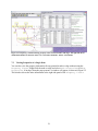
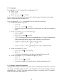
9.4 Creating a Subgraph by P Neighborhood
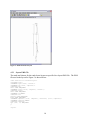
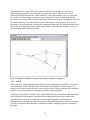
A p neighborhood is the set of nodes p steps from the node(s) of interest. Nodes connected by an
edge are one step apart. For example, the graph in Figure 25 shows the nodes that are one (red)
and three (green) steps from AT3G58610 (yellow). The screen used to make p neighborhood
subgraphs is shown in Figure 24. The example in Figure 25 shows the p neighborhood of one
node, but p neighborhoods can be made for many nodes. The nodes that will be used for the p
neighborhood subgraph are shown in the white list on the p neighborhood subgraph screen.
Nodes are added to this list by clicking the Identify Nodes (each node selected using the
Identify Node dialog), Named Pathway, Current Selection in Graph (the
node(s) selected in the top graph are added to the list), or Read from File (the file should be
a simple text file listing the unique ID of each node on a separate line) buttons. After adding the
desired node(s) to the list, type the p value in the P box.
27
Figure 23. Subgraph Creator dialog's pathway
subgraph screen. The screen is set up to create a
subgraph of all nodes in the glucose 1-phosphate
metabolism pathway.
Figure 24. Subgraph Creator dialog's p
neighborhood subgraph screen. The screen is set up
to create a subgraph of all nodes within two steps of
the pyruvate node.
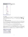
Figure 25. P neighborhood of node AT3G58610 (in
yellow). The red node is the first neighbor, the
reaction node the second, and the green nodes the
third.
Figure 26. Subgraph Creator dialog's edge type
subgraph screen.
9.5 Other Subgraph Creation Options
The by identifying nodes directly or from a path/cycle option provides
an interface for several subgraph creation options. All of these options let you specify the nodes
that you want to include in the subgraph; edges connecting these nodes will also be included. If
you know which nodes you want to include you can use the Identify Node dialog or
FCModeler will read them from a text file (plain text, each line of the file a unique ID of a node
28
to include). Alternatively, a particular cycle or path can be selected using the path or cycle finder
in the usual manner.
If a graph window is open you can create a subgraph containing nodes and edges that you
selected in the graph using the by selection in the open graph option on the main
screen. Finally, the subgraph can be restricted to edges of particular edge types (Figure 26) by
selecting the by edge type option. This option should be used cautiously, or the subgraph
may consist of numerous unconnected nodes.
10 Animation
Animation files are used to display a series of mappings on an FCModeler graph, creating a
moving display. An animation file is created using the Create Animation File dialog,
while it is displayed using the View Animation File dialog.
10.1 Creating an Animation File
Before an animation can be viewed an animation file describing the animation must be created.
These files are made using the Create Animation File dialog, shown in Figure 27. To
open the Create Animation File dialog select Interaction then Create New
Animation File from the top FCModeler menu.
Each animation file consists of a series of steps, each of which is made of mapping rules. The
Add New Step to Animation button on the Create Animation File dialog brings
up the Mapping Editor, which is used in the regular manner (see 8 The Mapping Editor) to
construct the mapping corresponding to that step.
Figure 27. The Create Animation File dialog, as appears when it first opens.
10.1.1 Animation File Duration Factors
Each step in an animation file has a duration factor associated with it in addition to the mapping
rules. The duration factor is used to indicate the relative length of time that the mapping for that
step should be displayed. The default value for the duration factor is 1, so setting a step’s
duration factor to 4 causes it to be displayed four times as long as the default, while setting the
duration factor to 0.5 causes it to be displayed half as long as the default.
29
The duration factor for a step can be set when the step is added (by typing it in the Duration
factor for new step box before the Add New Step to Animation button is
clicked) or by selecting the step in the list of steps on the Create Animation File dialog,
typing the new duration in the Duration factor for new step box and clicking the
Update button.
10.1.2 Order of Steps in the Animation
The steps in the animation file will be shown in the order in which they appear on the Create
Animation File list. Each new step is added to the bottom of the list, so the steps will be
displayed in the order in which they were created unless the order is altered.
To alter the order in which the steps will be shown select the step to move, then click the up
or down
arrow. A step can be deleted by clicking the Delete Selected Step
button after the step has been selected.
10.1.3 Saving the Animation File
After all of the steps have been added to the animation file, and are shown on the Create
Animation File dialog in the correct order the animation file can be saved by clicking the
Save Animation File button. This button will cause a standard save dialog box to be
displayed, in which the desired location and name for the animation file can be specified. As
with mapping files, as many animation files as desired can be created for each graph archive, and
the animation files are stored as separate files, not part of the graph archives.
10.2 Viewing an Animation File
Animation files for a graph can be viewed after they are created. The speed of the animation can
be altered while it is being viewed, and the animation can be paused at any time.
10.2.1 Opening an Animation File
The animation specified in an animation file is viewed using the Show Animation dialog, as
shown in Figure 28. To open the Show Animation dialog select Interaction then View
Animation File from the top FCModeler menu. A standard file open dialog will appear, in
which you should navigate to and select the animation file that you wish to view. FCModeler
will read the file and open the Show Animation dialog.
30
Figure 28. The Show Animation dialog, used to display and control animations.
10.2.2 Using the Show Animation Dialog
The Show Animation dialog is used to control the display of animation files. The top slider
on the dialog, labeled Frame, indicates which step of the animation is currently being shown on
the screen. The slider always begins at step zero, indicating that no mappings have yet been
applied. The play button ( ) starts the animation, while the pause button ( ) pauses the
animation at the current step. The go-to-front button ( ) pauses the animation and resets it to
the first (zero) frame, while the go-to-end button ( ) pauses the animation and resets it to the
last frame.
The bottom slider, labeled Delay, controls the speed at which the animation is shown. The
length of time for which each step is shown on the screen decreases when the delay is set to 1
(shortest) or 2, and increases when the delay is set to 4 or 5 (longest). The relative duration of
each step set by the duration factor remains constant, even when the delay is altered.
11 Graph Theoretic Operations
Graphs are well-studied mathematical objects and an entire area of mathematics, called graph
theory, exists to study their properties. A graph consists of two parts: a set of objects called
nodes (or vertices) and a set of relations between nodes called edges. If a graph is undirected, its
edges are unordered pairs of vertices, e = {u, v} = {v, u} , while a directed graph (called a digraph)
has ordered pairs for edges, e = (u, v) ≠ (v, u ) . The first node of a directed edge is called the tail,
and the second node is called the head. A graph is typically denoted G = (V , E ) , where V is the
node set (or vertex set) and E is the edge set. FCModeler implements several graph theoretic
algorithms that are useful for analyzing the properties of a specific graph. These algorithms,
described below, are also closely coupled with the graph view to visually present their results.
31
11.1 Subgraphs
For a digraph D = (V, E), a digraph H is a subdigraph of D if
• V ( H ) ⊆ V ( D)
• E ( H ) ⊆ E ( D)
• E ( H ) = {(v, u ) ∈ E ( D ) v, u ∈ V ( H )}
In other words, all of the nodes of H must be in D, all of the edges of H must be in D, and the
edges of H must have both end-nodes in H.
For a given digraph D = (V, E), a subdigraph H can be created in several ways:
• Given a set of nodes W ⊆ V (D)
o V (H ) = W
o E ( H ) = {(v, u ) ∈ E ( D ) v, u ∈ V ( H )}
o H consists of some subset of nodes of D and all edges in D with both end-nodes in
that set
• Given a set of nodes W ⊆ V (D) and an integer p
o V ( H ) = N Dp [W ]
o E ( H ) = {(v, u ) ∈ E ( D) v, u ∈ V ( H )}
o
N Dp [W ] is defined as the closed p-th neighborhood of W. Saving W and all nodes
visited on directed paths of length p from each node in W forms the set.
o
N [W ] = N
p
D
+p
D
p
p
[W ] ∪ N [W ] = ∪ N (W ) ∪ ∪ N D−i (W )
−p
D
i =0
+i
D
i =0
⎞
⎛
N D+ p (W ) = N D+ ⎜⎜ N D+ ( p −1) (W ) − ∪ N D+i (W )⎟⎟ and N D− p (W ) is defined similarly.
i =0
⎠
⎝
Given a set of edges B ⊆ E (D )
o V ( H ) = {v ∈ V ( D) v ∈ (v, u ) ∈ E ( H )}
p −1
o
•
•
o E(H ) = B
o H consists of all end-nodes of the edges in B and all of the edges in B.
Given a set of nodes W ⊆ V (D) and a set of edges B ⊆ E (D)
o V (H ) = W
o E ( H ) = {(v, u ) ∈ B v, u ∈ V ( H )}
o H consists of all nodes in W and all edges in B with both end-nodes in W.
11.2 Strongly Connected Components
A digraph D is strongly connected if every vertex of D is reachable from every other vertex of D.
The strongly connected components (SCC’s) of a digraph D are the maximal strongly connected
subdigraphs of D. The SCC’s are useful to analyze, because every node in an SCC is reachable
from every other node in the same SCC.
32
The algorithm for finding the SCC’s of a digraph D is extremely simple and is based on two
modifications of depth-first search (DFS).
1. Compute an acyclic ordering of the nodes using DFS.
2. Compute the converse D’ of D.
3. Perform DFS on D’, using the ordering from Step 1. Each DFS tree is a SCC of D.
To find the strongly connected components of a graph in FCModeler, select the Find
Strongly Connected Components menu item from the Graph menu. After performing
the above algorithm, FCModeler lists the SCC’s (Figure 29). Clicking on an SCC in the list
selects its nodes and edges the graph.
Figure 29. Example of selecting strongly connected components.
11.3 Finding and Viewing Cycles
A path in a digraph is an alternating sequence of nodes and edges, v1e1v2e2v3 … vk-1ek-1vk, such
that tail( ei ) = vi , head( ei ) = vi +1 , and all nodes are distinct. A path can be viewed as starting at
node v1 and following edges through the graph until node v k is reached. If v1 = v k , the path is
called a cycle.
The Find Cycles dialog (Figure 30) is used to find cycles in FCModeler. The dialog is
opened by clicking the toolbar button or selecting Graph then Find Cycles from the top
menu. The dialog will find all cycles in the graph, or you can restrict it to searching for cycles of
a particular length or containing particular nodes. To restrict the cycles to particular nodes, click
either the Identify node or Select node buttons. The Max cycle length box is
used to set the maximum cycle size (in number of edges). Click the Find cycles button to
find cycles of the length and containing the nodes you specified, or click the Find All
Cycles button to find all cycles in the graph.
33
11.4 Finding and Viewing Paths
A path is the collection of nodes and edges that lead from one node to another node. The Find
Paths dialog (Figure 31) in FCModeler searches for all paths of the specified length between
two nodes. Open the Find Paths dialog by clicking the toolbar button or selecting Graph
then Find Paths from the top menu.
Set the starting and ending node for the path using either the Identify Node dialog (by
clicking the appropriate Identify Node button) or by selecting the nodes directly in the
graph (select the node then click the appropriate Select Node button). The maximum path
length is set to unlimited by default; change this to the maximum path length you want (each
edge is counted as one unit of length) and click the Find Paths button to perform the search.
All paths found will be put in the list box; click on the path name to view it in the graph.
Figure 30. The Find Cycles dialog. Three cycles
containing the node u-1 (blue) were found. The
selected cycle (u-1, a, b, v) is highlighted in the graph.
Figure 31. Find Paths dialog. The dialog found all
paths from node u-1 to node z (in pink). One path was
found and highlighted.
11.5 Clustering Cycles with SOM
Cycles obtained from directed graphs may be similar to each other based on their node and edge
content. Thus, clustering algorithms may be used to find natural groups of similar cycles. Prior
to clustering, a distance metric and generalized set median must be defined for the objects to be
clustered. Several possible representations for the cycles are discussed, including strings, graphs,
and weighted sets. Weighted sets are chosen because of the simplicity of the associated metric
and median. Self-organizing maps are used to find clusters of cycles obtained from a directed
graph. This approach is implemented using the JSOMap package for self-organizing maps.
The map view window (Figure 32) shows a grid of small graphs, one for each unit of the map.
The map view window is opened by selecting Graph then Run SOM on Cycles after the
Find Cycles dialog has been used to find all of the cycles in a graph. Each window of the
34
map view dialog represents the model for that particular map unit. The models are the
generalized median of the set of cycles assigned to that map unit. Figure 32 shows an example
of a 4-by-4 SOM results in the map view window.
Figure 32. Map view window showing results of the SOM algorithm. Each graph shows the model of the
corresponding map unit, which is the generalized median of the cycles assigned to that map unit.
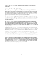
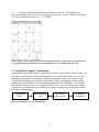
12 Using R for Complex Visualization
Experimental profiling data can be visualized in FCModeler graphs using R. Figure 33 shows the
procedure of visualizing user data with FCModeler. First, import the data and process it by R, a
language and environment for statistical computing and graphics (http://www.r-project.org).
Then perform data processing, which includes preprocessing, color mapping, and producing
mapping rules for FCModeler. The communication between R and FCModeler is via an XML
based protocol: Simple Object Access Protocol (SOAP, http://www.w3.org/TR/soap/). Finally,
visualize the experimental data in FCModeler by creating mapping rules to change the colors of
particular nodes and edges.
Experimental
Data
Data Processing
in R
Java to R
linker (SOAP)
Figure 33. Visualizing user data with FCModeler.
35
FCModeler
Visualization
12.1 R Configuration
R is freely available at http://www.r-project.org/; download and install the most recent version
for your system if you do not already have a copy. Two R packages must also be installed:
tkrplot and XML. These packages are also freely available for download, either from CRAN
via the R website or from within R itself (select Packages then Install Packages from
the top menu).
To configure R to work with FCModeler, system environment variables must be set.
• In Windows, set the R_HOME environment variable: Click Start then Control Panel.
In the Control Panel click the System icon then the Advanced tab. On the
Advanced tab click the Environment Variables button. In the dialog click the New
button in the System Variables frame, then create a new environment variable pointing
to the R installation location, e.g. Variable name: R_HOME and Variable Value:
C:\Program Files\R\rw2010. Click OK in the dialogs to close them.
• In Linux users can follow similar steps except setting the R_HOME environment variable.
• The R functions have not been tested on Macintoshes. For now, please use a Linux or
Windows environment on your Mac, and follow instructions above.
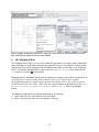
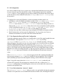
12.2 View Expression Data and Test the Configuration
To test the connection open the 8Pathways.zip graph archive, one of the sample graphs that came
with FCModeler. Then open the Animation Control Panel by selecting
Interaction then View Animation from Script from the top menu. A file open
dialog will appear, from which you can select an R script to view. Several test files are included
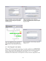
with the FCModeler distribution; select animation.R. The Animation Control Panel
(Figure 34) should then open (Please check the background of the desktop, if the GUI does not
pop up.). This dialog is used to send information to R. You can set what kind of node or edge
properties are sent to R, and filter the nodes or edges by properties, pathways or selection. Click
the Run Script button and FCModeler will send information to R and run the selected R
script.
If the Animation Control Panel does not appear check if R is running and if R has the
two necessary packages (tkrplot and XML) installed. It may be helpful to close FCModeler
and R (including any R processes that might be running), restart FCModeler and try again.
Figure 34 (top left corner) shows the Animation Control Panel produced by the
animation.R R script file. Do not change any settings but click the OK button; the Show
Animation dialog (Figure 28) should appear, so you can view the data in the context of the
metabolic and regulatory map.
12.3 Use of the Animation Control Panel
The Animation Control Panel dialog is used to view and modify the data the animation
is based on. We plan to have several additional functions available soon, including the ability to
36
open multiple files. For example, you may wish to view proteomic data together with microarray
data. Also, we want to add GUIs for data processing, clustering, and mapping to FCModeler.
12.3.1 Input Data frame
Select a microarray, proteomic or metabolomic data file. Select an Experiment Information File,
describing your experimental samples (RNA, protein, or metabolites) and how they were
obtained. For the data formats, please refer to the example at the end of the document (section
14, Appendix: R Script File Formats).
12.3.2
Data Preprocessing Setting frame
This frame is used to select subset of the data. Usually, there are multiple replicates, genotypes,
time points or treatments in a data file, user can select specific subgroups of them, as shown in
Figure 34. Checking the Fold Change between GenoType box will show the fold
change between different genotypes (WT and mutant in the example data). Checking the
Average Replicates box will show the average expression of the replicates. The Scale
of Expression Value can be set to either Log (default) or Unlog. For microarray data,
the program will automatically determine the data’s original scale by checking the data’s
maximum amplitude (if minimum amplitude is less than 0, the data is in Log scale), then transfer
the data to the scale the user specified. The option to Standardize Each Profile to 0
mean and 1 variance is provided. This is useful for finding correlational patterns. Without
standardizing, we cannot see the similar changing patterns among nodes because their
amplitudes are not comparable with each other.
12.3.3 Output Setting frame
If the Use Equal Time Interval box is checked the time interval between animation
frames will be equal, otherwise real time intervals (computed based on the sample time) will be
used. The Set Animation Colors button opens a dialog to change the default animation
colors. As shown in Figure 34, the default animation is based on the three color mapping: the
high value color (red), the middle value color (yellow) and the low value color (blue). Check the
Save Animation File option to output an animation file for future use. The saved
animation file can be loaded into FCModeler later using the Show Animation File dialog
(see section 10.2.2, Using the Show Animation Dialog).
12.3.4 View Data Profiles
The user can view the data profiles by clicking the View Expression Profiles option
under the View Data menu item, as shown in Figure 35. A GUI will show all the entity names
of the selected type (By default, it will show all the RNA names), in which you can select part or
all of them and view their profiles. By clicking a profile it will be highlighted and the name of
corresponding entity will be shown in the status bar and highlighted in the list box, as shown in
Figure 35. You may also highlight the profiles by double-clicking the name in the list box. The
profiles can be standardized or in usual scale.
37
When users open a new data file, the “View
Info” button will become “Create Info”.
Users can create new experiment information
Figure 34. Animation Control Panel dialogs.
38
Figure 35. View Profiles dialog.
12.3.5 Data preprocessing details used in animation.R
In order to visualize and interpret the data more effectively, the data is preprocessed.
• Trim the outliers. It is very possible there are outliers, which will skew the color mapping.
Here we trim expression value over 98% of the global maximum expression value and less
than 2% of the global minimum expression value.
• Linearly scale the trimmed expression values to the range [0, 1]. The “1” value corresponds
to the high value color, “0.5” value corresponds to the median value color (for fold change
data, “0.5” value corresponds to no change) and the “0” corresponds to the low value color.
12.4 Write your own R script
The example script (animation.R) is located in the fcmodeler/scripts/ directory. Referring to this
script may assist you in developing your own R animation scripts. Another sample script is
39
network.R, which returns the graph structure and displays it as a subgraph, the same as the
original graph.
12.4.1 Entry point
The entry point of FCModeler to an R script is the function ‘main'. FCModeler provides two
parameters to R script, FCMNodeList and FCMEdgeList, which are the first two arguments of
the function ‘main'. Both FCMNodeList and FCMEdgeList are “list” class in R. Their names are
the node and edge attribute names. For FCMNodeList, it includes all the node attributes: id,
molId, nodeName, nodeType, location and etc. For FCMEdgeList, it includes all the edge
attributes: id, head, tail, strength, edgeType, certainty etc. A script may or may not use all these
information in its production of mapping rules.
12.4.2 Return Values
Return values of main are in a list data structure. At present, it supports two types of returns. One
is the mapping rules, which maps the graph in different colors and node shapes. The other is the
graph structure, which creates a subgraph in FCModeler. The parameter type determines which
type of return it is.
When type is mapping or without type information, the return structure is of the form:
list(type=”mapping”, mappingRules=mappingRules, exptName=exptName,
timePoint=timePoint, duration=duration, refresh=0), where
•
•
•
•
•
mappingRules is a list in which the mapping rules are stored. This field is mandatory.
duration is the time difference between two sets of mapping rules. If the difference is
negative or the time information is not available, just use unit duration. By default, it is 1.
refresh is used to tell FCModeler whether to refresh the graph display before applying the
new mapping rules. By default, it is 0; this means it will add the new mapping rules on the
old graph.
exptName is a list of Affymetrix experiment names at each time point or experiment. By
default, it uses a format like “experiment 1”.
timePoint is the time point of each experiment. If not provided, it uses the experiment index
number.
When type is graph the return structure is of the form:
list(type='graph', nodeAttName=nodeAttName, edgeAttName=edgeAttName,
nodeInfo=nodeInfo, edgeInfo=edgeInfo)
•
•
•
nodeAttName lists the node attribute names included in nodeInfo matrix;
edgeAttName lists the edge attribute names included in edgeInfo matrix;
nodeInfo is a matrix. Each row represents one node; each column represents one particular
node attribute, such as “id”, “nodeName”, or “location.” These are the same attributes as the
FCModeler topology file. The “id” field is required.
40
•
edgeInfo is a matrix. Each row represents one edge; each column represents one particular
edge attribute, such as “id”, “from”, “to”, or “edgeType.” These are the same attributes as the
FCModeler topology file. The “id”, “from” and “to” fields are required.
13 References
13.1 Publications relating to FCModeler
Cox, Z. (February 28, 2002). JSOMap: a Java-based Self-Organizing Map package.
http://jsomap.sourceforge.net. Date accessed: June 18, 2002.
Dickerson, J. A., D. Berleant, et al. (to be published in 2002). Creating and Modeling Metabolic
and Regulatory Networks Using Text Mining and Fuzzy Expert Systems. Computational Biology
and Genome Informatics. C. H. Wu, P. Wang and J. T. L. Wang, World Scientific.
Dickerson, J. A., D. Berleant, et al. (2001). Creating Metabolic Network Models using Text
Mining and Expert Knowledge. Atlantic Symposium on Molecular Biology and Genome
Information Systems and Technology (CBGIST 2001), Durham, North Carolina.
Dickerson, J. A., Z. Cox, et al. (2001). Creating Metabolic and Regulatory Network Models
using Fuzzy Cognitive Maps. North American Fuzzy Information Processing Conference
(NAFIPS), Vancouver, B.C.
13.2 Open Source Code Used in FCModeler
Dot graph layout routine from the Graphviz package of AT&T
(http://www.research.att.comsw/tools/graphviz).
Diva framework graph nodes and edges (http://www.gigascale.org/diva/)
Java SDK (http://java.sun.com/)
Tulip GEM Routine for graph layout (http://www.tulip-software.org)
14 Appendix: R Script File Formats
The data file is a tab-delimited text file. Excel files can be easily saved as tab-delimited text files.
14.1 Microarray DATA
The first row is the sample name list (e.g., sample 1, sample 2, ,,,).
Data columns: The first column is the locus name (eg. AT2G02010), the next data columns are
the experimental values for each sample.
At present, “animation.R” can automatically detect and delete the extra spaces in the row and
column names. It can handle both format 1 and 2. It can also automatically detect duplicated row
names (for microarray data, one locus Id could appear several times in a single chip.) and output
the duplicated list.
41
Example Microarray data flat file format:
Format 1:
At.StarchSD1.Wt.0L At.StarchSD1.Wt.0L
At.StarchSD1.Wt.0L
AT5G11160
6.64
6.41
7.12
AT2G02010
4.47
4.27
5.37
“Any Name”
At.StarchSD1.Wt.0L
At.StarchSD1.Wt.0L
At.StarchSD1.Wt.0L
AT5G11160
6.64
6.41
7.12
AT2G02010
4.47
4.27
5.37
Format 2:
Here, At.StarchSD1.Wt.0L is sample 1, and 6.64 is the value for this sample. In this case,
AtStarchSD1 is the experiment name of replicate1, WT is the genotype, 0L is the timepoint.
Format 1 is the default format of R produced data, such as Bioconductor normalized data.
Format 2 is the default format of the data transferred from Excel file. In this case, the first
element of first row can be any name, our program just ignores this element.
14.2 Other Data
Other data, like fold-change data, metabolomic data and proteomic data, can be formatted in the
same way. (Proteomic files currently can only be displayed according to locus ID. Work on
visualization of protein modifications and protein complexes is in progress. Metabolomic data is
displayed regardless of subcellular compartment. Compartmentalization function is being
developed.)
14.3 Experiment information file format (an example)
# This is a tab separated text file that describes an experiment in which two genotypes (ACL and
# WT) were grown under short day conditions, and sampled at 11 time points (WT) or 3 time
# points (ACL) during a diurnal cycle. Two replicates were made.
# Each experiment group is composed of the UNIQUE-ID and its attributes.
#
UNIQUE.ID includes the experiment name and sample name. It MUST be identical to
the sample name on the microarray data file;
#
#
TIMEPOINT is the time point of each sample;
#
GENOTYPE They are WT(var. Columbia) and ACLA1(antisense ACLA1, Fatland,
#
Nikolau, Wurtele, 2004) in this example;
#
TREATMENT (in this case, there is no treatment, so column is left blank)
#
REPLICATE Two replicates are available in this case.
#
AUTHORS: Carol Foster, Li Ling, Martha James, Alan Myers, Basil J. Nikolau,
#
Eve Syrkin Wurtele
UNIQUE.ID
TIMEPOINT
GENOTYPE
At.StarchSD1.Wt.0L
0
WT
42
TREATMENT REPLICATE
1
At.StarchSD1.Wt.0.5L
0.5
WT
1
At.StarchSD1.Wt.1L
1
WT
1
At.StarchSD1.Wt.4L
4
WT
1
At.StarchSD1.Wt.0D
8
WT
1
At.StarchSD1.Wt.0.5D
8.5
WT
1
At.StarchSD1.Wt.1D
9
WT
1
At.StarchSD1.Wt.4D
12
WT
1
At.StarchSD1.Wt.6D
14
WT
1
At.StarchSD1.Wt.8D
16
WT
1
At.StarchSD1.Wt.12D
20
WT
1
At.StarchSD2.Wt.0L
0
WT
2
At.StarchSD2.Wt.0.5L
0.5
WT
2
At.StarchSD2.Wt.1L
1
WT
2
At.StarchSD2.Wt.4L
4
WT
2
At.StarchSD2.Wt.0D
8
WT
2
At.StarchSD2.Wt.0.5D
8.5
WT
2
At.StarchSD2.Wt.1D
9
WT
2
At.StarchSD2.Wt.4D
12
WT
2
At.StarchSD2.Wt.6D
14
WT
2
At.StarchSD2.Wt.8D
16
WT
2
At.StarchSD2.Wt.12D
20
WT
2
At.StarchSD1.ACLA1.1L
1
ACLA1
1
At.StarchSD1.ACLA1.0.5D 8.5
ACLA1
1
At.StarchSD1.ACLA1.4D
12
ACLA1
1
At.StarchSD2.ACLA1.1L
1
ACLA1
2
At.StarchSD2.ACLA1.0.5D 8.5
ACLA1
2
At.StarchSD2.ACLA1.4D
ACLA1
2
12
43