Download R-integration package - Agilent Technologies

Agilent GeneSpring GX –
R-integration package
Installation and Application
Guide
2
GeneSpring GX – R integration package
1
Table of Contents
1
2
Table of Contents..........................................................................................................................3
Introduction and summary ............................................................................................................3
2.1
Introduction...........................................................................................................................3
2.1.1
R....................................................................................................................................4
2.2
What is new in this release....................................................................................................4
2.3
Summary ...............................................................................................................................4
3 The GeneSpring GX External Program Interface.........................................................................5
3.1
How the EPI works ...............................................................................................................5
3.2
Setup .....................................................................................................................................5
3.2.1
Upgrading from a previous version of the R integration package ................................6
3.2.2
Installation procedure....................................................................................................6
3.3
Post-installation modifications............................................................................................16
3.3.1
WINDOWS.................................................................................................................16
3.3.2
UNIX/MacOSX ..........................................................................................................17
3.4
Creating External Programs using R...................................................................................19
3.4.1
WINDOWS: GS_exec_R.bat......................................................................................19
3.4.2
UNIX/Mac OS X: GS_exec_R.sh...............................................................................22
3.4.3
Create the R script.......................................................................................................22
3.4.4
Create the External Program definition in GeneSpring GX .......................................23
3.4.5
Running the External Program....................................................................................26
3.4.6
Using the Graphical User Interface for R ...................................................................27
4 The GeneSpring R Package ........................................................................................................28
4.1
Installing the GeneSpring package .....................................................................................28
4.2
The GeneSpring functions ..................................................................................................33
5 Appendix A. Complete R examples............................................................................................34
5.1
Box plot...............................................................................................................................34
5.2
Filter on CV ........................................................................................................................34
5.3
gapFilter ..............................................................................................................................35
5.4
DifferentialExpression-LPE................................................................................................36
5.5
DifferentialExpression-SAM ..............................................................................................37
5.6
Power of ANOVA...............................................................................................................38
5.7
Q value with plots ...............................................................................................................39
5.8
Z score normalization .........................................................................................................41
2
2.1
Introduction and summary
Introduction
Gene Expression analysis has become a very mature field and there are many different
analyses that can be performed using gene expression data. Many scientists develop their
own algorithms that will help them understand their data and allow them to answer their
scientific questions. Many of the custom analyses are developed in specialized packages
like R, SAS, Matlab JMP etc. and many users would like to be able to integrate their
specialized algorithms into a common platform like GeneSpring GX.
The GeneSpring GX External Program Interface (EPI) will allow a user to integrate any
program or algorithm in a seamless way, giving the user the flexibility to perform whatever
analysis they would like, in the familiar environment, without having to manually save the
expression data outside of GeneSpring GX and perform the analysis and re-import the data
into GeneSpring GX. With the EPI this can all be done in such a way that the end-user will
never have to even see that an analysis is performed outside of GeneSpring GX.
GeneSpring GX – R integration package
3
Many scientists have chosen to perform the specialized analyses in the Language R in
special R scripts, and the GeneSpring GX-R integration package was developed to facilitate
the incorporation of those R scripts into the GeneSpring GX environment. The integration of
the R language into GeneSpring GX is only one of the examples showing the versatility of
GeneSpring GX to interact with other analysis tools and we hope that you will find this
information useful in your future expression analysis research.
2.1.1
R
R is a statistical computing language which is freely available. It is rapidly gaining traction
within the Bioinformatics world and especially in the Gene Expression analysis field since it
has a high statistical analysis need.
The R program can be obtained for many platforms and this document will cover the
integration of R and GeneSpring GX for Windows and Unix platforms. For more information
on R visit the web site:
http://cran.us.r-project.org/
2.2
What is new in this release
This is the second release of the GeneSpring GX-R Integration package and a number of
new features and bug fixes are part of this release:
1) Upgrade R to version 2.1.0
The version of R that is included in this release is version 2.1.0, released 18-Apr-2005.
This contains numerous changes and bug fixes. For a complete list of the new features
in R 2.1.0 consult the R web site.
2) Added box plot script
Added new example script to create a simple Box Plot in R.
3) Removed RMA scripts
Since GeneSpring GX 7.1 has native support for RMA and GC-RMA analysis of CEL
files, there is no need for a R version of the RMA scripts and therefore have been
removed from this version.
4) All of the scripts were updated to work with GeneSpring GX R library version 2.0.0
BioConductor 1.6 contains a new version of the GeneSpring GX library (version 2.0.0)
and the example scripts were changed to work with GeneSpring GX library version
2.0.0.
GeneSpring GX library version 1.0.x used the GeneSpring GX systematic name as row
names for many of the expression matrices and certain characters that are valid
characters in systematic names (Namely #) are not valid characters for Matrix row
names, leading to some conversion issues. GeneSpring GX library 2.0.0 stores the
gene names in a special slot, allowing for any character to be used as a systematic
name.
NOTE: R scripts written to use GeneSpring GX library 1.0.x ARE NOT
COMPATIBLE with this new version of the GeneSpring GX library.
5) All of the scripts were updated to work with R version 2.1.
The contents of certain libraries have been changed in R version 2.1.0 and the example
R scripts have all been updated to work with R version 2.1.
2.3
Summary
This document contains a description of how be able to run R scripts from within the
GeneSpring GX Interface. The document describes the installation of the R integration
package provided by Agilent and contains numerous examples of functional R scripts that
perform useful analysis.
4
GeneSpring GX – R integration package
This document is also available from our website at:
http://www.chem.agilent.com/cag/bsp/SiG/Downloads/pdf/gs_r_doc
.pdf
3
3.1
The GeneSpring GX External Program Interface
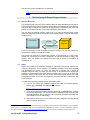
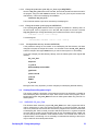
How the EPI works
The GeneSpring GX External Program Interface (EPI) will allow GeneSpring GX to start an
external program and provide this program with the data to be analyzed. When the program
is finished with its analysis, the results will be passed back to GeneSpring GX, which will
present the user with the results in the familiar GeneSpring GX Interface.
The only thing the external program needs to do, is to read the standard input stream
(STDIN) and write the results to the standard output stream (STDOUT) and GeneSpring GX
will do the rest.
Genespring
STDIN
Your
program
STDOUT
If it is not convenient to read the STDIN and write to STDOUT you can also redirect the
input/output to a file and read that file in stead.
The program can either be a command line program, a JAVA program or a HTTP POST
request, but the principle is the same. GeneSpring GX will send a stream of data to the
program which will perform the analysis and send back a stream of information to
GeneSpring GX.
3.2
Setup
Agilent has provided an R-integration package for GeneSpring GX that can install all the
necessary components on your computer. The installation package can be simply dropped
onto GeneSpring GX version 6.1◊ which will install the R package and a number of
examples which will help you create your own library of R scripts that will expand the
capability of GeneSpring GX. For those users that already have a copy of R, we have also
provided a version of the installer that only contains the GeneSpring GX-specific part of the
R integration package. This version may require the user to edit two files to indicate the path
to the R program.
To install the R-integration package perform the following steps:
1) If you do not already have installed R and will not install the complete Windows
version (gs_r_winall.zip), download and install R from:
http://cran.us.r-project.org/
2) If you will not install the complete Windows version (gs_r_winall.zip which contains
the complete R package), you need to install the R GeneSpring GX Library from the
CRAN/BioConductor site, by using the built-in download packages functionality in R
(See Chapter 4 for more information).
3) Download one and only one of the GeneSpring GX-R Integration package ZIP file
from our web site, listed below:
◊
The installation of GeneSpring-R integration package via the drag and drop interface of the ZIP file, is only compatible
with version 6.1 of GeneSpring and later. For information about upgrading to version 6.1 or later, released Nov-2003 see
the Agilent website at http://www.agilent.com/chem/genespring/ or chose Update GeneSpring from the Help menu.
GeneSpring GX – R integration package
5
For WINDOWS including R program (2.1.0) and BioConductor + GeneSpring library:
http://www.chem.agilent.com/cag/bsp/SiG/Downloads/zip/gs_r_win
all.zip
OR for WINDOWS NOT including R program or any library:
http://www.chem.agilent.com/cag/bsp/SiG/Downloads/zip/gs_r_win
.zip
OR for UNIX NOT including R program or any library:
http://www.chem.agilent.com/cag/bsp/SiG/Downloads/zip/gs_r_uni
x.zip
4) Drag the ZIP file onto any open window of GeneSpring GX or use Menu “File>Open GeneSpring Zip”
5) Change the path for the scripts and/or R program (See section 3.3)
6) Change the permission on the execution scripts (UNIX only, See section 3.3.2)
7) PRESTO! You are done…It’s that simple to get started with R in GeneSpring GX!
If you need more help in the installation procedure, see the next section “Installation
procedure”.
3.2.1
Upgrading from a previous version of the R integration package
This is the second release of the GeneSpring GX-R Integration package, and if a previous
version of the package has been installed, most of the files will be overwritten by the new
versions of the programs, so if any changes have been made that need to be retained,
make copies of the changes so they could be implemented in the new versions if required.
3.2.2
Installation procedure
This section describes the steps involved in the installation of the GeneSpring GX-R
Integration package.
3.2.2.1
Installing R
If you did not install R before or did not use the complete Windows package
(gs_r_winall.zip) you would need to install the R program. See the download and
installation instructions at http://cran.us.r-project.org/ on how to install R for your platform.
3.2.2.2
Installing BioConductor
The GeneSpring GX-R integration package can be used most optimally with the R package
BioConductor. The BioConductor package is not required for most functionality of the
GeneSpring GX R integration package, but it is highly recommended to obtain the
BioConductor package. If you do not already have the BioConductor library and will not
install the complete Windows package (gs_r_winall.zip) you need to install the
BioConductor package separately. More information about the installation of the
BioConductor package can be found at:
http://www.bioconductor.org/
3.2.2.3
Installing GeneSpring GX R library
The GeneSpring GX-R integration package uses a special R library called “GeneSpring
GX”. This library performs most of the actual conversion functions and is required for the
use of the GeneSpring GX-R integration package. This library is now part of the
BioConductor release 1.6 and later. For information about installation of the “GeneSpring
GX” R library see Chapter 4.
The R library is called “GeneSpring GX” allowing the library to be loaded in an R session by
the command:
6
GeneSpring GX – R integration package
library(GeneSpring)
Note the capitalization. See Section 4.1 for more information about the functions in the
library GeneSpring GX or check the vignette in R.
3.2.2.4
Installing GeneSpring GX-R Integration package into GeneSpring GX
Starting with version 6.1, GeneSpring GX can install any GeneSpring GX related item with a
special Drag and Drop interface that will make it easy to install new functionality and data
into GeneSpring GX. With the Drag and Drop ZIP technology, you will be able to install new
pathways, new genomes, new physical maps, new scripts and external programs and
Agilent will use the new Drag and Drop interface to continue to enhance the functionality of
GeneSpring GX via this interface. The GeneSpring GX-R integration package is the one of
the first examples of this technology.
If the ZIP file is not already present on your machine, download the file from the
GeneSpring GX Extra section of our website http://www.agilent.com/chem/genespring/ or
use the links provided in the previous section. There are a number of versions of the
installer, depending on your platform (WINDOWS or UNIX/MacOSX) and whether you
would like to include R or not.
Open GeneSpring GX and once the window for the Genome is opened, go to the location
where you saved the ZIP file and select the file and drag the file onto the open window of
GeneSpring GX. In this case it does not matter which Genome you have opened; it will work
with any Genome∇. Alternatively, use the menu item “File->Open GeneSpring GX Zip” to
open the ZIP file.
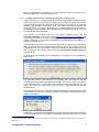
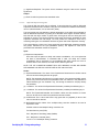
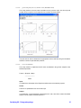
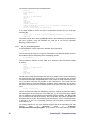
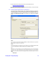
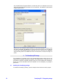
Once you dropped or opened the file in GeneSpring GX, a dialog box will be presented as
shown below:
The dialog box shows a short description of the Installer and it will inform the user that
GeneSpring GX will quit after the installation is complete. Press <No> if you are not ready to
quit GeneSpring GX yet, press <Yes> if you would like to proceed. Depending on the
version of the zip file you downloaded, the text may be slightly different from the one
displayed above.
The installation will take a few minutes and after the installation is complete, another dialog
box will be shown, informing you that the installation was successful and GeneSpring GX is
ready to be shut down.
Occasionally, it is possible that GeneSpring GX will first display a message that certain files
will be overwritten and you can still abort the installation procedure at this point by clicking
∇
For other Drag and Drop files in the future, like Pathways etc. it may make a difference which Genome you drop the
ZIP file on.
GeneSpring GX – R integration package
7
the <No> button if you feel that you would like to double check that the files you are about
the overwrite can indeed be updated.
The first time you install the GeneSpring GX-R Integration package you should NOT see
this message, since all files are supposed to be new.
3.2.2.5
New External Programs
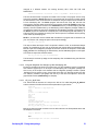
Once you have installed the GeneSpring GX-R Integration package, the next time you start
up GeneSpring GX you should see a number of new items in the External Programs and
the Scripts section.
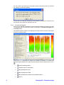
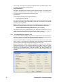
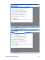
The External programs section of GeneSpring GX should contain a number of extra items
as shown in the figure below:
There are 8 or 11 (Depending on whether you installed on Windows or on UNIX) new
External Programs defined in the folder External Programs that are indicated with a R icon (
):
8
1.
Boxplot (WINDOWS ONLY)
2.
Calculate Power on Interpretation
3.
DifferentialExpression-LPE
4.
DifferentialExpression-SAM
5.
DifferentialExpression-SAM w plots (WINDOWS ONLY)
6.
Filter CV
GeneSpring GX – R integration package
7.
gapFilter
8.
Qvalue
9.
Qvalue with plots (WINDOWS ONLY)
10.
Z score normalization
Each of the external programs is implemented as an R external program via the EPI.
Although the external programs can be run from the External Programs section, we have
also provided a number of scripts that implement the R scripts that will give the user a little
more control over how the R scripts should be run and will also show the integration of the R
external programs into the scripting environment of GeneSpring GX
3.2.2.6
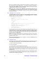
New Scripts
The installer has also created a new folder in the Scripts folder called “R scripts” that
contains eight new scripts:
The scripts are called:
1) Box plot
2) Calculate power
3) Differential Expression using LPE
4) Differential Expression using SAM
5) Filter on CV
6) Gap Filter
7) Q value from 1-way ANOVA results
8) Q value with plots from 1-way ANOVA results
9) Z-score Normalization
The scripts contain extensive notes explaining how they work. A short overview of the
purpose of the scripts is given below.
GeneSpring GX – R integration package
9
3.2.2.6.1
Box plot
This script will create a box plot in a graphical R window.
Input:
(1) Experiment Interpretation
The interpretation for which the box plot needs to be created.
Knobs:
No Knobs are defined for this script.
Output:
This script does not produce any output that can be stored in GeneSpring GX.
3.2.2.6.2
Calculate power
This script calculates the Power for each gene, based on the variance within and between
the groups (conditions) of the Interpretation.
Input:
(1) Experiment condition
The input of this script is an Experiment Interpretation containing at least two conditions
and each condition should have at least 2 replicates (to be able to calculate the
variation within the group).
Knobs:
10
GeneSpring GX – R integration package
(1) SignificanceRequired: The power will be calculated using this value as the required
significance.
Output:
(1) Gene List with the power as the associated value
3.2.2.6.3
Differential Expression using LPE
This script will filter the genes with an adjusted P value less than the cutoff for differential
expression between the two conditions, using the Local Pooled Error Model as described by
Jain et. al, Bioinformatics, Vol 19, 1945-1951 (2003).
The local pooled error test attempts to reduce dependence on the within-gene estimates in
tests for differential expression, by pooling error estimates within regions of similar intensity.
Note that with the large number of genes there will be genes with low within-gene error
estimates by chance, so that some signal-to-noise ratios will be large regardless of mean
expression intensities and fold-change. The local pooled error attempts to avert this by
combining within-gene error estimates with those of genes with similar expression intensity.
The script produces a Gene List of those genes that show differential expression between
two groups, indicated as the input parameters (knobs). The adjusted P value will be
provided as the associated number for the genes.
Input:
(1) Experiment Interpretation
Since the script will perform a dChip and Lowess normalization, it is not required that
the data is prenormalized. If normalized data is used, the dChip and Lowess
normalization will be performed on pre-normalized data which should not have an
adverse effect on the outcome, but could result in different gene lists.
NOTE: THE LPE ALGORITHM CANNOT DEAL WITH MISSING VALUES AND GENES
WITH MISSING VALUES WILL NOT BE USED IN THE CALCULATION.
Knobs:
(1) ExperimentParameter: The name of the Experimental Parameter that contains values
that can be used to distinguish the two groups.
NOTE: The parameter name should not contain spaces. If the parameter DOES contain
spaces, only use the first word of the parameter name. For instance, in the parameter is
called "Disease type" use "Disease" only, Use enough characters to uniquely identify
the parameter.
(2) Condition1: The value of the Experimental Parameter (condition) that defines group 1
(3) Condition2: The value of the Experimental Parameter (condition) that defines group 2
NOTE: The ExperimentParameter and Condition values are case sensitive so ensure
that you use the correct case for the parameter name and values.
(4) PvalueCutoff: The P value cutoff value. Only genes with an (adjusted) P value of this
value or less will be returned.
(5) MulTestingCorrection: Name of the multiple testing correction method to be used to
adjust the P value.
Possible values for the Multiple Testing corrections are:
For false discovery rate (FDR):
"BH" : Benjamini & Hochberg (1995) (Default)
"BY": Benjamini & Yekutieli (2001)
"none" or "no": No Multiple Testing Correction
GeneSpring GX – R integration package
11
Output:
(1) GeneList: Those genes that are differentially expressed between the two groups and
have a adjusted P value below the cutoff (PvalueCutoff)
3.2.2.6.4
Differential Expression using SAM
The program will calculate the d value for differential expression between the two groups,
using the SAM (Significance Analysis of Microarrays) method, implemented in R, as
described by Tusher, V.G., Tibshirani, R., and Chu, G. (2001). Significance analysis of
microarrays applied to the ionizing radiation response, _PNAS_, 98, 5116-5121.
NOTE: A LICENSE IS REQUIRED FOR COMMERCIAL USE OF SAM. Non-commercial
use is permitted. For more information on how to obtain a license for commercial use of
SAM see http://otl.stanford.edu/industry/resources/sam.html
The script produces a Gene List of those genes that show differential expression between
two groups, indicated as the input parameters (knobs). The d value will be provided as the
associated number for the genes.
The script will launch the R program and will also produce a plot in the R interface that can
be used to determine a good FDR and d value cutoff values. When the R program is closed,
the resulting gene list can be saved in GeneSpring GX.
Input:
(1) Experiment Interpretation
The normalized experiment data will be used.
Knobs:
(1) ExperimentParameter: The name of the Experimental Parameter that contains values
that can be used to distinguish the two groups.
NOTE: The parameter name should not contain spaces. If the parameter DOES contain
spaces, only use the first word of the parameter name. For instance, in the parameter is
called "Disease type" use "Disease" only, Use enough characters to uniquely identify
the parameter.
(2) Condition1: The value of the Experimental Parameter (condition) that defines group 1
(3) Condition2: The value of the Experimental Parameter (condition) that defines group 2
NOTE: The ExperimentParameter and Condition values are case sensitive so ensure
that you use the correct case for the parameter name and values.
12
GeneSpring GX – R integration package
(4) FDR: The False Discovery Rate as a fraction (0 to 1).
The FDR will be used to determine the d value cutoff values of what is to be considered
a significantly differentially expressed gene.
Output:
(1) GeneList: Those genes that are differentially expressed between the two groups and
result in a FDR as set by the FDR knob.
The associated value for the gene list will be the d value as calculated by the SAM
method
3.2.2.6.5
Filter on CV
This script will filter the chosen Interpretation on the Coefficient of Variation. (CV =
100*Standard Deviation/Mean)
The CV values can be calculated on either the Raw data (Default) or the Normalized data.
The script produces a Gene List of those genes that show a CV value less than the
CV_cutoff parameter in a specified number of Conditions.
Input:
(1) Experiment Interpretation
(2) The starting gene list
Knobs:
(1) CV_cutoff: The minimum Coefficient of Variation in percent
(2) Matching_conditions: The minimum number of Conditions that have to show a CV value
less than CV_cutoff.
The Matching conditions parameter is either a whole number or a fraction. When a
whole number, it indicates the absolute number of conditions that need to pass; when a
fraction, it indicates that fraction of conditions that need to pass.
For example, a setting of Matching_conditions of 4 indicates 4 conditions need to pass,
while 0.5 indicates that half of the conditions need to pass.
(3) Data_to_use: The type of data to use.
Possible values are "Raw" or "Normalized" ("R" or "N" can also be used).
Default = "Raw"
Output:
(1) GeneList: Those genes that pass the filter cutoff and the number of matching conditions.
3.2.2.6.6
Gap Filter
This script implements the BioConductor filter "gapFilter".
The "gapFilter" looks for genes that might usefully discriminate between two conditions
(possibly unknown at the time of filtering). To do this we look for a gap in the ordered
expression values. The gap must come in the central portion (we exclude jumps in the initial
'Prop' values or the final 'Prop' values). Alternatively, if the Inter Quartile Range (IQR) for the
gene is large that will also pass our test and the gene will be selected.
Input:
(1) Experiment Interpretation
The NORMALIZED data for each of the genes, for each Condition will be used.
GeneSpring GX – R integration package
13
Knobs:
(1) Gap: The minimal Gap required between the high and low values for the gene to pass
the filter
(2) IQR: Inter Quartile Range. When a gene shows a IQR of at least this value it will also
pass the filter
(3) Prop: The proportion of values that should be excluded from Gap and IQR calculations.
If less than 1, the value is taken as a ratio, if 1 or higher, the number represents the
number of conditions on each side of the sorted values to be disregarded.
Output:
(1) GeneList: Those genes that pass one or both of the filters.
3.2.2.6.7
Q value from 1-way ANOVA results
Script calculates a 1-way ANOVA on the selected Gene List and Experimental Parameter. It
will calculate the Q value and will return a Gene List of those genes that have a Q value
below the cutoff value (Qcutoff). The Q value is a P value that is corrected for the multiple
tests that are performed in the ANOVA. It computes the multiple testing correction factor (ε)
to limit the false discovery rate. For a given gene i with P value pi, new P value (Q value)
becomes pi+ε.
The statistical methodology mainly comes from:
Storey JD. (2002) A direct approach to false discovery rates.
Journal of the Royal Statistical Society, Series B, 64: 479-498.
See http://faculty.washington.edu/~jstorey/qvalue/ for more info.
Input:
(1) Starting Gene List
(2) Experiment condition
The Experiment condition should have at least 2 conditions.
Knobs:
(1) Groups Specification: The name of the Experimental parameter to be used in the 1-way
ANOVA. The parameter should be entered using the GeneSpring GX specific format:
{Experimental parameter name}:{*}
(2) Q_cutoff: The cutoff value for the Q value. Only genes with a Q value at or below this
value will be returned
(3) bootstrap: Parameter will determine the method for automatically tuning the parameter
in the estimation of pi0, the proportion of true null hypotheses. Set to 'yes' or 'y' for
choosing the 'bootstrap' method, Use 'no' or 'n' for using the 'smoother' method.
(4) robust: Parameter will determine if the robust method for small P values will be used.
Set to 'yes' to use the robust method, set to 'no' for using the default method.
Output:
(1) GeneList containing the genes that pass the filter with the Q value as the associated
value.
14
GeneSpring GX – R integration package
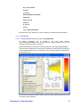
3.2.2.6.8
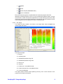
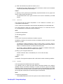
Q value with plots from 1-way ANOVA results (WINDOWS ONLY)
This script performs the exact same calculation as the previous script, but this script will
actually show four plots in the R Graphical User Interface as shown below
The plots can be used to determine an appropriate Q value cutoff and will give information
about the number of expected false positives.
3.2.2.6.9
Z-score Normalization
This script creates an experiment with Z-score normalization using all the samples of the
selected experiment.
Z-score = (ExprVal - Mean)
----------------------StDev
Input:
(1) Experiment: All samples in the Experiment will be sent to the external program
Knobs:
There are no parameters to be set for this script
Output:
(1) Experiment: A new experiment is presented to the user, with all the values normalized
with the Z score method, centered around 10
GeneSpring GX – R integration package
15
3.3
Post-installation modifications
There are a few modifications that may need to be performed, in order to ensure that the R
scripts can be executed successfully. For each of the supported platforms there are a few
possible changes and they are provided in the next sections.
3.3.1
WINDOWS
3.3.1.1
Change the location of the R program (OPTIONAL)
The script GS_exec_R.bat and GS_exec_R_GUI.bat assume that the R program is
installed in the GeneSpring GX data directory. This is where the full GeneSpring GX-R
integration package will install version 2.1.0 of the R program. If R was not installed in this
way and the user would like to use R stored in a different location, edit the GS_exec_R.bat
and GS_exec_R_GUI.bat scripts. These scripts are located in the data directory of the main
GeneSpring GX folder. When GeneSpring GX was installed in the default location the path
to the GS_exec_R.bat script would be:
C:\Program Files\SiliconGenetics\GeneSpring\data/GS_exec_R.bat
Change the following line to reflect the location of the R program:
rw2010\bin\Rterm.exe --no-restore --slave < %R_SCRIPT% > Rterm-output.txt
To something like
\YOUR\PATH\HERE\Rterm.exe --no-restore --slave < %R_SCRIPT% > Rterm-output.txt
The .bat file uses the program called Rterm.exe that is located in the bin directory of the
main R installation folder.
NOTE: When your R program is located in a directory that has a space in the name (Like
windows Program Files folder) you need to quote the directory name with double quotes.
For example, if R is installed in the default directory on Windows, the path to the Rterm.exe
program is:
C:\”Program Files”\R\rw2010\bin\Rterm.exe --no-restore --slave < %R_SCRIPT% >
Rterm-output.txt
Note the quotes around Program Files. Any folder that has a space in the name needs to
be quoted like this.
Also edit the GS_exec_R_GUI.bat script to reflect the different location of the R program.
Edit the line:
rw2010\bin\Rgui.exe --no-save --no-restore
to something like:
\YOUR\PATH\HERE\Rgui.exe --no-save --no-restore
(Remember to quote any folders with spaces in the name)
Note that the GS_exec_R_GUI.bat script uses a different R program, i.e. Rgui.exe and
there are no input or output files. This program will receive the R script in a different manner
as will be explained in other sections.
3.3.1.2
Non-default data directory location (OPTIONAL)
If the preference setting for the location of the GeneSpring GX data directory has been
changed in the past, you will need to move the .bat files, the R scripts and the rw2010
folder (If you chose to install the R program) to the original data directory in order for the
scripts to run successfully.
If you have changed your data directory settings, move the following files to the original data
directory:
GS_exec_R.bat
16
GeneSpring GX – R integration package
GS_exec-R_GUI.bat
boxplot.r
cv_filter.R
DifferentialExpression-LPE.R
gapFilter.R
power-anova.R
qvalue.R
Z_score.R
cat.exe
folder rw2010 (OPTIONAL)
Moving the files is only required if you have changed your GeneSpring GX data directory.
3.3.2
UNIX/MacOSX
3.3.2.1
Change the path to the GS_exec_R.sh script (REQUIRED)
By default, GeneSpring GX is installed in the user’s home directory
(~/SiliconGenetics/GeneSpring GX) and the External Program definitions have to be
changed to reflect the location of the scripts.
Edit the External Program definitions and change the path to the program GS_exec.R.sh.
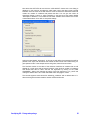
From the main GeneSpring GX window open the External Programs folder and select the
external program definition that you would like to edit, by selecting Inspect from the RIGHTCLICK pop-up menu.
From the External Program Inspector window, select the Edit Program Details button to edit
the external program definition.
GeneSpring GX – R integration package
17
Change the Command Line section. By default the path is:
/opt/SiliconGenetics/GeneSpring/data/GS_exec_R.sh
If GeneSpring GX is not located in the /opt directory, change the path accordingly. For
example, if your login name for UNIX is ‘peter’ and your home directory is in ‘/home/peter’,
and you installed GeneSpring GX with the default settings, you should change the path to
/home/peter/SiliconGenetics/GeneSpring/data/GS_exec_R.sh
Make the changes in all 7 external programs that are provided as examples.
18
GeneSpring GX – R integration package
3.3.2.2
Change the permissions of the GS_exec_R.sh script (REQUIRED)
Since the GS_exec_R.sh needs to be executed, the execute permissions need to be set for
the program, using the UNIX chmod command. The GS_exec_R.sh script is located in the
data directory of the main GeneSpring GX installation.
chmod a+x GS_exec_R.sh
This will ensure that the script can be executed by GeneSpring GX.
3.3.2.3
Change the location of the R program (OPTIONAL)
The script GS_exec_R.sh assumes that the R program is installed in a directory that is in
the user’s path. If the R program is not in the path, edit the path for the user or edit the
GS_exec_R.sh script. Change the following line to reflect the location of the R program:
R CMD BATCH --vanilla --slave < $Rscript
To something like
/YOUR/PATH/HERE/R CMD BATCH --vanilla --slave < $Rscript
3.3.2.4
Non-default data directory location (OPTIONAL)
If the preference setting for the location of the GeneSpring GX data directory has been
changed in the past, the scripts will not work. You will need to move the GS_exec_R.sh file
and the R scripts to the original data directory in order for the scripts to run successfully.
If you have changed your data directory settings, move the following files to the original data
directory:
GS_exec_R.sh
boxplot.R
cv_filter.R
DifferentialExpression-LPE.R
gapFilter.R
power-anova.R
qvalue.R
SAM.R
Z_score.R
Moving the files is only required if you have changed your GeneSpring GX data directory.
3.4
Creating External Programs using R
This section contains a description of the steps that need to be performed or installed to
allow GeneSpring GX to execute an R script. There are two version of this program, one for
MS Windows system “GS_exec_R.bat” and one for UNIX system called “GS_exec.R.sh” for
UNIX systems.
3.4.1
WINDOWS: GS_exec_R.bat
This Windows batch execution program GS_exec_R.bat is the main program that will be
used to execute the R code. This program will take any R script that contains the actual
code to be performed and instructs R to execute the program and to send the results back
to GeneSpring GX. There is usually no need to edit this script since it is a generic script that
can work with any proper R script, EXCEPT when R was not installed with the installer and
the user already has R installed in some different location. The contents of the .bat file is
explained below, and although it is not necessary to understand the working of the script, it
may be useful for future development efforts.
GeneSpring GX – R integration package
19
The contents of the batch script is presented below:
@echo off
set R_SCRIPT=%1
shift
:Loop
IF "%1" == "" GOTO Continue
set %1=%2
shift
shift
GOTO Loop
:Continue
cat.exe > GS_R_in.txt
rw2010\bin\Rterm.exe --no-restore --slave < %R_SCRIPT% > Rterm-output.txt
cat.exe < GS_R_out.txt
del GS_R_in.txt GS_R_out.txt Rterm-output
If you would wanted to use the .bat file on the Windows command line you would type
something like:
GS_exec_R.bat cv_filter.R CV_cutoff 100 Matching_conditions 1 < INPUT.txt >
OUTPUT.txt
This would execute the R script cv_filter.R located in the GeneSpring GX data directory
with the R program, using the parameter CV_cutoff set to 100 and the parameter
Matching_conditions set to 1.
3.4.1.1
GS_exec_R.bat file explained
A small explanation of each of the lines in the batch file is given below:
@echo off
This line instructs the script to not type the commands on the Standard Output since this
would interfere with the data parsing within GeneSpring GX later.
set R_SCRIPT=%1
This line saves the filename of the R script to be executed in the environment variable
R_SCRIPT.
shift
:Loop
IF "%1" == "" GOTO Continue
set %1=%2
shift
shift
GOTO Loop
:Continue
This set of lines assign the parameters that need to be passed to the R script. GeneSpring
GX will provide the script arguments and passes them on to the script GS_exec_R.bat as
command line parameters as key=value pairs. In this section the script loops through each
set of key=value pairs that are provided on the command line. If the script had two
arguments called ‘CV_cutoff’ and ‘Matching_conditions’ and the values set to be 100 and 3,
this will be converted into two environment variable of the same name with the value 100
and 3.
cat.exe > GS_R_in.txt
This line re-directs the output from GeneSpring GX (which could be the experiment data or
the selected gene list for instance) to a file called GS_R_in.txt using the program cat.exe
which is installed by the GeneSpring GX-R-Integration package installer. This GS_R_in.txt
file is a temporary file that will be used by the R script later. We re-direct the data from
GeneSpring GX into a file in the GeneSpring GX data directory, since it is somewhat easier
to deal with in R, but it is not absolutely necessary. We could elect to read the STDIN
stream directly in R.
The working directory for any of the external programs will be the GeneSpring GX data
directory,
which
on
WINDOWS
system
is
“C:\Program
Files\SiliconGenetics\GeneSpring\data”. If the location of the data directory has been
20
GeneSpring GX – R integration package
changed to a different location, the working directory WILL STILL BE THE OLD
DIRECTORY.
rw2010\bin\Rterm.exe --no-restore --slave < %R_SCRIPT% > Rterm-output.txt
This line will execute the R program and reads in the R script. The program we are using
from the R package is Rterm.exe which is the program that can execute R scripts without
the GUI interface. Later we will describe an example of using the Graphical User Interface to
R from GeneSpring GX. The Rterm program will execute the script that was the first
command line argument (Now saved into the environment variable R_SCRIPT) to the script.
The Rterm,exe program is located in the rw2010\bin directory in the GeneSpring GX data
directory and was installed there by the GeneSpring GX-R-Integration package installer (If
you elected to install R as part of the GeneSpring GX Integration package). The output from
the Rterm program is redirected to a temporary file in the GeneSpring GX data directory, to
ensure that any error message or warning from the R script will not interfere with the parsing
of the results by GeneSpring GX.
NOTE: If you DID NOT use the installer that included the R program and would like to use
your own version of R, change the path in this script accordingly.
cat.exe < GS_R_out.txt
This step re-directs the output of the R script that is written to a file, to the Standard Output
stream, so GeneSpring GX can pick up this stream and load the data into GeneSpring GX.
Most R scripts in the integration package will write the results of the analysis to a file called
GS_R_out.txt in the GeneSpring GX data directory and the cat.exe program is used again
to re-direct the output the STDOUT stream.
del GS_R_in.txt GS_R_out.txt Rterm-output
The last step is the clean-up stage and the temporary files are deleted using the Windows
del command.
3.4.1.2
Using the Graphical User Interface of R in GeneSpring GX
Except for command line version of R (Rcmd.exe), it is also possible to use the R Graphical
User Interface (Rgui.exe) to run R scripts. The GeneSpring GX R integration package can
also run any of the scripts in this interface and the integration package includes a special
.bat file that can be used to run any of the scripts in the GUI of R. Running scripts in the GUI
of R makes it possible to plot graphs and use any of the other GUI objects in R like the
graphical file browser (fileBrowser() for example).
3.4.1.3
GS_exec_R_GUI.bat
The .bat file that will execute an R script in the GUI of R is called “GS_exec_R_GUI.bat”
and the contents of the file with some short explanations is given below:
@echo off
copy %1 .Rprofile > copy-output.txt
shift
:Loop
IF "%1" == "" GOTO Continue
set %1=%2
shift
shift
GOTO Loop
:Continue
cat.exe > GS_R_in.txt
rw2010\bin\Rgui.exe --no-save --no-restore
cat.exe < GS_R_out.txt
del GS_R_in.txt GS_R_out.txt copy-output.txt .Rprofile
Most of the lines are similar to those in the non-GUI execution .bat file explained above with
the exception of the lines:
copy %1 .Rprofile > copy-output.txt
and
rw2010\bin\Rgui.exe --no-save --no-restore
GeneSpring GX – R integration package
21
Since it is not possible to execute a script with the GUI interface by providing the script on
the command line using the STDIN redirect “<”, the script to be executed is copied into a
special R file called “.Rprofile”. This file is automatically loaded and executed upon startup
of Rgui and this will ensure that our script is executed.
NOTE: The R script is copied into the file .Rprofile in the GeneSpring GX data directory and
any .Rprofile file that was already there will be overwritten. If your implementation requires
your own .Rprofile file, make appropriate changes to the script or moving your .Rprofile
changes to a site profile.
3.4.2
UNIX/Mac OS X: GS_exec_R.sh
The GS_exec_R.sh script that is provided on the UNIX systems R integration packages,
performs basically the same functionality as the GS_exec_R.bat script for Windows
described above. The script is given below:
#!/bin/bash
#Get the R script file name
Rscript=$1
shift
#Set the script parameters as environment variables
while [ $# -gt 0 ]
do
export $1
shift
done
#Take the output of GeneSpring and put it in a file for easier access
cat > GS_R_in.txt
#Run R (Let's hope it is in the path. If not edit this)
R CMD BATCH --vanilla --slave < $Rscript
#Put the results back into stdout
cat < GS_R_out.txt
#Clean up after ourselves
rm -f GS_R_out.txt GS_R_in.txt
The script takes the R script as the first command line argument and saves this into a
variable, after which it sets the External Program’s parameters as environment variables.
The script can take an unlimited number of parameters. The data from GeneSpring GX is
saved into a file, called “GS_R_in.txt” since it is a little easier to deal with the data in files,
that it is with data in the stdin stream.
NOTE: The R program is assumed to be in the command path of the user running the script.
If this is not guaranteed, edit the line to indicate the complete path to the R program as
described in section 3.3.2.3.
After running the actual script, the output is copied from a file onto the stdout stream and
the temporary files are cleaned up.
3.4.3
Create the R script
In this step you will write or install the R script that performs the actual function you would
like to integrate into GeneSpring GX. The R script should typically consist of three parts:
1) Read in the data and the parameters
2) Perform the analysis
3) Save the results in a file or the Standard Output stream
Most of the time, you would only need to have to worry about the second point, since we
have provided a suite of standard R functions that will perform some of the tedious but
important tasks of loading the data and parsing it out in data objects that can be
manipulated in R.
We have provided an R package called “GeneSpring” that is part of BioConductor version
1.4.0 and later and can be used to load and parse the data. See Appendix A for a
description of the “GeneSpring” R package.
22
GeneSpring GX – R integration package
For more information about writing R scripts refer to the User Manual for R at:
http://cran.r-project.org/manuals.html
The R scripts should be stored in the GeneSpring GX data directory, so they can be easily
referenced in the External Program definition.
3.4.4
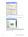
Create the External Program definition in GeneSpring GX
Once all the files are created and stored in their correct place, GeneSpring GX needs to be
instructed to be able to use the scripts and we will define them as external programs. To
configure GeneSpring GX to use the external programs, open GeneSpring GX and go to
the menu File->New External Program. This will open up a dialog box as displayed
below:
Name:
Start by giving the new External Program definition a name, like ‘Filter on CV’ (since we
will be using the example from Appendix B).
Folder
The external program can be placed in its own folder and you could either type the name
of a new or existing folder or select the folder from the navigator on the left.
Icon
If you want you can also assign an icon to the External Program, but in most cases leaving
this blank is fine. With the GeneSpring GX-R Integration package we have provided a
special icon that could be used for the R programs that you may write and the icon file is
called:
Rlogo16.gif
GeneSpring GX – R integration package
23
And you may choose this icon by pressing the Browse button and selecting the file, which
is located in the GeneSpring GX data directory.
Program Executable
GeneSpring GX supports three different types of External Programs. The proper External
Program or command line tool, A JAVA class or an HTTP call. In the case of executing an
R script we will leave the default setting “External Program”.
Command line:
In the command line text box we will type the following:
GS_exec_R.bat cv_filter.R
The first part is the R executing Batch program and the second part is the actual R script.
The second part could be any R script that you write and in this case we have used the
example R script “cv_filter.R”.
NOTE: On UNIX systems the complete path to the GS_exec_R.sh file needs to be given.
If GeneSpring GX was installed in the default location the command line should read:
/opt/SiliconGenetics/GeneSpring/data/GS_exec_R.sh cv_filter.R
Also note that, since the R scripts are stored in the same directory as the script, it is not
needed to provide the full path to the R script. If you choose to store your R scripts in a
different location than the R execution scripts, adjust the paths accordingly.
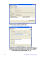
3.4.4.1
Input/Output/Delimiters/Arguments Tabs
The next section defines what the input (FOR the R script) and the output (FROM the R
script) is for the script. The INPUT tab defines what the R script will use as input and in the
case of the CV filter that would be the Experiment Condition Statistics.
Click on the INPUTS tab (if it is not already the default tab selected) and click on the <ADD
INPUT> button. A new dialog box is displayed. Choose Experiment Condition Statistics
from the left part of the dialog to choose this as the input for the R script.
When the Experiment Condition Statistics is selected, the right part of the dialog box
become active and here you can choose what data you would like to send to the R script.
Since the CV filter will be using the Average of the Normalized value and the Standard
Deviation of the Normalized values, select the checkbox next to the ‘Average’ and
‘Standard Deviation’ labels under the first column, which is called “Normalized Values” and
press OK.
24
GeneSpring GX – R integration package
Next select the OUTPUTS tab and click the <ADD OUPUT> button and a new dialog is
displayed. In this case we will select the radio button next to the label “Gene List With
Numbers” since the result of the filter will be a Gene List where the associated values will
contain the number of conditions that passed the filter. You can give the column of
Associated Values a name, by typing something in the text box at the bottom labeled
“Description of Numbers”. In this case we have used “Passed” as the label for the column
of associated values. Click <OK> to accept the settings.
Select the tabs labeled “Arguments”. In this tab we will define the arguments that will be
passed to the script, that will define what criteria the filter should use in determining if a
gene passes or fails. In the example we are using here, there will be two criteria.
The first filter criterion is the value of the minimum Coefficient of Variation that we will
tolerate for a given gene and the second criterion is the minimum number of conditions
that should have this CV value. Add the two arguments by clicking on the <ADD
ARGUMENT> button and changing the name of the first argument to “CV_cutoff” and
making the default value ‘100’. Press <RETURN> after changing the values.
The second argument name should be “Matching_conditions” with a default value of 1.
After the changes have been made the window should look like this:
GeneSpring GX – R integration package
25
There is no need to change the rest of the settings, so press <SAVE> to save the External
Program.
3.4.5
Running the External Program
The external program we have just created is stored in the External Programs section in
the Navigator window of GeneSpring GX:
In order to run the External Program you simply click the External Program’s name and the
script will be run. If you have defined any Arguments, a new dialog box will pop-up, asking
you to fill in the values for the Arguments. Since we have defined two arguments for the
CV filter program, a dialog box appear:
26
GeneSpring GX – R integration package
You can change the values if the default values are not appropriate and press <OK> to
start the actual script.
You will not see any activity except for the hourglass that indicates the filter is running. If
the filter is complete, a results window will appear and you will be able to save the results
in GeneSpring GX.
From this point the R script is successfully integrated into GeneSpring GX!
3.4.6
Using the Graphical User Interface for R
In the previous example we used the Rterm.exe program from the R package which will
execute the R script without providing any Graphical Interaction or feedback. It is possible
to use the Graphical User Interface for the R package, which will allow us to display any
plots or other graphical output that does not contain any data that can be stored in
GeneSpring GX.
In order to be able to use the GUI interface to R, the Rgui.exe program should be used in
stead of the Rterm.exe program to execute the R script. No other changes are needed and
we have provided an R execution BAT file to execute scripts that require a Graphical
Interface. The BAT file is called:
GS_exec_R_GUI.bat
Use this .bat file in stead of the standard GS_exec_R.bat file and the R script will be
executed in the Graphical environment of R.
GeneSpring GX – R integration package
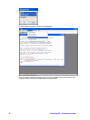
27
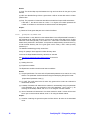
The provided External Program definition “Q value with plots” is an example of an R script
that is using the graphical environment of R in its execution. The definition of the External
Program is given below:
Note that the only difference with the definition for the External program “Q value” is the
fact that the “GS_exec_R_GUI.bat” file is used to execute the R script. Also note that the
R script used in both external programs is identical! The PLOT command in the “qvalue.R”
script is actually present in the NON-GUI version of the execution, but the plot is simply not
shown.
4
The GeneSpring R Package
The “GeneSpring” R package is part of the standard BioConductor offering and can be
installed with the standard mechanisms available in R and BioConductor. Only when you did
not install the complete R integration package would you require installing the “GeneSpring”
R library and a short description about the installation of the “GeneSpring” R package is
given below:
4.1
Installing the GeneSpring package
To install the “GeneSpring” R library, open the Graphical User interface for the R program.
28
GeneSpring GX – R integration package
From the menu Packages ensure that the BioConductor repository is activated, by choosing
“Select repositories” from the Packages menu.
A list of available repositories will be shown. Select the “Bioconductor” option and press OK.
GeneSpring GX – R integration package
29
Choose “Install packages(s)” from the Packages menu.
A list of available CRAN mirrors will appear. Choose the CRAN mirror that is closest to your
physical location to ensure the fastest response and press OK.
30
GeneSpring GX – R integration package
A list of available packages will appear. Select the package “GeneSpring” from the list and
press OK
GeneSpring GX – R integration package
31
The R program will download the package from the BioConductor website and install the
library files in the correct location. After the installation is complete, Press “y” to allow R to
delete the just downloaded file. It is safe to delete the downloaded files, since they have
been installed and are no longer needed. Deleting the files will save disk space.
32
GeneSpring GX – R integration package
For more information about
http://www.bioconductor.org/.
4.2
installing
packages
from
BioConductor
or
R
see
The GeneSpring functions
The GeneSpring package for R contains a number of functions and class definitions that
makes it easier to incorporate R scripts into GeneSpring GX. The functions will perform the
conversion of the specific GeneSpring GX format for Expression Experiments,
Interpretations and gene lists. The package will also provide functions for converting
GeneSpring GX objects into BioConductor objects like ‘exprSet’ and ‘phenoData’ objects for
example.
The name of the GeneSpring GX package is “GeneSpring”. Note the capitalization of the
word GeneSpring. At this point (R version 1.9.1) the capitalization is not strictly enforced,
but in the future it may be, so take care to refer to the package always in the correct
capitalization. Making the library active can be performed by using the command:
library(GeneSpring)
After the package has been installed. A list of functions and class definitions provided by the
GeneSpring package is given below and are described in more detail in the next section.
Functon name
Description
GSint()
Create GeneSpring Experiment Interpretation
object (class GSint)
Load GeneSpring Experiment Interpretation
from file and create Interpretation object
(class GSint)
Load GeneSpring Experiment Interpretation
from file and create BioConductor expression
object (class exprSet)
Load GeneSpring Experiment from file and
create Interpretation object (class GSint)
Load GeneSpring Experiment from file and
create BioConductor expression object (class
exprSet)
Load GeneSpring gene list from file
Save GeneSpring Experiment to file from
Interpretation object (class GSint)
Save GeneSpring gene list to file
Convert GeneSpring Interpretation object
GSload.int()
GSload.intBC()
GSload.exp()
GSload.expBC()
GSload.genelist()
GSsave.exp
GSsave.genelist()
GSint2BC()
GeneSpring GX – R integration package
33
(class GSint) to a BioConductor expression
object (exprSet)
Convert a BioConductor expression object
(exprSet) to a GeneSpring Interpretation
object (class GSint)
BC2GSint()
More information about the functions can also be obtained by using the help() or ? function
in R.
5
Appendix A. Complete R examples
This section contains the example scripts that are provided with the GeneSpring GX R
integration package. Read the comments for more information and on hints for writing your
own scripts.
5.1
Box plot
This script will take an Experiment Interpretation as create a Box plot in a graphic window.
No object is returned.
######################################################################################################
#
# boxplot.R
#
# Program that will accept an Interpretation and plot a Boxplot.
#
# Version 1.0.0
# Author: Thon de Boer, Agilent Technologies/SiliconGenetics, Redwood city, CA
# Last Update: 29-Nov-2004
#
# No environment variables defined
#
#
######################################################################################################
#
#Get the libraries that are needed
library(graphics)
library(stats)
library(utils)
library(Biobase)
library(GeneSpring)
#Load the Interpretation
i <- GSload.int()
#Plot the boxplot of the Normalized data on a logarithmic scale
boxplot(data.frame([email protected]),names=t(i@expparam[1,]),log ="y",notch=T,las=2,
main=paste(i@expName," (",i@ngenes," genes)",sep=""))
5.2
Filter on CV
This script will take an Experiment Interpretation as input and produce a Gene List as
output, of all the genes that pass the CV_cutoff and Matching_conditions settings.
######################################################################################################
#
# cv_filter.R
#
# Program that reads a GeneSpring Experiment Interpretation and creates a Gene List
# of those genes that fall within the parameters for the Coefficient of Variation
#
# Version 2.0.0
# Author: Thon de Boer, Agilent Technologies, Redwood city, CA
# Last Update: 17-Feb-2004
#
# Environment variable: CV_cutoff
; Value for the cutoff for the Coeficient of Variation
# Environment variable: Matching_conditions ; Number of conditons that need to pass
#
Can be ratio (less than 1) or
#
absolute number (> 1)
# Environment variable: Data_to_use
; Determines whether the CV should be calculated on the
#
Raw ("R" or "r") or the Normalized data ("N" or "n")
#
######################################################################################################
#Prepare GeneSpring environment
library(graphics)
library(stats)
library(utils)
34
GeneSpring GX – R integration package
library(GeneSpring)
#Read the Experiment Interpretation
gs.int<-GSload.int()
# Get the Parameters and do some sanity checking
Param <-Sys.getenv(c("CV_cutoff","Matching_conditions","Data_to_use"))
#Turn parameter into variables
CVcutoff <- if(Param[[1]] < 0) 0 else as.numeric(Param[[1]])
Nconditions <- if(Param[[2]] <= 0) 1 else as.numeric(Param[[2]])
firstLetter <- substr(toString(Param[[3]]),1,2)
DataToUse <- ifelse(((firstLetter == "r") || (firstLetter == "R")),"R",
ifelse(((firstLetter == "n") || (firstLetter == "N")),"N","R"))
#Create table of CV values using data described by DataToUse
# If the data is not there, we'll get into trouble, but we'll just return an empty genelist
CVvalues <- if(DataToUse == "N") 100*[email protected]/[email protected] else 100*[email protected]/[email protected]
#Make a table of all those values that pass the cutoff
# ... and check for those entries that don't have a SD value and have a NaN value
CVpass <- ifelse(is.na(CVvalues <= CVcutoff),FALSE,CVvalues <= CVcutoff)
#Make a list of those genes that pass the Nconditions setting
CVnumber <- apply(CVpass,1,sum)
CVok <- if(Nconditions >=1) CVnumber >= Nconditions else CVnumber/gs.int@numConditions >= Nconditions
genelist <- data.frame(genes = gs.int@genenames[as.logical(CVok)], pass = as.numeric(CVnumber[as.logical(CVok)]))
#Write the resulting Gene List
GSsave.genelist(genelist)
5.3
gapFilter
This script implements the BioConductor "gapFilter" genefilter.
######################################################################################################
#
# gapFilter.R
#
# This script implements the BioConductor "gapFilter" genefilter.
# The 'gapFilter' looks for genes that might usefully discriminate
# between two groups (possibly unknown at the time of filtering). To
# do this we look for a gap in the ordered expression values. The
# gap must come in the central portion (we exclude jumps in the
# initial 'Prop' values or the final 'Prop' values). Alternatively,
# if the IQR for the gene is large that will also pass our test and
# the gene will be selected.
#
# The script expects RAW data from an Interpretation to be sent from GeneSpring.
# Negative values and NA values will be removed before the filtering.
#
# Version 1.0.0
# Author: Thon de Boer, Agilent Technologies/SiliconGenetics, Redwood city, CA
# Last Update: 28-May-2004
#
# Environment variable: Gap: The size of the gap required to pass the test.
# Environment variable: IQR: The size of the Inter Quartile Range (IQR) required to pass the test.
# Environment variable: Prop: The proportion (or number) of samples to exclude at eitherend.
#
######################################################################################################
#Prepare GeneSpring environment
library(graphics)
library(stats)
library(utils)
library(GeneSpring)
library(Biobase)
library(genefilter)
#Read the Experiment Interpretation and Create BioConductor exprSet
gs.int<-GSload.int()
eSet <- GSint2BC(gs.int, what="raw")
# Get the Parameters and do some sanity checking
Param <-Sys.getenv(c("Gap","IQR","Prop"))
#Turn parameter into variables
Gap <- if(Param[[1]] < 0) 0 else as.numeric(Param[[1]])
IQR <- if(Param[[2]] < 0) 0 else as.numeric(Param[[2]])
Prop <- if(Param[[3]] < 1) 1 else as.numeric(Param[[3]])
#Create the filter function
Gfilter <- gapFilter(Gap, IQR, Prop)
ffun <- filterfun(Gfilter)
#Filter the genes
filteredEset <- genefilter(eSet, ffun)
GeneSpring GX – R integration package
35
#Create the gene list
genelist <- names(filteredEset[filteredEset])
#Write the resulting Gene List
GSsave.genelist(genelist)
5.4
DifferentialExpression-LPE
The program will calculate the P value for differential expression between the two groups,
using the Local Pooled Error Model as described by Jain et. al, Bioinformatics, Vol 19, 19451951 (2003)
######################################################################################################
#
# DifferentialExpression-LPE.R
#
# Program that will accept an experiment from GS and return a genelist with P values.
#
# The program will calculate the P value for differential expression between the two groups,
# using the Local Pooled Error Model as described by Jain et. al, Bioinformatics, Vol 19, 1945-1951 (2003)
# If the BH or BY multiple testing corrections are applied, the FDR is returned as the associated value.
# If the resampling method is used, the associated value represents the Z score for the gene.
#
# Version 2.0.0
# Author: Thon de Boer, Agilent Technologies, Redwood city, CA
# Last Update: 17-Feb-2005
#
# Environment variable: ExperimentParameter ; Name of the experimental parameter that define the groups
# Environment variable: Condition1
; Value of the eperimental parameter (Condition) defining group 1
# Environment variable: Condition2
; Value of the eperimental parameter (Condition) defining group 2
# Environment variable: PvalueCutoff
; P value cutoff value. Only genes with CORRECTED P values
#
below this value are returned.
# Environment variable: MulTestingCorrection ; Type of mutliple testing correction to use
#
#
######################################################################################################
#
#Get the libraries that are needed
library(graphics)
library(stats)
library(utils)
#Get the LPE library
library(LPE)
#Prepare GeneSpring environment
library(GeneSpring)
memory.limit(size = 2000)
#I had to re-implement the fdr.adjust function for the BH (or BY MTC), since the LPE version contains errors it seems
# It was ordering the matrix, but it lost the rownames.
my.fdr.adjust <- function (lpe.result, adjp = "BH")
{
if (adjp == "BH" || adjp == "BY") {
x.location <- grep("^x", names(lpe.result))
y.location <- grep("^y", names(lpe.result))
x <- lpe.result[, x.location]
y <- lpe.result[, y.location]
pnorm.diff <- pnorm(lpe.result$median.diff, mean = 0,
sd = lpe.result$pooled.std.dev)
p.out <- 2 * apply(cbind(pnorm.diff, 1 - pnorm.diff),
1, min)
p.adj <- mt.rawp2adjp(p.out, proc = adjp)
data.out <- data.frame(x = x, median.1 = lpe.result$median.1,
std.dev.1 = lpe.result$std.dev.1, y = y, median.2 = lpe.result$median.2,
std.dev.2 = lpe.result$std.dev.2, median.diff = lpe.result$median.diff,
pooled.std.dev = lpe.result$pooled.std.dev, abs.z.stats = abs(lpe.result$z.stats),
p.adj = p.adj)
return(data.out)
}
}
#======================================================================================
#Get environment variables
Param <-Sys.getenv(c("ExperimentParameter","Condition1","Condition2","PvalueCutoff","MulTestingCorrection"))
ExperimentParameter <- as.character(Param[1])
Condition1 <- as.character(Param[2])
Condition2 <- as.character(Param[3])
PvalueCutoff <- if(as.numeric(Param[4]) < 0) 0 else if(as.numeric(Param[4]) > 1) 1 else as.numeric(Param[4])
MulTestingCorrection <ifelse(is.na(grep(as.character(Param[5]),c("BH","BY","resamp","none","no"))[1]),"BH",as.character(Param[5]))
#Read the Experiment Interpretation
#The experiment
gs.int<-GSload.exp()
36
GeneSpring GX – R integration package
#Get rid of the missing values
[email protected] <- na.exclude([email protected])
#Add the parentheses and find it in the list of parameters, quit if we don't. No point doing anything if we don't know which
parameter to use
i <- charmatch(ExperimentParameter,row.names(gs.int@expparam))
if(is.na(i)) q()
#Preprocess the data. Normalize with dChip algorithm and LOWESS, set the threshold to a very small value, in case we get
pre-normalized data
expr <- preprocess([email protected],data.type = "dChip", LOWESS = TRUE, threshold = 1E-3)
#Find the data defining the two groups.
x <- expr[,gs.int@expparam[i,] == Condition1 ]
y <- expr[,gs.int@expparam[i,] == Condition2 ]
#Calcualte the baseline error distribution in 100 bins
x.var <- baseOlig.error(x, q=0.01)
y.var <- baseOlig.error(y, q=0.01)
#Do the LPE!
lpe.val <- lpe(x,y,x.var,y.var,probe.set.name=gs.int@genenames)
#Adjust the P value
#Could choose from c("BH", "BY","resamp","none","no")
#If it is no, we'll do it anyway, but send back the Raw p value
if(is.na(grep(MulTestingCorrection,c("BH","BY","resamp"))[1])) {
lpe.MTC <- my.fdr.adjust(lpe.val, adjp="BH")
} else if(MulTestingCorrection == "resamp") {
lpe.MTC <- fdr.adjust(lpe.val, adjp="resamp", target.fdr=PvalueCutoff)
} else {
lpe.MTC <- my.fdr.adjust(lpe.val, adjp=MulTestingCorrection)
}
#Create the gene lists
if(MulTestingCorrection == "resamp") {
geneindex <- lpe.val[,"z.stats"]>=lpe.MTC[1,"z.critical"]
genelist <- data.frame(genes=row.names(lpe.val)[geneindex], Z.stats=lpe.val[geneindex,"z.stats"])
} else {
#Get the column name
column <paste("p.adj.adjp.",ifelse(is.na(grep(MulTestingCorrection,c("BH","BY"))[1]),"rawp",MulTestingCorrection),sep="")
#Create the GeneList
geneindex <- lpe.MTC[,column] <= PvalueCutoff
genelist <- data.frame(genes=row.names(lpe.MTC)[geneindex],FDR = lpe.MTC[geneindex,column])
}
# Write the resulting Gene List
GSsave.genelist(genelist)
5.5
DifferentialExpression-SAM
he program will calculate the d value for differential expression between the two groups,
using the SAM (Significance Analysis of Microarrays) method, implemented in R, as
described by Tusher, V.G., Tibshirani, R., and Chu, G. (2001). Significance analysis of
microarrays applied to the ionizing radiation response, _PNAS_, 98, 5116-5121.
NOTE: A LICENSE IS REQUIRED FOR COMMERCIAL USE OF SAM. Non-commercial
use is permitted. For more information on how to obtain a license for commercial use of
SAM see http://otl.stanford.edu/industry/resources/sam.html
######################################################################################################
#
# SAM.R
#
# Program that will accept an experiment from GS and return a genelist with d values.
#
# The program will calculate the d value for differential expression between the two groups,
# using the SAM method as described by Tusher, V.G., Tibshirani, R., and Chu, G. (2001).
# Significance analysis of microarrays applied to the ionizing radiation response, _PNAS_, 98, 5116-5121.
#
# Version 2.0.0
# Author: Thon de Boer, Agilent Technologies, Redwood city, CA
# Last Update: 18-Feb-2005
#
# Environment variable: ExperimentParameter ; Name of the experimental parameter that define the groups
# Environment variable: Condition1
; Value of the eperimental parameter (Condition) defining group 1
# Environment variable: Condition2
; Value of the eperimental parameter (Condition) defining group 2
# Environment variable: Q_cutoff
; Q value cutoff.
#
#
GeneSpring GX – R integration package
37
######################################################################################################
#
#Get the libraries that are needed
library(graphics)
library(stats)
library(utils)
library(siggenes)
library(GeneSpring)
memory.limit(size = 2000)
#Get environment variables
Param <-Sys.getenv(c("ExperimentParameter","Condition1","Condition2","Q_cutoff"))
ExperimentParameter <- as.character(Param[1])
Condition1 <- as.character(Param[2])
Condition2 <- as.character(Param[3])
Q_cutoff <- if(as.numeric(Param[4]) < 0) 0 else if(as.numeric(Param[4]) > 1) 1 else as.numeric(Param[4])
#Get the GeneSprint Experiment
gs.int<-GSload.exp()
#Add the parentheses and find it in the list of parameters, quit if we don't.No point doing anything if we don't know which
parameter to use
i <- charmatch(ExperimentParameter,row.names(gs.int@expparam))
if(is.na(i)) q()
#Get the id's for the group and create a sub matrix of only the two group
#Get the two groups as separate sets and combine them again
x <- log2([email protected][,gs.int@expparam[i,] == Condition1 ])
x.cl <- rep(0,dim(x)[2])
y <- log2([email protected][,gs.int@expparam[i,] == Condition2 ])
y.cl <- rep(1,dim(y)[2])
gs <- data.frame(x=x,y=y)
gs.cl <- c(x.cl,y.cl)
#Perform the SAM with the default settings
sam.out <- sam(gs,gs.cl, gene.names=gs.int@genenames)
#Create a delta plot if we run this script interactive
if(interactive()) {
delta.plot(sam.out)
}
#Get the genes that show a Q value less than the Q_cutoff and return the d values
geneindex <- [email protected] < Q_cutoff
#Create the GeneList
genelist <- data.frame(genes = names(sam.out@d)[geneindex], delta = sam.out@d[geneindex])
# Write the resulting Gene List
GSsave.genelist(genelist)
5.6
Power of ANOVA
This script will calculate the power of a gene, using the variance within and between group
of replicates.
######################################################################################################
#
# power-anova.R
#
# Program that accepts a GeneSpring Experiment interpretation,
# and calculates the power.anova for each gene
#
# Version 2.0.1
# Author: Thon de Boer, Agilent Technologies, Redwood city, CA
# Last Update: 23-Mar-2005
#
# Environment variable: SignificanceRequired ; The desired significance for the power calculation
#
######################################################################################################
#Prepare GeneSpring environment
library(graphics)
library(stats)
library(utils)
library(GeneSpring)
# Read the Experiment Interpretation
gs.int<-GSload.int()
# Get the Parameters and do some sanity checking
Param <-Sys.getenv(c("SignificanceRequired"))
SignificanceRequired <- if(Param[[1]] < 0) 0 else if(Param[[1]] > 1) 1 else as.numeric(Param[[1]])
#Create list of Variances BETWEEN the groups
#Take the variances of all the means of the groups (Column 1 of exp)
VarBetween <- apply([email protected],1,var)
38
GeneSpring GX – R integration package
#Create list of Variances WITHIN the groups
#Take the median of all the SD data columns and convert it to variances (Column 2 of exp)
VarWithin <- apply([email protected],1,median)^2
#Create a list of the number of replicates for each gene
#Take the median of all the numbers of replicates (Column 3
numReps <- apply([email protected],1,median)
of exp)
#Calculate the power for each gene
powerValues<-power.anova.test(groups=c(gs.int@numConditions),n=numReps[numReps > 0],between.var=VarBetween[numReps >
0],within.var=VarWithin[numReps > 0],sig.level=SignificanceRequired,power=NULL)
#Create the two genelists
genelist <- data.frame(genes=gs.int@genenames[numReps > 0],power = as.numeric(powerValues$power))
#Write the resulting Gene List
GSsave.genelist(genelist)
5.7
Q value with plots
This is a complete example of an R script.
This program will take an as input, a list of P values and calculate a list of Q values and filter
the Q values based on the provided Qvalue_cutoff. The program will also produce four
plots, allowing the user to determine appropriate Q value cutoff values.
######################################################################################################
#
# qvalue.R
#
# Program that reads a GeneSpring gene list with P values as associated values,
# and returns a gene list with Q values as associated values that pass the cutoff
#
# Version 1.1.1
# Author: Thon de Boer, Agilent Technologies/SiliconGenetics, Redwood city, CA
# Last Update: 24-Jun-2004
#
# Environment variable: Q_cutoff
; Value for the cutoff of the Q value
# Environment variable: bootsrap
; Indicates if the bootstrap method should be used.
#
Possible values: "yes" (= bootstrap", "no" (= smoother)
# Environment variable: robust
; Indicates whether it is desirable to make the estimate more robust
#
Possible values: "yes", "no" (Default)
#
######################################################################################################
library(graphics)
library(stats)
library(utils)
#####
#
# Original code by Storey starts here
#
#Version 1.1; Updated June 2003
#These functions estimate the q-values for a given set of p-values. The
#statistical methodology mainly comes from:
#Storey JD. (2002) A direct approach to false discovery rates.
#Journal of the Royal Statistical Society, Series B, 64: 479-498.
#See http://faculty.washington.edu/~jstorey/qvalue/ for more info.
#All functions were written by John D. Storey. Copyright 2002,2003 by John D. Storey.
#All rights are reserved and no responsibility is assumed for mistakes in or caused by
#the program.
qvalue <- function(p, lambda=seq(0,0.95,0.05), pi0.meth="smoother", fdr.level=NULL, robust=F) {
#Input
#=============================================================================
#p: a vector of p-values (only necessary input)
#fdr.level: a level at which to control the FDR (optional)
#lambda: the value of the tuning parameter to estimate pi0 (optional)
#pi0.method: either "smoother" or "bootstrap"; the method for automatically
#
choosing tuning parameter in the estimation of pi0, the proportion
#
of true null hypotheses
#robust: an indicator of whether it is desired to make the estimate more robust
#
for small p-values and a direct finite sample estimate of pFDR (optional)
#
#Output
#=============================================================================
#call: gives the function call
#pi0: an estimate of the proportion of null p-values
#qvalues: a vector of the estimated q-values (the main quantity of interest)
#pvalues: a vector of the original p-values
#significant: if fdr.level is specified, and indicator of whether the q-value
#
fell below fdr.level (taking all such q-values to be significant controls
#
FDR at level fdr.level)
GeneSpring GX – R integration package
39
#This is just some pre-processing
if(min(p)<0 || max(p)>1) {
print("ERROR: p-values not in valid range"); return(0)
}
if(length(lambda)>1 && length(lambda)<4) {
print("ERROR: If length of lambda greater than 1, you need at least 4 values."); return(0)
}
m <- length(p)
#These next few functions are the various ways to estimate pi0
if(length(lambda)==1) {
pi0 <- mean(p >= lambda)/(1-lambda)
pi0 <- min(pi0,1)
}
else{
pi0 <- rep(0,length(lambda))
for(i in 1:length(lambda)) {
pi0[i] <- mean(p >= lambda[i])/(1-lambda[i])
}
if(pi0.meth=="smoother") {
spi0 <- smooth.spline(lambda,pi0,df=3)
pi0 <- predict(spi0,x=max(lambda))$y
pi0 <- min(pi0,1)
}
if(pi0.meth=="bootstrap") {
minpi0 <- min(pi0)
mse <- rep(0,length(lambda))
pi0.boot <- rep(0,length(lambda))
for(i in 1:100) {
p.boot <- sample(p,size=m,replace=T)
for(i in 1:length(lambda)) {
pi0.boot[i] <- mean(p.boot>lambda[i])/(1-lambda[i])
}
mse <- mse + (pi0.boot-minpi0)^2
}
pi0 <- min(pi0[mse==min(mse)])
pi0 <- min(pi0,1)
}
}
if(pi0 <= 0) {
print("ERROR: The estimated pi0 <= 0. Check that you have valid p-values or use another lambda.meth."); return(0)
}
#The estimated q-values calculated here
u <- order(p)
v <- rank(p)
qvalue <- pi0*m*p/v
if(robust) {
qvalue <- pi0*m*p/(v*(1-(1-p)^m))
}
qvalue[u[m]] <- min(qvalue[u[m]],1)
for(i in (m-1):1) {
qvalue[u[i]] <- min(qvalue[u[i]],qvalue[u[i+1]],1)
}
#The results are returned
if(!is.null(fdr.level)) {
retval <- list(call=match.call(), pi0=pi0, qvalues=qvalue, pvalues=p, significant=(qvalue <= fdr.level),
lambda=lambda)
}
else {
retval <- list(call=match.call(), pi0=pi0, qvalues=qvalue, pvalues=p, lambda=lambda)
}
class(retval) <- "qvalue"
return(retval)
}
qplot <- function(qobj, rng=0.1) {
#Input
#=============================================================================
#qobj: a q-value object returned by the qvalue function
#rng: the range of q-values to be plotted (optional)
#
#Output
#=============================================================================
#Four plots:
#Upper-left: pi0.hat(lambda) versus lambda with a smoother
#Upper-right: q-values versus p-values
#Lower-left: number of significant tests per each q-value cut-off
#Lower-right: number of expected false positives versus number of significant tests
q2 <- qobj$qval[order(qobj$pval)]
if(min(q2) > rng) {rng <- quantile(q2, 0.1)}
p2 <- qobj$pval[order(qobj$pval)]
par(mfrow=c(2,2))
lambda <- qobj$lambda
if(length(lambda)==1) {lambda <- seq(0,max(0.95,lambda),0.05)}
pi0 <- rep(0,length(lambda))
for(i in 1:length(lambda)) {
pi0[i] <- mean(p2>lambda[i])/(1-lambda[i])
}
spi0 <- smooth.spline(lambda,pi0,df=3)
40
GeneSpring GX – R integration package
pi00 <- round(qobj$pi0,3)
plot(lambda,pi0,xlab=expression(lambda),ylab=expression(hat(pi)[0](lambda)),pch=".")
mtext(substitute(hat(pi)[0] == that, list(that= pi00)))
lines(spi0)
plot(p2[q2<=rng],q2[q2<=rng],type="l",xlab="p-value",ylab="q-value")
plot(q2[q2<=rng],1:sum(q2<=rng),type="l",xlab="q-value cut-off",ylab="significant tests")
plot(1:sum(q2<=rng),q2[q2<=rng]*(1:sum(q2<=rng)),type="l",xlab="significant tests",ylab="expected false positives")
par(mfrow=c(1,1))
}
qwrite <- function(qobj, filename="my-qvalue-results.txt") {
#Input
#=============================================================================
#qobj: a q-value object returned by the qvalue function
#filename: the name of the file where the results are written
#
#Output
#=============================================================================
#A file sent to "filename" with the following:
#First row: the function call used to produce the estimates
#Second row: the estimate of the proportion of false positives, pi0
#Third row and below: the p-values (1st column) and the estimated q-values (2nd column)
cat(c("Function call:", deparse(qobj$call), "\n"), file=filename, append=F)
cat(c("Estimate of the overall proportion of false positives pi0:", qobj$pi0, "\n"), file=filename, append=T)
for(i in 1:length(qobj$qval)) {
cat(c(qobj$pval[i], qobj$qval[i], "\n"), file=filename, append=T)
}
}
#####
#
# Original code by Storey stops here
#
#Prepare GeneSpring environment
library(GeneSpring)
# Get the Parameters and do some sanity checking
Param<-Sys.getenv(c("Q_cutoff","bootstrap","robust"))
Qcutoff <- if(Param[[1]]>1) 1 else if(Param[[1]]<0) 0 else as.numeric(Param[[1]])
bootstrap <- if(Param[[2]] != "no") "bootstrap" else "smoother"
robust <- if(Param[[3]] != "no") TRUE else FALSE
#Getting the data
g.list <- GSload.genelist()
qobj <- qvalue(g.list[,2], fdr.level=Qcutoff, pi0.meth=bootstrap, robust=robust)
genelist <- data.frame(genes = g.list[qobj$significant,1], qvalue = qobj$qvalues[qobj$significant])
#Save the gene list
GSsave.genelist(genelist)
#Make the plots if we are in an interactive session
if (interactive()) qplot(qobj)
5.8
Z score normalization
This script will normalize an experiment using the Z score method.
######################################################################################################
#
# Z_score.R
#
# Program that reads a GeneSpring Experiment,
# and returns a new GeneSpring experiment with this data again normalized using the Z score method.
#
# Version 2.0.0
# Author: Thon de Boer, Agilent Technologies/SiliconGenetics, Redwood city, CA
# Last Update: 29-Apr-2005
#
######################################################################################################
#
#Prepare GeneSpring environment
library(graphics)
library(stats)
library(utils)
library(GeneSpring)
#Read the Experiment
gs.int<-GSload.exp()
#Z score function definition
zscore <- function(l){
#This function takes a list and returns the Z score for each of the members of the list
# The mean and SDev are calculated over the members of the list
# Input: list of numbers
# Outout: list of dim(list) with the Z score for each of the members
GeneSpring GX – R integration package
41
s<-sd(l,na.rm=TRUE)
m<-mean(l,na.rm=TRUE)
return((l-m)/s)
} #####End of Z score function definition
#Calculate the Z scores
a.nor.new <- t(apply([email protected],1,zscore))
#Make a new GeneSpring experiment with just the Z score data
# We could not try to convert the COntrol values to retain the original RAW values
# since GeneSpring cannot deal with negative Control values
# The experiment name gets suffixed with "Z score" and the parameters are copied
newGSint <- GSint(a.nor=a.nor.new, expName=paste(gs.int@expName,"Z score"), expparam=gs.int@expparam,
genenames=gs.int@genenames)
# Save the experiment
GSsave.exp(newGSint)
42
GeneSpring GX – R integration package