1
Institutionen för systemteknik
Department of Electrical Engineering
Examensarbete
Pilot Study of Systems to Drive Autonomous
Vehicles on Test Tracks
Examensarbete i Reglerteknik utfört
vid Tekniska högskolan i Linköping
av
Erik Agardt
Markus Löfgren
LITH-ISY-EX--08/4042--SE
Linköping 2008
Department of Electrical Engineering
Linköpings universitet
SE-581 83 Linköping, Sweden
Linköpings tekniska högskola
Linköpings universitet
581 83 Linköping
Pilot Study of Systems to Drive Autonomous
Vehicles on Test Tracks
Examensarbete i Reglerteknik utfört
vid Tekniska högskolan i Linköping
av
Erik Agardt
Markus Löfgren
LITH-ISY-EX--08/4042--SE
Handledare:
Christian Lundquist
isy, Linköpings universitet
Göran Åhling
EDAC/Volvo 3P
Göran Åhlin
Volvo 3P
Examinator:
Thomas Schön
isy, Linköpings universitet
Linköping, 28 March, 2008
Avdelning, Institution
Division, Department
Datum
Date
Division of Automatic Control
Department of Electrical Engineering
Linköpings universitet
SE-581 83 Linköping, Sweden
Språk
Language
Rapporttyp
Report category
ISBN
Svenska/Swedish
Licentiatavhandling
ISRN
Engelska/English
Examensarbete
C-uppsats
D-uppsats
Övrig rapport
2008-03-28
—
LITH-ISY-EX--08/4042--SE
Serietitel och serienummer ISSN
Title of series, numbering
—
URL för elektronisk version
http://www.control.isy.liu.se
http://www.ep.liu.se
Titel
Title
Förstudie av System för Körning av Autonoma Fordon på Provbanor
Pilot Study of Systems to Drive Autonomous Vehicles on Test Tracks
Författare Erik Agardt, Markus Löfgren
Author
Sammanfattning
Abstract
This Master’s thesis is a pilot study that investigates different systems to drive autonomous and non-autonomous vehicles simultaneously on test tracks. The thesis
includes studies of communication, positioning, collision avoidance, and techniques
for surveillance of vehicles which are suitable for implementation. The investigation results in a suggested system outline.
Differential GPS combined with laser scanner vision is used for vehicle state
estimation (position, heading, velocity, etc.). The state information is transmitted
with IEEE 802.11 to all surrounding vehicles and surveillance center. With this
information a Kalman prediction of the future position for all vehicles can be
estimated and used for collision avoidance.
Nyckelord
Keywords
Autonomous vehicles, GPS, DGPS, WLAN, fast handover, IEEE 802.11, laser
scanner, lidar, collision avoidance, Kalman filter
Abstract
This Master’s thesis is a pilot study that investigates different systems to drive autonomous and non-autonomous vehicles simultaneously on test tracks. The thesis
includes studies of communication, positioning, collision avoidance, and techniques
for surveillance of vehicles which are suitable for implementation. The investigation results in a suggested system outline.
Differential GPS combined with laser scanner vision is used for vehicle state
estimation (position, heading, velocity, etc.). The state information is transmitted
with IEEE 802.11 to all surrounding vehicles and surveillance center. With this
information a Kalman prediction of the future position for all vehicles can be
estimated and used for collision avoidance.
v
Acknowledgments
We would first of all thank our supervisors at AB Volvo, Göran Åhlin and Göran
Åhling. These two persons have been of great importance for the performance of
this master thesis and have always encouraged and helped us during the time.
We would also thank Per-Olov Fryk who initiated this project, our examiner
Thomas Schön, and our supervisor at the university, Christian Lundquist.
Finally we would thank all of the employees at Volvo 3P who have helped us
and made our work a great time.
Erik Agardt and Markus Löfgren
Göteborg, January 2008
vii
Contents
1 Introduction
1.1 Background . . . . . .
1.2 Volvo 3P . . . . . . . .
1.3 Problem Specification
1.4 Limitations . . . . . .
1.5 Thesis Outline . . . .
.
.
.
.
.
.
.
.
.
.
.
.
.
.
.
.
.
.
.
.
.
.
.
.
.
.
.
.
.
.
.
.
.
.
.
.
.
.
.
.
.
.
.
.
.
.
.
.
.
.
.
.
.
.
.
.
.
.
.
.
.
.
.
.
.
.
.
.
.
.
.
.
.
.
.
.
.
.
.
.
.
.
.
.
.
.
.
.
.
.
.
.
.
.
.
.
.
.
.
.
1
1
1
1
3
3
2 Position System
2.1 Satellite Navigation . . . . . . . .
2.1.1 Global Positioning System
2.1.2 Differential GPS . . . . .
2.1.3 Carrier-Phase, L1\L2 . .
2.2 Inertial Navigation System . . .
2.3 Combined DGPS/INS System . .
2.4 Vision System . . . . . . . . . . .
2.4.1 Line Following Systems .
2.4.2 Camera Systems . . . . .
2.4.3 Radar Sensors . . . . . .
2.4.4 Laserscanners . . . . . . .
2.5 Complete Position System . . . .
.
.
.
.
.
.
.
.
.
.
.
.
.
.
.
.
.
.
.
.
.
.
.
.
.
.
.
.
.
.
.
.
.
.
.
.
.
.
.
.
.
.
.
.
.
.
.
.
.
.
.
.
.
.
.
.
.
.
.
.
.
.
.
.
.
.
.
.
.
.
.
.
.
.
.
.
.
.
.
.
.
.
.
.
.
.
.
.
.
.
.
.
.
.
.
.
.
.
.
.
.
.
.
.
.
.
.
.
.
.
.
.
.
.
.
.
.
.
.
.
.
.
.
.
.
.
.
.
.
.
.
.
.
.
.
.
.
.
.
.
.
.
.
.
.
.
.
.
.
.
.
.
.
.
.
.
.
.
.
.
.
.
.
.
.
.
.
.
.
.
.
.
.
.
.
.
.
.
.
.
.
.
.
.
.
.
.
.
.
.
.
.
.
.
.
.
.
.
.
.
.
.
.
.
.
.
.
.
.
.
.
.
.
.
.
.
.
.
.
.
.
.
.
.
.
.
.
.
5
5
5
6
8
8
8
9
11
11
11
12
17
3 Communication Systems
3.1 STDMA . . . . . . . . . . . . . . . . . . .
3.1.1 VDL Mode 4 . . . . . . . . . . . .
3.1.2 TACSYS/CAPTS . . . . . . . . .
3.1.3 STDMA Summary . . . . . . . . .
3.2 Wireless Local Area Network . . . . . . .
3.2.1 IEEE 802.11 . . . . . . . . . . . .
3.2.2 WLAN With Dual Antennas . . .
3.2.3 Selective Channel Scanning . . . .
3.2.4 Handover Using Neighbour Graph
3.2.5 IEEE 802.11 Summary . . . . . . .
3.2.6 ZigBee . . . . . . . . . . . . . . . .
3.2.7 WiMax . . . . . . . . . . . . . . .
.
.
.
.
.
.
.
.
.
.
.
.
.
.
.
.
.
.
.
.
.
.
.
.
.
.
.
.
.
.
.
.
.
.
.
.
.
.
.
.
.
.
.
.
.
.
.
.
.
.
.
.
.
.
.
.
.
.
.
.
.
.
.
.
.
.
.
.
.
.
.
.
.
.
.
.
.
.
.
.
.
.
.
.
.
.
.
.
.
.
.
.
.
.
.
.
.
.
.
.
.
.
.
.
.
.
.
.
.
.
.
.
.
.
.
.
.
.
.
.
.
.
.
.
.
.
.
.
.
.
.
.
.
.
.
.
.
.
.
.
.
.
.
.
.
.
.
.
.
.
.
.
.
.
.
.
.
.
.
.
.
.
.
.
.
.
.
.
19
19
19
20
20
20
20
21
22
22
25
25
26
.
.
.
.
.
.
.
.
.
.
.
.
.
.
.
.
.
.
.
.
.
.
.
.
.
ix
x
Contents
4 Collision Avoidance
4.1 Collision Avoidance Prediction . . . . . . . . . . . . . . . . . . . .
4.2 Vehicle States Message . . . . . . . . . . . . . . . . . . . . . . . . .
4.3 Collision Avoidance Vision . . . . . . . . . . . . . . . . . . . . . . .
27
28
37
38
5 Measurements and Data Collection
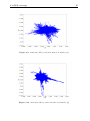
5.1 GPS coverage . . . . . . . . . . . . . .
5.1.1 Static GPS Coverage Hällered .
5.1.2 Test Track GPS Coverage . . .
5.1.3 GPS Accuracy . . . . . . . . .
5.1.4 Dual GPS . . . . . . . . . . . .
5.1.5 Differential GPS . . . . . . . .
5.2 Laser Scanner Data Collection . . . .
5.3 WLAN coverage . . . . . . . . . . . .
5.3.1 WLAN range . . . . . . . . . .
.
.
.
.
.
.
.
.
.
.
.
.
.
.
.
.
.
.
.
.
.
.
.
.
.
.
.
.
.
.
.
.
.
.
.
.
.
.
.
.
.
.
.
.
.
.
.
.
.
.
.
.
.
.
.
.
.
.
.
.
.
.
.
.
.
.
.
.
.
.
.
.
.
.
.
.
.
.
.
.
.
.
.
.
.
.
.
.
.
.
.
.
.
.
.
.
.
.
.
.
.
.
.
.
.
.
.
.
.
.
.
.
.
.
.
.
.
.
.
.
.
.
.
.
.
.
.
.
.
.
.
.
.
.
.
.
.
.
.
.
.
.
.
.
41
41
41
42
44
48
48
53
54
54
6 Conclusions
6.1 Positioning Conclusions . . . . . .
6.1.1 Positioning . . . . . . . . .
6.1.2 Vision . . . . . . . . . . . .
6.2 Communication Conclusions . . . .
6.2.1 WLAN . . . . . . . . . . .
6.3 Survaillence Conclusions . . . . . .
6.4 Collision Avoidance Conclusions . .
6.5 System Movability Conclusions . .
6.6 Future Work . . . . . . . . . . . .
6.6.1 Positioning System . . . . .
6.6.2 Lidar System . . . . . . . .
6.6.3 Communication System . .
6.6.4 Collision Avoidance System
6.6.5 Fault Detection . . . . . . .
.
.
.
.
.
.
.
.
.
.
.
.
.
.
.
.
.
.
.
.
.
.
.
.
.
.
.
.
.
.
.
.
.
.
.
.
.
.
.
.
.
.
.
.
.
.
.
.
.
.
.
.
.
.
.
.
.
.
.
.
.
.
.
.
.
.
.
.
.
.
.
.
.
.
.
.
.
.
.
.
.
.
.
.
.
.
.
.
.
.
.
.
.
.
.
.
.
.
.
.
.
.
.
.
.
.
.
.
.
.
.
.
.
.
.
.
.
.
.
.
.
.
.
.
.
.
.
.
.
.
.
.
.
.
.
.
.
.
.
.
.
.
.
.
.
.
.
.
.
.
.
.
.
.
.
.
.
.
.
.
.
.
.
.
.
.
.
.
.
.
.
.
.
.
.
.
.
.
.
.
.
.
.
.
.
.
.
.
.
.
.
.
.
.
.
.
.
.
.
.
.
.
.
.
.
.
.
.
.
.
.
.
.
.
.
.
.
.
.
.
.
.
.
.
57
57
57
58
58
58
59
59
59
59
59
60
60
60
60
.
.
.
.
.
.
.
.
.
.
.
.
.
.
.
.
.
.
.
.
.
.
.
.
.
.
.
.
Bibliography
61
A Satellite Navigation
A.1 History . . . . . . . . . . . . . . . . . . . . . . . . . . . . . . . . .
A.2 GPS . . . . . . . . . . . . . . . . . . . . . . . . . . . . . . . . . . .
67
67
67
B Inertial Navigation Systems
B.1 Dead Reckoning . . . . . . . . . . . . . . . . . . . . . . . . . . . . .
73
73
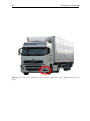
C Prototype Systems
C.1 PATH . . . . . . . . . .
C.2 VW Golf GTi 53+1 . . .
C.3 Team LUX . . . . . . .
C.4 Previous Volvo projects
C.4.1 LKAB . . . . . .
76
76
76
77
77
77
.
.
.
.
.
.
.
.
.
.
.
.
.
.
.
.
.
.
.
.
.
.
.
.
.
.
.
.
.
.
.
.
.
.
.
.
.
.
.
.
.
.
.
.
.
.
.
.
.
.
.
.
.
.
.
.
.
.
.
.
.
.
.
.
.
.
.
.
.
.
.
.
.
.
.
.
.
.
.
.
.
.
.
.
.
.
.
.
.
.
.
.
.
.
.
.
.
.
.
.
.
.
.
.
.
.
.
.
.
.
.
.
.
.
.
.
.
.
.
.
Contents
xi
C.4.2 VTEC Prototype truck . . . . . . . . . . . . . . . . . . . .
77
D Mathematics
D.1 Haversine Equation . . . . . . . . . . . . . . . . . . . . . . . . . . .
D.2 Covariance . . . . . . . . . . . . . . . . . . . . . . . . . . . . . . .
79
79
79
E Kalman filter
E.1 Extended Kalman filter . . . . . . . . . . . . . . . . . . . . . . . .
80
80
F Globalsat
82
G Oxford Tech RT 3002
87
H Oxford Tech RT-Base
90
I
93
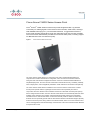
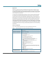
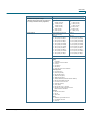
Cisco Aironet 1240G Series Access Point
J Antenna Specifications
100
Chapter 1
Introduction
1.1
Background
This master thesis has its background at Volvo’s test track at Hällered. On the test
track an endurance circuit is built with the purpose to expose the vehicles tested
to general wear and tear. The drivers are exposed to very hard working conditions
primarily because of heavy vibrations when driving repeatedly numbers of laps on
the endurance track. Long time exposure to these conditions is not suitable for the
human physique. The drivers’ working environment would benefit from a decrease
of the exposure to vibrations. In order to obtain as much measurement data as
possible without causing the driver harm, the idea to investigate the possibility to
drive vehicles autonomously. With an autonomous vehicle, it is possible to repeat
the path on the track with a higher precision than a human driver can achieve.
There were several questions to be answered, such as: Is this project possible?
Which techniques should then be used? Which modifications should be done at
Hällered? To answer these questions, Volvo initiated this as a master thesis project
for two master students. The result is a pilot study that are investigating if the
theory of autonomous driving is possible and if so an investigation of what kind
of equipment would be needed to implement this idea.
1.2
Volvo 3P
This master thesis has been performed at Volvo 3P. Volvo 3P is a business unit
within AB Volvo that works with Volvo Trucks, Mack Trucks, Renault Trucks and
BA Asia. 3P stands for Product Planning, Purchasing, Product Development and
Product Range Management for the companies within AB Volvo.
1.3
Problem Specification
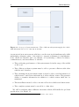
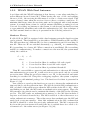
The primary goal of this thesis work is to investigate the possibilities of autonomous operation of vehicles. The aim is to design a system allowing several au1
2
Introduction
Figure 1.1. A proposed system structure. Three different subsystems supply the vehicle
with information needed to run autonomously.
tonomous and non-autonomous vehicles to use the test track simultaneously while
maintaining adequate safety. Our task is to suggest techniques for implementations, which are suitable and cost efficient, for positioning, collision avoidance,
communication, and surveillance of vehicles.
• The positioning performance of the system must be in the range of the width
of the road.
• The collision avoidance system must be able to prevent collisions with other
vehicles and obstacles.
• The communication performance must at least be able to send information of
vehicle states1 and receive information of other vehicles’ states. The system’s
ability to transfer information in addition to vehicle status shall also be
estimated.
• The surveillance must be able to monitor all active vehicles and their states.
• The complete system must be movable to other sites.
We will be studying three different structures which will handle the problem
specification. See Figure 1.1.
1 Vehicle
states include position, velocity and status of the vehicle
1.4 Limitations
1.4
3
Limitations
In this thesis, the data collection is limited to Göteborg, Hällered, and nearby
areas. For that reason the moveability and the system performance at other test
tracks cannot be evaluated in this thesis. The hardware tested is limited to equipment available at AB Volvo. The system designed may consist of other parts, which
have not been validated. This thesis will not include control of an autonomous
vehicle.
1.5
Thesis Outline
In the following chapters we will investigate the different sub-systems and present
the techniques for these.
Chapter 2 describes different navigation systems and navigation tools to be used
in our application.
Chapter 3 compares the different communication techniques that have been investigated and describes the theoretical background.
Chapter 4 describes the principles and techniques which are used to prevent
collisions between autonomous vehicles, non-autonomous vehicles, and other objects.
Chapter 5 presents the data that has been collected for this project.
Chapter 6 summarizes the thesis. This chapter also includes suggestions for
future work to expand this project.
Chapter 2
Position System
To obtain a position of a vehicle several different techniques can be used. This
chapter will introduce the techniques which have been investigated. The major
problem of the positioning is the accuracy. The systems considered in this chapter
are positioning by satellite navigation, vision units, and dead reckoning.
2.1
Satellite Navigation
Positioning by satellite navigation is nowadays a very common feature. The most
used system is the NAVSTAR Global Positioning System (henceforth referred as
GPS in this thesis).
2.1.1
Global Positioning System
The basic function of satellite navigation and GPS function is described in Appendix A. Many vehicles nowadays can have a GPS wayfinder integrated within
the vehicle. This is often a typical commercially available GPS receiver1 unit with
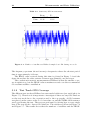
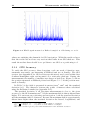
an update frequency of 1 Hz and with a standard deviation accuracy2 of 15 m.
This accuracy is too low to fulfill the demands of keeping a vehicle within one
lane of the road. To obtain the demands of the positioning system the standard
deviation needs to be less than 1 m [1]. Even the update frequency of the position
in a typical GPS is too low (see Example 2.1). A GPS unit with a higher update
frequency and with a standard deviation accuracy of 15 m has an accuracy which
is too imprecise. Our conclusion is that the typical GPS not qualifies to be a part
of the positioning system.
1 The phrase typical GPS receiver is referring to the Garmin GPS 35/36 that is used as a
standard component within Volvo trucks [1]
2 The positioning standard deviation, 95% of the time
5
6
Position System
Example 2.1: 1 Hz GPS example
If the GPS update frequency is 1 Hz and the test vehicle is traveling at 15 m/s
(54 km/h). The vehicle will advance 15 m between measurement positions. This
can be a serious problem in for instance cornering manoeuvres. To obtain the
wanted resolution (in meters) the GPS update frequency can be estimated by the
following equation.
V elocity[m/s]
F requency[Hz] =
(2.1)
Resolution[m]
2.1.2
Differential GPS
A differential GPS is an enhancement to the standard GPS system. It operates
by a stationary ground network or by fixed ground local stations. By knowing the
exact position of the stationary receiver, it can calculate the errors from satellite
signals and send out the differential corrections to the vehicle. A base station
covers a small area and the differential correction is a local correction. There
are several different techniques that are currently in use to obtain the differential
correction signals. The two most common techniques are Wide Area Correction
System (WACS) and Local Area Correction System (LACS) [48].
EGNOS/WAAS
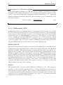
European Geostationary Navigation Overlay Service (EGNOS) is a Satellite Based
Augmentation System (SBAS) that is under development in Europe. The EGNOS
system is a WACS. The system started operations in July 2005, and will be certified for use in 2008. The North American Wide Area Augmentation System
(WAAS) is similar but has no European coverage [21]. EGNOS uses three geostationary satellites which send out a ranging signal (similar to ordinary GPS signal).
EGNOS also uses a network of ground stations that calculates the errors (clock,
ionospheric disturbances, etc.) and sends out a correction signal (see Figure 2.1).
This correction increases the accuracy of the GPS to approximately 2 m [19]. The
problem with this system is that the accuracy is not good enough to keep the
vehicle within one lane of the roadway.
SwePos
The Swedish GPS correction service EPOS is available for use. The service is
provided by the Swedish company SwePos. It uses the FM-radio frequency to
send out the correction signals. The coverage of this technique is very good for
use in Sweden but the update frequency is between between 3 and 5 seconds. The
accuracy is good, but the update frequency is too slow [57]. For that reason this
technique is not suitable for this project.
2.1 Satellite Navigation
7
Figure 2.1. Wide Area Correction System (WACS). Two GPS satellites (1 and 2) with
stationary reference stations (3 and 4) that supplies the user with position information
and correction signals to obtain a high accuracy position [50].
SwePos also offers a Network Real-Time Kinematic correction. This is based
on a subscription provided by the GSM network. This provides with centimeter
accuracy but the correction service is expensive and every user needs a subscription
[57]. This technique is not suitable to our demands due to the subscription cost.
OmniSTAR
The OmniSTAR is a GPS system which offers GPS correction which can improve
the accuracy of the GPS receiver. The OmniSTAR concept is a subscription
service to their GPS receiver. The subscription supplies the customer with access
to the correction signal of their satellites. It works like a WACS system, where
multiple OmniSTAR GPS reference sites calculate the error of the signal. By
sending up correction signals to the satellites from the American and Australian
Network Control Center the correction data is received and applied in real-time.
The system is available with an accuracy below 10 cm with the OmniSTAR service
subscription [45]. This technique provides great accuracy but is still dependent on
a subscription service for every user and because of this service it is not suitible
for this prodject.
Local Area DGPS
One option to get differential correction signals is to use a separate DGPS base
station. The range of the base station is limited, and the position accuracy decreases with increasing distance to the base station. The base station is stationary
and sends out correction signals to the DGPS receiver with e.g. a radio modem.
With the local area correction signals the DGPS receiver obtains great accuracy.
A position accuracy below 50 cm is achievable with this technique. The local area
8
Position System
DGPS system is fairly expensive to implement, but it is free from any subscription services and is very suitable for implementation within a restricted area. The
cost of implementing a local DGPS system is according to given indications, in
the same range as one single year of subscription fees for eight units using e.g.
Omnistar services. The local DGPS system is not limited to a number of users
and it offers a high grade of accuracy [48]. This technique is very suitable to our
demands and will be further investigated.
2.1.3
Carrier-Phase, L1\L2
A typical GPS receiver calculates its position by the data that is sent from the
GPS satellites. A second form of precise monitoring is called Carrier-Phase (CP)
Enhancement. In order to obtain greater accuracy such a GPS receiver uses the CP
from the satellite signal. The CP approach utilizes the L1 carrier wave3 , which has
a period a thousand times smaller than the bit period of the Coarse/Acquisition
code (C/A), as an additional clock signal in order to reduce the uncertainty. The
phase difference error in the normal GPS results in a position error within 2 to
3 meters. Using the CP method, this position error could, in the ideal case,
reach 3 cm resolution4 . Realistic use of a CP-GPS (L1) coupled with differential
correction, Carrier Phase DGPS (CDGPS), gives a normal position accuracy of
approximatly 50 centimeters. If this technique is expanded with a L1\L2 receiver,
the accuracy is at centimeter level (see appendix A.2). An accuracy comparision
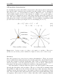
is presented in Figure 2.2 and Table 2.1 [48, 42]. To keep the vehicle within the
roadway, a CDGPS would be recommended.
2.2
Inertial Navigation System
An inertial navigation system is a completely independent system5 . The positioning is based on integration of the small changes in direction and velocity. This is
detected by an Inertial Measurement Unit (IMU). Due to the minor offset in the
change of the position, the new calculated position can quickly drift to a great error. See Figure 2.3 for a schematic drawing of an inertial navigator. This system
is not suitable for use as a stand alone system due to the increasing error, but
the technique can be used as a complement to increase the total accuracy of the
combined systems [28, 48].
2.3
Combined DGPS/INS System
To obtain greater accuracy than the DGPS provides, several systems use a combination of a DGPS unit and an IMU. To increase the position accuracy between
DGPS samples inertial gyros and/or accelerometers are used to calculate the new
3 See
Appendix A.2 for carrier wave information.
performance is valid for kinematic measuring. Static measuring obtains even better
accuracies.
5 See Appendix B for more information.
4 The
2.4 Vision System
9
Figure 2.2. Summary of expected differential GPS concepts and position accuracies
[48].
position. Due to the DGPS combination, the system will not suffer from severe
drifting in the calculation of the new position. After every new DGPS sample, the
inertial system has a known position to calculate from. This technique can deliver
position with a very high sample rate (e.g. 250 Hz [39]). When adding a Kalman
filter to this setup, the system obtains even greater resolution. The Kalman filter
uses the input errors to give the system an even more exact position. The standard deviation is below 2 cm in some products6 . To further improve the position
accuracy a single/double antenna GPS, differential GPS correction, and an IMU
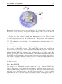
unit can be used. See Figure 2.4 for a block diagram of DGPS/INS unit. The
input to the figure is the measured value of the gyros and accelerators [47, 48].
The ordinary use of this technique in the automotive industry is to measure
vehicle handling (roll-, pitch-, yaw-angles7 , slip, etc) [47]. A combined DGPS/INS
system would be an appropriate choice for this application, but this technique
leads to very expensive hardware.
2.4
Vision System
This section presents different vision systems that are used for automotive implementation such as collision avoidance, adaptive cruise control, and lane detection
systems. Vision systems can be used for positioning with reference points by
measuring distance and heading to the reference points.
6 See
7 See
Appendix G for example.
Figure B.1
10
Position System
Figure 2.3. A schematic drawing of a Inertial Navigation System (INS). The system
contains gyros and accelerometers to obtain information in three dimensions and a computional unit to process the information signals.
Figure 2.4. Schematic block diagram of a combined DGPS and INS unit. The computional unit combines the information from the GPS receiver (single or dual antenna),
the INS system, and receives differential correction signals from a differential base station via the radio modem. All this information supplies the user with a high accuracy in
position [47].
2.4 Vision System
11
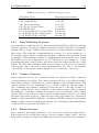
Table 2.1. Accuracy of different navigation types
Navigation Type
GPS
GPS with EGNOS
GPS L1 Carrier Phase
GPS L1\L2 Carrier Phase
OmniSTAR GPS
Local Area DGPS L1 Carrier Phase
Local DGPS L1\L2 Carrier Phase
Local DGPS L1\L2 with INS
2.4.1
Theoretical performance
≈15 m [1]
≈2 m [19]
1.8 m [42]
1.5 m [42]
sub m [42]
0.45 m [42]
sub dm [42]
sub dm [47]
Line Following Systems
A system that is commonly used by Automated Guided Vehicles (AGVs) is the line
following principle. By using a guidance system the vehicle can follow a predefined
guidance line by itself. Vehicles with monotonous driving schedules are suited for
this system. The principle of implementation is usage of a vision system (e.g. a
laser scanner) that detects a significant marking or reflection material and uses it
as guidance. This technique can also be implemented with magnetic force, which
the PATH project (see Appendix C.1) in California is one example of. Using
permanent magnets in the roadway and detectors in the vehicle results in a robust
system. However this technique suffer from problems as relocation and mobility
of the system, due to the need of static implementation [49]. Due to our demands
of movability of the system, this technique is not of interest to our needs.
2.4.2
Camera Systems
Camera systems can use one or several cameras in combination with a computer
to perform image processing. The camera systems can give a very high resolution,
and advanced target classification is possible thanks to the detailed images. The
camera systems are very dependent on good light conditions and free sight of
view. Darkness and weather conditions as rain and snow, lower the resolution of
the images which leeds to lower reliability of the camera system. When combined
with infrared, or thermal, cameras the system can see in the dark. Such camera
systems suffer from reflection of heat radiation which makes it hard to use within
navigation and safety purposes. The image processing algorithms are computation
intensive which may make it difficult to maintain reliability when the environment
changes rapidly (such as at high speed driving) [31]. Advantages and disadvantages
of this system are presented in Table 2.2.
2.4.3
Radar Sensors
Radio detection and ranging (Radar) is one of the most common tracking sensors.
It has been used for automotive purposes, such as adaptive cruise control. A radar
emits electro-magnetic radiation to illuminate targets. It uses the same antenna to
12
Position System
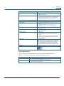
Table 2.2. Camera system [31]
Advantages
Cost efficient system
High resolution
Advanced target classification
Disadvantages
Sensitivity to light conditions
Sensitivity to dirt and weather
High computational demands
Table 2.3. Radar system [31]
Advantages
Bad-weather performance
Automotive usage
Range
Disadvantages
Bad resolution
Clutter
Ghost and multipath reflections
emit as to receive, by switching between sending and receiving mode. It sends out a
conical lobe that is reflected by the object. To obtain information about the target,
the system receives an echo of the emitted signal and can calculate the distance to
the target. One sensor can do a mechanical sweep, or electronically switches can
be used to alternate between different sensors, each located at different emission
angles. These techniques make it possible to survey a wider area. In general for
automotive purposes the field of view is 10◦ -15◦ . For short distances (less than
200m), the radar has good performance in bad-weather conditions, e.g. darkness,
rain, haze, and snow. Although good performance, the resolution to verify the
objects’ identities is not very good due to the wide lobe. For this project, the
radar needs assistance of other devices to obtain acceptable performance. The
radar suffers from unwanted reflections called clutter. Reflections from the road
surface might give "ghost" obstacles. Multipath propagation might also occur. The
precision of the radar is not suitable as a stand alone implementation of navigation.
The best use of this application would be as an Automatic Cruise Control (ACC)
system [31]. Advantages and disadvantages of this system are presented in Table
2.3.
2.4.4
Laserscanners
The laser scanner (also known as Lidar) works like a radar. A laser pulse with a
defined duration is sent and reflected by an object. The reflection of the object
is captured by a photo diode and transformed into signals in an optoelectronic
circuit. The time interval between the pulse of light being sent and its reflection
being received indicates the distance to the object which reflected the light. In
addition to the radar, the laser pulse is quite narrow. This gives the laser scanner
a higher resolution of the object.
By rotating a mirror, the laser range finder operates as a scanner and the mirror
deflects each outgoing beam. The mirror’s continuous rotation, in conjunction
with the pulsing laser, generates a complete environmental profile of the vehicle
2.4 Vision System
13
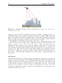
within the laser scanners visible range (see Figure 2.5). The laser scanning system
has been adapted by several autonomous prototype vehicles. The lidar technique
has also been implemented by Volvo Technology at their Volvo Integrated Safety
Truck (see Appendix C.4.2). Usage of the lidar is for example collision avoidance,
pedestrian safety, blind spot surveillance [31].
Lidar Performance
The laser scanner has a very high sample rate. This makes it suitable for scanning
the environment at high speeds. This technique is similar to millimeter-radar
(mm-radar), but is a less expensive technique to use. The range and the narrow
lobe of the laser makes the system very precise. It provides a high resolution of
the pixel map and could give more detailed information than the mm-radar. The
laser scanner system is also very tolerant to clutter. Again, the narrow beam does
not suffer from reflections of nearby objects in the same degree as a radar [31].
The intensity of the reflected laser pulse can be detected by the lidar and can
easily be projected into a gray scale picture. This is very useful to implement in the
lane detection feature (see Figure 2.6). The laser scanner is relatively insensitive
to the surrounding light conditions [31, 35, 58, 54].
Despite all of these advantages, the laser scanner suffers from a couple of weaknesses. In the automotive industry, most of these systems are at prototype stage.
This makes the price high at this stage, but will probably drop when prototypes go
to large series production. In similarity with the camera system the laser scanner
must have a free line of sight. Rain and fog could also interfere with the correct
echo detection. A single pulse can be reflected by rain or other weather obstacles.
Due to the technique of reflection the lidar has difficulties to detect dark and rough
objects. These objects are hard to detect due to absorbation of the laser beam.
The lens also needs to have a clear view to avoid false detections [31, 43].
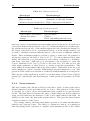
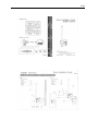
Figure 2.5. An exploded view of a laserscanner. The laser beam is reflected on to a
rotating mirror to spread the view of sight. The echo of the laser beam is received and
the distance and the heading can be calculated [26].
14
Position System
Figure 2.6. Animation of the principle of lane detection using a laserscanner [26]
Lidar Technique
The lidar vision system uses several different techniques to increase its performance. Dirt on the lens could result in a false detection. The dirt reflections can
to a certain extent be filtered by processing the signal. This applies to limited
surface elements. The obstacles of the lidar, such as bad weather performance is
improved by using four-echo technology. An object, such as a raindrop or another
vehicle, would normally generate one reflection or echo per laser pulse. By increasing the number of echoes to as many as four per pulse, and by filtering the echoes
and removing the false echoes, the lidar has significantly optimized and refined
object detection [26]. For implementation at a truck that is supposed to drive
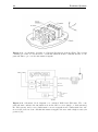
under very rough road conditions, the system is exposed to hard oscillation. The
system handles this problem with a multilayer technique (see Figure 2.7). The
laser beam is split into four different layers and the distance measurements are
taken independently for each of these layers with an aperture angle of 3.2◦ . This
allows compensation for pitching of the vehicle, caused by an uneven surface or
driving manoeuvres such as braking and accelerating. Since the beam, generated
by each laser pulse, is split into four layers, the lidar sensors can evaluate the data
from the reflections (up to 16 reflections per measurement, four echoes and four
layers). This technique gives a high grade resolution and reliability [24].
All products are in a prototype stadium. A truck implementation is available
as well as the possibility to produce products according to customer specifications.
The scan of the surrounding environment detects objects, due to the many reflection points, in a high resolution picture. This also results in that the detected
object can be identified by its significant structure. The detected objects can be
assigned with an ID number, a velocity, and a heading. Due to the high scanning
frequency a high resolution model of the surrounding environment can be estimated. In the model can objects be classified as a car, a truck, a pedestrian, a
fixed object, etc. By using the heading and distances to known objects, navigation
2.4 Vision System
15
Figure 2.7. Example of a multilayer lidar. The lidar beam is spread in different angles
to obtain additional information of the surroundings.
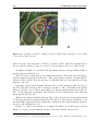
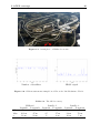
Figure 2.8. Lidar object detection. The picture to the left shows the lidar echoes of the
surrounding environment corresponding to the right picture.
is possible. In Figure 2.8 the different cars’ velocity and headings are marked with
circles and arrows. The fixed object is marked with a square. In the picture to
the left, it is shown how the lidar detects objects and different contours in the surrounding environment. The precision of the position can also be increased when
using precise high level maps [62]. Detection of the lanemarkings can also be used
for road navigation and vehicle control [13, 35, 37].
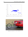
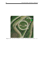
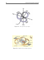
An installation of two laser scanners in the front of the truck will give a satisfying visual coverage to prevent collisions and the ability to navigate by nearby
objects (see Figure 2.9). The lidar function and performance is suitable as a vision
system to an autonomous system. The lidar system is used for safety applications by many developing companies and is frequently used by the D.A.R.P.A8
autonomous vehicles [6, 26]. Advantages and disadvantages of the system is presented in Table 2.4.
8 The D.A.R.P.A (Defense Advanced Research Projects Agency) is the central research and
development organization for the U.S. Department of Defense (DoD)[7].
16
Position System
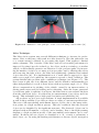
Figure 2.9. Field of vision of a laser scanner mounted on the right front of a truck. By
using this location, the scanner covers approximatly 270◦ of view [26].
Table 2.4. Lidar system [31]
Advantages
Resolution
Minimal clutter
Light insensitive
Photo detection
Used in automotive application
Disadvantages
Dirt sensitivity
Weather sensitivity
Prototype stadium
2.5 Complete Position System
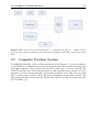
17
Figure 2.10. An extended system structure to run autonomously. To obtain accurate
position, the position system uses information from DGPS, CAN/INS, and from a vision
unit.
2.5
Complete Position System
To fulfill the demands of the problem specification in Chapter 1.3, the performance
of the CDGPS is of interest as a positioning system and will be further investigated.
The input signals to the position system will in this stage be from a DGPS, the
CAN (Controller Area Network) information, and from the vision system. A block
diagram over the system principle is presented in Figure 2.10. The vision system
that, at this point, seems to have the most advantages is the lidar system. By
integrating the lidar vision with the DGPS, the vehicle’s position system increases
its robustness [25].
Chapter 3
Communication Systems
The complete system is depending on a communication system in order to implement interacting between vehicles. To surveil the traffic of the test track the
communication system will be used to upload and download information about
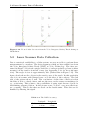
the vehicles states. In this chapter several techniques will be presented and investigated as to the possibillity to obtain the wanted performance.
3.1
STDMA
STDMA stands for Self organizing Time Division Multiple Access. This method
was developed by Håkan Lans and is used for positioning and identification of
aircrafts (VDL Mode 4) and ships (AIS). The STDMA data link is divided into a
number of time slots to send data messages. It is self organized and the communicator can by itself find a free slot and send the message to the free slot. Every
node must have access to global time and the regular transmissions are sent as
"heartbeats". This means that different types of data can be sent on the data link,
using just one frequency. All communicators within radio distance will be able to
hear the message. The STDMA scheme ensures that access is free of collisions and
that the bandwidth per node is guaranteed [18, 23, 33].
3.1.1
VDL Mode 4
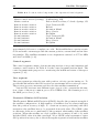
VDL Mode 4 (Very high frequency Data Link Mode 4) is the standard of the International Civil Aviation Organization (ICAO). The main purpose for VDL Mode 4
is to send an Automatic Dependent Surveillance Broadcast (ADS-B) signal to complement the ground radar and the surveillance service. The technique is also used
as a Flight Information Service Broadcast (FIS-B). It sends the aircraft’s position
and identification to all surrounding aircrafts. It can also send complementary
information, such as weather information, from the control tower to the aircraft.
The data link transmits digital data in a standard 25 kHz VHF communication
channel [2, 18, 23, 33].
19
20
Communication Systems
The problem with this is that the total bandwidth is limited due to the number
of slots that can be used. This results in a limited number of users and/or a small
amount of data that can be sent [2, 18, 23, 33].
3.1.2
TACSYS/CAPTS
The Taxi and Control System/Cooperative Area Precision Tracking System (TACSYS/CAPTS) is an innovation project from Fraport AG. The general function of
this system is to increase the accuracy of airport ground navigation in poor weather
conditions. It uses the signals from the on-board transponders. By measuring the
time of the incoming transponder signals the distance to the object can be calculated by triangulation. The transponder signal includes an ID-tag so the identity
of the vehicle also can be determined [4].
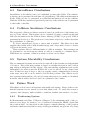
3.1.3
STDMA Summary
The STDMA technique, e.g. VDL-Mode 4, is a very robust and reliable communication system. It has been approved by the aeronautical industry, which shows
out its reliability. Because of the system’s limitations in transfer rate and in the
number of vehicles that can simultaneously use it, this system is not interesting for
our application. The future expansion possibilities would also be narrowed down
and the possibility to send larger amounts of data would be limited.
3.2
3.2.1
Wireless Local Area Network
IEEE 802.11
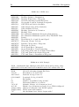
IEEE 802.11x is the standard of Wireless Local Area Network (WLAN). The IEEE
802.11 is followed by an index letter (a,b,g,n1 in this case) which indicates what
version of WLAN it is. In table 3.1 the capacity and performance of different
802.11-protocols is presented. This is the most common communication technique
adapted for wireless data transfer.
Table 3.1. IEEE 802.11x specifications of frequency and transfer rate
Protocol
802.11a
802.11b
802.11g
802.11n
1 802.11n
is a draft version.
Operation Freq.
5 GHz
2.4-2.5 GHz
2.4-2.5 GHz
2.4 and/or 5 GHz
Transfer Rate
54 Mbit
11Mbit
54 Mbit
248 Mbit
3.2 Wireless Local Area Network
3.2.2
21
WLAN With Dual Antennas
A problem with the WLAN-technique is that latency occurs when switching between different Access Points (AP). When leaving the area of APi and entering
the area of APj , the receiving module must do a scan to obtain a new signal. This
causes a latency time when the receiver does not have a wireless connection. To
minimize this latency time, the receiving unit can be equipped with a dual antenna
system. A normal latency time for a single antenna (including roaming) is about
1 second. By adding one antenna to the system, it can decrease the handover time
to approximately 60 milliseconds with fast authentication [44]. One technique of
the dual antenna handover theory is presented in the following subsection.
Handover Theory
If a Mobil Node (MN) is equipped with a dual antenna system the handover time
can be reduced. The system has to work with two WLAN InterFaces (IF1 and IF2 ).
The MN uses these two different IF’s for data communication and for searching for
new AP. These two IF are switched alternately, e.g. when IF1 is communicating,
IF2 is searching for a better AP. When connection is established, IF1 is searching
and IF2 is communicating. To make a connection to the next AP, the system must
satisfy the condition:
Pc − Pp
where
Pc
Pp
Pt
>
Pt
= Power level in dBm of candidate AP radio signal
= Power level in dBm of used AP radio signal
= Power level in dBm of predefined threshold
Then IF2 can establish a connection and authentication to the next AP. During
this authentication processes, IF1 is still active in a receive-mode only for a certain
protection time. When the protection time is over, IF1 is disconnected and starts
searching for another AP. Using this overlapping sequence, the system completes
the handover with minimal package loss. The handover flowchart is presented in
Figure 3.1 [44].
One solution to speed up the handover process is to shorten the authentication
time and the location registration time. The Mobile Switch (MS) authenticates a
MN on behalf of the radius server when the MN switches from APi to APj . After
establishing an air link, the MN sends an authentication start request. Then, the
MS generates a key that is used to maintain the identity of the MN for the following
process. The MN sends an authentication message to the MS that includes a
response word derived from the key. The MS forwards it to the radius server as a
radius authentication message. The radius server then authenticates the MN and
sends back a response message. After this authentication the MS confirms that
the MN is identical to what was previously authenticated. The MS compares the
key from the previous transaction and if the key is verified there is no need to do
a transaction to the radius server (see Figure 3.2) [44].
22
Communication Systems
Figure 3.1. Flowchart of the handover process using dual antenna technique. This
schematic flow describes how the system switches between the two network interfaces
[44].
3.2.3
Selective Channel Scanning
The IEEE 802.11b/g works with several different channel frequency distributions.
In Sweden the channel distribution is according to Figure 3.3 and the distribution
is divided to 14 possible channels, but several of these are overlapping. Among
these channels only three of them are not overlapping, and together they cover
the entire bandwidth. These channels are 1, 6 and 11. To reduce the scanning
time and decrease the handover time it is possible to use a selective scanning
procedure. It takes less time to scan three channels instead of fourteen. This is
called a selective scan [53].
3.2.4
Handover Using Neighbour Graph
To make a faster handover it is possible to use a technique that builds and sends
out a Neighbour Graph (NG). A NG is an undirected graph where each edge
represents a mobility path between two AP’s [40, 41].
Definition 3.1 (Neighbour Graph)
G
V
e
N (APi )
=
=
=
=
(V, E)
{{vi : vi } = (APi , channel) ∈ {AP1 , AP2 , . . . , APi }}
(APi , APj )
{APik : APik ∈ V, (APi , APik ) ∈ E}
3.2 Wireless Local Area Network
23
Figure 3.2. Fast authentication when switching between two APs. The flowchart describes how the authentication requests and responses are handled.
Figure 3.3. Channel frequency distribution in IEEE 802.11b [53]
24
Communication Systems
Figure 3.4. (a) Map of an AP’s example positions. (b) Neighbour graph corresponding
to the AP’s position in (a).
where G is the data structure of NG, V consists of AP’s and their channels, E is
the set which consists of edge (e), and N is the neighbor AP’s of a AP [40, 41].
A simple example of a possible AP placement and its corresponding neighbor
graph is shown in Figure 3.4.
The NG can be generated by two different methods. The first uses the reassociation request from the mobile node. The reassociation request contains MAC2
address of the old AP. The second way to build the NG is to use the Move-Notify
message3 [36, 40].
Both the reassociation request and the Move-Notify message adds an edge to
the NG. The first mobile node to change from APi to APj will suffer from a high
latency, but the cost of this is amortized over all upcoming changes from APi to
APj . If the network is restarted the NG-info can be loaded from a file with the
latest known NG [40, 41].
When no mobile node hand-offs from APi to APj is done in a given time interval
T , the edge should be removed from the NG [40, 41]. The major advantage of an
automatically generated NG is adaption to changes in the AP placement, physical
topology, AP malfunction, etc.
Figure 3.5 shows an example of a simple flowchart of an NG server and in
Figure 3.5 b the corresponding flowchart of the NG client is shown [36].
2 Media
3 An
Access Control
Inter AP Protocol (IAPP) message that are used to reduce link layer handoff latency [38]
3.2 Wireless Local Area Network
a
NG server
25
b
NG client
Figure 3.5. Flowchart of the NG server and NG client.
3.2.5
IEEE 802.11 Summary
The IEEE 802.11 technique offers "off the shelf technology". This is a very common
technique used both by professionals and by the general public. The widespread
popularity of these products makes the price low and the accessibility high, which
is a major advantage of this products. It is a widespread technique and with
increasing performance. Adoption of this technique for automotive use (fore example roadside systems) points to an effective range of 150 m in radius [46]. This
features makes the IEEE 802.11 technique very interesting as a communication
tool. The problem is the limited range of the system.
3.2.6
ZigBee
ZigBee is a high level communication protocol which is based on the IEEE 802.15.4
standard. It is a low-power radio based solution for wireless personal area networks
(WPANs). The advantages of the ZigBee is low power consumption, giving a long
26
Communication Systems
life battery, and secure networking. The disadvantage are on the other hand that
the data rate is low and the product is not approved as a standard [8]. This
technique is not suitable to use as a communication device due to the low data
rate.
3.2.7
WiMax
Worldwide Interoperability for Microwave Access (WiMax) is the standard IEEE
802.16. The use of WiMax is to cover large areas with wireless access, approximately 70 Mbit/second over 500 km. It operates between the 2.5 GHz and the 5.8
GHz frequency band. The main purpose of this system is to provide the final user
with a wireless connection without cable connection. In Sweden it operates in the
licensed frequency band of 3.5 Ghz. This has to be licensed from the Post- och
telestyrelsen (PTS) [64]. This technique supports a great range but is not intended
for implementation as a closed network in a small area. The implementation is
not cost efficient and the interface would be difficult to implement. This makes
the technique not suitable for our needs.
Chapter 4
Collision Avoidance
Collision avoidance is a common aspect in the automotive industry nowadays.
The preventative work is to reduce the numbers of traffic accidents. Today most
collision avoidance systems are driver assisting/warning systems, e.g. Adaptive
Cruise Control (ACC), Lane Departure Warning (LDW), Blind Spot Surveillance
(BSS), etc. By installing vision units in the vehicle to gather information about
the surrounding environment, the driver can obtain this information to reduce
the risk of ending up in a hazardous situation. By using sensor-target-tracking
algorithms and prediction models (e.g. state-space prediction), the surrounding
vehicles can be assigned with relative position and heading. This information is
validated to get a threat assessment of the situation [17]. Work is also done to
receive information from other nearby vehicles and road side units. The theory
is often applied in intersections where peer-to-peer networks are used to establish
connections. In these situations vehicle positions and traffic information (e.g. stop
signs, traffic signals etc.) are exchanged [14, 15].
The environment of a test-track is similar to the standard traffic environment
as well as the basic functions of a collision avoidance system. The major differences
between these situations are that the test track has more restrictions of the drivers
(the drivers are professionals), more restricted traffic rules, limited number of
vehicles, etc, and the advantage of providing the vehicle with suitable equipment
for a specific scenario. The test track is also a closed area and does not allow any
unknown vehicles. These specific test track features simplifies the implementation
of a collision avoidance system. All vehicles can be equipped with suitable tools
(in this case communication devices and positioning systems). As mentioned in
Chapter 3 all vehicles are able to communicate with each other (server based
communication) and all vehicles will also have a position system to calculate the
vehicles’ positions. The server based communication supplies every user with
information about all other vehicles states (such as position, heading, velocity,
etc.). When this information is known the tracking and state estimation of the
vehicles is unnecessary.
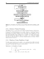
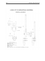
The basic conditions of the collision avoidance system in this thesis can be
summarized in Figure 4.1. The flowchart shows an example of how a suggested
27
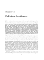
28
Collision Avoidance
Figure 4.1. Flowchart of Collision Avoidance System in the complete system. The
flowchart shows how the subsystems are connected and how they exchange information
with each other.
collision avoidance system could be implemented. This flowchart is an extension
of the flowchart in Section 2.5 and it has been divided into several subsystems.
All vehicles on the test track will have a communication device combined with
a trajectory prediction to estimate all other vehicles positions. An autonomous
vehicle also needs a vision system to take care of the unpredictable objects that
could occur (e.g. animals and items that are blocking the roadway).
4.1
Collision Avoidance Prediction
The prediction of the vehicle’s position is intended to estimate the risk of a future
collision. By using a model of the vehicle motion, the future position can be
predicted. There are several vehicle models that can be used for prediction of
the position with different degrees of complexity (e.g. general models and vehicle
specific models that handles vehicle dynamics) [31, 34, 60].
One of the simplest vehicle model is the constant velocity model given in Equation (4.1) and (4.2). This model describes a straight line between two measurement
updates. The model is based on four states as position (x and y) and constant
velocity in both directions (νx and νy ). This model will be used in some examples
in this report to show the principle of collision avoidance when the vehicle states
are known.
4.1 Collision Avoidance Prediction
29
Figure 4.2. Block diagram of the position states estimator
X(ti ) =
x(ti ) y(ti ) νx (ti ) νy (ti )
T
1 0 (ti+1 − ti )
0
0 1
0
(ti+1 − ti )
X(ti )
X(ti+1 ) =
0 0
1
0
0 0
0
1
(4.1)
(4.2)
All vehicle states are calculated by the vehicle itself and then transmitted to
all other vehicles which leads to the errors in the states being less than when these
states have to be estimated by the other vehicle. Another advantage is that the
vehicle does not need visual contact with the other vehicles to track and estimate
their future positions. Since all vehicles receive the vehicle states from the other
vehicles, the prediction will be the same, independent of which vehicle that does
the prediction. An example flowchart of how the states can be calculated is shown
in Figure 4.2.
When the states are known a prediction can be done. By comparing the prediction of a vehicle with the surrounding vehicles, a future possibility of a collision
can be predicted. If the vehicle model and the measurement of the states are really
good, an implementation of a collision avoidance system can be done by assigning
a safety area around the vehicles. When these areas overlap each other the system
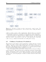
will alert. An example of this is shown in Example 4.1.
Example 4.1: Ideal linear prediction with fixed safety distance
30
Collision Avoidance
Two vehicles are traveling in the nearby area. Both are estimated with a constant
velocity model (see Equation (4.1) and (4.2)). The two vehicles each have a preset
safety radius, in this example these are set to four and six meters. The vehicle
initial states are given as below:
X1 (t0 ) =
X2 (t0 ) =
0
0
0 −55
10
10
0
T
10
T
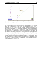
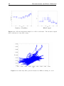
The predicted positions are presented in Figure 4.3. If both vehicles continue
with present headings and velocities, there is a great probability that a collision
will take place after five seconds. The future predictions in this case require a
perfect model and state estimation.
Figure 4.3. A linear prediction from the present position at x̂(0|0). Circles around
every prediction symbols the fixed safety distance. At state x̂(5|0), the two position
estimations with corresponding safety distances will indicate a possible collision.
In Example 4.1, the model as well as the measurement are assumed to be be
very good and are not very realistic. Almost all state measurement equipments
have some kind of errors (see Table 2.1 for typical GPS accuracy) and this insecureness should be taken into consideration. In Example 4.2, an error in the
position is assigned and the safety area is then increased in each step.
4.1 Collision Avoidance Prediction
31
Figure 4.4. Linear prediction with increasing prediction error. In every prediction, the
safety distance is increased. Circles around every prediction symbols the safety distance.
At state x̂(5|0), the two position estimations with corresponding safety distances will
indicate a possible collision.
Example 4.2: Linear prediction with error in position
The situation is identical to the situation in Example 4.1 and the vehicle states
are the same. The vehicle position has an error due to uncertainty in the position
system. This will lead to a greater uncertainty of the future predicted positions.
The probability of a future collision will also increase. The error in position is
defined as σx2 = 0.5m and σy2 = 0.5m
To cover the predicted area with a safety distance, the radius is enhanced for
every step in time. By using the standard deviation to predict the worst case
2
scenario, an area could be calculated with σx,y
· k. An example is showed in Figure
4.4.
Another technique to estimate the future position is to use the Kalman m-step
prediction. By calculating the error covariance matrix (P ) and the state vector
x̂ (see Algorithm 1) and then performing the m-step prediction (see Algorithm
2) with these variables, the future states can be estimated. This calculation also
considers the given state and measurement errors (Q and R). If the noise is
assumed to be Gaussian it can be shown that the equation g = (x(t + m|t) − x̃(t +
m))T [P (t + m|t)]−1 (x(t + m|t) − x̃(t + m)) is a χ2 distributed variable [12, 29]. In
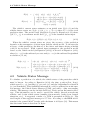
Example 4.3 a Kalman m-step prediction is done.
32
Collision Avoidance
Algorithm 1 Kalman filter (KF)
Initial values:
x̂(0| − 1) = x0
P (0| − 1) = Π0
Time update:
x̂(t + 1|t) = At x̂(t|t)
P (t + 1|t) = At P (t|t)(At )T + Qt
(4.3a)
(4.3b)
Filter gain computation:
L(t)
= P (t|t − 1)CtT [Ct P (t|t − 1)CtT + Rt ]−1
(4.4)
Measurement update:
x̂(t|t) = x̂(t|t − 1) + L(t)(y(t) − Ct x̂(t|t − 1))
P (t|t) = P (t|t − 1) −
P (t|t − 1)CtT [Ct P (t|t − 1)CtT + Rt ]−1 Ct P (t|t − 1)
(4.5a)
(4.5b)
where
Qt
Rt
= Cov(wt )
= Cov(et )
Algorithm 2 Kalman filter, m step predictor
x̂(t + m|t)
P (t + m|t)
= Am x̂(t|t)
= Am P (t|t)(Am )T +
(4.6a)
m
X
k=1
Am−k Q(Am−k )T
(4.6b)
4.1 Collision Avoidance Prediction
33
Example 4.3: Kalman prediction
By using the constant velocity vehicle model (see Equation (4.1)and (4.2)) and the
Kalman filter m-step prediction (see Algorithm 2), the future estimated position
and a confidence region around that prediction can be calculated. The constant
velocity model has been extended with process and measurement noise according
to the following equations.
1 0 1 0
1 0 0 0
0 1 0 1
0 1 0 0
x(t + 1) =
(4.7)
0 0 1 0 x + 0 0 1 0 ω
0 0 0 1
0 0 0 1
and
1
0
y=
0
0
0
1
0
0
0
0
1
0
0
0
x + ζ
0
1
(4.8)
where ω is normal distributed and has a covariance (σx,y = 0.5, σvx ,vy = 0.1)
σx 0
0
0
0 σy
0
0
Q=
0
0 σ vx
0
0
0
0 σ vy
and ζ has the covariance
1
0
R = Γ
0
0
0
1
0
0
0
0
1
0
0
0
0
1
(4.9)
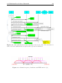
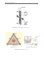
where Γ is small (0.0001) due to the communication possibilities. To determine
if the system should warn about a future collision risk, some definitions need to
be explained (see Figure 4.5). When the safety distance between two vehicles
is defined as Dth , it is of interest to know if two vehicles are separated with
at least Dth . When the noise is assumed to be Gaussian, the confidence region
around x(t) can be calculated. Due to the Gaussian noise the confidence region
g = (x(t + m|t) − x̃(t + m))T [P (t + m|t)]−1 (x(t + m|t) − x̃(t + m)) is a χ2 (n)
distributed variable where n is the dimension of x.
To determine the probability of the confidence region, a position x(t + m|t)
must be assigned. In this example the position
we have
chosen is the edge of
the ellipse with a radius of Rcalc = max D2th , D−2Dth . In the Figure 4.6, the
confidence region is plotted and the corresponding probability is shown in Table
4.1. If the probability is less than a given threshold, an indication of a future
hazard situation will be made. This indication can also be weighted with the step
number (m). A smaller m is a prediction in the near future and due to prediciton
errors it is a much greater risk for collision than if m is larger.
34
Collision Avoidance
Table 4.1. Position probability when using the Kalman prediction.
State x(t)
x(0|0)
x(1|0)
x(2|0)
x(3|0)
x(4|0)
x(5|0)
th
P x(t) ≤ D−D
2
≥ 99%
≥ 99%
≥ 99%
≥ 99%
≈ 50%
0 due to D ≤ Dth
Figure 4.5. Distance and angles defined for the Kalman prediction example.
4.1 Collision Avoidance Prediction
35
Figure 4.6. The Kalman position prediction.
In every
prediction, the confidence region
D D
is calculated according to Rcalc = max D2th , −2 th . With this information the system
is able to calculate the probability of the position estimation being within this region.
At state x̂(5|0), the two position estimations with corresponding confidence region will
indicate a possible collision.
36
Collision Avoidance
As shown in Example 4.1-4.3, the position prediction are exactly the same due
to no difference in the model. The difference of using the Kalman prediction is
that this technique handles the error in a more realistic way. Another advantage
of the Kalman technique is that the confidence interval of the prediction is χ2 distributed.
The vehicle model that is used in these examples is, as mentioned, very simple.
Increasing the model to a non-linear model also increases the accuracy of the calculated positions. The side effects are that the CPU-time increases and an extended
Kalman filter has to be used (see Appendix E for information of an extended
Kalman filter technique). The choice of model will depend of computing capacity
and demands of accuracy. By comparing very simple models, an indication can
be given of how the accuracy and computational demands are combined. By running several Monte-Carlo simulations (1000 MC simulations) and comparing the
average path on each model (Constant velocity, Constant acceleration, and Nearly
coordinated turn1 ), a grade of computional load can be achieved. An example is
presented in Table 4.2 [31].
By using non-vehicle dependent models, it is very easy to adapt the system
to a wide range of different vehicles. This increases the versatility of the system.
As seen in Table 4.2, the maximum error of for example the nearly coordinated
turn model (3.5 m) is acceptable as the safety radius will be greater than this
distance. In Equation (4.10)-(4.12) a suggested vehicle model is presented. The
suggested vehicle model is similar to the nearly coordinated turn model. In the
model, the variables x and y are earth inertial coordinates, ϕ is the heading angle,
νx is the longitudinal velocity, ψ̇z is the yaw rate, ψ̇b is the bias in the yaw rate
measurement, and ηψ̇b is a white Gaussian noise. This is a general model that is
independent of vehicle handling parameters. This model has shown good accuracy
in position and good performance in prediction [60]. By using this kind of model, it
is easy to assign it to a great number of different vehicle’s and it makes the system
very versatile due to the independence of the vehicles models. The accuracy could
of course be increased by extending the model with vehicle specific parameters, but
the versatility of the model and the accuracy should be enough for the intended
function as a collision avoidance predictor [59, 60].
1 See
[31] for more information about given vehicle models.
Table 4.2. Vehicle model errors and CPU time [31]
Model
Constant velocity
Constant acceleration
Nearly coordinated turn
RMSE2 [m]
0.88
0.65
0.56
Max error [m]
5.2
4.7
3.5
CPU time
1
1.2
2.8
4.2 Vehicle States Message
X(ti )
=
x(ti ) y(ti ) ϕ(ti ) ψ̇b (ti )
37
T
x(ti ) + (ti+1 − ti )νx (ti ) cos ϕ(ti )
y(ti ) + (ti+1 − ti )νx (ti ) sin ϕ(ti )
=
ϕ(ti ) + (ti+1 − ti )(ψ̇z (ti ) − ψ̇b (ti ))
ψ̇b (ti ) + ηψ̇b (ti )
X(ti+1 )
(4.10)
The vehicle’s current states estimates as an initial state Xp (tn , 0) and the
vehicles future states are Xp (tn , tp ), (0 ≤ tp ≤ Tpred ) where Tpred is the total
prediction time. The model based prediction is given by Equation (4.11) where
f (X, U, tn , tp ) is a nonlinear model and Up (tn , tp ) is the assumed future input.
Ẋp (tn , tp ) = f (Xp (tn , tp ), Up (tn , tp ), tn , tp )
(4.11)
When the vehicle’s current states are given, the accuracy of the prediction
depends on the assumption of driver input and the vehicle model. To increase the
accuracy of this prediction, the history of the driver and future driving schedule
could be incorporated. With constant input assumption, the prediction model
based on the vehicle model (in Equation (4.10)) is showed in Equation (4.12),
where (ψ̇z − ψ̇b ) is the unbiased yaw rate and (ax − ab ) is the unbiased longitudinal
acceleration [59, 60].
Xp (tn , tp )
=
x(tn , tp ) y(tn , tp ) ϕ(tn , tp ) νxp (tn , tp )
T
X(tn , tp+1 )
4.2
x(tn , tp ) + (tp+1 − tp )νxp (tn , tp ) cos ϕ(tn , tp )
y(tn , tp ) + (tp+1 − tp )νxp (tn , tp ) sin ϕ(tn , tp )
(4.12)
=
ϕ(tn , tp ) + (tp+1 − tp )(ψ̇z (tn ) − ψ̇b (tn ))
νxp (tn , tp ) + (tp+1 − tp )(ax (tn ) − ab (tn ))
Vehicle States Message
To calculate a prediction of a vehicle, the vehicle states of the particular vehicle
must be known. According to Equation (4.12), the time, position (Lat, Long),
vehicle speed (vx , vy ), heading (ϕ), yaw rate (ψ̇), and the longitudinal acceleration
(ax ) are demanded. This demanded information could be gathered in an information message, the Vehicle States Message (VSM), and sent to other surrounding
vehicles. This message can also include an ID tag, Track, and an Information Message. This information can be used to specify the vehicle, discard non-relevant
vehicles, and obtain vehicle status (running autonomously, brake down, hazard
situations, etc.). A suggested content of a VSM is presented in Table 4.3. The
total length of this suggested message is 157 bits. According to the IEEE 802.11
standard, the general MAC3 header with checksum is 30 Bytes [10]. This means
that the entire frame is less than 50 Bytes.
3 Media
Access Control
38
Collision Avoidance
Table 4.3. Vehicle State Message
Message information
Time
Lat
Long
North/South
West/East
Speed
Heading (ϕ)
Yaw rate (ψ̇)
Acceleration (ax )
ID
Track
Information Message
4.3
Range
[00:00:00.00,23:59:59.99]
[0.000 000,90.000 000]
[0.000 000,180.000 000]
North = 1, South = 0
West =1, East = 0
[0.00,100.00]
[0.0,360.0]
[-40.95,40.95]
[-20.00,20.00]
[0,255]
[0,255]
[0,255]
SI unit
Seconds
Degree
Degree
m/s
Degree
Degree/s
m/s2
Number of bits
25
27
28
1
1
14
12
13
12
8
8
8
Collision Avoidance Vision
A part of the collision avoidance system is the trajectory prediction technique.
This is implemented for all vehicles (autonomous and with human drivers). Even
if every vehicle has a communication system, a positioning system, and has connection with everyone, an unpredictable object can occur on the test track. An
animal can run across the roadway, a truck can lose its trailer, a vehicle can break
down, etc. A vehicle with a human driver can react to this scenario and do an
avoidance manoeuvre but an autonomous vehicle has to be extended with a vision system. For collision avoidance systems several different vision techniques are
used. The systems that we have been investigating are presented in Chapter 2.4.
The demands of the vision system in this case is to achieve a satisfactory field
of view (about 180◦ ) and detect objects in front of the vehicle. An ACC radar
sensor has normally a 15◦ field of view [31], but with this performance demand
a fusion unit (several sensors) or a custom specified radar must be used. The
lidar system has a greater field of view as well as the fusion unit. A single lidar
covers approximately 170◦ and a fusion unit (placed on each front corner) covers
approximately 300◦ [20, 26]. Figure 4.7 shows an example plot of a single lidar
detection area. The lidar is mounted on a truck’s front left corner. The dotted
line points out the field of view of a single lidar. The reflected image shows a
detection of a car in front of the vehicle. The high resolution makes it possible to
identify the object due to its significant structure. A fusion system also increases
the redundancy of the complete system. The data that is collected from the same
area makes it possible to verify the view of the front of the vehicle (the most
relevant area in the collision avoidance system) with a second measurement. The
sensor fusion also features as a backup if malfunction in one sensor should occur
[13].
A general feature in automotive collision avoidance systems is the possibility
of object tracking. The vision unit (e.g. radar or lidar) detects the object and
4.3 Collision Avoidance Vision
39
Figure 4.7. A front edge mounted laser scanner. The picture shows the echoes and how
the unit detects an object (in this case a car) in front of the vehicle
can observe a range to the object, a range rate measurement (e.g. by Doppler
shift), and an azimuth angle to the object. By estimating the vehicle states, a
prediction of the new position can easily be done. The predicted position can
then be used to determine how an avoidance manouvere should be implemented.
This is a feature that is relevant to use in regular traffic scenarios where every
surrounding vehicle is unknown [37]. In the case of test track environment and
surrounding conditions, the vehicle already has all the relevant vehicle states (from
the communication) and all vehicles are known. When surrounding vehicles states
are unknown, a tracking feature has to be implemented to observe the vehicles
states. Due to the already known vehicle states, a more precise prediction can
be done when the position and heading does not have to be estimated. Hence
this tracking feature can improve the avoidance manouvere if an unknown object
appears, e.g. an animal,a trailer,or a broken down vehicle. Further information
about tracking can be found in [11].
Chapter 5
Measurements and Data
Collection
In this chapter measurements and data collections that have been made during
the thesis are presented. The chapter will also cover analysis of the collected data
and signals.
5.1
GPS coverage
In this section the result of GPS coverage measurements is presented. It will cover
the results of long time static measurements, dynamic measurements at the tracks
at Hällered test site. Analysis of the GPS accuracy will also be handled.
5.1.1
Static GPS Coverage Hällered
To verify that the GPS coverage at Hällered is satisfactory, data was collected
during one week (see Table 5.1) with a stationary GPS receiver. The NMEA
GGA sentence (the NMEA sentence is specified in Appendix A.2) was monitored.
The receiver was placed with free sight in the Southern hemisphere direction. In
this test, a USB connected GPS receiver was used with a specification according
to Appendix F. In the GGA sentence contains several fields to determine the
GPS coverage (numbers of satellites) and quality (HDOP) of the GPS signal. To
obtain an accurate position the GPS receiver needs at least four satellites (see
Appendix A.2) and it needs to have an HDOP value below four for excellent
satellite constellation (see Appendix A.2).
Figure 5.1 shows is the number of satellites. It seems like it is several added
sinus waves with a large period time. To obtain a clearer signal, the signal is filtered
through a low pass Butterworth filter of the fourth degree with a cutoff frequency
of 10 mHz. In Figure 5.2, the filtered signal is plotted and the corresponding
frequency spectrum obtained through FFT1 calculation is shown in Figure 5.3.
1 FFT=Fast
Fourier Transform
41
42
Measurements and Data Collection
Table 5.1. Stationary GPS measurement
Date
Time
From
03/07/07
13:30
To
10/07/07
13:30
Figure 5.1. Number of satellites at Hällered sampled at 1 Hz during one week.
The frequency spectrum shows four major frequencies where the shortest period
time is approximately 24 hours.
The HDOP value recieved during this time is plotted in Figure 5.4 and the
figure shows that the value variates between approximately one and seven.
The conclusion from static measurements at Hällered is that the satellite coverage is satisfactory, but the HDOP value sometimes exceeds over the recommended
for excellent satellite constellation.
5.1.2
Test Track GPS Coverage
The different test tracks at Hällered are surrounded with trees (see aerial photo in
Figure 5.5). Therefore it is important to investigate if there are any GPS shadows
on the test track due to the vegetation and/or the topography. A GPS antenna
was placed on the center on the roof of an estate car and the NMEA GGA sentence
was logged during the test. The test was performed by driving laps on every single
lane of the test track to detect GPS shadows. The results are shown in Figure 5.6
and Figure 5.7. The results shows that the numbers of satellites and the HDOP
5.1 GPS coverage
43
Figure 5.2. Low pass filtered signal of the number of satellites at Hällered sampled at
1 Hz during one week.
Figure 5.3. Frequency spectrum of the low pass filtered signal in Figure 5.2.
44
Measurements and Data Collection
Figure 5.4. HDOP signal measured at Hällered sampled at 1 Hz during one week.
values are satisfying the demands for GPS navigation. With this result we know
that the tracks due not have any sections that suffer from GPS shadows. This
result shows that there should be no problem to use GPS as a positioning tool.
5.1.3
GPS Accuracy
To verify the GPS accuracy, three long-time, each one week of duration, measurements were made, one measuring at Hällered and two at Lundby. The GPS
receiver (see Appendix F for GPS receiver specifications) was located within clear
Southern hemisphere sight and mounted on a stationary platform. During the
measurements, the number of satellites was always at least four. Figure 5.8 shows
the position measured at Hällered plotted and Figure 5.9 - 5.10 the position measured at Lundby.
In Table 5.2 the drift is presented in meters (max2 , min3 and the standard
deviation (σ)). The distances between the points of interest where calculated
using the haversine formula (see Appendix D.1).
The standard deviation of all long-time measurements is close to the given
accuracy by the GPS manufacturer4 , but the maximum drift is almost fifteen times
higher. For autonomous positioning and navigation, both the standard deviation
and the maximum drift is of interest. Because the maximum drift is approximately
fifteen times higher than the standard deviation the lateral, longitudinal, and
Pn
Pi=1
n
3
2
xi
xn
+ max{x1 , x2 , . . . , xn } where n is the number of samples
− min{x1 , x2 , . . . , xn } where n is the number of samples
4 The GPS resolution given by the GPS manufacturer is the standard deviation
i
i=1 n
5.1 GPS coverage
45
Figure 5.5. Aerial photo of Hällered test site.
Number of Satellites
HDOP signal
Figure 5.6. GPS measurements sampled at 1 Hz on the Life Endurance Track.
Table 5.2. The GPS accuracy
Min
Max
σ
Hällered
Latitude Longitude
67 m
63 m
161 m
47 m
10 m
10 m
Lundby 1
Latitude Longitude
110 m
30 m
65
17 m
9
4m
Lundby 2
Latitude Longitude
186 m
30 m
94 m
70 m
10 m
5m
46
Measurements and Data Collection
Number of Satellites
HDOP signal
Figure 5.7. GPS measurements sampled at 1 Hz on all tracks. The measured signal
has no indication of any GPS outage.
Figure 5.8. Stationary GPS position measured at Hällered during one week.
5.1 GPS coverage
Figure 5.9. Stationary GPS position measured at Lundby (1)
Figure 5.10. Stationary GPS position measured at Lundby (2)
47
48
Measurements and Data Collection
Figure 5.11. Lat, Long, HDOP signals from Hällered.
HDOP signal is plotted in Figure 5.11 - 5.13. The figures shows that the position
seems to drift away when the HDOP value gets high. To reduce this position error
we have investigated if the position gets any better by removing some samples
when the HDOP value exceeds a given limit. In Figure 5.14 - 5.16 the result
is plotted and by removing approximately 300 samples the standard deviation is
reduced by approximately ten percent.
5.1.4
Dual GPS
The results in the static measurements indicated a drift in the static position. By
using two simple identical GPS receivers (data sheet in Appendix F) and logg
the measurements simultaneously, to investigate if both receivers were drifting to
the same position. In that case it might be possible to use one of them as a
local differential station. To see if the position varied together we investigated the
correlation (see Appendix D.2 for more information about these calculations) of
the signals. The results are presented in Table 5.3. It shows that the correlation
is small and that the signals do not follow each other closely. Due to the poor
result of this test the conclusion is that these GPS receivers are not suitable for
obtaining a local area correction.
5.1.5
Differential GPS
The test performed with a typical GPS receiver showed poor performance. To
verify if the cause of the poor performance was the hardware, a test using a high
5.1 GPS coverage
Figure 5.12. Lat, Long, HDOP signals from Lundby 1.
Figure 5.13. Lat, Long, HDOP signals from Lundby 2.
49
50
Measurements and Data Collection
Figure 5.14. Standard deviation improvement by removing samples for which HDOP
exceeds the given level (Hällered).
Figure 5.15. Standard deviation improvement by removing samples for which HDOP
exceeds given the level (Lundby 1).
Table 5.3. Correlation between the signals
Lateral
1.0000 0.3053
0.3053 1.0000
Longitudinal
1.0000 0.2434
0.2434 1.0000
5.1 GPS coverage
51
Figure 5.16. Standard deviation improvement by removing samples for which HDOP
exceeds given the level (Lundby 2).
performance differential GPS (with combined INS-system) was performed. The
DGPS receiver was a single antenna system with a standard deviation of 2 cm.
The measurements took place at Hällered and lasted for approximately 5 days.
See Appendix G and Appendix H for specification of the equipment used. The
DGPS/INS unit was mounted in an estate car with the antenna placed on the
roof of the car. The car was placed in a stationary position with a clear sky
and southern view. The position sample rate was set to 10 Hz. The position
data is presented in Figure 5.17. The position of the stationary measurement was
drifting from the static position. Our measurments show a standard deviation of
approximately 3.2 cm, which is larger than the specified 2 cm. The increase in
standard deviation is negligible due to the limited number of tests. The IMU in
the DGPS receiver should be connected with a fifth wheel to reduce some if the
drift in the position (see Figure 5.18). During the test performed for this thesis,
a fifth wheel was not available. Despite the advanced equipment, the system was
still drifting from the position, up to 23.5 m from the static position. This distance
is a worst case scenario. The plot of position (Figure 5.17) clearly shows that it
makes five different deviations from its static position. The HDOP signal was
not logged during this test, why the comparison between the drift and the HDOP
signal was not possible.
52
Measurements and Data Collection
Figure 5.17. Stationary DGPS position measurments at Hällered
Figure 5.18. Fifth Wheel for vehicle testing [27]
5.2 Laser Scanner Data Collection
53
Figure 5.19. Plotted lidar detection from the Volvo Integrated Safety Truck driving at
Lindholmen.
5.2
Laser Scanner Data Collection
Due to restricted availability to a lidar system, we were not able to perform these
measurements by ourselves. The data sequences which we have studied are from
the Volvo Integrated Safety Truck (VIST) at Volvo Technology. The data presented in Figure 5.19 is from a single, dual echo, four-layer technology laser scanner
mounted on the truck’s front left corner (see Appendix C.4.2 for more information). The angle of view is approximately 200◦ (dashed line in Figure 5.19). The
figure clearly shows the objects in the nearby area of the truck. In this particular
case it is an avenue with planted trees on both sides of the roadway. The left
side of the picture shows a wall. The conclusions of this data collection is that
the lidar is able to clearly detect and use the trees on the avenue as markings for
e.g. positioning. This points to the possibilities of using static known objects for
determining present position. In the picture some "objects", very near the front,
are occurring. This is dirt that are stuck on the laserscanner. This dirt can be
handled by filtering the signal.
Table 5.4. The DGPS accuracy
Drift
σ
Latitude
23.5m
3.2cm
Longitude
7m
3.1cm
54
5.3
Measurements and Data Collection
WLAN coverage
The distance coverage of a WLAN system is often specified by the manufacturers. The problem of these specifications is that the system is not applied in an
environment that is similar to a test track. In order to verify the capacity of the
WLAN system and get an indication of realistic working operating distances we
did several measurements at Hällered test site.
5.3.1
WLAN range
To verify the WLAN range, we mounted a WLAN Access Point (AP) (see Appendix I for technical specifications of the equipment) to an omni-directional antenna (see Appendix J for technical specifications of the equipment). The antenna
was mounted to a 3 m high pole to get good transference conditions (see Figure
5.20). The AP was connected to a laptop that constantly sent UDP messages at
a constant transfer rate. The receiving unit was mounted in an estate car with an
external antenna placed on the top center of the roof of the car. We drove the car
towards the AP to see at what maximum distance we could obtain a connection.
Figure 5.20. WLAN test base station.
During the test, the weather conditions were very moist and sometimes rainy.
These conditions were unfavourable for good WLAN coverage, although not a
worst case weather scenario. We also performed the test at different vehicle speeds
5.3 WLAN coverage
55
to investigate if the connection was dependent on the speed.
Distance test
To determine the maximum distance at which coverage communication could be
obtained, we drove against the antenna on a straight line and measured the distance with the odometer of the car. The first test speed was approximatly 60 km/h
and the distance from the AP was measured to approximately 600 m. When the
speed was reduced to approximatly 30 km/h the distance was measured to approximately 650 m when connection was established. During these tests the tendencies
of latency were less than 5 ms independant of the vehicle speed. The tests were
performed with constant visual contact with the AP.
Transfer Rate
During the tests a constant transfer rate was applied. The transfer rates that
we tested were 1, 2, and 11 Mbit/s. The distances of the AP range were near
constant for all tested transfer rates. In Section 4.2, the VSM is calculated to be
less than 50 Bytes, with header and checksum included. With a realistic usage
of 50 percent of the channel, the number of VSM’s that the system will be able
to send are presented in Table 5.5. With an update frequency of the VSM of
2 times per second and vehicle, the system will be able to handle at least 625
vehicles (calculated with the slowest transfer rate). A realistic assumption is that
the number of vehicles at the test site will be less than 100, which leaves room for
additional data transfer (e.g. measurement data).
Table 5.5. Messages per second
Tranfer rate
1 Mbit/s
2 Mbit/s
11 Mbit/s
50 % usage
0.5 Mbit/s
1 Mbit/s
5.5 Mbit/s
Number of messenges
1250
2500
13750
Environment
To see how the environment effects the connection possibilities, we drove around
the curve endurance track to see if we had similar coverage as in the distance test.
The curvature test results were not as good as the results of the straight line test.
When the test vehicle lost visual contact, the coverage distance rapidly decreased.
56
Measurements and Data Collection
Figure 5.21. AP position at Hällered endurance track during WLAN distance test.
Chapter 6
Conclusions
This chapter summarizes all systems and techniques which are mentioned in the
previous chapters. The advantages and disadvantages will be called to attention.
Systems and techniques which are suitable for autonomous implementation will be
presented and can bee seen as a recommendation for implementation or for future
investigations.
6.1
Positioning Conclusions
The positioning system is divided into two different parts, satellite positioning
and vision. These two systems are intended to be integrated by sensor fusion to
increase the performance and reliability of the complete system.
6.1.1
Positioning
To be able to drive autonomously, a positioning system is needed. This system
needs to be robust, precise, and redundant.
DGPS
A local area DGPS solution is the technique that offers the most advantages. The
possibility to increase the accuracy of more vehicles simultaneously is of great
advantage. The GPS coverage, in this case at Hällered, is satisfying (see section
5.1.1), thus a GPS positioning device would be suitable.
To make sure that the vehicle stays within one lane of the roadway, the accuracy
has to be less than one meter. To obtain the desired performance, a Differential
GPS (DGPS) with a carrier-phase technology (CDGPS) has to be used. The
accuracy of an CDGPS L1 receiver fulfills the demands of accuracy if the update
frequency is proportional to the vehicle speed. When driving with a speed of
up to 15 m/s, the update frequency has to be at least 20 Hz. When driving at
high speeds, a faster update frequence is needed. This can be achieved with more
sophisticated systems or in combination with INS systems.
57
58
Conclusions
Dilution of Precision
The GPS signal is very sensitive to the Geometric Dilution Of Precision (GDOP).
The test which has been done (see Section 5.1.3) shows that the accuracy can be
increased by isolating the time when the GDOP signal is high. Due to the orbits of
the satellites, the GDOP can easily be predicted and the reliability of the position
can be increased.
6.1.2
Vision
To obtain satisfactory robustness of an autonomous vehicle’s position, the use of
a vision system is needed. A good vision system is able to locate the position
by itself if the surrounding environment is known (lane marks, guidepoles, etc).
To obtain this feature a high resolution picture of the surrounding environment is
needed.
Lidar
The vehicle vision unit with most advantages for this application is a lidar system.
It provides a high resolution image with distances and bearing to objects and
obstacles. The lidar needs a multi echo feature to be able to reduce unwanted
detection (rain, fog, etc.) and a multi layer scanning to increase the resolution.
6.2
Communication Conclusions
The communication system needs to be robust with sufficient capacity to handle
all communication. It must be fast enough to reduce the risk of latencies in the
system.
6.2.1
WLAN
The WLAN technique is suitable for this implementation. The WLAN technique
is known as an "off the shelf technology". The great advantages of this is that
the technique is very cost efficient, and it still is under development with new
standards for future use, e.g. IEEE 802.11n. The test result when using a WLAN
shows that a significant distance can be covered with an omni-directional antenna.
However, there is a performance problem when the vegetation blocks the line of
sight between the AP and the receiving unit. To evade this problem, more AP’s
are needed to cover the complete area.
The Vehicle States Messages (VSM) size is very small compare to the transfer
rate. This indicates that the WLAN technique is suitable for future improvement
e.g. transferring the measurement data with the spared bandwidth.
6.3 Survaillence Conclusions
6.3
59
Survaillence Conclusions
Surveillance of all vehicles can be accomplished by using the VSM:s. The vehicles’
positions can be presented in real-time on a digital map. All additional information
in the VSM can also be presented as additional information about the vehicles.
With the VSM the current and predicted positions of the vehicles can be presented
to the traffic controller.
6.4
Collision Avoidance Conclusions
The suggested collision avoidance system is based on prediction of the future trajectory of the vehicle. This feature can be obtained by using a vehicle model and
with the information in the Vehicle States Message (VSM). A proposed VSM is
presented in Section 4.2. The prediction of any future trajectory conflict decreases
the possibilities of collisions.
To detect unpredicted objects a vision unit is needed. The lidar vison unit
supplies the system with a high detailed image and a large field of view to detect
objects in the nearby area.
These systems offer two different kinds of collision warnings. The warnings can
be presented to an autonomous vehicle as well as a warning to a human driver.
With these two systems, collision avoidance actions can be taken.
6.5
System Movability Conclusions
The recommended systems are movable because all of the systems are independent
of location. The positioning system is based on satellite navigation and a vision
unit which is integrated in the vehicle. The surrounding equipment such as the
differential base station and the WLAN AP’s can be placed on any desired test
area. If the test area is large or the topography causes communication losses in
some areas, more AP’s can be added to resolve this problem. The collision avoidance system is independent of location because the trajectory conflict is calculated
from the vehicle states and not based on a planned route conflict.
6.6
Future Work
This thesis work is based on literature and small scale testing. Many of the recommended systems are not tested by us in this thesis work. To verify the accuracy,
capacity, and adequacy under realistic conditions, further tests needs to be done.
6.6.1
Positioning System
In Measurement and Data Collection (Chapter 5) the maximum drift of the position is very large. It seems to be a correlation between the HDOP signal and
the position drift. As described in the chapter a simple filtering of the position
was made which increased the accuracy with approximately ten percent. By doing
60
Conclusions
more studies of the GDOP signals (HDOP, VDOP, PDOP and TDOP) and the
positioning drift, it might be possible to increase the position accuracy. The uncertanty of the position can be decreased if the GDOP signal is weighted and combined with additional sensors (e.g. IMU). Only a few tests with high performance
equipment has been done within this thesis work, and some of the conclusions
are based on low accuracy equipment and need to be verified using recommended
equipment.
6.6.2
Lidar System
The specifications of the lidar system is not yet validated to the testing environment of the test track (influence of vibrations, bad weather conditions, etc).
6.6.3
Communication System
The implementation, testing, and validation for the Dual Antenna system and
Neighbour Graph has not been done within this thesis.
Dual Antenna
To reduce the handover time when changing between AP’s we recommend a dual
antenna solution. The implementation of this technique should be done and verified.
Neighbour Graph
The neighbour graph technique might not be needed if the system is permanently
installed but it will make the system more adaptive to changes and disturbances
and make the system more movable due to the self building NG.
6.6.4
Collision Avoidance System
In this thesis work we have not investigated how the avoidance manoeuvre should
be preformed. This manoeuvre must be made in several different ways according
to different traffic situations (e.g. unknown object on the road, future trajectory
conflict, etc).
6.6.5
Fault Detection
In an autonomous vehicle the fault detection system must be extended. A human
driver can detect malfunctions in the vehicle which are not indicated by sensors
e.g. flat tire, drive shaft brake down, fire etc. To obtain this information more
sensors might be needed along with analysis of e.g. CAN data. Descriptions of
many of these errors and malfunctions can be gathered from interviewing the test
drivers about their experiences.
Bibliography
[1] Garmin 35/36 TracPak, GPS Smart Antenna, Technical Specification.
[2] CNS
Systems
AB.
Vdl
mode
4,
2007.
URL:
http://www.cns.se/aviation/core.php?page=aviation_technology_vdl
mode4.
[3] Neil Ackroyd and Robert Lorimer. Global Navigation. A GPS User´s Guide.
Lloyd’s of London Press Ltd, 2 edition, 1994.
[4] Fraport AG.
Tacsys/capts fraport project, 2007.
URL:
http://www.fraport.com/cms/company/dok/81/81480.tacsyscapts.htm.
[5] SICK AG. Homepage, 2007. URL: http://www.sick.com/home/en.html.
[6] The Defense Advanced Research Projects Agency. D.a.r.p.a challange, 2007.
URL: http://www.darpa.mil/grandchallenge/index.asp.
[7] The Defense Advanced Research Projects Agency. D.a.r.p.a home, November
2007. URL: http://www.darpa.mil.
[8] ZigBee Alliance. Zigbee alliance, 2007. URL: http://www.zigbee.org.
[9] David Andersson and Johan Fjellström. Vehicle Positioning with Map Maching Using Integration of a Dead Reckoning System and GPS. Master’s thesis,
Linköpings Universitet, ISY, Linköpings Universistet, 581 83 Linköping, 2004.
LiTH-ISY-EX-3457-2004.
[10] Dave Bagby, Bob O’Hara, and Dave Roberts. Proposed revisions to the mac
frame formats to support wireless distribution systems. Document 802.1194/248, 1994.
[11] Yaakov Bar-Shalom and William Dale Blair. Multitarge-Multisensor Tracking: Applications and Advances Volume III. Artech House, Inc., 2000.
[12] Yaakov Bar-Shalom, X. Rong Li, and Thiagalingam Kirubarajan. Estimation
with Applications to Tracking and Navigation. John Wiley & Sons, Inc., 2001.
61
62
Bibliography
[13] Alberto Broggi, Stefano Cattani, Pier Paolo Porta, and Zani Paolo. A
laserscanner-vision fusion system implemented on the terramax autonomous
vehicle. Intelligent Robots and Systems, 2006 IEEE/RSJ International Conference, pages 111 – 116.
[14] Jin Chen, Stefan Deutschule, and Kay Fuerstenberg. Evaluation methods and
results of the intersafe intersection assistants. Intelligent Vehicles Symposium,
2007 IEEE.
[15] Yin-Jun Chen, Ching-Chung Chen, Shou-Nian Wang, Han-En Lin, and Hsu
Roy C. Gpsensecar -a collision avoidance support system using real-time gps
data in a mobile vehicular network. Systems and Networks Communication,
2006. ICSNC ’06. International Conference.
[16] Dale
DePries.
Nmea
data,
2007.
http://www.gpsinformation.org/dale/nmea.htm.
URL:
[17] Andreas Eidehall. Tracking and threat assessment for automotive collision
avoidance. Phd thesis, Linköpings Universitet, Department of Electrical Engineering, Linköpings Universistet, 581 83 Linköping, 2007.
[18] Matts Eriksson and Jonas Lundmark. Tecnical Verification and Validation
of ADS-B/VDL Mode 4 for A-SMGCS. Master’s thesis, Linköpings Universitet, Department of Science and Technology, Linköpings Universistet, 601 74
Norrköping, 2002. LiTH-ITN-KTS-EX–02/34–SE.
[19] ESA.
European space agency:
Egnos,
2007.
http://www.esa.int/esaNA/GGG63950NDC_egnos_0.html.
URL:
[20] Andreas Ewald and Volker Willhoeft. Laser scanners for obstacle detection
in automotive applications. Intelligent Vehicles Symposium, 2000. IV 2000.
Proceedings of the IEEE, pages 682 – 687.
[21] FAA.
Federal aviation administration :
Waas, 2007.
http://www.faa.gov/airports_airtraffic/technology/waas/.
URL:
[22] Jay Farrell and Matthew Barth. The Global Positioning System & Inertial
Navigation. The McGraw-Hill Companies, Inc., 1998.
[23] Daniel Fredriksson and Anders Schweitz. Tecnical Verification and Validation
of TIS-B using VDL Mode 4. Master’s thesis, Linköpings Universitet, Department of Science and Technology, Linköpings Universistet, 601 74 Norrköping,
2004. LiTH-ITN-KTS-EX–04/013–SE.
[24] Kay Ch. Fuerstenberg, Klaus C.J. Dietmayer, and Volker Willhoeft. Pedestrian recognition in urban traffic using a vehicle based multilayer laserscanner.
Intelligent Vehicle Symposium, 2002. IEEE, 1:31 – 35.
[25] Bin Gao and Benjamin Coifman. Vehicle identification and gps error detection
from a lidar equipped probe vehicle. Intelligent Transportation Systems, 2006.
Proceedings. 2006 IEEE, pages 1537 – 1542.
Bibliography
[26] Ibeo Automobile Sensor GmbH.
Homepage,
http://www.ibeo-as.com/english/default.asp.
[27] PEGASEM Messtechnik GmbH.
Pegasem wheel,
http://www.pegasem.de/english/mainframe_uk.htm.
63
2007.
2007.
URL:
URL:
[28] Mohinder S. Grewal, Lawrence R. Weill, and Andrews Angus P. Global Positioning Systems, Inertial Navigation, and Integration. John Wiley and Sons,
Inc, 2001.
[29] Fredrik Gustafsson, Lennart Ljung, and Mille Millnert. Signalbehandling.
2001.
[30] Bernhard Hofmann-Wellenhof and Herbert Lichtenegger. GPS Theory and
Practice. 5 edition, 2001.
[31] Jonas Jansson. Collision Avoidance Theory with Application to Automotive
Collision Mitigation. Phd thesis, Linköpings Universitet, ISY, Linköpings
Universistet, 581 83 Linköping, 2005.
[32] Christopher Jekeli. Inertial Navigation Systems with Geodetic Applications.
Walter de Gynter GmbH & Co. KG, 2001.
[33] Anders Johansson. Kommuniaktionsgränssnitt mot GP&C transponder. Master’s thesis, Linköpings Universitet, Department of Science and Technology,
Linköpings Universistet, 601 74 Norrköping, 2003. LiTH-ITN-EX–03/005–SE.
[34] Rickard Karlsson. Simulation Based Methods for Target Tracking. Lic thesis,
Linköpings Universitet, ISY, Linköpings Universistet, 581 83 Linköping, 2002.
[35] Jörg Kibbel, Winfried Justus, and Kay Fürstenberg. Lane estimation and
departure warning using multilayer laserscanner. Intelligent Transportation
Systems, 2005. Proceedings. 2005 IEEE, pages 607 – 611.
[36] Hye-Soo Kim, Sang-Hee Park, Chun-Su Park, Jae-Won Kim, and SungJea Ko. Selective channel scanning for fast handoff in wireless lan using
neighbor graph. July. The 2004 International Technical Conference on Circuits/Systems, Computer and Communications (ITC-CSCC2004), Japan.
[37] Alexander Kirchner and Christian Ameling. Integrated obstacle and road
tracking using a laser scanner. Intelligent Vehicles Symposium, 2000. IV
2000. Proceedings of the IEEE, pages 675 – 681.
[38] Joo-Chul Lee and Dominik Kaspar.
Pmipv6 fast handover for
pmipv6 based on 802.11 networks.
Technical report, ETRI, 161
Gajeong-dong Yuseong-gu Daejeon, 305-700 Korea, July 2007.
URL:
http://tools.ietf.org/id/draft-lee-netlmm-fmip-00.txt.
[39] Oxford Technical Solutions Limited. Oxford technical solutions rt4000, 2007.
URL: http://www.oxts.co.uk/default.asp?pageRef=63.
64
Bibliography
[40] Arunesh Mishra, Min-ho Shin, and William A. Arbaugh. Context caching using neighbor graphs for fast handoffs in a wireless network. INFOCOM 2004.
Twenty-third AnnualJoint Conference of the IEEE Computer and Communications Societies, 1:361–365, 2004.
[41] Arunesh Mishra, Min-ho Shin, and William A. Arbaugh. Improving the latency of 802.11 hand-offs using neighbor graphs. International Conference On
Mobile Systems, Applications And Services, pages 70 – 83, 2004.
[42] Novatel.
Novatel
gps,
2007.
http://www.novatel.com/Documents/Papers/ProPakV3.pdf.
URL:
[43] Takashi Ogawa and Kiyokazu Takagi. Road environment recognition using
on-vehicle lidar. Intelligent Vehicles Symposium, 2006 IEEE, pages 120 – 125.
[44] Toshiya Okabe, Takayuki Shizuno, and Tsutomu Kitamura. Wireless lan
network system for moving vehicles. IEEE Symposium on Computers And
Communications (ISCC 2005), (10):211 – 216.
[45] Omnistar. Omnistar, 2007.
URL:http://www.omnistar.nl/DesktopDefault.aspx?tabid=344.
[46] Jörgen Ott and Dirk Kutscher. Drive-thru internet: IEEE 802.11b for "automobile" users. IEEE Infocom 2004 Conference.
[47] Oxford Technical Solutions Limited, Oxford Technical Solutions Limited, 77
Heyford Park Upper Heyford,Oxfordshire OX25 5HD. RT3000 Inertial and
GPS Measurement System User Manual, revision: 060502 edition.
[48] Bradford W Parkinson and James J Spilker Jr. Global Positioning System:
Theory and Applications Volume II. American Institute of Aeronautics and
Astronautics Inc., 1996.
[49] California PATH. Path, california partners for advanced transit and highways,
2007. URL: http://www.path.berkeley.edu/.
[50] Jon Person. Writing your own gps applications: Part 2 - causes of precision
error, 2007. URL: http://www.developerfusion.co.uk/show/4652/2/.
[51] Martin Pettersson. Distributed integrity monitoring of differential GPS corrections. Master’s thesis, Linköpings Universitet, ISY, Linköpings Universistet, 581 83 Linköping, 1998. LiTH-ISY-EX-2021.
[52] Andreas Rönnebjerg. A Tracking and Collision Warning System for Maritime Applications. Master’s thesis, Linköpings Universitet, ISY, Linköpings
Universistet, 581 83 Linköping, 2005. LiTH-ISY-EX-05/3709-SE.
[53] Sangho Shin, Andrea G. Forte, Anshuman Sing Rawat, and Henning
Schulzrinne. Reducing mac layer handoff latency in IEEE 802.11 wireless
lans. 2004. ACM 1-58113-920-9/04/0010.
Bibliography
65
[54] Jan Sparbert, Klaus Dietmayer, and Daniel Streller. Lane detection and
street type classification using laser range images. Intelligent Transportation
Systems, 2001. Proceedings. 2001 IEEE.
[55] Carsten Spichalsky. Golf gti 53+1 - the driverless car. dSpace News, (1):18–19,
2007.
[56] Swepos.
Swepos :
Glonass,
November 2007.
http://swepos.lmv.lm.se/gps/glonass/glonass.htm.
URL:
[57] Swepos.
Swepos
produkter,
http://swepos.lmv.lm.se/index_prod.htm.
URL:
2007.
[58] Kiyokazu Takagi, Katsuhiro Moirikawa, Takashi Ogawa, and Makoto Saburi.
Lane recognition using on-vehicle lidar. Intelligent Vehicles Symposium, 2006
IEEE, pages 540 – 545.
[59] Han-Shue Tan and Jihua Huang. Dgps-based vehicle-to-vehicle cooperative
collision warning: Enginering feasibility viewpoints. IEEE Transactions on intelligent transportation system (Vol.7 No.4 December 2006), (7), 2006. 15249050.
[60] Han-Shue Tan and Jihua Huang. A low-order dgps-based vehicle positioning
system under urban enviroment. IEEE/ASME Transactions on mechatronics
(Vol.11 No.5 October 2006), (5), 2006. 1083-4435.
[61] Andrews Space & Technology.
Glonass, November 2007.
URL:
http://www.spaceandtech.com/spacedata/constellations/glonass_con
sum.shtml.
[62] S. Wender, T Weiss, and K. Dietmayer. Improved object classification of
laserscanner measurements at intersections using precise high level maps. Intelligent Transportation Systems, 2006. Proceedings. 2006 IEEE, pages 756 –
761.
[63] Yilin Xhao. Vehicle Location and Navigation Systems. Artech House, INC.,
1997.
[64] Tomas Zirn. Wimax öppnar ny väg in till bredbandskunderna, 2007. URL:
http://computersweden.idg.se/2.2683/1.112141.
Appendix A
Satellite Navigation
Satellite navigation technology is based on measuring the distance to different
satellites. With the information of the satellite position and distance, the user position can be calculated by triangulation. Today only one system is fully operative,
and it is the NAVSTAR GPS.
A.1
History
The first satellite navigation system was the Navy Navigation Satellite System
(NAVSAT), also called TRANSIT. The system was using six low-orbiting (1100
km) satellites. The position was calculated by measuring the change in frequency
of the satellites transmission as it speeds past in low orbit. Because the system
only had six satellites the average time between the position update was about 90
min. The position accuracy was about 250 meter [3, 30].
A.2
GPS
The term GPS includes both the American system NAVSTAR (Navigation Satellite
Timing And Ranging Global Positioning System) and the Russian system GLONASS
(Global Navigation Satellite System) [3, 30].
NAVSTAR GPS
The GPS system is developed by the US DoD (United States Department of
Defense). The NAVSTAR GPS is divided into tree parts: the space segment,
the control segment and the user segment.
Space Segment
The space segment consists of 24 satellites arranged in 6 orbitals. The orbital
planes have an inclination angle of 55 degrees relative the earth equator. The
satellites have an average orbital altitude of approximately 20 200 km and i takes
67
68
Satellite Navigation
Table A.1. Location of the Components of the Operation Control Segment
Master control station
Master control station (backup)
Monitor station
Remote monitor station
Remote monitor station
Remote monitor station
Remote monitor station
Remote monitor station
Ground antenna
Ground antenna
Ground antenna
Ground antenna
Falcon Air Force Base, Colorado Springs, CO
Gaithersburg, MD
Falcon Air Force Base, Colorado Springs, CO
Cape Canaveral, FL
Hawaii
Ascension Island
Diego Garcia
Kwajalein
Cape Canaveral, FL
Ascension Island
Diego Garcia
Kwajalein
approximately 12 hours to complete one orbit. Each satellite have a precise atomic
clock and sends out messages with the current position, current time and an identity number. The satellites transmit on two frequencies centered on 1575.42 MHz
and 12227.60 MHz [3, 30].
Control segment
The control segment consists of six monitoring stations, four ground antennas and
a master control station. In Table A.1 is the control segment stations listed. The
control segment main purpose is to monitoring the health and status of the space
segment [3, 30].
User segment
The user segment provides the user with position, velocity, precise timing etc. To
provide this information the GPS receiver use an antenna and a receiver-processor.
The receiver-processor measures and decodes the satellite transmission.
Various GPS receivers uses different types of protocols to present the information. Some of the most common protocols is NMEA 0183, the Garmin protocol,
the SiRF protocol etc [3, 30].
Geometric Dilution Of Precision
The Geometric Dilution Of Precision (GDOP) describe the geometric strength of
the satellite configuration. A high number of satellites does not always indicates
that the position accuracy is high. To obtain an accurate positioning with GPS
navigation, the satellites have to be separated from each other. The GDOP value
is a measure of the error contributed by the geometric relationship of the satellites
positions. When the satellite are close together, the geometry is said to be weak
and the GDOP value is in this cases high. A low GDOP value represents a better
GPS positional accuracy due to the wider angular separation between the satellites
A.2 GPS
69
Figure A.1. Satellite constellation for good and poor Geometric Dilution Of Precision.
Table A.2. DOP value and rating
1
2-3
4-6
7-8
9-20
21-50
Ideal
Excellent
Good
Moderate
Fair
Poor
used to calculate a GPS units position (see Figure A.1). The ideal level is one,
and up to six is acceptable. The DOP values and rating are presented in Table
A.2.
The GDOP is divided into HDOP (Horizontal DOP), VDOP (Vertical DOP),
PDOP (Position DOP, 3-D) and TDOP (Time DOP). These values are presented
in different parts of the NMEA-code. These quantities follow mathematically from
the positions of the usable satellites on the local sky [48].
NEMA 0183
The NMEA 0183 is a standard the are based on serial communication. It has
one speaker and an optional number of receivers. It can be used by sonars, echo
sounder, gyrocompass, autopilot, GPS receivers and many other types of instruments. The GPS system uses the standard and is sends a string of information
(the most common are listed in Table A.3). One of the NMEA sentences is the
GPGGA (GGA) sentence which is a essential fix data which provide 3D location
and accuracy data. It includes information as the position (Latitude, Longitude),
fix quality, number of satellites being tracked, horizontal dilution of position, altitude, mean sea level, time in seconds since last DGPS update, DGPS station ID
number and a checksum data, see Table A.4 for example [16].
70
Satellite Navigation
Table A.3. NMEA 0183
$GPAAM
$GPBOD
$GPBWW
$GPGGA
$GPGLL
$GPGSA
$GPGST
$GPGSV
$GPHDG
$GPHDT
$GPRMB
$GPRMC
$GPRTE
$GPVTG
$GPWCV
$GPWNC
$GPWPL
$GPXTE
$GPXTR
$GPZDA
$GPZFO
$GPZTG
Waypoint Arrival Alarm
Bearing, Origin to Destination
Bearing, Waypoint to Waypoint
Global Positioning System Fix Data
Geographic Position, Latitude/Longitude
GPS DOP and Active Satellites
GPS Pseudorange Noise Statistics
GPS Satellites in View
Heading, Deviation & Variation
Heading, True
Recommended Minimum Navigation Information
Recommended Minimum Specific GPS/TRANSIT Data
Routes
Track Made Good and Ground Speed
Waypoint Closure Velocity
Distance, Waypoint to Waypoint
Waypoint Location
Cross-Track Error, Measured
Cross-Track Error, Dead Reckoning
UTC Date/Time and Local Time Zone Offset
UTC and Time from Origin Waypoint
UTC and Time to Destination Waypoint
Table A.4. GGA Example
GGA - essential fix data which provide 3D location and accuracy data.
$GPGGA,123519,4807.038,N,01131.000,E,1,08,0.9,545.4,M,46.9,M„*47
Where
GGA
Global Positioning System Fix Data
123519
Fix taken at 12:35:19 UTC
4807.038,N
Latitude 48 deg 07.038’ N
01131.000,E
Longitude 11 deg 31.000’ E
1
Fix quality
08
Number of satellites being tracked
0.9
Horizontal dilution of position
545.4,M
Altitude, Meters, above mean sea level
46.9,M
Height of geoid (mean sea level) above WGS84 ellipsoid
(empty field) time in seconds since last DGPS update
(empty field) DGPS station ID number
*47
the checksum data, always begins with *
A.2 GPS
71
GPS position determination
To calculate the position the GPS receiver needs to know the position of the satellites and the time a message have traveled from the satellite. In two dimensions
the position U (x, y, t) can calculated according to Equation (A.1 - A.2) where n
is the satellite number and Rn is the distance to satellite n. To get the right position in the two dimensional case it takes three satellites and in the general case
four. The extra satellite is needed to synchronize the simple clock in the receiver
with the precise atomic clock in the satellites. A larger number of satellites would
provide better resolution (see Figure A.2 for an example) [28, 29, 51].
(Snx − Ux )2 + (Sny − Uy )2
Rn = c · ∆tn
Three satellite coverage
= Rn2
= c · (tn − t)
(A.1)
(A.2)
Six satellite coverage
Figure A.2. Position accuracy according to the number of satellites. When more
satellites are used in the position estimation, a higher accuracy can be achieved [50].
Accuracy
The GPS system is not exact in its position determination. There are several
factors of disturbance that generates errors in the positioning. An included feature
in the GPS system is Selected Availability (SA). This is a deliberately encoded
random error that occurs and generates an error of about 100 m. This signal is
now turned off and greater resolution is available to the general public.
The atmospheric conditions affect the speed of the GPS signals as they travel
through the atmosphere and ionosphere. The error of this effect is minimal when
the satellite is right above the receiver and the error effect increases when the
satellite is nearer the horizon due to the signal is affected by this during a longer
time. The ionospheric delay affects the speed of microwave signals differently based
on frequency, the receiver is able to reduce this effect with comparing different
72
Satellite Navigation
Figure A.3. Multipath example when the GPS signals are reflected on objects before
reaching the user [50].
frequency bands, L1(1575,42 MHz) and L2 (1227,6 MHz). Ionospheric delay is a
well-defined function of frequency and the total electron content (TEC) along the
path, so measuring the arrival time difference between the frequencies determines
TEC and thus the precise ionospheric delay at each frequency. This feature is
mostly applied on expensive survey-grade receivers [28, 29, 51].
Multipath is also an effect that causes inaccuracy. The signals reflects and
bounces of nearby objects and causes a difference in travel time (see Figure A.3).
Multipath effects are less severe in moving vehicles. When the GPS antenna is
moving, the false solutions using reflected signals quickly fail to converge and
only the direct signals result in stable solutions. Clock errors is another factor of
position error. The onboard clocks in the GPS satellites are extremely accurate,
but they do suffer from some clock drift. This results in some inaccuracy of
the position. All this faults summarize in an inaccuracy of approximately 15m
[28, 29, 51].
GLONASS
GLONASS (Global’naya Navigatsionnaya Sputnikovaya Sistema) is the russian
version of the GPS system. The GLONASS system has their own satellites (18
satellites at this point). The project started in 1976. The goal of this project was
to have global coverage by 1991 but has not reach this object yet. The system
rapidly fell into disrepair with the collapse of the Russian economy. In the end
of 2009 the GLONASS system would have 24 satellites up and running for the
wanted performance [56, 61].
Appendix B
Inertial Navigation Systems
Inertial navigation systems use an IMU (Inertial Measurement Unit). This is
a closed system that detect movement and acceleration with a combination of
accelerometers and angular rate sensors. The IMU detect the current acceleration
and the rate of change in the angular sensors (pitch, roll and yaw, see Figure B.1)
and sum these up to calculate the total change from the initial position. As a
stand-alone system it suffer from accumulated errors [47]. All inertial navigation
systems suffer from integration drift, as small errors in measurement are integrated
in progressively larger errors in velocity an especially position. Additional roll
error due to centripetal and Coriolis acceleration. The IMU is adding all detected
changes to the current position and any error is accumulated. It can be based
on several different techniques, e.g. gyro stabilized platforms (B.2) or strap down
platforms. The platforms are based on vibrating structure gyroscopes (B.3), fiber
optic gyros, ring laser gyros (B.4 (a)) and/or pendular accelerometers (B.4 (b)).
All of these solutions have their benefits and disadvantages [9, 22, 32, 63].
B.1
Dead Reckoning
Dead Reckoning (DR) is a primitive technique to determine the position of a
vehicle. If the starting position and all the previous displacement are known the
position can be calculated through:
N (k + 1)
E(k + 1)
Z(k + 1)
ψ(k + 1)
θ(k + 1)
=
=
=
=
=
N (k) + v(k)T cos(θ(k))cos(ψ(k))
E(k) + v(k)T cos(θ(k))sin(ψ(k))
Z(k) + v(k)T sin(θ(k))
ψ(k) + T ψ̇(k)
θ(k) + T θ̇(k)
(B.1)
(B.2)
(B.3)
(B.4)
(B.5)
where T is the sample time and, N , E and Z are the north, east and height
position coordinates. v is the velocity, ψ is the yaw angle, and θ is the pitch angle.
All the signals are supposed to be constant during one sample period [9, 22, 32, 63].
73
74
Inertial Navigation Systems
Figure B.1. Roll, pitch and yaw angles.
Figure B.2. Gimbaled Gyrostabilized platform.
B.1 Dead Reckoning
75
Figure B.3. Vibrating structure gyroscope.
a
Ring laser gyro
b
Pendular accelerometers
Figure B.4. Inertial gyro systems
Appendix C
Prototype Systems
The theory of driving vehicles autonomous is already implemented by different car
manufacturers.
C.1
PATH
An example of line follower is the American PATH project. The ambition of this
project is to have autonomous traffic on the highways in California. The technique
that being used is a magnetic trail that are built in the road. By putting magnets
in the road (sizes of a marker pen) placed with distances of approximately 11.2m the vehicle can follow the magnetic line. Using the magnetic domains of the
permanent magnets, the system is able to use them as an ID-tag. The vehicles are
able to sense the field strength and by this it can control the direction and speed
of the vehicle. This technique gives a longitudinal accuracy of less then 0.3m and
lateral less then 0.05m. Five magnetometers is placed beneath the vehicle, and by
signal processing the vehicle is able to determine its position. Due to the simple
path, the implementation is quite robust and can handle high speed driving. The
implementation of this system demands high effort in setting up the road with
magnets. Although the permanent magnets are at low cost but the path is very
static and variation of driving schedules are minimal [49].
C.2
VW Golf GTi 53+1
Volkswagen AG has made a prototype car called "Golf GTi 53+1 ". It is a fully
autonomous car that uses a laser scanner and a DGPS for navigation. The basic
use of this car is handling and brake tests due to its capability of precision driving.
By using the autonomous car, the repeating sequences is much more like an exact
duplicate then with a human driver.
The Golf GTi uses an Ibeo laser scanner mounted below the front license plate
for front vision. For positioning and navigation it uses a DGPS system, RT3002
from Oxford Technical Solutions. This is a combination system that are using
76
C.3 Team LUX
77
a DGPS beacon antenna and an inertial navigation system to obtain a very high
position update frequency. This sophisticated equipment supplies the car the exact
position in sub dm level (less then 2.5 cm). The track is limited by cones that
easily can be detected by the laser scanner. By using the vision of the car on a
scouting lap, the car stores the route of the track to compute the optimal driving
schedule. A MicroAutoBox from dSPACE is implemented to control the power
steering, brake booster and the accelerator pedal [55].
C.3
Team LUX
The Team LUX is Ibeo’s and SICK’s first D.A.R.P.A Grand Challenge team [6].
They are using a modified Volkswagen Passat and made it fully autonomous.
The car navigates by a DGPS (Omnistar [45]) i combination with three laser
scanners (Ibeo). The use of three laser scanners gives the car complete 360◦ vision
around the vehicle. This application make it possible to get an exact position
in combination with the DGPS without any INS systems. The use of the laser
scanner vision, it calculates its position from reference points in the near area.
This gives the system very little drift [5, 26].
C.4
C.4.1
Previous Volvo projects
LKAB
A previous project that has been implemented by AB Volvo is the autonomous
trucks that runs i the mine industry at LKAB. The projects purpose was to build
a number of trucks that was supposed to drive autonomous in a restricted area, it
included active steering and modification in existing control units. The navigation
was based on laser scanning. By placing reflectors in the specified route and using
laser scanners for detection, the system was able to navigate by building a local
reference network and keep the vehicle on a specified route.
C.4.2
VTEC Prototype truck
The Volvo Technology (VTEC) are working with a concept truck, the Volvo Integrated Safety Truck (VIST). This concept truck is equipped with several different
observation technologies, main purpose of collision avoidance. One of this features
are the lidar system. In Figure C.1, the VIST is shown and the circled area shows
the lidar system integrated in the front of the truck. The lidar is used for collision
avoidance and as a pre-crash system.
78
Prototype Systems
Figure C.1. The Volvo Integrated Safety Truck with lidar sensor implementation (circled).
Appendix D
Mathematics
D.1
Haversine Equation
The haversine function is given by Equation (D.1). By setting Equation (D.2) as
the variable h, we can easily calculate the distance d between the points of interest.
θ
haversin(θ) = sin2
(D.1)
2
haversin
D.2
d
R
= haversin(∆φ) + cos(φ1 ) · cos(φ2 ) · haversine(∆λ)
(D.2)
√
d = R · haversin−1 (h) = 2R · arcsin( h)
(D.3)
Covariance
Cov(X, Y ) = E((X − µ)(Y − ν))
ρX,Y =
Cov(X, Y )
σX σ Y
79
(D.4)
(D.5)
Appendix E
Kalman filter
E.1
Extended Kalman filter
The KF is made for a linear model. Many models are nonlinear function in either
the state or measurement update. To use the KF the system can be linearized
around the lastest state estimation, when this is done the KF can be applied
[12, 52].
Consider a system
x(t + 1) = f (x(t)) + ω(t)
y(t) = c(x(t)) + v(t)
(E.1a)
(E.1b)
where the function f (x(t)) and h(x(t)) represent nonlinear functions. To linearize
the states a first order Taylor series around the current state are used. This will
result in this approximation:
f (t) ≈ f (x̂(t|t)) + F (t) · (x(t) − x̂(t|t))
c(t) ≈ c(x̂(t|t − 1)) + C(t) · (x̂(t) − x̂(t|t − 1))
(E.2a)
(E.2b)
where
F (t)
=
C(t)
=
∂f (t) ∂x x=x̂(t|t)
∂c(t) ∂x (E.3a)
(E.3b)
x=x̂(t|t−1)
With these approximations Equation (E.1a) and (E.1b) can be rewritten as:
x(t + 1) = F (t)x(t) + f (x̂(t|t) − F (t)x̂(t|t) + ω(t)
y(t) = C(t)x(t) + c(x̂(t|t − 1)) − C(t)x̂(t|t − 1)
80
E.1 Extended Kalman filter
81
The new state update and measurement update now looks like:
x̂(t + 1|t) = F (t)x̂(t|t) + (f (x̂(t|t)) − F (t)x̂(t|t)) = f (x̂(t|t))
x̂(t|t) = x̂(t|t − 1) + K(t)(y(t) − h(x̂(t|t − 1) − C(t)x̂(t|t − 1)) − C(t)x̂(t|t − 1)
= x̂(t|t − 1) + K(t)(y(t) − h(x̂(t|t − 1))
The EKF is summerized in Algorithm 3
Algorithm 3 Extended Kalman filter, EKF
Initial values:
x̂(0| − 1)
P (0| − 1)
= x0
= Π0
Time update:
x̂(t + 1|t) = f (x̂(t|t))
P (t + 1|t) = F (t)P (t|t)(F (t))T + Qt
(E.6a)
(E.6b)
Filter gain computation:
L(t)
T
T
= P (t|t − 1)C(t) [C(t)P (t|t − 1)C(t) + Rt ]−1
(E.7)
Measurement update:
x̂(t|t)
P (t|t)
= x̂(t|t − 1) + L(t)(y(t) − c(x̂(t|t − 1))
= (I − L(t)C(t))P (t|t − 1)
(E.8a)
(E.8b)
where
F (t)
=
C(t)
=
∂f (t) ∂x x=x̂(t|t)
∂c(t) ∂x (E.9a)
(E.9b)
x=x̂(t|t−1)
and
Qt
Rt
= Cov(wt )
= Cov(et )
(E.10a)
(E.10b)
Appendix F
Globalsat
82
PRODUCT SPECIFICATION
USB GPS RECEIVER
BU-353
Ver 1.03
GlobalSat Technology Corporation
16, No.186,Chien 1 Road, 235Chung Ho City,Taipei Hsien, Taiwan ,R.O.C.
Tel: 886-2-8226-3799(Rep.)
Fax: 886-2-8226-3899
Web: www.globalsat.com.tw
E-mail:[email protected]
Page 1 of 4
BU-353specification ver1.03.doc
Product Feature
•
“SiRF starⅢ” high performance and low power consumption chipset
•
All-in-view 20-channel parallel processing
•
Built-in patch antenna
•
Very High sensitivity to satellite signal (Tracking Sensitivity:-159 dBm)
•
Extremely fast TTFF(Time To First Fix) at low signail level
•
Build-in SuperCap to reserve system data for rapid satellite acquisition.
•
Supported NMEA 0183 data protocol
•
Super-cohesive magnetic for mounting on the car
•
Water resisted and non-slip on the bottom
•
USB interface connection port
•
LED indicator for GPS fix or not fix
LED OFF:
LED ON:
Receiver switch off
No fixed, Signal searching
LED Flashing:
Position Fixed
Page 2 of 4
System Specification
Electrical Characteristics (Receiver)
Chipset
Frequency
C/A Code
Channels
Sensitivity
Accuracy
Position Horizontal
Velocity
Time
WAAS enabled
Datum
Datum
Acquisition Rate
Hot start
Warm start
Cold start
Reacquisition
Protocol
GPS Protocol
GPS Output Data
GPS transfer rate
Dynamic Condition
Acceleration Limit
Altitude Limit
Velocity Limit
Jerk Limit
Temperature
Operating
Storage
Humidity
Power
Voltage
Current
SIRF Star III
L1, 1575.42 MHz
1.023 MHz chip rate
20 channel all-in-view tracking
-159 dBm
10m 2D RMS (SA off)
0.1m/sec
1 micro-second synchronized to GPS time
5m 2D RMS
WGS-84
1 sec., average (with ephemeris and almanac valid)
38 sec., average (with almanac but not ephemeris)
42 sec., average (neither almanac nor ephemeris)
0.1 sec. average (interruption recovery time)
Default: NMEA 0183
SiRF binary >> position, velocity, altitude, status and
control ;
NMEA 0183 protocol.supports command: GGA,
GSA, GSV, RMC, VTG, GLL (VTG and GLL are
optional)
Software command setting (Default : 4800,n,8,1 for
NMEA )
Less than 4g
18,000 meters (60,000 feet) max.
515 meters/sec. (1,000 knots) max.
20 m/sec**3
-40°~ 85°C
-40°~ 85°C
Up to 95% non-condensing
4.5V ~ 6.5V
80mA typical
Physical Characteristics
Dimension
USB Cable Length
53mm diameter , 19.2mm height
65"
Page 3 of 4
USB GPS Receiver
Due to continuous product improvements, all specifications may be subject to change without notice
Page 4 of 4
Appendix G
Oxford Tech RT 3002
87
RT3000
Inertial
and GPS
Measurement
System
Features
•
•
•
•
•
•
•
•
•
•
•
•
•
•
•
•
Export License Exempt
2cm Positioning
0.05km/h Velocity
10mm/s² Acceleration
Lateral Acceleration
0.03° Roll, Pitch
0.15° Slip Angle
0.01°/s Angular Rates
Other Measurements
Real-Time
Low Latency
CAN Output
Wheel speed input
500MB Logging
5 min Installation
Compact Size
Vehicle Applications
•
•
•
•
•
•
•
•
•
Vehicle dynamics
Autonomous vehicles
Roll-over testing
Lane change
NHTSA ESC
ITS testing
Simulation verification
Acceleration/braking
Lap timing, racing
RT3000 Inertial and GPS
Navigation System
The RT3000 Inertial and GPS
Navigation Systems are advanced six-axis inertial navigation systems, blended with
precision GPS, to give robust
outputs of position, orientation
and velocity.
The RT3000 Inertial and GPS
Navigation System includes
three angular rate sensors (gyros), three servo-grade accelerometers, a GPS receiver and
all the required processing in
one very compact box.
Six single GPS antenna models
in the RT3000 family allow us
to offer very competitively
priced products. The difference
between the products is the
positioning performance of the
GPS receiver, with our most
accurate model offering 2cm
accuracy.
The RT3000 works as a standalone, autonomous unit and
requires no user input before it
starts operating.
outputs are computed in realtime with a very low latency.
The outputs from the RT3000
Inertial and GPS Navigation
System are derived from the
measurements of the accelerometers and gyros. Using the
inertial sensors for the main
outputs gives the RT3000 system a high update rate (100Hz)
and a wide bandwidth. All the
The RT3000 Inertial and GPS
Navigation Systems outputs its
real-time measurements over
RS232, Ethernet and CAN bus.
Other Applications
• AHRS
• Video Correction
• Road Survey
Oxford Technical Solutions
77 Heyford Park
Upper Heyford
Oxfordshire
OX25 5HD
England
Tel: +44 1869 238 015
Fax: +44 1869 238 016
http://www.oxts.co.uk
mailto:[email protected]
Inertial+GPS
The precision ADC in the
RT3000 gives more than 20
bits of resolution. The resolution of the acceleration measurements is 0.12mm/s² (12μg).
The ADC oversamples the
analogue sensors and uses
coning/sculling motion compensation algorithms to avoid
aliasing of the signals.
Vehicle Dynamics Testing
Autonomous Vehicles
The CAN bus output can be
combined into a vehicle’s
CAN bus or captured using
any CAN data acquisition system. The real-time nature
allows the RT3000 to be used
for hardware in the loop and
controller development. Connection to powerful tools like
dSPACE is easy. CAN DBC
files are provided.
Aerial Survey Applications
The internal processing includes the strapdown algorithms (using a WGS-84 earth
model), Kalman filtering and
in-flight alignment algorithms.
Parameter
RT3200
RT3100
RT3020
RT3002
RT3050
RT3040
3.0mCEP SPS
1.4mCEP SBAS
1.0mCEP DGPS
1.8mCEP SPS
1.2mCEP SBAS
0.4mCEP DGPS
1.8mCEP SPS
1.2mCEP SBAS
1.5mCEP SPS
0.8mCEP SBAS
0.2m 1σ DGPS
0.02m 1σ DGPS
1.8mCEP SPS
1.2mCEP SBAS
0.5mCEP VBS2
1.5mCEP SPS
0.8mCEP SBAS
0.1mCEP HP2
0.2 km/h RMS
0.1 km/h RMS
0.08km/h RMS
0.05km/h RMS
0.08km/h RMS
0.07km/h RMS
10 mm/s² 1σ
0.01%
0.1% 1σ
100 m/s²
10 mm/s² 1σ
0.01%
0.1% 1σ
100 m/s²
10 mm/s² 1σ
0.01%
0.1% 1σ
100 m/s²
10 mm/s² 1σ
0.01%
0.1% 1σ
100 m/s²
10 mm/s² 1σ
0.01%
0.1% 1σ
100 m/s²
10 mm/s² 1σ
0.01%
0.1% 1σ
100 m/s²
Roll/Pitch
0.1° 1σ
0.05° 1σ
0.05° 1σ
0.03° 1σ
0.04° 1σ
0.03° 1σ
Heading
0.2° 1σ
0.1° 1σ
0.1° 1σ
0.1° 1σ
0.1° 1σ
0.1° 1σ
2 deg/hr
0.2 deg/√hr
100°/s
2 deg/hr
0.2 deg/√hr
100°/s
2 deg/hr
0.2 deg/√hr
100°/s
2 deg/hr
0.2 deg/√hr
100°/s
2 deg/hr
0.2 deg/√hr
100°/s
2 deg/hr
0.2 deg/√hr
100°/s
Track (at 50km/h)
0.2° RMS
0.1° RMS
0.07° RMS
0.1° RMS
0.1° RMS
0.08° RMS
Slip Angle
(at 50km/h)
0.3° RMS
0.2° RMS
0.15° RMS
0.15° RMS
0.15° RMS
0.15° RMS
Position Accuracy
Velocity Accuracy
Acceleration
– Bias
– Linearity
– Scale Factor
– Range1
Angular Rate
– In-run Bias
– ARW
– Range1
Lateral Velocity
0.3%
0.2%
0.2%
0.2%
0.2%
0.2%
Update Rate
100 Hz
100 Hz
100 Hz
100 Hz
100 Hz
100 Hz
Calculation Latency
3.9 ms
3.9ms
3.9 ms
3.9 ms
3.9 ms
3.9 ms
Note 1. 300m/s² and 300°/s options are available.
Note 2. A subscription is required to use OmniStar VBS and OmniStar HP Services.
The internal Pentium-class
processor runs QNX real-time
operating system to ensure that
the outputs are always delivered on time.
Inertial Sensors in RT3000 include servo-grade accelerometers
and precision MEMS angular rate
sensors. Powerful 40MHz floating
point DSP takes care of coning,
sculling and aliasing.
The Kalman filter monitors the
performance of the system and
updates the measurements
using GPS and wheel speed.
By using the measurements
from GPS, the RT3000 system
is able to maintain highly accurate measurements and correct
its inertial sensor errors.
The RT3000 comes with acquisition software that displays
the data on a PC or on Pocket
PC devices. The PC software
can be used to save tests in
files, display real-time results
and monitor the performance.
Simple configuration software
allows the user to change the
mounting angle; displace the
measurement point to a virtual
location; change the differential GPS options, etc.
Models
To choose the best model for
your application, think about
the positioning accuracy you
require and what differential
GPS corrections you can supply. OmniStar systems give
excellent results over a wide
area. The RT3002 can give
Parameter
Power
Dimensions (mm)
Weight
Magnetic GPS antenna for vehicle
mounting. Other types available.
The internal logging enables
the RT3000 to work standalone. Post-mission, data can
be output in ASCII text format
and loaded in to the software
of your choice.
Operating Temperature
Vibration
more accurate positioning in a
local area where licence-free
radios can be used to transmit
the corrections.
The RT3000 products are also
available as dual antenna models. Where accurate heading in
low dynamics is required, the
dual-antenna model may be
more suitable.
For further information please
contact Oxford Technical Solutions or your nearest local
agent.
RT3000
9-18 V d.c. 15W
234 x 120 x 80
2.2 kg
–10 to 50°C
0.1 g²/Hz 5-500 Hz
Shock Survival
100G, 11ms
Internal Storage
500 MB
Dual Antenna
No
Appendix H
Oxford Tech RT-Base
90
RT-Base
RT-Base GPS Base Station
Inertial+GPS
GPS
Base
Station
Features
•
•
•
•
•
•
•
•
•
•
45cm DGPS Corrections
20cm L1 Corrections
2cm L2 Corrections
RTCA Format
Integral 10h Battery
Integral Charger
Integral Mains PSU
Integral Radio Modem
450MHz Band
Error Correcting
Transmission
• Save/Restore Antenna
Position
• Multi-path Rejecting
GPS Antenna
• IP65 Rated Case
Compatibility
• RT3000
• RT4000
• RTCA
The RT-Base is a portable GPS
Base Station capable of providing Differential Corrections
for Differential GPS Receivers.
The RT-Base can be used with
the RT3000 products to give
up to 2cm positioning accuracy.
One RT-Base unit can be used
to correct multiple DGPS systems. Additional Remote Radio Modems can be purchased
for each mobile DGPS system.
Fast To Install
The RT-Base has been designed with installation speed
in mind. Simply connect the
GPS Antenna and the Radio
Modem Aerial; then turn on.
Qty
Oxford Technical Solutions
77 Heyford Park
Upper Heyford
Oxfordshire
OX25 5HD
England
Tel: +44 1869 238 015
Fax: +44 1869 238 016
http://www.oxts.co.uk
mailto:[email protected]
The unit can start transmitting
corrections in under 2 minutes
with a known location or under
5 minutes if the position needs
to be averaged.
Training for operators is also
minimal.
Instructions
are
printed on the inside of the
RT-Base unit and a Quick
RT-Base components with SATEL radio
1
RT-Base Unit
1
GPS-C006 15m GPS Antenna Cable
1
GPS-702-GG GPS Antenna
1
SATEL Satelline-3ASd Radio Modem
2
Radio Modem Aerial/Antenna with 3m cable
1
Lightweight Tripod
1
IEC Mains Cable
1
77C0002B Power Cable
1
Internal Radio Link – fit to use internal radio
1
RT-Base User Manual
1
RT-Base Quick Guide
Note 1: Different radios are required for operation in different countries
Guide is provided to make the
operation easy.
Integral Battery
The RT-Base includes a 10
hour battery for all-day operation. A 12-volt input is provided for an external battery if
required.
An internal mains charger can
charge the RT-Base’s battery
in 2 hours. The internal power
supply can be used to run the
system if mains power is available.
Multipath Rejection
The RT-Base uses PulseAperture Correlator Technology to minimise the effects of
multipath.
The GPS-700 Pin-Wheel Technology Antenna includes a
ground-plane to minimise
ground surface multi-path and
reflections.
Parameter
RT-Base Specifications
Mains Power
110-240 V AC. 50-60Hz. 3A Max.
Battery
12V, 7Ah, Sealed Lead-Acid
Charge Time
2 hours
Operating Time
> 10 hours
Operating Temperature
0 to 50°C
Charge Temperature
10 to 40°C
Environment
IP65 – with lid closed
Relative Humidity
95%, non-condensing
Corrections
RTCA (Differential, L1, L2)
Frequency
1 Hz
Format
RS232
Dimensions
486 x 392 x 192 mm
Weight
12.6 kg
Radio Modem
The RT-Base includes an internal radio modem. Several
options are available so that
the RT-Base can be used without a license in many countries.
The RT-Base includes a Remote
Radio Modem and Antenna for
use on the vehicle. The Radio
Modem in the RT-Base will be
factory configured for use in a
particular country or territory.
For correct operation of the RTBase it is essential to locate the
GPS antenna in a location
where it has a full view of the
sky, down to an elevation of 10
degrees in all directions. It must
also be away from reflective
objects, like buildings and trees.
Advanced Error Correcting
Codes are used in the Radio
Modem’s communication to
enhance reliability and minimise the number of corrupt
packets.
The Radio Modem provides
reliable transmission over a
2km range in an open environment. Since some packets
can be dropped or have errors,
the Radio Modem can be used
up to a range of 5km in open
environments.
IP65 Rugged Case
When the lid is closed the RTBase has IP65 ingress protection, making it suitable for use
in all weathers.
The RT-Base is mounted in a
rugged ultra high impact PELI
case.
For further information please
contact Oxford Technical Solutions or your nearest local
agent.
Radio
Details
SATEL
380 - 480 MHz band, up to 1 W, typically 5 km.
License free bands available for many European
countries. Radio will typically cover 8 bands
with 25 kHz channel spacing.
SATEL
869 MHz band, up to 500 mW, typically 2 km.
License free across most of European Union.
Freewave
900 MHz band, up to 1 W, typically >10 km.
License free in USA, Brazil, Canada.
Futaba
2.4 GHz band, 10 mW, maximum 2 km. License free in Japan.
Revision 070410. Subject to change without notice.
Appendix I
Cisco Aironet 1240G Series
Access Point
93
Data Sheet
Cisco Aironet 1240G Series Access Point
®
®
Cisco Aironet 1240G Series Access Points provide single-band 802.11g wireless
connectivity for challenging RF environments such as factories, warehouses, and large
retail establishments (Figure 1). Connectorized antennas, a rugged metal enclosure,
and a broad operating temperature range offer extended range and coverage versatility.
The Cisco Aironet 1240G Series provides local as well as inline power, including support
for IEEE 802.3af Power over Ethernet (PoE).
Figure 1.
Cisco Aironet 1240G Access Point
The Cisco Aironet 1240G Series is a component of the Cisco Unified Wireless Network, a
comprehensive solution that delivers an integrated, end-to-end wired and wireless network.
Using the radio and network management features of the Cisco Unified Wireless Network for
simplified deployment, the Cisco Aironet 1240G Series extends the security, scalability, reliability,
ease of deployment, and manageability available in wired networks to the wireless LAN (WLAN).
The Cisco Aironet 1240G Series is available in two versions: unified or autonomous. Unified
access points operate with the Lightweight Access Point Protocol (LWAPP) and work in
conjunction with Cisco wireless LAN controllers and the Cisco Wireless Control System (WCS).
When configured with LWAPP, the Cisco Aironet 1240G Series can automatically detect the bestavailable Cisco wireless LAN controller and download appropriate policies and configuration
®
information with no manual intervention. Autonomous access points are based on Cisco IOS
Software and can optionally operate with the CiscoWorks Wireless LAN Solution Engine (WLSE).
Autonomous access points, along with the CiscoWorks WLSE, deliver a core set of features and
can be field-upgraded to take full advantage of the benefits of the Cisco Unified Wireless Network
as requirements evolve.
All contents are Copyright © 1992–2007 Cisco Systems, Inc. All rights reserved. This document is Cisco Public Information.
Page 1 of 6
Data Sheet
Applications
Designed for rugged environments and installations that require antenna versatility, the Cisco
Aironet 1240G Series features antenna connectors for extended range or coverage versatility
and more flexible installation options. Manufacturing applications, for example, can place WLANs
in hazardous locations and remotely place antennas in those locations while securing the Cisco
Aironet 1240G Series Access Points.
The metal housing and industrial-grade components of the Cisco Aironet 1240G Series provide
the ruggedness and extended operating temperature range required in factories, warehouses,
“big box” retail environments, and similar facilities. High transmit power, receive sensitivity, and
delay spread for 2.4-GHz radios provide the long range and large coverage area consistent with
these applications. Access points can be placed above ceilings or suspended ceilings, allowing
antennas to be discreetly placed below drop ceilings. The UL 2043 rating of the Cisco Aironet
1240G Series allows for placement of the access points above ceilings in plenum areas regulated
by municipal fire codes. Public access applications such as large hotel buildings can also present
a challenging RF environment; the antenna versatility of the Cisco Aironet 1240G Series, together
with industry-leading range and coverage, provides reliable performance for the most demanding
environments.
Features and Benefits
Table 1 lists the features and benefits of Cisco Aironet 1240G Series Access Points.
Table 1.
Features and Benefits of Cisco Aironet 1240G Series Access Points
Feature
Benefit
802.11g radios
The access points provide 54 Mbps of capacity and compatibility with older
802.11b clients.
Dual RP-TNC antenna
connectors for 2.4-GHz radios
Antenna connectors support a variety of Cisco 2.4-GHz antennas, providing
range and coverage versatility.
Security
Authentication
Security standards
Wi-Fi Protected Access (WPA)
WPA2 (802.11i)
Cisco Temporal Key Integrity Protocol (TKIP)
Cisco Message Integrity Check (MIC)
IEEE 802.11 WEP keys of 40 and 128 bits
802.1X Extensible Authentication Protocol (EAP) types:
EAP Flexible Authentication via Secure Tunneling (EAP FAST)
Protected EAP Generic Token Card (PEAP GTC)
PEAP Microsoft Challenge Authentication Protocol Version 2
(PEAP MSCHAP)
EAP Transport Layer Security (EAP TLS)
EAP Tunneled TLS (EAP TTLS)
EAP Subscriber Identity Module (EAP SIM)
Cisco LEAP
Encryption:
Current support for 12
nonoverlapping channels, with
potentially up to 23 channels
Advanced Encryption Standard Counter Mode with Cipher Block Chaining
Message Authentication Code Protocol (AES CCMP) encryption (WPA2)
TKIP (WPA)
Cisco TKIP
WPA TKIP
IEEE 802.11 WEP keys of 40 and 128 bits
Lower potential interference with neighboring access points
simplifies deployment.
Fewer transmission errors delivers greater throughput.
All contents are Copyright © 1992–2007 Cisco Systems, Inc. All rights reserved. This document is Cisco Public Information.
Page 2 of 6
Data Sheet
Feature
Benefit
Rugged metal housing
Metal case and rugged features support deployment in factories, warehouses, the
outdoors (NEMA enclosure required), and other industrial environments.
UL 2043 plenum rating and
extended operating temperature
The access points support installation in environmental airspaces such as areas
above suspended ceilings.
Multipurpose and lockable
mounting bracket
The access points provide greater flexibility in installation options for site surveys,
as well as theft deterrence.
Support for both local and
inline power, including IEEE
802.1af PoE
Hardware-assisted
AES encryption
Power can be supplied using the Ethernet cable, eliminating the need
for costly electrical power line runs to remotely installed access points.
The access points can be powered by IEEE 802.3af PoE, Cisco Inline
Power switches, single-port power injectors, or local power.
The access points provide high security without performance degradation.
Product Specifications
Table 2 lists the product specifications for Cisco Aironet 1240G Series Access Points.
Table 2.
Product Specifications for Cisco Aironet 1240G Series Access Points
Item
Part Number
Specification
AIR-AP1242G-x-K9
AIR-LAP1242G-x-K9
Regulatory domains: (x = regulatory domain)
A = FCC
E = ETSI
P = Japan2
Customers are responsible for verifying approval for use in
their individual countries. To verify approval and to identify the
regulatory domain that corresponds to a particular country,
please visit: http://www.cisco.com/go/aironet/compliance
Not all regulatory domains have been approved. As they are
approved, the part numbers will be available on the Global
Price List.
Data rates supported
802.11g: 1, 2, 5.5, 6, 9, 11, 12, 18, 24, 36, 48, and 54 Mbps
Network standard
IEEE 802.11b and 802.11g
Uplink
Autosensing 802.3 10 and 100BASE-T Ethernet
Frequency band and operating channels
Americas (FCC)
2.412 to 2.462 GHz; 11 channels
ETSI
2.412 to 2.472 GHz; 13 channels
Japan2
2.412 to 2.472 GHz; 13 channels Orthogonal Frequency
Division Multiplexing (OFDM)
2.412 to 2.484 GHz; 14 channels CCK
Nonoverlapping channels
802.11b/g: 3 channels
Receive sensitivity (typical)
802.11g
1 Mbps: –96 dBm
2 Mbps: –93 dBm
5.5 Mbps: –91 dBm
6 Mbps: –91 dBm
9 Mbps: –85 dBm
11 Mbps: –88 dBm
12 Mbps: –83 dBm
18 Mbps: –81 dBm
24 Mbps: –78 dBm
36 Mbps: –74 dBm
48 Mbps: –73 dBm
54 Mbps: –73 dBm
All contents are Copyright © 1992–2007 Cisco Systems, Inc. All rights reserved. This document is Cisco Public Information.
Page 3 of 6
Data Sheet
Item
Specification
Available transmit power settings
802.11g
(Maximum power setting varies by channel and
according to individual country regulations.)
CCK:
OFDM
20 dBm (100 mW)
17 dBm (50 mW)
17 dBm (50 mW)
14 dBm (25 mW)
14 dBm (25 mW)
11 dBm (12 mW)
11 dBm (12 mW)
8 dBm (6 mW)
8 dBm (6 mW)
5 dBm (3 mW)
5 dBm (3 mW)
2 dBm (2 mW)
2 dBm (2 mW)
Range (typical)
–1 dBm (1 mW)
Indoor (distance across open
office environment):
Outdoor:
802.11g:
802.11g:
105 ft (32m) at 54 Mbps
120 ft (37m) at 54 Mbps
180 ft (55m) at 48 Mbps
350 ft (107m) at 48 Mbps
260 ft (79m) at 36 Mbps
550 ft (168m) at 36 Mbps
285 ft (87m) at 24 Mbps
650 ft (198m) at 24 Mbps
330 ft (100m) at 18 Mbps
750 ft (229m) at 18 Mbps
355 ft (108m) at 12 Mbps
800 ft (244m) at 12 Mbps
365 ft (111m) at 11 Mbps
820 ft (250m) at 11 Mbps
380 ft (116m) at 9 Mbps
875 ft (267m) at 9 Mbps
410 ft (125m) at 6 Mbps
900 ft (274m) at 6 Mbps
425 ft (130m) at 5.5 Mbps
910 ft (277m) at 5.5 Mbps
445 ft (136m) at 2 Mbps
940 ft (287m) at 2 Mbps
460 ft (140m) at 1 Mbps
950 ft (290m) at 1 Mbps
Measured with 2.2-dBi dipole antenna for 2.4 GHz
Compliance
Standards
Safety
UL 60950-1
CAN/CSA-C22.2 No. 60950-1
UL 2043
IEC 60950-1
EN 60950-1
NIST FIPS 140-2 level 2 validation
Radio Approvals
FCC Part 15.247
RSS-210 (Canada)
EN 300.328 (Europe)
ARIB-STD 33 (Japan)
ARIB-STD 66 (Japan)
AS/NZS 4268.2003 (Australia and New Zealand)
EMI and susceptibility (Class B)
FCC Part 15.107 and 15.109
ICES-003 (Canada)
VCCI (Japan)
EN 301.489-1 and -17 (Europe)
EN 60601-1-2 EMC requirements for the
Medical Directive 93/42/EEC
Security
802.11i, WPA2, WPA
802.1X
AES, TKIP
Other
IEEE 802.11g and IEEE 802.11a
FCC Bulletin OET-65C
RSS-102
All contents are Copyright © 1992–2007 Cisco Systems, Inc. All rights reserved. This document is Cisco Public Information.
Page 4 of 6
Data Sheet
Item
Specification
Antenna connectors
2.4 GHz
Dual RP-TNC connectors
Status LEDs
Status LED indicates operating state, association status, error
or warning condition, boot sequence, and maintenance status.
Ethernet LED indicates status of activity over the Ethernet.
Radio LED indicates status of activity over the radio.
Dimensions (H x W x D)
1.1 x 6.6 x 8.5 in. (2.79 x 16.76 x 21.59 cm)
Weight
2.0 lb (0.9 kg)
Environmental
Nonoperating (storage) temperature: –40 to 185°F (–40 to
85°C)
Operating temperature: –4 to 131°F (–20 to 55°C)
Operating humidity: 10 to 90 percent (noncondensing)
System memory
32 MB RAM
16 MB flash memory
Input power requirements
100 to 240 VAC; 50 to 60 Hz (power supply)
36 to 57 VDC (device)
Powering options
Local power
802.3 AF switches
Cisco higher-power switches capable of supporting 13W or
greater
Cisco Aironet power injectors (PWRINJ3 and PWRINJ-FIB)
Third-party PoE devices (must meet input power and power
draw requirements)
Power draw
12.95W maximum
Note: 12.95W is the maximum power required at the powered
device. If the access point is being used in a PoE configuration, the
power drawn from the power sourcing equipment will be higher by
some amount dependent on the length of the interconnecting
cable. This additional power can be as high as 2.45W, bringing
the total system power draw (access point and cabling) to 15.4W.
Warranty
90 days
Wi-Fi certification
System Requirements
Table 3 lists the system requirements for Cisco Aironet 1240G Series Access Points.
Table 3.
System Requirements for Cisco Aironet 1240G Series Access Points
Access Method
Description
Browser
Using the Web browser management GUI requires a computer running Internet Explorer
Version 6.0 or later, or Netscape Navigator Version 7.0 or later.
PoE
Power sourcing equipment is compliant with Cisco Inline Power or IEEE 802.3af,
and provides at least 12.94W at 48 VDC.
All contents are Copyright © 1992–2007 Cisco Systems, Inc. All rights reserved. This document is Cisco Public Information.
Page 5 of 6
Data Sheet
Ordering Information
To place an order, visit the Cisco Ordering Website at:
http://www.cisco.com/en/US/ordering/index.shtml
Table 4 lists the product part numbers for Cisco Aironet 1240G Series Access Points.
Table 4.
Product Part Numbers for Cisco Aironet 1240G Series Access Points
Part Number
Description
AIR-AP1242G-A-K9
802.11g non-modular Cisco IOS access point; RP-TNC; FCC configuration
AIR-AP1242G-E-K9
802.11g non-modular Cisco IOS access point; RP-TNC; ETSI configuration
AIR-AP1242G-P-K9
802.11g non-modular Cisco IOS access point; RP-TNC; Japan2 configuration
AIR-LAP1242G-A-K9
802.11g non-modular LWAPP access point; RP-TNC; FCC configuration
AIR-LAP1242G-E-K9
802.11g non-modular LWAPP access point; RP-TNC; ETSI configuration
AIR-LAP1242G-P-K9
802.11g non-modular LWAPP access point; RP-TNC; Japan2 configuration
Service and Support
Cisco offers a wide range of services programs to accelerate customer success. These innovative
programs are delivered through a unique combination of people, processes, tools, and partners,
resulting in high levels of customer satisfaction. Cisco services help you protect your network
investment, optimize network operations, and prepare your network for new applications to extend
network intelligence and the power of your business. For more information about Cisco services,
visit Cisco Technical Support Services or Cisco Advanced Services.
For More Information
For more information about the Cisco Aironet 1240G Series, visit http://www.cisco.com/go/wireless
or contact your local Cisco account representative.
Printed in USA
All contents are Copyright © 1992–2007 Cisco Systems, Inc. All rights reserved. This document is Cisco Public Information.
C78-401676-01 07/07
Page 6 of 6
Appendix J
Antenna Specifications
100
101
102
Antenna Specifications
Upphovsrätt
Detta dokument hålls tillgängligt på Internet — eller dess framtida ersättare —
under 25 år från publiceringsdatum under förutsättning att inga extraordinära
omständigheter uppstår.
Tillgång till dokumentet innebär tillstånd för var och en att läsa, ladda ner,
skriva ut enstaka kopior för enskilt bruk och att använda det oförändrat för ickekommersiell forskning och för undervisning. Överföring av upphovsrätten vid en
senare tidpunkt kan inte upphäva detta tillstånd. All annan användning av dokumentet kräver upphovsmannens medgivande. För att garantera äktheten, säkerheten och tillgängligheten finns det lösningar av teknisk och administrativ art.
Upphovsmannens ideella rätt innefattar rätt att bli nämnd som upphovsman
i den omfattning som god sed kräver vid användning av dokumentet på ovan beskrivna sätt samt skydd mot att dokumentet ändras eller presenteras i sådan form
eller i sådant sammanhang som är kränkande för upphovsmannens litterära eller
konstnärliga anseende eller egenart.
För ytterligare information om Linköping University Electronic Press se förlagets hemsida http://www.ep.liu.se/
Copyright
The publishers will keep this document online on the Internet — or its possible replacement — for a period of 25 years from the date of publication barring
exceptional circumstances.
The online availability of the document implies a permanent permission for
anyone to read, to download, to print out single copies for his/her own use and
to use it unchanged for any non-commercial research and educational purpose.
Subsequent transfers of copyright cannot revoke this permission. All other uses of
the document are conditional on the consent of the copyright owner. The publisher
has taken technical and administrative measures to assure authenticity, security
and accessibility.
According to intellectual property law the author has the right to be mentioned
when his/her work is accessed as described above and to be protected against
infringement.
For additional information about the Linköping University Electronic Press
and its procedures for publication and for assurance of document integrity, please
refer to its www home page: http://www.ep.liu.se/
c Erik Agardt
Markus Löfgren