Download as a PDF

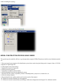
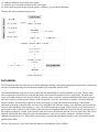
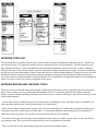
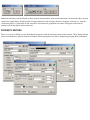
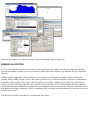
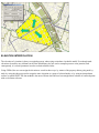
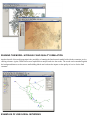
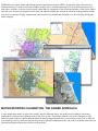
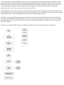
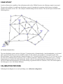
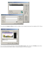
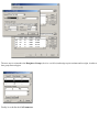
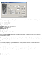
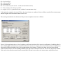
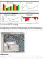
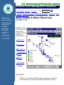
Hugo J. Bartolin, Fernando Martinez
Modelling and Calibration of Water Distribution Systems. A
New GIS Approach.
GIS is becoming an essential tool for utility companies, especially water companies, which have found an excellent way to
manage and assess their assets. This paper presents an ArcView® GIS extension called GISRed, which is a customized
application oriented to the task of water network modelling. GISRed is capable of simulating, analyzing and retrieving the
actual network status under certain conditions using an integration of the widely used EPANET engine. In addition to this, a
new functionality has been developed to allow the final user to calibrate the network model by means of a genetic algorithm
module which works seamlessly along with the extension. The final result is a full calibrated water network model derived
from the GIS database and ready to be used in decision making issues.
INTRODUCTION
Hydraulic simulation models are becoming of common use among planners, water utility personnel, consultants and many
other involved in analysis, design, operation or maintenance of water distribution systems. In order to make network
simulation models useful, it is necessary to calibrate them before being used (Walski, 1983; Ormsbee, 1989). The model
calibration process consists of adjusting a set of physical and operational parameters for the purpose of achieving a
reasonable match between measured and computed pressures and flows in the network. The integration of GIS and hydraulic
modelling software, offers many additional capabilities of analysis and data management. For this reason, it is not unusual to
see built-in applications that lump together GIS and hydraulic simulation/optimization software to obtain a valuable tool in
terms of modelling and decision-support. The benefits of the integration are quite evident. The modeler can save a lot of time
in constructing a network model making use of all the potential that the GIS offers when it comes to data management,
manipulation and analysis. On the other hand, the use of a hydraulic modelling software within the GIS environment provides
the advantage of simulating the model under any conditions, and analysing the model outputs in combination with other GIS
layers, and all, within the same environment. Optimisation methods have been widely used by engineers to calibrate networks
over the last few decades. Taking advantage of this integration, optimisation modules can also play an important role as part
of the modelling process. This paper presents an extension to ArcView that basically integrates hydraulic modelling tools, a
hydraulic simulation software and a hydraulic calibration module.
CUSTOM-BUILT APPLICATION
WHAT IS GISRED?
GISRed is an Extension to ESRI’s ArcView GIS software that integrates the widely used hydraulic modelling software
EPANET 2.0 and a calibration module based on a genetic algorithm, along with all the original GIS functions. This ‘built-in’
application was originally conceived to make water distribution network models, and be used besides, to perform complex
tasks such as importing a whole or partial network from an external source, creating a hydraulic network model and
automatically calibrating it.
The ArcView GISRed Extension is essentially a tool for helping the hydraulic engineer in the task of modelling water
distribution networks and in supporting decision-making issues based on the model, all within a GIS environment. The
extension consists of a series of scripts (over 450) programmed in Avenue, along with a series of dialogs (over 30). It is based
on the concept of scenario, which is a new type of document that appears in the project manager of ArcView once the
extension is loaded. A scenario is basically a view document of ArcView whose most important difference is the associated
database needed to set up a network model. Moreover, every scenario includes two basic themes required to construct a
model, namely, a node and a link theme. They contain all the necessary features and references to represent the network
model, including the topology.
MODEL CONSTRUCTION PROCESS USING GISRED
The typical steps the modeller will have to go through when using the GISRed Extension to build a water distribution model
are:
1. Draw a network representation of the distribution system from scratch using the editing tools or import it from a CAD file,
a shapefile or Epanet input file.
2. Check import errors (if necessary).
3. Simplify the network (if required).
4. Edit the network properties.
5. Interpolate elevations at selected nodes.
6. Allocate demands based on consumptions by streets.
7. Describe how the system is operated by means of demand patterns, pump curves, control rules, etc.
8. Select the analysis options.
9. Run a hydraulic/water quality analysis and view the results of the analysis.
10. Calibrate the network manually as a first approach.
11. Calibrate the network automatically by defining a calibration configuration and using the GA calibration module.
12. Send the calibration results back to the model.
13. Perform a new simulation and analyze the results again.
14. If the results are good enough, stop the process, otherwise, go on with the calibration.
The next flow chart summarizes the process:
DATA MODEL
The Extension emulates the behaviour of a relational database defining a functional configuration that provides a robust inner
structure to build and manage water distribution models fully compatible with EPANET.
The relational database comprises a series of tables that are linked based on a unique identifier (key field). The two main
tables are directly associated to the node and link themes and contain the graphic reference (shape field). The node table
refers to all nodal elements of the network, namely, junctions, tanks, reservoirs, upstream and downstream nodes of pumps
and valves and also contains general features such as internal id’s, user id’s, and a series of numeric values that define the
legend to display. This table also contains the connectivity degree of each node and the rotation angle of the symbol
associated to the node. In the link table, records refer to all graphic link elements, namely, pipes and short lines between the
'from-to' nodes that define either a pump or a valve. This table contains the topology of the network as well as the status of
pipes (open/closed). Each one of these tables is linked to other non-graphical tables that contain all the relevant properties of
the elements required by a model. Apart from the tables that refer to the network elements, there are some others that refer to
hydraulic options and other properties such as demand patterns, pump curves, quality parameters, simulation options,
calibration configurations, etc. These tables are necessary to generate the input data required by both, the simulator and the
optimization module.
The next figure depicts a part of the relational structure of the database used in GISRed.
NETWORK TOPOLOGY
The Extension allows to build a network from scratch or import a network from different information sources, which is the
most usual procedure. The application enables the user to import data from ArcView shapefiles, CAD drawings (dwg, dxf,
dgn), Epanet input files or even a whole database generated with the application (used to import old versions or damaged
projects). Each one of these formats implies a specific interpretation of the information in its origin. At the time of importing,
the data are read, filtered, debugged if needed, treated and stored as a RDB (relational database). During the process, the most
remarkable point lies in the fact of generating a coherent topology for the network and assuring the connectivity between
lines whose respective nodes fall within a specified tolerance. To accomplish this, the application adds the corresponding two
nodes every time a source line/polyline is originally read or drawn.
NETWORK EDITING AND CHECKING TOOLS
There are a series of advanced editing tools grouped in different tool bars that are directly dependant upon the current active
theme. That is similar to the way of working within standard ArcView, in which the graphical user interface and menu
options associated change depending on the document and current active theme of the project. The tool bars that may be used
with the application are:
- Link tool bar: allows to add/remove pipes to/from the model, edit and modify vertices and draw pipes by coordinates. All
these operations, preserving the topology and connectivity of the network.
- Node tool bar: allows to add junctions, pumps, valves, reservoirs and tanks, move nodes (and consequently all those pipes
connected to the node), connect pipes to a node, make ‘T’ connections and delete nodes (merging the corresponding two
pipes into just one if possible). It is possible to convert any node from one type to another.
- The tool bar for the pipe/device themes (non modelling oriented), works in a similar way but it does not take into account
any topology action. This is reserved for auxiliary devices not to be considered in the model.
- There are also tools to work with catalog images and to generate street address themes.
Additional tools have been developed to check network inconsistencies such as bad connections, unconnected nodes, network
connectivity (graph theory based) and out-of-range parameters such as length, diameter, roughness, material, etc. After the
verification process, if some node or link errors have been detected, a graphical error theme will appear in the table of
contents with all the details of the actual error.
PROPERTY EDITORS
There are a series of dialogs to enter the hydraulic properties of all the elements present in the network. Those dialogs include
a browser that allows to go from element to element. Element properties can also be assigned by grouping them beforehand.
Other dialogs comprise curve and pattern editors, control rules dialogs, analysis options, etc.
DEMAND ALLOCATION
As far as a water distribution system is concerned, the demand allocation is usually one of the most important and critical
tasks when modelling a network, to such an extent that a reliable allocation can make a big difference in terms of hydraulic
behaviour.
GISRed extension implements a demand allocation tool to assign a base demand to the model junctions, based on the
company billing records grouped by streets and a road segment theme. The total consumption of each street is distributed to
its segments proportionally to their length. Then, the application is capable of identifying the nodes of the model that are
closer to each one of the street segments; this is based on a spatial operation. At this time the demand allocation is done by
equally distributing the total demand assigned to each street segment to all those closest nodes. The unaccounted-for-water is
next added proportionally to demands. All this is straightforwardly performed by the allocation tool for each one of the zones
included in the system.
New allocation methods are intended to be implemented in the future.
ELEVATION INTERPOLATION
The elevation of a junction is always a required property when trying to simulate a hydraulic model. Even though node
elevations do not have any influence in the flow distribution, they are used to compute pressure at the junction, and
consequently, it is a basic parameter in order to obtain reliable results.
Using GISRed, the user can assign the elevation to a node in three ways: by means of the property editors going node by
node, by using the edit group tool to assign the same elevation to a group of selected nodes, or by using an interpolation
surface or spatial GRID. This last method is the most efficient when the user has enough data in a theme of scattered points
with an elevation reference.
RUNNING THE MODEL. HYDRAULIC AND QUALITY SIMULATION
Another benefit of the total integration is the possibility of running the final network model built with the extension, just by
clicking a button. Again, GISRed offers new capabilities to analyze and view the results. The results can be matched against
the background themes such as streets and building blocks and evaluate the impact on the quality of service for the final
customer.
EXAMPLES OF USE IN REAL NETWORKS
GISRed has been used to model and calibrate real water distribution systems (WDS), varying from large real networks to
medium-sized ones. The most useful task GISRed can help with, is in master planning issues. In a master plan project, the
main idea is to define a scenario for the network model and give a diagnosis of the current performance of the system. Based
upon this, new scenarios are proposed for the short and long term taking into account the variation of the population and the
new areas of expansion. Finally, enhancements on the network are planned and simulated to see the feasibility and support
action strategies.
WATER NETWORK CALIBRATION. THE GISRED APPROACH
A water distribution model, in order to be reliable, must be calibrated, that is, the model must be capable of accurately
predicting flow and pressure conditions at any point of the system. According to Shamir et al (1968), calibration of pipe
network systems consists of determining the physical and operational characteristics of an existing system. This is achieved
by determining various parameters that, when input into a hydraulic simulation model, will yield a reasonable match between
measured and predicted pressures and flows in the network.
As a first approach, a manual calibration may be carried out, taking advantage of all the capabilities of GISRed such as the
generation of new scenarios in which new assumptions and configurations may be taken into consideration. In the wake of
the manual calibration, a much more tuned calibration might be required. In this case, GISRed offers a module to fine-tune
some of the network parameters using an advanced search technique. This module is based on a Genetic Algorithm
developed by the Centre for Water Systems of the University of Exeter.
Genetic algorithms (GA) are one of the new evolutionary computing (EC) search techniques that have been developed in the
past thirty years. These search techniques utilise many of the evolutionary processes in nature, to find near optimum solutions
to real world problems. One of the most favourable of these EC search techniques is the GA.
Essentially, a genetic algorithm optimises a given function as long as it can be explicitly defined. GA’s mimic nature and
they carry out this with the representation and the operators. As far as the representation is concerned, GAs use a coding to
the problem similar to that of DNA's. The process is based on operations that emulate the natural selection, crossover and
mutation techniques.
The process to calibrate a WDS using the GA calibration module can be summarised by the following diagram:
CASE STUDY
In order to illustrate the capability of the calibration module of the GISRed Extension, the following example is presented.
The network to calibrate is a small water distribution system of a hypothetical community called Anytown (originally
introduced by Walski et al in 1987). This example is installed along with the extension. The network layout is shown in the
following picture:
NETWORK PROPERTIES
The water distribution system consists of 40 pipes, 22 junction nodes (16 demand nodes, 6 non-demand nodes), two elevated
tanks, one fixed head source (reservoir) and three pumps. For this example, pipe roughness is expressed in terms of the
Hazen-Williams C factor. Both tanks have bottom elevations of 65.5 m and overflow elevations of 79.5 m. The water level in
the clear-well is maintained at an elevation of 3.04 m. All three pumps have identical pump characteristic curves. A unique
demand pattern is considered for all demand nodes. Besides, there are four monitoring points located on nodes 40, 90, 120
and 140 at which head measurements were recorded during a hypothetical field test. (Ormsbee, 1989). The initial roughness
for all the pipes is set to 100 (Hazen-Williams).
CALIBRATION PROCESS
Following the last diagram, let us start by defining a new calibration configuration:
Let us select the Loading Conditions for which to calibrate. In this example the duration of the simulation will be 24 hours.
Let us specify the monitoring points that recorded the Head Measurements. This is done in the Field Data section. Since
there are just head measurements available, a head measurement text file will be imported.
The next step is to introduce the Roughness Groups (decision variables) and assign a prior estimate and a weight, in order to
later group network pipes.
Finally, let us define the GA Parameters.
In this example we are going to use Integer Genes that can take the values from within a finite interval. For the genetic
algorithm the following parameters are selected:
GA Type: STEADY STATE
Selector: TOURNAMENT
Replacer: WEAKEST
Crossover: SIMPLE ONE POINT Rate: 0.90
Mutator: RANDOM Rate: 0.10
Population Size: 200
Random Seed: 3
Output Interval: 10
Max. Iterations: 1000
Min. Required Fitness Variance: 1E-6
At this point, pipe grouping is required, thus, using the Group Edit Dialog, we can assign the pipes to one of the groups of
roughness already defined.
The next step is the generation of the calibration input files. These files will allow the GA calibrator to do its job. After
running the calibrator, and once the optimization process ends, the results are imported into the database and a total fitness is
given for the problem configuration.
The problem is formulated as a constrained optimization problem of weighted least square type, (that is, minimise the
objective function E), subject to a particular set of nodal demands (loading conditions) and known boundary conditions
(reservoir/tank heads, pump/valve status).
where:
E = Fitness (dimensionless)
H* = Measured Head
H = Predicted Head
Q* = Measured Flow
Q = Predicted Flow
d* = Prior estimate of the decision variable (Pseudo Measurement)
d = Prior estimate of the decision variable
w = weights (1/s2), s = generalized error (residual, in measurement units)
In this particular example, the terms of flows and prior estimates are neglected, since we did not consider flow measurements
and the weights for all decision variables were set to 0.
The results presented after the calibration of the previous example network are as follows:
First of all, the application shows a list of roughness coefficients that better fit the network configuration. In addition, there is
also valuable graphic information to assist the modeller. For instance, in the next picture, the first chart shows the differences
between the predicted roughness for all pipe groups and the prior estimates. The next two charts show the observed and
predicted measurements (for each loading condition) with and without confidence intervals. The last one depicts the residual
values at the selected measurement location, namely the difference between observed measurements and predicted ones.
APPLICATION TO A REAL NETWORK
The GA module has been successfully applied to calibrate the water network of Valencia (Spain), which is a coastal city of
about 400,000 consumers. The network is around 1,200 km in length and unlike the majority of conventional networks, the
main characteristic of the Valencia system is that it is driven by valves, which makes the calibration particularly complex,
because of the different pressure zones that 3 different fronts of valves originate.
CONCLUSION
The capabilities of a GIS can be extended beyond that of maintaining utility records into the area of planning and managing.
It is becoming more and more popular to use computer models to simulate the reality before taking any decision. This also
applies to water companies, which employ water models to ensure the adequate quantity and quality service of the drinking
water to the community.
The use of ArcView GIS along with the additional functionality given by a customized extension oriented to water
distribution network modelling, may suppose a major advance in terms of analysis, assessment and maintenance of the main
assets of a water company. The integration of a hydraulic simulator within a GIS, offers a series of advantages for the water
engineer, not only in terms of evaluation of the system performance, but also at other levels, such as, planning, design,
management and decision-making issues.
Consequently, an ArcView GIS extension called GISRed has been developed to fulfil these objectives. It has been used in
many projects, from large to medium-sized urban areas, to diagnose the state and performance of the water network system,
so that many alternatives can be studied before taking any real action on the system.
ACKNOWLEDGMENTS
This project has been developed within the REDHISP group from the Hydraulic Engineering Department of the Polytechnic
University of Valencia.
I would like to express my gratitude and thanks to all people from the Centre for Water Systems (University of Exeter, UK)
for their friendly support and assistance while developing the connection with the GA calibration module, and especially Z.
Kapelan and D. Savic for their valuable ideas and suggestions.
This project has been financially supported by the CICYT Commission of the Spanish Ministry of Science and Education,
project CALNET REN2000-0380-P4-03, by the Polytechnic University of Valencia and by the Grupo Aguas de Valencia, S.
A.
REFERENCES
Bartolin, H., Martinez, F., Monterde, N. (2001). “Connecting ArcView 3.2 to EPANET 2. A full environment to manage
water distribution systems using models”. Water software systems: theory and applications. International Conference on
Computing and Control for the Water Industry (CCWI’01). Montfort University, Leicester (UK), 6-9 September 2001. pp.
355-368
Bartolin, H., Martinez, F., Sancho, H. (2003). “Obtencion de modelos hidraulicos de redes de suministro de agua desde SIG.
Conexion ArcView-EPANET 2". XXIII Jornadas de la AEAS. Salamanca (Espana), 4-6 Junio 2003.
Environmental Systems Research Institute, Inc. (ESRI, 1996). “Using Avenue”. ”ArcView Spatial Analyst”. ”Using
ArcView GIS”. Redlands, (USA)
Goldberg, D.E. (1989), “Genetic Algorithms in Search, Optimisation and Machine Learning”, Addison-Wesley Publishing
Co.
Kapelan, Z.S. (2002). “Calibration of Water Distribution System Hydraulic Models”, PhD Thesis, School of Engineering and
Computer Science, University of Exeter, United Kingdom.
Macke, S. (2001). “DC Water Design Extension“. Dorsch Consult. May 2001. http://dcwaterdesign.sourceforge.net
Martinez, F., Garcia-Serra, J. (1993). “Modelizacion Matematica de Sistemas de Distribucion de Agua en Servicio”.
Abastecimientos de Agua Urbanos. Estado Actual y tendencias futuras (pp 189-226). U.D. Mecanica de Fluidos. Universidad
Politecnica de Valencia.
Martinez, F.; Garcia, C. (1998). Integracion del programa Epanet para el analisis de redes de distribucion de agua en
ArcView 3.0, VII Conferencia Nacional de usuarios ESRI. Madrid.
Ormsbee, L.E. (1989). “Implicit Network Calibration", Journal of Water Resources Planning and Management, Vol. 115, No.
2, ASCE.
Razavi, A.H., (1997). “ArcView GIS/ Avenue Developer’s Guide”, Second Edition. OnWord Press.
Rossman, L. (2000), “Epanet 2 User’s Manual”. Environmental Protection Agency. Cincinnati, USA. (http://www.epa.gov/
ORD/NRMRL/wswrd/epanet.html). Traducción al español: Grupo REDHISP.
Shamir, U., Howard, C. (1968). “Water Distribution Systems Analysis", Journal of the Hydraulic Division, Vol. 94, No. 1,
ASCE.
Walski, T.M. (1983). “Technique for Calibrating Network Models”, Journal of Water Resources Planning and Management,
Vol. 109, No. 4, October, 1983. ASCE.
Walski, T.M., Brill, E.D., Gessler, J., Goulter, I.C., Jeppson, R.M., Lansey, K., Lee, H.L., Liebman, J.C., Mays, l., Morgan,
D.R., et al. (1987). “Battle of the Network Models: Epilogue”, Journal of Water Resources Planning and Management, Vol.
113, No. 2, ASCE.
Hugo J. Bartolin
Industrial Engineer and PhD student
Group of Hydraulic Networks and Pressurized Systems (REDHISP)
Institute for Water and Environmental Engineering (IIAMA)
Polytechnic University of Valencia
e-mail: [email protected]
National Risk Management Research
Recent Additions | Contact Us | Print Version
Search:
EPA Home > Research & Development > National Risk Management > Organization > Water
Supply & Water Resources > EPANET 2.0
WSWRD Home
Water Supply & Water Resources
Points of Research
EPANET 2.0
Urban Watershed
Management
Treatment
Technology
Evaluation
EPANET 2.0
GIS Laboratory
EPANET models
the hydraulic and
water quality
behavior of water
distribution
piping systems.
Area Contacts
Description
Capabilities
Applications
Programmers
Toolkit
Support
Downloads
updated
7/02/02
Description
EPANET is a Windows 95/98/NT program that performs extended
period simulation of hydraulic and water-quality behavior within
pressurized pipe networks. A network can consist of pipes, nodes
(pipe junctions), pumps, valves and storage tanks or reservoirs.
EPANET tracks the flow of water in each pipe, the pressure at
each node, the height of water in each tank, and the concentration
of a chemical species throughout the network during a simulation
period comprised of multiple time steps. In addition to chemical
species, water age and source tracing can also be simulated.
The Windows version of EPANET provides an integrated
environment for editing network input data, running hydraulic and
water quality simulations, and viewing the results in a variety of
formats. These include color-coded network maps, data tables,
time series graphs, and contour plots.
EPANET was developed by the Water Supply and Water
Resources Division (formerly the Drinking Water Research
Division) of the U.S. Environmental Protection Agency's National
Risk Management Research Laboratory. It is public domain
software that may be freely copied and distributed.
Back To Top
Capabilities
EPANET provides a fully-equipped, extended period hydraulic
analysis package which can:
●
handle systems of any size
●
compute friction head loss using the Hazen-Williams,
Darcy-Weisbach, or Chezy-Manning formulas
●
include minor head losses for bends, fittings, etc.
●
model constant or variable speed pumps
●
compute pumping energy and cost
●
model various types of valves including shutoff, check,
pressure regulating, and flow control valves
●
allow storage tanks to have any shape (i.e., diameter can
vary with height)
●
consider multiple demand categories at nodes, each with
its own pattern of time variation
●
model pressure-dependent flow issuing from emitters
(sprinkler heads)
●
base system operation on simple tank level or timer
controls as well as on complex rule-based controls.
In addition , EPANET's water quality analyzer can:
●
model the movement of a non-reactive tracer material
through the network over time
●
model the movement and fate of a reactive material as it
grows (e.g., a disinfection by-product) or decays (e.g.,
chlorine residual) with time
●
model the age of water throughout a network
●
track the percent of flow from a given node reaching all
other nodes over time
●
model reactions both in the bulk flow and at the pipe wall
●
allow growth or decay reactions to proceed up to a limiting
concentration
●
employ global reaction rate coefficients that can be
modified on a pipe-by-pipe basis
●
allow for time-varying concentration or mass inputs at any
location in the network
●
model storage tanks as being either complete mix, plug
flow, or two-compartment reactors.
EPANET's Windows user interface provides a visual network
editor that simplifies the process of building piping network
models and editing their properties. Various data reporting and
visualization tools are used to assist in interpreting the results of a
network analysis. These include graphical views (time series
plots, profile plots, contour plots, etc.), tabular views, and special
reports (energy usage, reaction, and calibration reports).
Back To Top
Applications
EPANET was specifically developed to help water utilities
maintain and improve the quality of water delivered to consumers
through their distribution systems. It can be used to design
sampling programs, study disinfectant loss and by-product
formation, and conduct consumer exposure assessments. It can
assist in evaluating alternative strategies for improving water
quality such as altering source utilization within multi-source
systems, modifing pumping and tank filling/emptying schedules to
reduce water age, utilizing booster disinfection stations at key
locations to maintain target residuals, and planning a costeffective program of targeted pipe cleaning and replacement.
EPANET can also be used to plan and improve a system's
hydraulic performance. Pipe, pump and valve placement and
sizing, energy minimization, fire flow analysis, vulnerability
studies, and operator training are just some of the activities that
EPANET can assist with.
Back To Top
Programmer's Toolkit
The EPANET Programmer's Toolkit is a dynamic link library (DLL)
of functions that allow developers to customize EPANET's
computational engine for their own specific needs. The functions
can be incorporated into 32-bit Windows applications written in C/
C++, Delphi Pascal, Visual Basic, or any other language that can
call functions within a Windows DLL. There are over 50 functions
that can be used to open a network description file, read and
modify various network design and operating parameters, run
multiple extended period simulations accessing results as they
are generated or saving them to file, and write selected results to
file in a user-specified format.
The Tookit should prove useful for developing specialized
applications, such as optimization or automated calibration
models, that require running many network analyses as selected
input parameters are iteratively modified. It also can simplify
adding analysis capabilities to integrated network-modeling
environments based on CAD, GIS, and database packages.
A Windows Help file is available that explains how to use the
various Toolkit functions and offers up some simple programming
examples. The Toolkit also includes several different header files,
function definition files, and .lib files that simplify the task of
interfacing it with C/C++, Delphi, and Visual Basic code.
Back To Top
Support
There is no formal support offered for EPANET. An EPANET
Users Listserve, established by the University of Guelph, allows
subscribers to ask questions and exchange information . To
subscribe, send an email message to [email protected].
ca
with the words "subscribe epanetusers" (without the quotes) in the body followed by your name.
Back To Top
Downloads
Size
(Kbytes)
File / Date
Description
EN2setup.exe
6/24/02
Self-extracting installation program for
EPANET 2.00.10
1,383
EN2manual.pdf
9/11/00
EPANET 2 Users Manual in Adobe PDF
Format
1,067
(Click here to download Adobe Acrobat Reader.)
EN2toolkit.zip
6/24/02
EPANET 2 Programmers Toolkit files.
184
EN2source.zip
6/24/02
EPANET 2 source code files.
519
EN2updates.txt
6/24/02
List of EPANET 2 updates and bug fixes
11
Back To Top
Any questions or comments contact
Lewis Rossman - [email protected]
EPA.gov | Research & Development | National Risk Management | Water Supply & Water Resources
EPA Home | Privacy and Security Notice | Contact Us
Last updated on undefined, undefined NaNth, NaN
URL: http://www.epa.gov/ORD/NRMRL/wswrd/epanet.html
Si no puede visualizar bien el contenido pulse aqui para instalar el p
Home
Contact
News
Español
International Workshop on Water
Management under Drought Conditions
ABOUT IIAMA
RESEARCH GROUPS AND TECHNOLOGIC OFFER
Water Quality
Hydrogeology
Assessment of Environmental
Impact
Hydraulics and Hydrology
River Engineering
Water Resources Engineering
Mathematic Modeling of
Groundwater Flow and
Transport Processes
Water Chemistry and
Microbiology
Instituto de Ingeniería del Agua y Medio Ambiente
Dirección postal:
Universidad Politécnica de Valencia
ETSI Caminos, Canales y Puertos
Camino de Vera, s/n.
46022 - Valencia (Spain)
Tel. +34 96 3879820
Fax: +34 96 3877618
E-mail:
Dirección: [email protected]
Secretaría: [email protected]
Water Networks and Presurized
Systems