Download User Manual

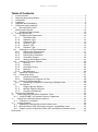
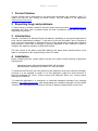
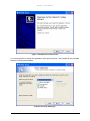
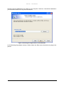
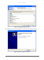
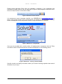
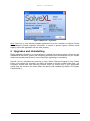
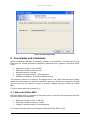
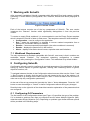
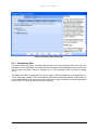
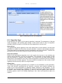
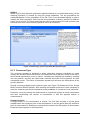
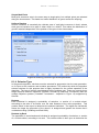
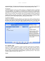
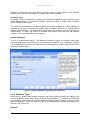
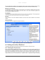
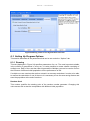
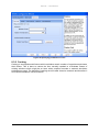
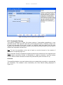
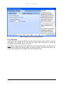
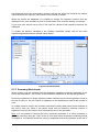
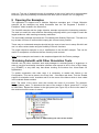
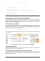
EXETER ADVANCED ANALYTICS LLP
User Manual
SolveXL – User Manual
Table of Contents
1
2
3
4
5
6
Current Version ..............................................................................................................3
Reporting bugs and problems .........................................................................................3
Introduction .....................................................................................................................3
Installation ......................................................................................................................3
Upgrades and Uninstalling ..............................................................................................8
Constraints and Limitations.............................................................................................9
6.1
Microsoft Office 2007 ..............................................................................................9
7
Working with SolveXL ...................................................................................................10
7.1
Workbook Requirements.......................................................................................10
8
Configuring SolveXL .....................................................................................................10
8.1
Configuring GA Parameters ..................................................................................10
8.1.1
Population Size .............................................................................................11
8.1.2
Algorithm Type ..............................................................................................12
8.1.3
Crossover Type .............................................................................................13
8.1.4
Selector Type ................................................................................................14
8.1.5
Mutator Type .................................................................................................15
8.1.6
Replacer Type ...............................................................................................16
8.2
Defining Link to Excel Worksheet ..........................................................................17
8.2.1
Defining the Chromosome .............................................................................17
8.2.2
Defining the Objectives .................................................................................18
8.2.3
Defining the Constraints ................................................................................19
8.2.4
Simulation Support ........................................................................................20
8.2.5
Writing Values Back to Excel .........................................................................21
8.3
Setting Up Program Options .................................................................................22
8.3.1
Running.........................................................................................................22
8.3.2
Caching .........................................................................................................23
8.3.3
Automatic Saving ..........................................................................................24
8.3.4
Backups ........................................................................................................25
8.3.5
Miscellaneous ...............................................................................................26
8.4
Advanced Configuration ........................................................................................27
8.5
Performing a Run ..................................................................................................27
8.5.1
Saving the Results ........................................................................................28
8.5.2
Displaying the Progress of a Run ..................................................................28
8.6
Resuming Suspended Run ...................................................................................29
8.6.1
Resuming Computation Comprising of Multiple Runs ....................................30
8.7
The Results...........................................................................................................30
8.7.1
Single Objective Results ...............................................................................30
8.7.2
Multiple Objective Results .............................................................................30
8.7.3
Summary Worksheets ...................................................................................31
9
Opening the Examples .................................................................................................32
10
Linking SolveXL with Other Simulation Tools ............................................................32
10.1 Using EPANET to Evaluate Fitness of Organisms ................................................33
11
Writing user defined Penalty multipliers ....................................................................34
11.1 Example of a multiplier ..........................................................................................34
12
Known problems .......................................................................................................34
12.1 Application crashing with access violation error ....................................................34
12.2 Microsoft Excel 2007 Worksheet running in compatibility mode ............................35
12.3 English version of Microsoft Office 2007 and different Windows locale .................35
References ...........................................................................................................................35
2
SolveXL – User Manual
1 Current Version
Version number can be determined in the About box accessible from SolveXL’s menu. To
make sure that you are running the latest version, visit the website of the application
(http://www.solvexl.com/).
2 Reporting bugs and problems
To report a bug or problem related to SolveXL please send an email to [email protected]
describing the issue and if possible attach an Excel Worksheet which can be used to
reproduce the problem.
3 Introduction
SolveXL is an add-in for Microsoft Excel that adds the possibility to use genetic algorithms to
solve various optimization problems. To be able to work with this add-in user is required to
have only basic knowledge of Microsoft Excel to enter appropriate formulas that represent
given problem. Some basic knowledge of genetic algorithms is also essential in order to
configure the algorithm properly to obtain best results.
The new version of the add-in uses Mark Morley’s GA library which should perform much
faster in comparison to the original library written in Pascal.
4 Installation
Before installing SolveXL, please make sure that your system meets following configuration
requirements:
Operating system: Microsoft Windows 2000, XP and Vista
Microsoft Excel: Microsoft Excel 2000, XP, 2003 and 2007
To install and use SolveXL the user performing this operation must have sufficient privileges.
Currently it is not possible to install or run this application under the limited account in
Microsoft Windows XP Home. Please ensure that Microsoft Excel isn’t running before
starting the installation.
To install the application it is necessary to download installation package from following
address: http://www.solvexl.com/. After downloading the installation package run the installer
“SolveXL.exe” and follow the instructions. SolveXL is always installed under current user.
3
SolveXL – User Manual
Figure 1 Installation welcome screen
It is recommended to install the application with typical options. This installs all the available
features including all examples.
Figure 2 Selecting Setup type
4
SolveXL – User Manual
SolveXL can be installed into any folder on your computer. However, it should be installed on
your hard drive and not on any removal devices.
Figure 3 Choosing the target folder to install SolveXL
In the following step please choose a folder where the Start menu shortcuts are going to be
placed.
5
SolveXL – User Manual
Figure 4 Choosing Start menu folder name
The installation will commence after pressing the “Install” button and should finish shortly.
Figure 5 Installation completed successfully
6
SolveXL – User Manual
Please launch Microsoft Excel after the installation completes. If the installation was
successful a toolbar similar to the one depicted on Figure 6 should appear in Microsoft Excel.
Click the “About” button on SolveXL's toolbar.
Figure 6 SolveXL disabled toolbar
It is necessary to send a hardware identifier (e.g. $5E2EE818) to [email protected] so
that a unique serial number can be generated for you based on this information. Click the
button as displayed on the next picture in order to copy the identifier to clipboard.
Figure 7 About box - unregistered
Once you are provided with a serial number (32 alphanumeric characters) click the "Enter
new serial number" button and paste the number as displayed on the following picture.
Figure 8 About box - entering a Serial Number
SolveXL should now display information about your license including expiration date and all
limitations of your copy.
7
SolveXL – User Manual
Figure 9 About box - registered
Note: Never try to copy already installed application from one computer to another! During
the installation process important information is stored in system registry. Without these
registry entries the application will not work properly.
5 Upgrades and Uninstalling
Before upgrading SolveXL it is not necessary to uninstall the previous version. Simply run the
installation of the newer version and everything should be done automatically for you. Please
make sure that Microsoft Excel is not running while upgrading or uninstalling
SolveXL can be uninstalled by removing it using “Add or Remove Programs” from Control
Panel or by clicking the “Uninstall” icon which is located in SolveXL’s folder under Start – All
Programs. Please note that removing SolveXL does not remove any of your documents
unless they are stored in the folder where the add-in was installed (by default “C:\Program
Files\SolveXL”).
8
SolveXL – User Manual
Figure 10 Removing SolveXL
6 Constraints and Limitations
When formulating a problem and deciding whether to use SolveXL it must be kept in mind
that there are certain restrictions imposed by Microsoft Excel (applies to Microsoft Excel
2003).





Maximum number of rows: 65,536
Maximum number of columns: 256
Number precision: 15 digits
Length of formula contents: 1,024 characters
Sheets in a workbook: limited by available memory
The maximum number of columns is the biggest issue. One might think that about putting
genes into rows instead of columns but when the results are saved every organism occupies
one row and thus the maximum number of decision variables (genes) is limited to around
250.
Full list of other limits can be found in [1].
6.1 Microsoft Office 2007
Microsoft Office 2007 is supported by the latest version of SolveXL and significantly extends
the limits applied to worksheets.



Maximum number of rows: 1,048,576
Maximum number of columns: 16,384
Length of formula contents: 8,192 characters
For further information about new features of Microsoft Excel 2007 see [2].
9
SolveXL – User Manual
7 Working with SolveXL
After successful installation SolveXL integrates within Microsoft Excel and creates a toolbar
containing 5 control buttons (Configuration, Run, Resume, Results and About) displayed in
Figure 11.
Figure 11 SolveXL Toolbar
Each of the buttons controls one of the key components of SolveXL. This new version
introduces the “Resume” function which significantly distinguishes it from the previous
version.
To create an empty Excel workbook it is recommended to use the Empty Project template
which is located in SolveXL’s folder in Start menu. This template creates an initial workbook.
 Configuration – used to configure the application
 Run – starts the optimization or attempts to recover crashed computation from a
backup file (if automatic backup is enabled)
 Resume – resumes suspended optimization (the active worksheet is resumed)
 Results – displays the pareto front in MO version
 About – displays information about license, expiration date and limitations
7.1 Workbook Requirements
The only requirement a workbook compatible with SolveXL must meet is that it contains one
worksheet named “Problem”. The worksheet containing configuration is created
automatically after pressing the “Configuration” button. This worksheet is by default hidden.
8 Configuring SolveXL
Configuration wizard is used to configure all required parameters of the application. It allows
setting up various options of genetic algorithm, defining cells containing values of genes,
objective functions, etc.
To navigate between the tabs in the Configuration wizard one can either use the “Next >” and
“< Back” buttons or directly click the name of the tab located at the top of the window. It is
recommended to go through all the tabs using the “Next >” button at least for the first time in
order not to skip any configuration parameters.
At the end of the set up process the (last tab) the “Next >” button disappears. Press the “OK”
button to save the settings or “Cancel” to leave Configuration without saving any changes.
Read the help on the right side of the wizard that contains explanation of the parameters that
are configured.
8.1 Configuring GA Parameters
The first screen of the Configuration wizard (see Figure 12) specifies the type of the problem.
If it is desired to optimize more than one objective function select Multiple Objective (MO),
otherwise select Single Objective (SO). Depending on problem type chosen different options
will be provided in the following steps.
10
SolveXL – User Manual
Figure 12 Selecting the problem type
8.1.1 Population Size
The second tab (see Figure 13) allows defining the size of the population GA works with. The
population size is important as it determines the diversity of the population at the start of the
run and also how long it takes to complete a run. The population size must be an integer
value.
The higher the value of population size is the longer it takes the algorithm to complete its run.
This is especially problem of the Generational, Generational Elitist and NSGA II algorithms. It
is recommended to enter value lower than 1000 as it might be difficult to stop the algorithm
using “Stop” or “Pause” buttons on slower machines.
11
SolveXL – User Manual
Figure 13 Defining the size of the population
8.1.2 Algorithm Type
In the third tab (see Figure 14) the genetic algorithm is selected. The appearance of the tab
varies according to the problem type settings. In MO version there is only one algorithm
available (NSGA II) however in SO there are three algorithms to choose from.
Generational
The generational genetic algorithm is the most widely-used. At each iteration, an entire new
population is created from the old by using the selection, crossover and mutation operators.
This means that a new population must be evaluated for each new population. Therefore the
generational GA can be more effective but also more time-consuming.
Generational Elitist
Similar to the generational algorithm, but in this version the top one or two solutions are
copied, without alteration, into the next population. The remainder of the population is filled
with the products of crossover and mutation. This ensures that the best solution(s) are
retained from one population to the next. When this algorithm is selected a text box enabling
to define the level of elitism appears. The level of elitism corresponds to the number of best
organisms that are directly copied to next generation.
Steady State
The steady-state algorithm generates only a handful of new individuals in each generation.
These new solutions, generated by the selection, crossover and mutation operators are
added to the current population by replacing weaker solutions in the population. To use
steady-state, an extra operator (a Replacer) is needed to determine which weaker solutions
to replace. When Steady state algorithm is used an extra tab appears (see Figure 18
Choosing replacer used in SO Steady StateFigure 18) to allow user specify the type of a
replacer.
12
SolveXL – User Manual
NSGA II
NSGA-II [4] is multi-objective optimization algorithm based on non-dominated sorting. At first
offspring population is created by using the parent population. The two populations are
combined together to form population of size 2N. Then a non-dominated sorting is used to
classify the entire population. After that the new population is filled by solutions of different
fronts, one at a time. The filling starts with the best non-dominated front and continues with
solutions form other fronts until the population size of N is reached.
Figure 14 Choosing a genetic algorithm (MO problem type)
8.1.3 Crossover Type
The crossover operator is designed to share information between individuals to create
entirely new solutions which have some of the attributes of their parents, similar to the way in
which sexual reproduction occurs in nature. Normally two offspring are created by crossing
over two parents, and they are often better solutions that either of their parents, but also
occasionally worse. The choice of crossover operator can influence the effectiveness of the
genetic algorithm.
SolveXL currently supports three crossover types (see Figure 15) Simple One Point, Simple
Multi Point and Uniform Random. After selecting the desired crossover it is also necessary to
enter the crossover rate which corresponds to the probability of a crossover to be performed.
Crossover occurs by splicing the chromosome at a particular point(s) on each chromosome
and then recombining one section of chromosome A with the opposite section of
chromosome B.
Simple One Point
A single location in the chromosome is chosen. The first child consists of all the genes
located before this crossover point of the chromosome A, and the genes after this crossover
point of chromosome B. Similarly the second child consists of the first portion of chromosome
B and the second portion of chromosome B.
13
SolveXL – User Manual
Simple Multi Point
Multi-point crossover acts in the same way as single-point, but multiple points are selected
along the chromosome. This leads to a better distribution of genes across the offspring.
Uniform Random
Uniform crossover is essentially the ultimate case of multi-point crossover in that it selects
each gene at random to be part of either child A or child B. This makes the distribution of
genetic material independent of the position of the gene in the chromosome.
Figure 15 Choosing crossover type and its parameters
8.1.4 Selector Type
In the genetic algorithm, solutions must be selected for progression into the next generation,
or for input to the crossover and mutation procedures. The method by which the algorithm
selects solutions for this purpose then is highly important for the correct operation of the
algorithm. The type of selector used depends on the problem type. There are currently three
single objective selection operators (Roulette, Roulette by Rank and Tournament) and one
multiple objective operator (Crowded Tournament – depicted in Figure 16) supported by
SolveXL.
Roulette
Each individual is assigned a probability of selection, or section of a roulette wheel,
according to the ratio of its fitness over the total fitnesses of the entire population. This
roulette wheel is then spun to determine the selected individual. The higher the individual's
fitness the larger the proportion of the wheel it is assigned and greater the chance that it
undertakes mating (Goldberg and Deb 1990).
Roulette by Rank
The population is sorted and each individual is assigned a probability of selection, or section
of a roulette wheel, according to its rank. This roulette wheel is then spun to determine the
14
SolveXL – User Manual
selected individual. The higher the individual's rank the larger the proportion of the wheel it is
assigned and greater the chance that it undertakes mating (Goldberg and Deb 1990).
Tournament
Tournament selection involves the random selection of a designated number of individuals
from the population, who compete in a tournament for inclusion into the mating pool.
Tournament selection, in its simplest form consists of a binary tournament involving the direct
competition of two individuals for survival by the comparison of their fitness function, with the
fitter of the two surviving. The tournament size can be increased, thereby increasing the
selection pressure in the GA. This ranking of the population allows for a constant selection
pressure (as in rank based fitness allocation). Use of tournament selection has shown better
performance than the roulette wheel selection (Goldberg and Deb 1990).
Crowded Tournament
Similar to the standard Tournament Selection, two solutions are chosen at random from the
population and compared. The solution with better (lower) rank wins. If both solutions have
the same rank then the solution with larger crowding distance wins. In case that both
solutions have the same rank and also crowding distance then winner is chosen randomly.
Figure 16 Choosing GA selector
8.1.5 Mutator Type
The mutation operator is designed to provide new genetic material during an optimisation.
Without the mutation operator, the algorithm could find locally optimal solutions without
searching for better globally optimal solutions. The mutation operator works by selecting a
gene at random in a chromosome and changing it to a random value (within the bounds of
the gene). This is performed within a certain probability, specified by the user. There are two
mutators available in SolveXL (see Figure 17).
Simple
15
SolveXL – User Manual
Mutation is performed on a gene when a random value is bigger than the user selected
mutation rate. This gene will be given a random value within its range.
Simple by Gene
An integer value is calculated by multiplying the mutation probability times the chromosome
length (MutationRate * Chormosome.Length). When this value is smaller then a random
value, mutation is performed.
The value of the probability of mutation needs to be carefully thought out. If the probability of
mutation is less than 1/(chromosome length) then no mutation will occur. If 1/(chromosome
length) ≤ MutationRate < 2/(chromosome length) then one mutation can be expected per
chromosome. In effect, the choice of mutation rate implies how many bits will undergo
mutation. (The Ammended Morley GA Library)
Adaptive Mutation
This is an experimental feature. The algorithm records a history of mutations and tracks
mutations that lead to improvement of the fitness of the organism. Use of adaptive mutation
can increase the performance of GA however the learning time is rather long and should be
thousands of generations.
Figure 17 Choosing Mutator and defining its parameters
8.1.6 Replacer Type
When using a Steady State genetic algorithm, the new solutions created are added to the
current population rather than creating a whole new population. To maintain the population
size therefore, some solutions must be replaced. Deciding which solutions to replace is the
job of the Replacer. There are number of criteria for deciding which solutions are replaced in
SolveXL (see Figure 18):
Weakest
16
SolveXL – User Manual
The new individual is added to the population which is then sorted according to fitness. The
solution with the worst fitness is then deleted (note that this could be the new solution).
Weakest (unconditional)
The population is sorted according to fitness before new individual is added and the solution
with the worst fitness is then deleted (note that unlike in the case of Weakest replacer the
new individual is added every time).
First Weaker
This starts with the best individual and works its way down the population. The first solution it
encounters with worse fitness than the new solution is replaced.
By Rank
This is similar to the First Weaker method, but uses rank values instead of raw fitness
values.
Uniform Random
The solution which is replaced is selected randomly.
Figure 18 Choosing replacer used in SO Steady State
8.2 Defining Link to Excel Worksheet
This section describes all the options that can be set under the “Excel Link” tab.
8.2.1 Defining the Chromosome
Each of the decision variables for a problem constitutes a gene in the genetic algorithm. All
of the genes are appended together to form a chromosome. Therefore the choice of genes
determines what variables the genetic algorithm uses to discover optimal solutions. Microsoft
Excel cells corresponding to the genes must occupy continuous area (range). Type in the
range address (e.g. A1:C5) and press the “Update” button to populate the grid containing
17
SolveXL – User Manual
parameters of genes. Please note that the after the pressing the “Update” button the values
of existing cells are preserved and new cells are filled in with default values.
Hint: To set the value of a whole column, click on its heading with right mouse button and
choose or type in the desired value.
Figure 19 Defining the chromosome
Hybrid Integer Bounded Gene
The gene is an integer number (e.g. 1, 23, 456) and its value is within the range [upper
bound, lower bound]
Hybrid Real Bounded Gene
The gene is a real number (e.g. 1.2, 3.45) and its value is within the range [upper bound,
lower bound]. The precision of real gene is defined in Options - Miscellaneous tab.
Hybrid Gray Integer / Real Bounded Gene and
These are special cases of the two previously stated gene types used especially in
optimization of water networks. These gene types should be used with pipe-sizing problems.
8.2.2 Defining the Objectives
Exactly one objective must be specified in Single objective version or at least two objectives
in multiple objective version. Objectives must occupy continuous range of cells. Type in the
address of the range (e.g. A1:C5) and press the “Update” button to populate the grid
containing parameters of objectives.
Each objective is described by address of an Excel cell, the function that is applied to it and
its name. Objective function can be either minimize or maximize.
Hint: To set the value of a whole column, click on its heading with right mouse button and
choose or type in the desired value.
18
SolveXL – User Manual
Figure 20 Defining objective functions
8.2.3 Defining the Constraints
Constraints are used when it is wanted to penalise certain variables for going out of the
bounds. For instance in a multiple objective problem, if one of the objectives is the cost of a
solution and the budget is only £2M, then solutions outside of this are useless and should be
discouraged.
Constraints in SolveXL are handled by Excel. It is users’ responsibility to write the formulas.
To enable use of constraints tick the corresponding checkbox and enter address of an Excel
cell which contains penalty cost (SO) or infeasibility (MO) of given solution (see Figure 21).
Example of a Constraint
The value of objective function must not exceed 50. Let us assume that the objective function
is stored in cell C5. The value of the penalty cell might look similar to this:
=IF(C5>50,(C5-50)*1000,0)
The above formula penalises all solutions violating given constraint.
19
SolveXL – User Manual
Figure 21 Defining the constraints or infeasibility
8.2.4 Simulation Support
Simulation allows linking SolveXL with other simulation packages used to evaluate fitness of
solutions. To enable this feature tick the appropriate checkbox on this tab and enter the
name of VB macro to be called to evaluate fitness of an organism (see Figure 22). For more
details refer to chapter 10 (page 32).
Please note that automatic re-calculation of the worksheet is disabled while GA computation
is running. It is the responsibility of user defined macro to ensure that worksheet is
recalculated at the end of the evaluation (if this is necessary).
20
SolveXL – User Manual
Figure 22 Setting up SolveXL to work with other simulation packages
To verify that a macro of the specified name can be executed by SolveXL please press the
“Test” button to attempt to execute it.
8.2.5 Writing Values Back to Excel
This feature (displayed in Figure 23) allows writing current generation and run back into
specified Excel cells. This might be used to implement user defined penalty multipliers that
take into account progress of the algorithm.
21
SolveXL – User Manual
Figure 23 Writing values of run & generation into Excel
8.3 Setting Up Program Options
This section describes all the parameters that can be set under the “Options” tab.
8.3.1 Running
This tab (displayed in Figure 24) specifies parameters of a run. The most important variable
is the number of generations in every run. It is also possible to create a batch consisting of
multiple runs. Each of the runs then lasts N generations. Multiple runs can be used to find out
the influence of different initial populations on the performance of GA.
If multiple runs are used results are then stored in a summary worksheet. In order to be able
to resume the calculation of one of the runs it is necessary to use the auto saving feature and
save the population at the end of each run.
Random Seed
This number modifies the starting point of the random number generator. Changing this
value causes GA to start the computation with different initial population.
22
SolveXL – User Manual
Figure 24 Specifying parameters of runs
8.3.2 Caching
Caching is an experimental feature which maintains certain number of organisms and stores
their fitness. This is done to reduce the time normally needed to re-evaluate fitness of
existing solutions which might be an issue when complex formulas or external simulation
packages are used. The benefits of caching are still under intensive research and therefore it
is not recommended to use this feature.
23
SolveXL – User Manual
Figure 25 Using cache to improve the performance
8.3.3 Automatic Saving
This feature (displayed in Figure 26) allows saving of intermediate populations in user
specified interval. This might be useful when performing optimization containing multiple runs
to save the population at the end of each run. Without using this option only the best
organism (SO) or pareto front (MO) is saved to summary result sheet which does not allow to
resume the computation at later time.
Hint: To save the population at the end of each run set the interval to the number of
generations comprising single run.
Note: Automatic saving of population negatively affects the performance of the algorithm and
might produce enormous number of worksheets! It might be desired to use the backup
function which is faster and does not create any worksheets (refer to section 8.3.4).
Overwrite
This specifies whether new result sheets which are created either manually or automatically
are overwritten. This variable is also controlled by the Save Results dialog (displayed in
Figure 31).
24
SolveXL – User Manual
Figure 26 Automatic saving of the population
8.3.4 Backups
This function allows storing population and other information that can be used to recover the
computation into external file. In case that the addin crashes and Excel is closed the
computation can be restored later from the file.
Note: Backup negatively affects the performance of the algorithm however the impact is not
as significant as when auto saving is used. The backup interval should be chosen wisely with
respect to the character of the problem and assumed duration time.
25
SolveXL – User Manual
Figure 27 Backup of population into an external file
Recovery after a crash
To recover the information saved using the backup function. Just press the “Run” button. If
any backup was created it is inspected and in case that it contains any information a new
worksheet is created containing the whole population from the last backup before a crash
occurred.
Figure 28 A message box displayed when restoring population from a backup file
8.3.5 Miscellaneous
This is the last tab of the configuration wizard. It allows user to define several options but
also to enter new serial number in order to extend the expiry date of the application. Please
contact the author if your version of SolveXL has expired and you would like to continue
using it.
Float Precision
The value of this variable controls the precision of Real Bounded Genes (if they are utilised).
The default value is 4 however the precision can be increased up to 8.
Chart Update Interval
26
SolveXL – User Manual
This variable specifies the update interval of the chart and grid displaying the progress of GA
during a run. Please
Display Progress Chart
The state of this variable indicates whether progress chart will be displayed during the
computation. In case that the application is crashing unexpectedly, try to disable the progress
chart.
Note: Updating the chart is a time consuming operation which can significantly decrease the
performance of the application. It is recommended to disable updating of a chart and grid
when working with population sizes greater than 1000.
Figure 29 Miscellaneous options
8.4 Advanced Configuration
The previous version of SolveXL was exposing a worksheet called “Settings” which
contained all the configuration parameters. In the current version this worksheet is hidden by
default however it is possible to unhide it. To do so open your workbook and go to “Format >
Sheet > Unhide...” and select the Settings sheet.
Note: Please be careful when editing the settings directly because the values read from this
sheet are not validated against any errors.
8.5 Performing a Run
After configuring all the parameters the algorithm can be executed by pressing the Run
button in application’s toolbar.
27
SolveXL – User Manual
Figure 30 Starting the optimization
8.5.1 Saving the Results
Before the computation process starts a pop up window appears requiring to enter a name of
worksheet into which results will be saved at the end of computation.
Note: Bear in mind that maximum length of the name of a worksheet is limited to 30
characters.
Figure 31 The Save Results Form
It is possible to choose a name of existing worksheet with results by clicking the down arrow
on the right side of the edit box. Please note that the “Overwrite data” checkbox must be
ticked when entering the name of an existing worksheet.
The algorithm can be started by pressing the “OK” button or the run can be aborted using the
“Cancel” button.
8.5.2 Displaying the Progress of a Run
When the algorithm is running it displays some variables reflecting its progress (see Figure
32). The overall progress of the algorithm is displayed on the progress bar. According to the
value of the “Chart Update Interval” which can be set on the “Options > Miscellaneous” tab
(see Figure 29). The algorithm displays the obtained solutions in form of a grid containing
values of genes, objective functions, penalty / infeasibility and other statistical indicators. To
visualise the progress a chart is used to display the best pareto front in MO or just the fitness
of the best organism in SO.
28
SolveXL – User Manual
Disable the chart
Figure 32 Form showing the progress of the algorithm
The chart can be disabled or enabled by clicking at the minimise arrow as depicted on Figure
32. Disabling the chart might be especially useful when the application crashes regularly at
the same phase of computation.
Note: Setting too low value of chart update interval negatively affects the performance of the
algorithm because chart and grid updating is a time consuming operation. In case of MO run
it is possible to select the objectives that are displayed on the chart. This can be done using
the combo boxes corresponding to the X & Y axes in the “Chart Options” panel (the chart is
not updated immediately after changing these values).
8.6 Resuming Suspended Run
To resume a run which was stopped using the “Stop” button or any save point created using
the auto save feature. It is necessary to select appropriate worksheet containing the
population and press the “Resume” button.
In order to be able to resume the GA the population size, number of genes and objectives
must not be changed. Other parameters such as number of runs, generations or GA settings
can be modified. Please bear in mind that changing GA settings might lead to unwanted
effects.
29
SolveXL – User Manual
Note: If the computation has reached the maximum number of generations then the
application displays an error and does not allow resuming of the run. There are several ways
how to bypass this. The easiest way is to increase the number of generations in the
Configuration wizard (refer to section 8.3.1 on page 22).
8.6.1 Resuming Computation Comprising of Multiple Runs
When resuming the results that were obtained from multiple runs then the algorithm normally
completes current run and continues on consequent runs. This behaviour might not be
wanted in certain situations. One might use multiple runs to see the effect of different initial
populations and then just continue the computation with the best results obtained so far.
In order to do this it is necessary to change the configuration of the GA and also to modify
the worksheet containing the results. In the configuration the number of runs must be set
back to 0 and the number of generations increased to a desired value. Then the worksheet
with results has to be changed. Find the value indicating the Run (highlighted in Figure 33)
and ensure that it is set to 0.
Figure 33 Resetting the number of a run to 0
8.7 The Results
After completing a run (either reaching the given number of generations or terminating it
using the “Stop” button) the obtained results are saved to the worksheet which was selected
prior to starting the GA.
8.7.1 Single Objective Results
After SO algorithm finishes it updates the “Problem” worksheet with gene values of the best
organism found and generates a worksheet containing the whole population and the global
best organism stored at the end. The global best organism is used by the GA library to store
the best organism from multiple runs and necessarily does not have to be the best organism.
The organisms are sorted according to fitness function thus the best organism can always be
found on the top of the table.
Note: When using Generational algorithm the organism which is written into the “Problem”
sheet does not need to exist in the results worksheet containing the population. This is due to
the character of Generational algorithm which unlike the Elitist version of this algorithm does
not guarantee that any of the fittest organisms propagates to the next generation.
8.7.2 Multiple Objective Results
Results in MO version are represented by the Pareto Front and are stored in the Results
sheet of the Workbook (Please note that the whole population is stored in the worksheet and
that the best pareto front is formed only by organisms with rank equal to 0. The true pareto
front can be easily obtained using Excel’s automatic filter which can be found under “Data >
Filter > Automatic Filter”). To display the results in a form of a chart similar to the one that
30
SolveXL – User Manual
was displayed during the computation process, activate the sheet that contains the desired
values and click the “Results” icon located in the SolveXL’s toolbar.
When the results are displayed it is possible to change the objective functions that are
displayed in the chart and also to zoom to certain parts of the chart by drawing a rectangle.
If you move your mouse over a point in the chart the values of both objective functions are
displayed.
To update the decision variables in the Problem worksheet please click on the point
representing desired solution with left mouse button.
Figure 34 Results Browser
8.7.3 Summary Worksheets
When multiple runs are selected then the application generates summary worksheet at the
end of the computation. The content of the worksheet is different for SO and MO problems.
Summary worksheet of a single objective problem contains only the best organisms found at
the end of each run. So, the number of organisms on the worksheet is equal to the number of
runs.
In multiple objective version the summary worksheet contains best pareto fronts obtained at
the end of each run. Each of the pareto fronts can be formed by different number of
organisms however the number never exceeds the size of the population.
Note: It is not possible to resume GA from a summary worksheet. It is either necessary to
abort the execution using the “Stop” button (in this case normal worksheet containing results
is created) or to enable the automatic saving of population and save population at the end of
31
SolveXL – User Manual
each run. The use of automatic saving of population at the end of each run is recommended
because it gives the possibility to resume the GA later (refer to section 8.3.3 on page 24).
9 Opening the Examples
The application is shipped with 2 Multiple Objective examples and 1 Single Objective
example. All the examples are easily accessible from the “All Programs > SolveXL >
Examples” folder located in the Start menu.
The first MO example and the single objective example represent the Advertising selection.
The task is to select the most effective advertising campaign within your budget to reach the
largest audience, while meeting necessary restrictions.
The second MO example represents the “Purchasing with Quantity Discounts”. The task is to
buy at least 155 litres of solvent while keeping the cost as low as possible.
These easy to understand examples should help the user to learn how to setup SolveXL and
use it to solve various tasks using the flexibility of Excel’s functions.
The single objective example is only a modification of the first MO example. This can be
useful for comparison of solutions that are found by both versions.
Note: All the examples are based on the samples shipped with the Evolver package.
10 Linking SolveXL with Other Simulation Tools
SolveXL can use other simulation tools and packages to evaluate fitness of organisms. In
order to use this functionality simulation software must expose its API in form of DLL library
(e.g. EPANET) or any other way that allows invoking its functions from Visual Basic for
Applications.
To enable cooperation with other tools it is necessary to enable this feature in the
Configuration. This can be done in the Excel Link – Simulation tab sheet. Tick the “Enable
support for simulation tools” checkbox and fill in the name of the Macro which is then called
in the evaluate fitness method.
Note: The name of the macro must also contain the name of its module. For example:
Module1.Macro_name. To determine the name of the module in Excel, press Alt+F11 to get
to VBA Editor. Expand the folders in the right panel (see Figure 35) to find out the name of
the module where the macro is stored.
Figure 35 A panel in VBA showing the name of the module
32
SolveXL – User Manual
10.1 Using EPANET to Evaluate Fitness of Organisms
The easiest way how to run simulations with EPANET is to modify one of the examples
shipped with SolveXL.
The example code in VB comprises of two modules (EPANetDLL and EPANetInterface)
 EPANetDLL is module which was imported into the project. The original file
epanet2.bas is part of the epanet toolkit (EN2toolkit.zip) which can be downloaded
from EPANet website [3]. To insert this module into an existing workbook press
Alt+F11 to get to the VBA editor, right-click the Modules folder and choose “Import
file...”

EPANetInterface is a set of functions exploiting the EPANet interface created to
simplify calling of original methods. The key functions are:
o
o
o
o
openNetwork – opens the EPANET input file and initializes hydraulic solver
closeNetwork – shuts down the EPANET and closes all files
solve – runs the hydraulic simulation of the network
simulation – main function which writes new pipe diameters to EPANET, runs
hydraulic simulation and then reads node heads from EPANET and stores
them in the Excel worksheet.
Public Sub openNetwork()
ERROR = ENOpen("input_file.inp", "report_file.rep", "")
ERROR = ENopenH()
End Sub
Public Sub closeNetwork()
ERROR = ENclose()
End Sub
Public Sub solve()
'this function is based on example contained in EPANET help
Dim t As Long
Dim tstep As Long
'there must be 10 in ENinitH otherwise the simulation results would be
incorrect
ENinitH (10)
Do
ENrunH (t)
ENnextH (tstep)
Loop While (tstep > 0)
End Sub
Sub simulation()
Dim i, j As Long
ActiveSheet.Calculate
'write new diameters to EPANet
For i = 1 To selectedLinkCount
Call
EPANetInterface.setLinkDiameter(linkIndexAddr.Cells(i,
diamAddr.Cells(i, 1).value)
Next i
1),
33
SolveXL – User Manual
'run simulation
EPANetInterface.solve
'read head values and store them to internal variables
For j = 1 To nodeCount
nodeAddr.Cells(j, 1).value = EPANetInterface.getNodeHead(j)
Next j
'recalculate the worksheet (otherwise cost and penalty wouldn’t change)
ActiveSheet.Calculate
End Sub
11 Writing user defined Penalty multipliers
Penalty multipliers can be used to modify the penalty function according to the progress of
the GA. To use penalty multipliers it is necessary to get the current generation and run from
the GA. This can be achieved by enabling the “write back” feature in Excel Link – Write Back
tab (see the section 8.2.5 on page 21).
11.1 Example of a multiplier
This example demonstrates creation of a simple penalty multiplier which changes its value
every run after 100 generations. Let us assume that value of generation is written into cell B2
and current run is stored in cell B1. The penalty function which is defines the constraint is
stored in cell B7 and contains following formula:
=(some function)*B5
The actual value of the penalty multiplier is stored in cell B5. A screenshot of the worksheet
is in Figure 36.
Figure 36 Example of creation of user defined penalty multiplier
12 Known problems
This chapter highlights some of the known problems related to SolveXL and provides the
user with possible solutions (where applicable).
12.1 Application crashing with access violation error
This problem is related to the TChart component which is used to display the progress chart
during the run. The only known workaround is to hide the progress chart to prevent it from
updating and thus crashing.
34
SolveXL – User Manual
12.2 Microsoft Excel 2007 Worksheet running in compatibility mode
Please note that when Microsoft Excel 2007 opens a workbook created using an older
version the workbook is opened in compatibility mode. This implies that the limits of ranges in
Excel remain the same as in the previous version and might cause problems when working
with larger worksheets (over 255 columns or over 65535 rows). In order to resolve this
problem, please save the worksheet in new format.
12.3 English version of Microsoft Office 2007 and different Windows
locale
Microsoft Excel 2007 contains a bug which causes SolveXL not to be able to operate if the
language version of Microsoft Office does not match the locale used in Microsoft Windows.
The only workaround at the moment is to change the locale in Windows to match the
language version of Microsoft Office or maybe to download Multilanguage pack for Microsoft
Office.
Further
information
about
this
bug
can
be
found
at:
http://support.microsoft.com/kb/320369.
References
1. Microsoft Excel 2003 Limits
http://office.microsoft.com/en-gb/excel/HP051992911033.aspx
2. Microsoft Excel 2007 Limits
http://blogs.msdn.com/excel/archive/2005/09/26/474258.aspx
3. EPANet Project
http://www.epa.gov/nrmrl/wswrd/epanet.html
4. Deb, K., S. Agrawal, et al. (2000). A Fast Elitist Non-Dominated Sorting
Genetic Algorithm for Multi-Objective Optimization: NSGA-II. Kanpur, India,
Indian Institute of Technology, Kanpur Genetic Algorithms Laboratory.
Microsoft, Excel, Office, XP, Vista and Windows are either registered trademarks or
trademarks of Microsoft Corporation in the United States and/or other countries.
35