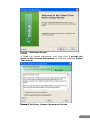
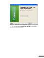
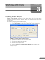
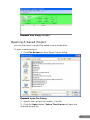
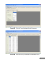
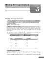
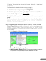
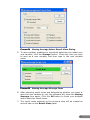
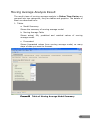
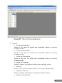
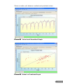
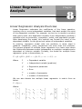
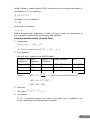
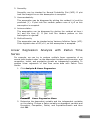
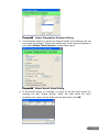
1
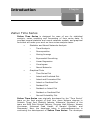
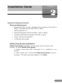
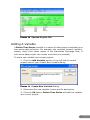
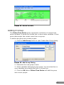
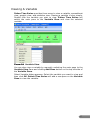
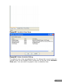
User Manual Content Chapter 1 Introduction 2 Zaitun Time Series 2 Chapter 2 Installation Guide 4 System Requirements 4 Zaitun Time Series Installation 4 Chapter 3 Working with Data 9 Creating A New Project 9 Opening A Saved Project 10 Adding A Variable 11 Adding A Group 12 Editing A Variable/Group 13 Duplicating A Variable/Group 14 Deleting A Variable/Group 16 Viewing A Variable 17 Viewing A Group 22 Transforming A Variable 23 Exporting The Data 24 Importing The Data 25 Adding A Stock Market Data 29 Viewing A Stock Market Data 30 Importing Live Stock Market Data 31 Chapter 4 Trend Analysis 34 Trend Analysis Overview 34 Trend Analysis with Zaitun Time Series 35 Trend Analysis Result 37 Chapter 5 Moving Average Analysis 40 Moving Average Overview 40 Moving Average with Zaitun Time Series 41 Moving Average Analysis Result 44 Chapter 6 Exponential Smoothing Analysis 47 Exponential Smoothing Overview 47 Exponential Smoothing Analysis with Zaitun Time Series 51 Exponential Smoothing Analysis Result 54 Chapter 7 Decomposition Analysis 57 Decomposition Analysis Overview 57 Decomposition Analysis with Zaitun Time Series 57 Decomposition Analysis Result 60 Chapter 8 Linear Regression Analysis 63 Linear Regression Analysis Overview 63 Linear Regression Analysis with Zaitun Time Series 66 Linear Regression Analysis Result 68 Chapter 9 Correlogram 72 Correlogram Overview 72 Correlogram with Zaitun Time Series 73 Correlogram Result View 75 Chapter 10 Neural Network Analysis 77 Neural Network Overview 77 Neural Network Analysis with Zaitun Time Series 78 Neural Network Modeling Result 82 Zaitun Time Series User Manual Zaitun Software Developer Team www.zaitunsoftware.com Chapter Introduction 1 Zaitun Time Series Zaitun Time Series is designed for ease of use for statistical analysis, series modeling and forecasting of time series data. It provides several statistics and neural networks models, and graphical tools that will make your work on time series analysis easier. • • Statistics and Neural Networks Analysis o Trend Analysis o Decomposition o Moving Average o Exponential Smoothing o Linear Regression o Correlogram o Neural Networks Graphical Tools o Time Series Plot o Actual and Predicted Plot o Actual and Forecasted Plot o Actual vs Predicted Plot o Residual Plot o Residual vs Actual Plot o Residual vs Predicted Plot o Normal Probability Plot Zaitun Time Series was originally developed by the “Time Series” team as the final project of their four years diploma degrees in Sekolah Tinggi Ilmu Statistik Jakarta, Indonesia. Members of the team are Rizal Zaini Ahmad Fathony, Suryono Hadi Wibowo, Wawan Kurniawan, Muhamad Fuad Hasan, Al Maratul Sholihah, and Rismawaty. Now, the developer team in zaitunsoftware.com is continuing the development of Zaitun Time Series. The developer 2 team now consists of four members who work hardly in developing Zaitun Time Seiries. The members of the team are: Rizal Zaini Ahmad Fathony, the founder and core programmer of Zaitun Time Series, Suryono Hadi Wibowo as programmer and GUI designer, Khaerul Anas as programmer, and Lia Amelia as documentation and administrator of Zaitun Time Series website. Zaitun Time Series is freeware. It can be used for any purpose, including commercial use. This software is provided "as is" without warranty of any kind, either expressed or implied. Zaitun Time Series copyright © 2007-2010 zaitunsoftware.com. All Rights Reserved. 3 Installation Guide Chapter 2 System Requirements Minimum Requirements • Windows XP (SP2 or later), Windows Vista, Windows 2000 (SP4 or later), or Windows Server 2003 (SP1 or later) • .NET Framework 2.0 • 600 MHz processor (Recommended: 1 GHz or faster) • 192 MB of RAM (Recommended: 256 MB or more) • 1024 x 768 screen resolution • 10 MB hard drive space Zaitun Time Series Installation Zaitun Time Series installation is very simple and only takes a few minutes. To install Zaitun Time Series: 1. Please ensure that .NET Framework 2.0 is installed in your system. 2. Start “zaitun.msi”. It will install Zaitun Time Series into your computer. The welcome screen appears. Click Next. 4 Figure 1 Welcome Screen 3. Read the license agreement, and then click I accept the terms in the License Agreement to continue installing Zaitun Time Series. Figure 2 End-User License Agreement Screen 5 4. Choose Destination Location Screen appears. You can choose to install Zaitun Time Series into the default directory “C:\Program Files\Zaitun Time Series” or choose another directory. If you want to change the destination location of Zaitun Time Series, click Browse button. Click Next button to install into default directory. Figure 3 Choose Destination Location Screen 5. Ready to Install Screen appears. Click Install to begin the installation. 6 Figure 4 Ready to Install Screen Figure 5 Installing Zaitun Time Series Screen 6. After the installation is complete, setup will inform you that the installation is successful. You may then launch Zaitun Time Series by clicking on “Launch Zaitun Time Series” check box. Click Next to continue and finish the setup. 7 Figure 6 Installation Completed Screen 7. You can start using Zaitun Time Series by clicking the shortcut on start menu items. 8 Working with Data Chapter 3 Creating A New Project Zaitun Time Series represents time series data with the data point frequency (annual, monthly, weekly, daily, etc) ranging from start date to end date. To create a new time series data project: 1. Click File New to open the Create New Project dialog box. Figure 7 Create New Project Dialog 2. Specify the frequency of time series data. 3. Set the start date and end date. 4. Set the new project name. 5. Click the OK button. Zaitun Time Series will create a new empty project. 9 Figure 8 New Empty Project Opening A Saved Project You can also open a project file saved in your media disk. To open a saved project: 1. Click File Open to show Open Project dialog. Figure 9 Open File Dialog 2. Specify your project file location (.zft file) 3. Click the Open button. Zaitun Time Series will open the selected project file. 10 Figure 10 Opened Project File Adding A Variable A Zaitun Time Series variable is a series of data points constituting one time series data collection. For example, the recorded (annual, monthly, weekly, daily) time series values of the Indonesian Exchange Rate. A time series data project can contain more than one variable. To add a new variable into current project: 1. Click the Add Variable button on top left side of current project view to open Create New Variable dialog. Figure 11 Create New Variable Dialog 2. Determine the new variable’s name and its description. 3. Click the OK button. Zaitun Time Series will add this variable into current project. 11 Figure 12 Added Variable Adding A Group The Zaitun Time Series group represents a collection of several time series variables. A group can contain two or more series variables. A time series data project can contain more than one group. To add a new group into current project: 1. Click the Add Group button to open Create New Group dialog. Figure 13 Add Group Dialog 2. Determine the new group’s name. 3. Select variables belonging to this group. You can select two or more variables by pressing the Shift or Control key. 4. Click the OK button. Zaitun Time Series will add this group into current project. 12 Figure 14 Added Group Editing A Variable/Group You can edit the name or description of a variable/group. To edit a variable/group: 1. Select the variable/group to be edited. Figure 15 Selected Variable 2. Click the Edit button to show the Edit dialog. Figure 16 Edit Variable Dialog 13 3. Edit the name or description of this variable, and then click the OK button. Figure 17 Edited Variable Duplicating A Variable/Group You can duplicate a variable/group. A duplicated variable/group has the same value as its source. To duplicate a variable/group: 1. Select the variable/group you want to duplicate. Figure 18 Selected Variable 2. Click the Duplicate button to show the Duplicate dialog. 14 Figure 19 Duplicate Variable Dialog 3. Enter the new variable/group’s name and then click the OK button. Zaitun Time Series will create a new variable/group that has same value as the source variable/group. Figure 20 Data View Screen after Duplicating the Variable Deleting A Variable/Group You can also delete a variable/group you have created. To delete a variable/group: 1. Select the variable/group you want to delete. 15 Figure 21 Selected Variable 2. Click the Delete button. A confirmation dialog appears. Click Yes if you are sure you wish to delete the selected variable/group. Figure 22 Confirmation Dialog 3. If you click Yes on the confirmation dialog, then the selected variable/group will be deleted from the current project. Figure 23 Data View Screen after Deleting a Variable 16 Viewing A Variable Zaitun Time Series provides three ways to view a variable, spreadsheet view, graphic view, and statistics view. Viewing a variable is very simple. Double click the variable you wish to view. Zaitun Time Series will switch the main pane to the Variable View and view the selected variable. Figure 24 Variable View You can also view a variable by manually switching the main pane to the Variable View Pane and clicking Add Pane button on the top left side of the Variable Pane. Select Variable dialog appears. Select the variable you want to view and then click OK. Zaitun Time Series will add a new pane on the Variable Pane to view the variable. 17 Figure 25 Variable View Pane Figure 26 Select Variable Dialog The default view is the spreadsheet view. To change the current view of a variable click on the Variable View Combo Box on the top of the Variable View pane. You can switch to graphic view or statistics view. 18 Figure Figure 27 Spreadsheet View Spreadsheet View shows variable values on a grid, it makes it easy for you to input or edit variable values by pressing numeric keys directly from keyboard. You can also paste values from an external program like Excel by right clicking the grid and selecting Paste menu. Figure 28 Pasting Data into Spreadsheet View Graphic View shows variable values on a line chart. It makes it easy for you to analyze graphically the components of time series data of a variable. You will soon know whether the variable contains trend, cyclic, seasonal and irregular component. 19 Figure 29 Graphic View Statistics View shows simple descriptive statistics of a variable making it easy for you to analyze statistical properties of a variable. 20 Figure 30 Statistics View 21 Viewing A Group Zaitun Time Series provides two ways to view a group, spreadsheet view and graphic view. Viewing a group is not so different from viewing a variable. Just by double clicking the group you want to view, Zaitun Time Series will switch the main pane to Variable View and the selected group. Figure 31 Spreadsheet View of a Group Figure 32 Graphic View of A Group 22 Transforming A Variable Zaitun Time Series provides several transformation types that can be applied to a variable. They are differencing, seasonal differencing, logarithm, and square root. To transform a variable: 1. Click Tools Transform Variable to show Transform Variable dialog. Figure 33 Transform Variable Dialog 2. Select a variable you want to transform and select the transformation type. 3. Determine the new variable’s name and then click the OK button. Zaitun Time Series will create a transformed variable and add it into the current project. Figure 34 Project View after Transforming a Variable 23 Exporting The Data Zaitun Time Series provides a facility to export the data created by Zaitun Time Series to another format. There are 2 formats available, CSV file and Excel File. Zaitun Time Series will export all of variables in the current project into a new CSV or Excel File, but it will not export the group data and the result data. To export the current Zaitun Time Series project into a CSV file: 1. Click File Export Export to CSV. Figure 35 Export to CSV menu 2. Export to CSV dialog appear. Save the CSV file into the directory as you want. Figure 36 Export to CSV dialog 24 To export the current Zaitun Time Series project into an Excel file: 1. Click File Export Export to Excel. Figure 37 Export to Excel menu 2. Export to Excel dialog appear. Save the excel file into the directory as you want. Figure 38 Export to Excel dialog 25 Importing Data Zaitun Time Series provides a facility to import the data created by another software in a specified format. Zaitun Time Series provides a tool to import the data from CSV file (.csv) and Excel file (.xls). Zaitun Time Series only accept numeric fields, both in the Excel format and the CSV format. Please do not include non numeric fields (e.g. “Nov 2007”) in your CSV and Excel file which will be imported to Zaitun Time Series, except the first line/row which will be the list of variable name of the data. To import a CSV file into the current Zaitun Time Series project: 1. Click File Import Import to CSV. Figure 39 Import from CSV menu 2. The Open CSV dialog appear. Select the CSV file you want to import. Figure 40 Open CSV File dialog 26 3. The Import CSV dialog appear. The CSV file can’t contain non numeric fields except in the first line, which will be the variable name. Make sure the “Use First Row as Variable Name” option is checked if your CSV File contains variable name information. Then, select variables you want to import by making a mark on some check boxes in the variable grid. Click the OK button to import the selected variable in the CSV file into the current Zaitun Time Series project Figure 41 Import CSV dialog To import an Excel file into the current Zaitun Time Series project: 1. Click File Import Import to CSV. Figure 42 Import from Excel menu 2. Open Excel dialog appear. Select the Excel file you want to import. 27 Figure 43 Open Excel File dialog 3. Import Excel File dialog appear. The Excel file can’t contains non numeric field except the first row, which will be the variable name. Make sure the “Use First Row as Variable Name” option is checked if your Excel File contains variable name information. Then, select variables you want to import by making a mark on some check boxes in the variable grid. You can switch between sheets by selecting the sheet combo box in the Preview Pane. Click OK button to import the selected variable in Excel file into the current Zaitun Time Series project. Figure 44 Import Excel File Dialog 28 4. Click the OK button. Zaitun Time Series will add this variable into current project Adding Stock Market Data Zaitun Time Series provides a facility to help the user to view their stock market data easily with spreadsheet view and graphic view with a candlestick graph which helps the user to analyze the movement of their stock market data esily. A Stock market data in Zaitun Time Series consists of five variables, they are Open Variable, High Variable, Low Variable, Close Variable, and Volume Variable. Open Variable is a variable which shows a value of shares at the stock market opening, Close Variable is a variable which shows a value of shares at the stock market closing, High Variable is a variable which shows the highest value of shares at certain period at the stock market, Low Variable is a variable which shows the lowest value of shares at certain period at stock market, Volume Variable is a variable which shows the volume of transactions in a particular period The feature of add stock market data in Zaitun Time Series is only available on project with Daily5, Weekly, and Monthly frequency. To add a new stock market data in the current Zaitun Time Series project: 1. Click Add Stock button on the top at the current project view on project group’s button to open Create New Stock dialog. Figure 45 Create New Stock Dialog 2. Determine the new stock’s name, the description, and stock’s variables from the list of variables. 29 3. Click OK button. Zaitun Time Series will add this stock into the current project Figure 46 Added Stock Viewing A Stock Market Data Zaitun Time Series provides two ways to view a stock market data, spreadsheet view and graphic view. Viewing a stock market data is very simple like viewing a variable. Double click the stock data you wish to view on Project View or by clicking Add Pane button on the top of Variable Pane. Zaitun Time Series will view the selected stock data. Figure 47 Spreadsheet View 30 The Spreadsheet View is the default view and you can show the Graphic View by clicking the Grapic button on the top of the Variable View. Figure 48 Graphic View Importing Live Stock Market Data Zaitun Time Series has a feature to import a live stock market data from online stock data provider such as Yahoo Finance. This feature is very useful especially for people who have an intensive interaction with the stock market in order to analyze the market or trade the market. They can easily import the stock market data from online data provider to Zaitun Time Series and then choose the right method available in Zaitun Time Series to make a prediction of the next movement of the stock market data. The result of prediction helps them to decide whether to buy or sell the market or do nothing. To import a live stock market data in the current Zaitun Time Series project: 1. Click the Import Stock button on the top of Project View to open Import Stock Dialog. 31 Figure 49 Import Stock Dialog 2. Determine the server and symbol on stock information. You can view the list of symbol by clicking the List button. On the Stock List Dialog you can add, edit and delete the symbol. Figure 50 Stock List Dialog 3. Click the Download Data from Server button to preview imported data. 32 Figure 51 Preview Imported Data 4. Determine imported stock’s name and the description on stock description. 5. Click the OK button. Zaitun Time Series will add this imported stock into the current project. The imported stock data contains a stock data type and 5 variables data type which consist of open, close, high, low and volume values of the stock data. Figure 52 Imported Stock 33 Trend Analysis Chapter 4 Trend Analysis Overview Linear Trend Linear trend is a simple function described as a straight line along several points of time series value in time series graph. Linear trend has a common pattern: Tt = a + b.Yt Where Tt = Trend value of period t a = Constant of trend value at base period b = Coefficient of trend line direction Yt = an independent variable, represents time variable, usually assumed to have integer value 1, 2, 3,... as in the sequence of time series data. There are several methods that can be used to find the linear trend equation of a time series. Most commonly used is least squares method. This method finds the coefficient values of the trend equation (a and b) by minimizing mean of squared error (MSE). The formula is: b= n∑ Yt Tt − ∑ Yt ∑ Tt n∑ Yt 2 − ∑ (Yt ) 2 a = Yt − bTt Nonlinear Trend In several cases, linear trend is not suitable for time series data. These cases occur when a time series has a different gradient between the beginning phase of the data and the next phase. For these cases, it is better to use nonlinear trend than linear trend. There are several nonlinear trends, they are: 34 - Exponential Tt = aby - Quadratic Tt = a + bYt + cYt2 - Cubic Tt = a + bYt + cYt2 + dYt3 The most suitable trend is a one with the smallest error, that is the smallest difference between actual data and estimated data from trend value. The common rule used to find the best trend is by choosing a trend with the smallest standard error value and having the biggest Rsquare value. Trend Analysis with Zaitun Time Series Zaitun Time Series provides a feature to analyze trend component of a time series. There are several trend types available e.g. linear, quadratic, cubic , and exponential. To make a trend analysis of a time series variable: 1. Click Analysis Trend Analysis menu. Figure 53 Trend Analysis Menu 2. The Select Analyzed Variable Dialog appears. Choose a variable you want to analyze with trend analysis, and then click OK. 35 Figure 54 Select Analyzed Variable Dialog 3. The Trend Analysis form will appear. Choose the most suitable trend type for the selected variable. Figure 55 Trend Analysis Form 4. To select the analysis result to be viewed on Result View, click the Results button. Select the result views required by clicking the appropriate checkbox. For Forecasted selection, enter the data step you wish to forecast. Figure 56 Select Result View Dialog 36 5. To save the residual and predicted data of the trend model as a new variable, you can click Storage button. Check on the item you want to save as a new variable, and then type the new variable name. Figure 57 Trend Analysis Storage Form 6. After selecting the result views and determining whether you want to save the new variable or not, the software will show the Trend Analysis form again. Click the OK button to finish your analysis and show the result views. 7. The result views selected in previous step will be viewed as several panels on Result View tab page. Trend Analysis Result The result views of trend analysis in Zaitun Time Series are grouped into two categories, tables and graphics. See the details below: 1. Tables a. Model Summary Shows the summary of trend model. b. Actual, Predicted and Residual Show actual, predicted and residual values of trend model. c. Forecasted Shows forecasted values from trend model, as many steps of data you want to forecast. 37 Figure 58 Table of Trend Analysis Model Summary Figure 59 Table of Actual, Predicted and Residual Value 38 2. Graphic a. Actual and Predicted Shows the line plot for actual and predicted values of trend model. b. Actual and Forecasted Shows the line plot for actual and forecasted values of trend model. c. Actual vs. Predicted Shows the scatter plot between actual and predicted values. d. Residual Shows the line plot for residual values of trend model. e. Residual vs. Actual Shows the scatter plot between residual and actual values. f. Residual vs. Predicted Shows the scatter plot between residual and predicted values. Figure 60 Actual and Predicted Graph 39 Moving Average Analysis Chapter 5 Moving Average Overview There are several methods which can be used to smooth time series data by moving averages. They are the Single Moving Average and the Double Moving Average methods. Both of them use several past data points to forecast the future. Single Moving Average The Single Moving Average method uses the last t periods to create a forecast. The new average value is calculated by removing the oldest value and replacing it with the newest value. This method is suitable for stationary data and for data which does not contain trend or seasonal components. Let us have N points of data and use T observations to calculate the average value, notated as MA(T). It is described as: Y1 Y2 ………………. YT Initialization group Time T T+1 T+2 Moving Average y 21+ T + 32y Y= T y 43+ Y= T Y= YT+1 ……………. YN Testing group Forecast F = y ∑ + 1T T F = y + 2∑ T T F = ∑ 3y + T ….. Double Moving Average This method is based on the calculation of the second moving average. The Second moving average is calculated from the average of first moving average, notated by MA (T x T), means MA (T) period from MA 40 (T) period. This method can be used to forecast data with a linear trend component. The procedure to calculate double moving average is: 1. Calculate single moving average S t = ' Yt + ... + Yn−T +1 T 2. Calculate adjustment, which is the difference between single-MA and double-MA (S ' n ) − S n'' , where S t'' = S t' + ... + S n' −T +1 T 3. Adjust trend from period n to n+m, if you want to forecast m period ahead. The forecasting value for m period ahead is an – where it is the adjusted average value for period n – added by the value of multiplication between m and trend component bn. Moving Average Analysis with Zaitun Time Series Zaitun Time Series provides a feature to perform moving average analysis of a time series. Single moving average and double moving average are available. To perform the moving average analysis on a time series variable: 1. Click Analysis Moving Average. Figure 61 Moving Average Menu 2. Select Variable Dialog appears. Choose a variable you want to analyze with moving average analysis, and then click OK. 41 Figure 62 Select Analyzed Variable Dialog 3. The Moving Average form will appear. Choose the moving average method you wish to apply to your variable, and set the moving average order. Figure 63 Moving Average form 4. To select the analysis result that will be shown on Result View, click the Results button. Check the boxes of any number of Result Views you wish to see. For the Forecasted selection, you have to enter the data step you wish to forecast. 42 Figure 64 Moving Average Select Result View Dialog 5. To save residual, predicted or smoothed data from the model as a new variable, click the Storage button. Check the item you wish to save as a new variable, and then type in the new variable name. Figure 65 Moving Average Storage Form 6. After selecting result views and determining whether you want to save the new variable or not, the software will show the Moving Average form again. Click the OK button to finish your analysis and to show the result views. 7. The result views selected on the previous step will be viewed as several tabs on the Result View panel. 43 Moving Average Analysis Result The result views of moving average analysis in Zaitun Time Series are grouped into two categories, they are tables and graphics. The details of them are described here: 1. Tables a. Model Summary Shows the summary of moving average model. b. Moving Average Table Shows actual, MA, predicted and residual values of moving average model. c. Forecasted Shows forecasted values from moving average model, as many steps of data you want to forecast. Figure 66 Table of Moving Average Model Summary 44 Figure 67 Table of Forecasted Value 2. Graphics a. Actual and Predicted Shows a line plot for actual and predicted values of moving average model. b. Actual and Smoothed Shows a line plot for actual and smoothed values of moving average model. c. Actual and Forecasted Shows a line plot for actual and forecasted values of moving average model. d. Actual vs Predicted Shows a scatter plot between actual and predicted values. e. Residual Shows a line plot for residual values of moving average model. f. Residual vs Actual Shows a scatter plot between residual and actual values. g. Residual vs Predicted 45 Shows a scatter plot between residual and predicted values. Figure 68 Actual and Smoothed Graph Figure 69 Actual vs Predicted Graph 46 Chapter Exponential Smoothing Analysis 6 Exponential Smoothing Overview Exponential smoothing is particular type of moving average technique applied to time series data, used to produce smoothed data for presentation, or to make forecasts. The Exponential smoothing method weights past observations by exponentially decreasing weights to forecast future values. There are some categories of this method: 1) Single exponential smoothing; 2) Browns Double exponential smoothing method; 3) Holts Double exponential smoothing method; and 4) Winters Triple exponential smoothing method. Single Exponential Smoothing Single Exponential Smoothing is a procedure that repeats enumeration continually by using the newest data. This method can be used if the data is not significantly influenced by trend and seasonal factor. To smooth the data with single exponential smoothing requires a parameter called the smoothing constant ( α ). Each data point is given a certain weighting, α for the newest data, α (1- α ) for older data etc. The value of α must be between 0 and 1. The following is the equation of smoothed value: S n = α [Yn + (1 − α )Yn −1 + (1 − α ) Yn − 2 + ...] 2 By doing a simple substitution, the equation above can be written as: S n = αYn + (1 − α )S n −1 Forecasting value Yˆn +1 Forecasting with single exponential substituting this equation: smoothing can be done by 47 Ŷ Y = α 1n + The equation above also can be written in the following way: ˆY = 1n− ( ) where en = Yn − Yn is the forecasting error for n period. From this equation, we can see that the forecasting resulted with this method is the last forecasted value added with an adjustment for error in the last forecasted value. ˆ Starting value S 0 Practically, to calculate the smoothing statistic at the first observation Y1 , we can use the equation S1 = αY1 + (1 − α )S 0 . Then it is substituted into the smoothing statistic equation to calculate S 2 = αY2 + (1 − α )S1 , and the smoothing process is continued until we get S n value. To calculate the equation above, a starting value S 0 is needed. S 0 can be calculated from the average of several observations. The first several observations can be chosen to determine S 0 . Double Exponential Smoothing (Browns) This smoothing method can be used for data which contains a linear trend. This method is often called as Brown’s one-parameter linear method. The following equations are used in double exponential smoothing with Browns method: Single smoothing statistic equation: = + Sα Y ` n Double smoothing statistic equation: = +̀ Sα ` n Forecasting value Yˆn + m The procedure to calculate forecasting m forward period with double exponential smoothing with Brown method can be calculated from this equation: = Y + n0β̂ m This equation is similar to linear trend method, where: 48 2n,0 β = α β = n,1 1α − Starting value S 0 The smoothing statistic equation above can be solved if the estimation value for S 0 is defined. Starting value S 0 is defined as: α ˆ S 0` = βˆ0,0 − β 1, 0 1−α α ˆ S 0`` = βˆ 0, 0 − 2 β1,0 1−α We can use linear trend model constant calculated with the least square estimation method to estimate the coefficient of S 0 , β̂ 0, 0 and β̂1, 0 . Double Exponential Smoothing (Holts) This method is similar to Browns method, but Holts Method uses different parameters than the one used in original series to smooth the trend value. The prediction of exponential smoothing can be obtained by using two smoothing constants (with values between 0 and 1) and three equations as follows: S n = αYn + (1 − α )(S n −1 + Tn −1 ) (1) Tn = γ (S n − S n −1 ) + (1 − γ )Tn−1 (2) Yˆn+ m = S n + Tn m (3) Equation (1) calculates smoothing value S n from the trend of the previous period Tn −1 added by the last smoothing value S n −1 . Equation (2) calculates trend value Tn from S n , S n −1 , and Tn −1 . Finally, equation (3) (forward prediction) is obtained from trend, Tn , multiplied with the amount of next period forecasted, m, and added to basic value S n . Starting Value S 0 and T0 There are two parameters needed to estimate exponential smoothing with Holts method, the smoothing value S 0 and the trend T0 . To find these parameters, the least squares method is used. The estimation value for S 0 is the intercept value of linear estimation, while T0 is the slope value. 49 Triple Exponential Smoothing (Winters) If a time series is stationary, the moving average method or single exponential smoothing can be used to analyze it. If a time series data has a trend component, then double exponential smoothing with Holts method can be used. However, if the time series data contains a seasonal component, then the Triple Exponential Smoothing (Winters) method can be used to handle it. This method is based on three smoothing equations, Stationary Component, Trend and Seasonal. Both Seasonal component and Trend can be additive or multiplicative. Additive The whole smoothing equation µ n = α ( y n − S n −l ) + (1 − α )(µ n −1 + Tn ) Trend smoothing Tn = γ (µ n − µ n −1 ) + (1 − γ )Tn −1 Seasonal smoothing β µ = S− Y n Forecasted value µ̂ = + Y + nm Multiplicative The whole smoothing equation µn = α yn + (1 − α )(µ n −1 + Tn ) S n −l Trend smoothing Tn = γ (µ n − µ n −1 ) + (1 − γ )Tn −1 Seasonal smoothing Sn = β Yn µn + (1 − β )S n −l Forecasted value Yˆn+ m = (µ n + Tn m )S n −l + m 50 Where l is seasonal length (for example, amount of month, or quartile in a year), T is trend component, S is seasonal adjustment factor, and Yˆn + m is forecasted value for m next period. Starting value µ 0 , T0 and S j −l The starting values for µ 0 and T0 can be obtained from regression equations which have actual variables as dependent variables and time variables as independent variables. This equation constant is a starting µ 0 and slope of regression coefficient is a starting value estimation for the trend component T0 . Whereas the starting value value estimation for for the seasonal component S j −l is calculated by using dummy-variable regression on detrended data (without trend). Exponential Smoothing Analysis with Zaitun Time Series Zaitun Time Series performs exponential smoothing analysis of time series data, including single exponential smoothing, double exponential smoothing (Browns), double exponential smoothing (Holts), and triple exponential smoothing (Winters). To perform exponential smoothing analysis on a time series variable: 1. Click Analysis Exponential Smoothing. Figure 70 Exponential Smoothing Menu 2. Select Variable Dialog appears. Choose a variable you want to analyze with exponential smoothing analysis, and then click OK. 51 Figure 71 Select Analyzed Variable Dialog 3. The Exponential Smoothing form will appear. Choose the Exponential Smoothing method you want to apply to your variable, and determine the smoothing constant (alpha, beta, and gamma). For Triple Exponential Smoothing, determine its type, multiplicative or additive, and seasonal length. Figure 72 Exponential Smoothing Form 4. Zaitun Time Series also provides Grid Search facility to facilitate user in searching smoothing constant values in yielding the least MSE value. You can search smoothing constant value by determining minimum and maximum boundary and increment interval. Application will search the combination of smoothing constant value in interval above which has the least MSE. N combination (default =10) will be shown. To choose the best value 52 of smoothing constant click the value in list and click Select This button. Figure 73 Double ES Holt Grid Search 5. To select analysis result that will be shown on Result View, click Results button. You can select some result views by clicking the checkbox of every selection. For Forecasted selection, you have to enter the data step you wish to forecast. Figure 74 Exponential Smoothing Select Result View 53 6. To save the residual, predicted or smoothed data from the model as a new variable, click the Storage button. Check the items you want to save as new variables, and then type the new variable names. Figure 75 Exponential Smoothing Storage Form 7. After selecting the result views and determining whether you want to save the new variables or not, the software will show the Exponential Smoothing form again. Click the OK button to finish your analysis and to show the result views. 8. The selected result views on previous step will be viewed as several tabs on Result View panel. Exponential Smoothing Analysis Result The result views of exponential smoothing analysis in Zaitun Time Series are grouped into two categories, tables and graphics. The details of them are described here: 1. Tables a. Model Summary Shows the summary of exponential smoothing model. b. Exponential Smoothing Table Shows actual, smoothed, trend, seasonal, predicted and residual values of exponential smoothing model. c. Forecasted Shows forecasted values from exponential smoothing model, as many steps of data you want to forecast. 54 Figure 76 Exponential Smoothing Holt Table 2. Graphics a. Actual and Predicted Shows a line plot for actual and predicted values of exponential smoothing model. b. Actual and Smoothed Shows a line plot for actual and smoothed values of exponential smoothing model. c. Actual and Forecasted Shows a line plot for actual and forecasted values of exponential smoothing model. d. Actual vs Predicted Shows a scatter plot between actual and predicted values. e. Residual Shows a line plot for residual values of exponential smoothing model. f. Residual vs Actual Shows a scatter plot between residual and actual values. g. Residual vs Predicted Shows a scatter plot between residual and predicted values. 55 Figure 77 Actual and Smoothed Graph Figure 78 Residual Graph 56 Decomposition Analysis Chapter 7 Decomposition Analysis Overview Decomposition method tries to separate a time series data into several components. Decomposition method is often used not only in yielding forecast, but also in yielding information about time series component i.e. trend, cycle, seasonal, and irregular component. There are two relation types among those components, they are multiplicative and additive. Multiplicative type assumes if data value grows up then seasonal pattern will grow up too. While additive type assumes that data value resides in a constant wide at the middle of trend. In the decomposition method, every cycle of data is assumed to be part of a trend. The decomposition method equations : Multiplicative type: = × Y T t Additive type: = + Y T t The Seasonal Index value is calculated by using a ratio to moving average method Decomposition Analysis with Zaitun Time Series Zaitun Time Series performs decomposition analysis on time series data. To perform decomposition analysis on a time series variable: 1. Click Analysis Decomposition. 57 Figure 79 Decomposition Menu 2. Select Variable Dialog appears. Choose a variable you want to analyze with decomposition analysis, and then click OK. Figure 80 Select Analyzed Variable Dialog 3. The Decomposition form will appear. Determine the seasonal length, decomposition method (multiplicative or additive) and the used trend model. There are several trend models available, linear, quadratic, cubic, and exponential. 58 Figure 81 Decomposition Form 4. To select the analysis result that will be shown on Result View, click the Results button. Select the required result views by clicking the appropriate checkbox. For Forecasted selection, you have to enter the step of data you want to forecast. Figure 82 Decomposition Select Result View 5. To save trend, detrended, deseasonalized, residual, or predicted data from the model as new variables, click the Storage button. Check the item you want to save as a new variable, and then type the new variable name. 59 Figure 83 Decomposition Storage Form 6. After selecting result views and determining whether you want to save the new variables or not, the software will show the Decomposition form again. Click the OK button to finish the analysis and to show the result views. 7. The selected result views from the previous step will be viewed as several tabs on the Result View panel. Decomposition Analysis Result The result views of decomposition analysis in Zaitun Time Series are grouped into two categories, they are tables and graphics. The details of them are described here: 1. Tables a. Model Summary Shows the summary of decomposition model. b. Decomposition Table Shows actual, smoothed, trend, seasonal, predicted and residual values of decomposition model. c. Forecasted Shows forecasted values from decomposition model, as many steps of data you want to forecast. 60 Figure 84 Decomposition Table 2. Graphics a. Actual, Predicted and Trend Shows a line plot for actual, predicted and trend values of decomposition model. b. Actual and Forecasted Shows a line plot for actual and forecasted values of decomposition model. c. Actual vs Predicted Shows a scatter plot between actual and predicted values. d. Residual Shows a line plot for residual values of decomposition model. e. Residual vs Actual Shows a scatter plot between residual and actual values. f. Residual vs Predicted Shows a scatter plot between residual and predicted values. g. Detrended Graph Shows a line plot for detrended values of decomposition model. h. Deseasonalized Graph Shows a line plot for deseasonalized values of decomposition model. 61 Figure 85 Detrended Graph Figure 86 Deseasonal Graph 62 Chapter Linear Regression Analysis 8 Linear Regression Analysis Overview Linear Regression estimates the coefficients of the linear equation, involving one or more independent variables, that best predict the value of the dependent variable. For example, we can try to predict a product total yearly sales (the dependent variable) from independent (predictor) variables such as promotion, competitor, outlet, and population growth. After developing the model, this method can forcast the value of the dependent variable for the given test values of independent variables. In practice, regression model with one predictor is rarely used in research. Frequently, many researchers use more than one predictor. The general purpose of multiple linear regression is to learn more about the relationship between several independent or predictor variables and a dependent or criterion variable. Formally, the model for multiple linear regression, given n observations, is: Yi = β 0 + β1 X i1 + β 2 X 2i + ... + β p −1 X i ( p −1) + ε i i = 1, 2, ..., n Where Y = Dependent variable X = Independent variable (predictor) β = Regression parameter ε = Error p = number of parameter n = number of observation We can also denote the multiple linear regression in matrix form as below: Y = Xβ + ε Where: yi y Y = 2 M yn 1 x11 1 x 21 X = M M 1 xn1 x12 x22 M xn 2 L x1( p−1) L x2( p −1) O M L xn ( p−1) βi β β = 2 M β n ε i ε ε = 2 M ε n 63 Using Ordinary Least Square (OLS) method we can compute estimator of parameters ( β̂ ) by equation: βˆ = ( X ' X )−1 X ' Y estimator of Y by equation: Yˆ = Xβ̂ and vector of residual: εˆ = Y − Yˆ Before analyzing the regression model, we have to test of significance of the regression coefficients simultantly and partially. Testing Simultaneously (Overall Test) 1. Hypothesis H 0 : β1 = β 2 = L = β ( p −1) = 0 H 1 : There is at least one of β j ≠ 0 ; j = 1, 2,L, p − 1 2. Test Statistic We can use F statistic and ANOVA table. Source of Variation Sum Squares Degree of Freedom Mean Squares Fobs Regression SSR p-1 MSR=SSR/(p-1) MSR/MSE Error SSE n-p MSE=SSE/(n-p) Total SST n-1 Where SST = Y 'Y − Y ' JY ; J = Square matrix with all elements1 n SSE = e' e = Y 'Y − βˆX 'Y SSR = SST − SSE 3. Decision We reject H 0 if Fobs > Fα ( p −1,n − p ) 4. Conclusion If H 0 is rejected means that there is at least one of predictor has linear relationship with dependent variable. 64 Testing Partially (Partial Test) 1. Hypothesis H0 : β j = 0 H1 : β j ≠ 0 2. Test Statistic t obs = βˆ j −1 where se( βˆ ) = ( X ' X ) MSE ˆ se( β j ) 3. Decission We reject H 0 if t obs > tα / 2 ( n− p ) or t obs < −tα / 2 ( n − p ) 4. Conclusion If H 0 is rejected means that there is effect of independent variable to dependent variable. We can compute confidence interval of regression coefficients of (1 − α )% using equation: βˆ j ± t1−α / 2,n− p se( βˆ j ) For measuring proportionate reduction of total variation in Y associated with the use of set of X variables, we can use the coefficient of determination (R2) that is defined as follows: R2 = SSR SSE = 1− SST SST where 0 ≤ R ≤ 1 2 The correlation coefficient (R) describe of degree of the linear relationship between independent variables and dependent variable, is defined as square root of R2: R = ± R2 where − 1 ≤ R ≤ 1 Usually by adding more of predictor can increase the value of R2. On other hand, it can be more complicated in interpretation of the relation. So, we can use the adjusted R2: R2 = 1− (n − 1) SSE (n − p ) SST Diagnosing of the Model Assumption 1. Linearity This assumption can be diagnosed by ploting the residual (ei) and the predicted ( Yˆ ). If plot look like random pattern near of ei=0 so this assumption is accepted. 65 2. Normality Normality can be checked by Normal Probability Plot (NPP). If plot look like straight line so this assumption is accepted. 3. Homoscedasticity This assumption can be diagnosed by ploting the residual (ei) and the predicted ( Yˆ ). If plot look like random pattern near of ei=0 so this assumption is accepted. 4. Autocorrelation This assumption can be diagnosed by ploting the residual at time t (et) and the time (t). If plot look like random pattern so this assumption is rejected. 5. Multicollinearity This assumption can be checked using Variance Inflation Factor (VIF). If the highest value of VIFj>10, so this assumption is accepted. Linear Series Regression Analysis with Zaitun Time For example, we can try to analyze multiple linear regression of an annual total product sales as the dependent variable and promotion, and competitor, outlet, and population growth as independent variables. To analyze linear regression of that time series data with Zaitun Time Series: 1. Click Analysis Linear Regression. Figure 87 Linear Regression Menu 2. Determine the dependent variable and the independent variables on the dialog. Choose a Sales variable as dependent variable and Promotion, Competitor, Outlet, and PopulationGrowth and then click OK. 66 Figure 88 Linear Regression Analysis Dialog 3. Click Results button to show the Select Result View Dialog and set the result of analysis. Check the check box of the options appear if you want Zaitun Time Series to shows that result. Figure 89 Select Result View Dialog 4. If Forcasted option in checked, yo have to set the test values by clicking the Set Values button. Enter the test value for each predictors as many as the step you set and then click OK. 67 Figure 90 Set Values Dialog 5. Click OK the Select Result View Dialog and click the Storage button to save the value of predicted and residual variable. Determine the variable’s name and then clik OK. Figure 91 Linear Regression Storage Form 6. Click OK button on the Linear Regression Analysis Dialog to run analysis. Linear Regression Analysis Result The result views of Linear Regression Analysis in Zaitun Time Series are: 1. Linear Regression Model Summary Shows analyzed variables, model type, number of observation, regression equation, R, R2, AdjR2, standard error, and durbin watson statistic. Figure 92 Linear Regression Model Summary 2. ANOVA Table Shows value of MSR, MSE, Fobs, and significance. 68 Figure 93 ANOVA Table 3. Coefficients Table Shows the value of parameter β̂ , se( βˆ ) , statistic t, significance, confidence interval of correlation. Figure 94 β̂ , VIF, z-order correlation, and partial Coefficients Table 4. Actual, Predicted, and Residual Table Shows the value of actual, predicted, and residual variable. Figure 95 Actual, Predicted, and Residual Table 69 5. Forcasted Table Shows the value of forcasted of dependent variable. Figure 96 Forcasted Table 6. Residual Graph Shows the plot of residual at time t (et) and time t. Figure 97 Residual Graph 7. Residual Vs Predicted Graph Shows the plot of residual variable and predicted variable. 70 Figure 98 Residual Vs Predicted Graph 8. Normal Probability Plot Shows the Normal Probability Plot (NPP). Figure 99 Normal Probability Plot 71 Chapter Correlogram 9 Correlogram Overview Correlogram or Autocorrelation Function (ACF) is a graphic of autocorrelation values from several time intervals in time series data. ACF explains how big the successive data correlation in a time series data. ACF can be used to determine whether a time series data is stationary or not. ACF represents comparison between covariant on lag k and its variant. ACF formulated as follows: ∑ (Y t T ρk = t = k +1 )( − Y Yt −k − Y ) ∑ (Y t − Y ) 2 T t =1 Where : ρk : ACF coefficient in lag k. T : The number of observations (the amount of observed period). Yt : Observation in t period. Y : Mean. Yt − k : Observation in t-k period. ACF ( ρ k ) has value started from -1 to 1. If ACF value on every lag is 0, hence the data is stationary. As a rough rule, lag length needed to analyze is one third or a quarter of the number of observations of a time series data. Also, to determine whether a time series data is stationary or not, you can use the statistical test based on standard error (se). By following the 72 normal distribution standard, the interval with signification equal to 95 % ρ k with the sample number equal to T is for ρ k = ±1.96 × (se ) or ρ k = ±1.96 × 1T If ACF coefficient value is in interval with signification equal to 95%, then ( ) null hypothetic H 0 that shows ACF value ( ρ k ) equal to 0 can not be rejected. It means that the data is stationary. Besides that, to know whether time series data is stationary or not, Q statistical test which follows Chi Square distribution can be used. Q statistical value formulated below: ρ 2 = n (n + 2 )∑ k n−k k =1 m Qm Where: m : Number of the tested lag. Qm : Q statistical value in lag m. n : The number of samples. ρ k : ACF coefficient in lag k. If the Q statistical value is smaller than Q value obtained from chi squares (χ ) table in certain significant level, then null hypothetic (H 0 ) 2 which shows that ACF value ( ρ k ) equal to 0 can not be rejected. It shows that the data is stationary. Corellogram with Zaitun Time Series Zaitun Time Series displays the autocorrelation function (ACF) values and graphic of a time series. To display corellogram of a time series variable: 1. Click Analysis Corellogram. 73 Figure 100 Correlogram Menu 2. Select Variable Dialog appears. Choose a variable for the corellogram which you wish to display and then click OK. Figure 101 Deseasonal Graph 3. The Correlogram form will appear. Select the data you wish to display, original data (level), first differencing data, or second differencing data. Also determine the number of the included lag. Click OK to display the result. Figure 102 Correlogram Form 74 4. The Corellogram result will be viewed on the Result View panel in several tabs. Corellogram Result View The result views of correlogram in Zaitun Time Series are: 1. ACF/PACF Table Shows ACF, PACF, Q statistics, and probability values Figure 103 ACF/PACF Table 75 2. ACF Graph Shows the bar chart of ACF values. Figure 104 ACF Graph 3. PACF Graph Shows the bar chart of PACF values. Figure 105 PACF Graph 76 Neural Network Analysis Chapter 10 Neural Network Overview Artificial Neural Networks or often called Neural Networks is a computation technique which has made significant progress in recent times. Neural networks have proven their capability of handling various problems in a number of scientific disciplines. Neural networks have a powerful ability called universal approximation, they can approximate all multivariate continue functions to every level of accuracy including for non-linear functions. The ability of neural networks in universal approximation has been used by some researchers to forecast time series data in various kinds of data. The researches show that Neural Networks have a satisfactory performance in forecasting time series data. Neural networks mechanisms imitate biological neural network mechanisms. Like biological neural networks, neural networks consists of neurons which are connected to each other and operate in parallel. The information processing mechanism in every neuron is adopted from the biological neuron. Neurons in a neural network are grouped into several layers. Every layer can have one or more neurons. There are three layers in neural network architecture; they are the input layer, the output layer, and the hidden layer. The function of the input layer is for data entry, data processing takes place in the hidden middle layer and the output layer functions as the data output result. The following illustration shows the architecture of neural networks. 77 Figure 106 Architecture of Neural Network Information processing in every neuron is done by summing the multiplication result of connection weights with input data. The result is transferred to the next neuron through the activation function. There are several kinds of activation functions, i.e. linear, semi linear, sigmoid, bipolar sigmoid and hyperbolic tangent. In time series data forecasting, the input value for the input layer can be variable data of previous period (lagged variable) or the other variable used to help forecasting, can be qualitative or quantitative. To forecast one variable (univariate), input data for the input layer and output data in the output layer is similar to the autoregressive model AR( p ). On certain point of t , forecasted data yˆ t +1 calculated by using p=n n yt , y t −1 ,..., y t −n +1 from previous point n t , t − 1, t − 2,..., t − n + 1 , where shows the number of neuron inputs in a observation neural network. Neural Network Analysis with Zaitun Time Series Zaitun Time Series provides neural network modeling of time series data. To perform neural network modeling on a time series variable: 1. Click Analysis Neural Network. 78 Figure 107 Neural Network Menu 2. Select Variable Dialog appears. Choose a variable you want to build its neural network model, and then click OK. Figure 108 Select Analyzed Variable Dialog 3. The Neural network analysis form will appear. Determine the parameters of the neural network model you want to build. You can determine the parameters of the neural network architecture, activation function, and learning algorithm. You can also set up the stopping condition or use early stopping cross-validation method. 79 Figure 109 Neural Network Analysis Form 4. Click Start. The learning process will start and run until the stopping condition is fulfilled or the operation has reached the maximum number of iterations. 5. You can stop the learning process any time by clicking Stop while the learning process is running. 80 Figure 110 The Result of Neural Network Analysis Form 6. After the learning process is finished, click the View Result button to display the model result. Figure 111 Select Result View 81 7. The Select Result View dialog will appear. Select the result views you want to display, and then click OK. You can forecast the data by clicking the Forecasted item and determine the number of data you want to forecast. 8. The selected model result will be displayed on Result View panel in several tabs. Neural Network Modeling Result The result views of neural network modeling in Zaitun Time Series are grouped into two categories, tables and graphics. The details of them are described here: 1. Tables a. Model Summary Shows the summary of the neural network model. b. Actual, Predicted and Residual Shows actual, predicted and residual values of the neural network model. c. Forecasted Shows forecasted values from neural network model, as many steps of data you want to forecast. Figure 112 Neural Network Model Summary 82 Figure 113 Table of Forecasted 2. Graphics a. Actual and Predicted Shows a line plot for actual and predicted values of neural network model. b. Actual and Forecasted Shows a line plot for actual and forecasted values of neural network model. c. Actual vs Predicted Shows a scatter plot between actual and predicted values. d. Residual Shows a line plot for residual values of neural network model. e. Residual vs Actual Shows a scatter plot between residual and actual values. f. Residual vs Predicted Shows a scatter plot between residual and predicted values. 83 Figure 114 Actual and Predicted Graph Figure 115 Residual vs Predicted Graph 84 References Abraham, Bovas et al. 1983. Statistical Methods for Forecasting. Canada: John Wiley & Sons. Crone, Sven F. 2004. Stepwise Selection of Artificial Neural Networks Models for Time Series Prediction. Department of Management Science, Lancaster University Management School, Lancaster, UK. Du, K.-L. and M.N.S. Swamy. 2006. Neural Network in Softcomputing Framework. London: Springer. Drossu, Radu, Zoran Obradovic. 1995. Efficient Design of Neural Network for Time Series Prediction. School of Electrical Engineering and Computer Science, Washington State University, Washington, USA. Enders, Walters. 2004. Applied Econometric Time Series. New York: John Wiley Sons,Inc. Gujarati, Damodar N. 2003. Basic Econometric, fourth edition. New York: McGraw-Hill. Hamilton, James D. 1994. Time Series Analysis. New Jersey: Princeton University Press. Hanke, John E. and Reitsch, Arthur G. 1986. Business Forecasting. United Stated of America: Prentice-Hall Inc. Kutner, Michael H et al. 2005. Applied Linear Statistical Models. McGrawHill/Irwin. Montgomery, Douglas C. 1990. Forecasting and Time Series Analysis. McGraw-Hill Inc. Prechelt¸ Lutz. 1998. Automatic Early Stopping Using Cross Validation: Quantifying the Criteria. Fakultat fur Informatik, Universitat Karlshure, Karlshure, Germany. Sarle, S Waren. 2002. Neural Network FAQ. Zhang, Guoqiang, B. Eddy Patuwo, and Michael Y. Hu. 1998. Forecasting with Artificial Neural Networks: The State of The Art. International Journal of Forecasting. Graduate School of Management, Kent State University, Ohio, USA. 85