No category

Download Graphical Tools for Exploring and Analyzing Data From ARIMA Time

Transcript

Graphical Tools for Exploring and Analyzing Data From
ARIMA Time Series Models
William Q. Meeker
Department of Statistics
Iowa State University
Ames, IA 50011
January 13, 2001
Abstract
S-plus is a highly interactive programming environment for data analysis and graphics. The
S-plus also contains a high-level language for specifying computations and writing functions.
This document describes S-plus functions that integrate and extend existing S-plus functions
for graphical display and analysis of time series data. These new functions allow the user to
identify a model, estimate the model parameters, and forecast future values of a univariate
time-series by using ARIMA (or Box-Jenkins) models. Use of these functions provides rapid
feedback about time-series data and ﬁtted models. These functions make it easy to ﬁt, check
and compare ARIMA models.
Key Words: S-plus, ARIMA model, nonstationary time-series data, identiﬁcation, estimation and diagnostic checking.
1
1.1
Introduction
Time-series data
Time series data are collected and analyzed in a wide variety of applications and for many
diﬀerent reasons. One common application of time series analysis is for short-term forecasting.
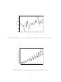
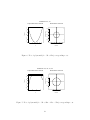
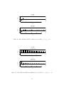
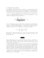
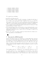
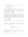
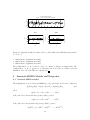
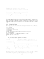
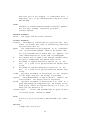
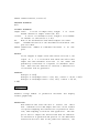
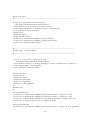
Example 1.1 Figure 1 shows seasonally adjusted quarterly time series data on savings
rate as a percent of disposable personal income for the years 1955 to 1979, as reported
by the U.S department of Commerce. An economist might analyze these data in order to
generate forecasts for future quarters. These data will be used as one of the examples in
this document.
1
15
10
5
-5
0
Billions of Dollars
1955
1957
1959
1961
1963
1965
1967
1969
Year
500
400
300
100
200
Thousands of Passengers
600
Figure 1: Savings rate as a percent of disposable personal income for the years 1955 to 1979
1949
1951
1953
1955
1957
1959
1961
Year
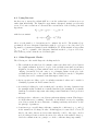
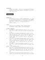
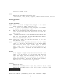
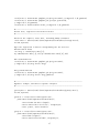
Figure 2: Number of international airline passengers from 1949 to 1960
2
Description
Process
Realization
Generates Data
Statistical Model
for the Process
Z1 , Z2 , ..., Zn
Estimates for Model
Parameters
(Stochastic Process Model)
Inferences
Forecasts
Control
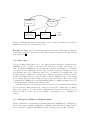
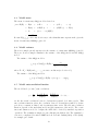
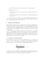
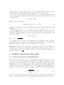
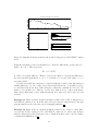
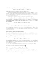
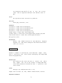
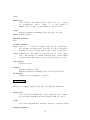
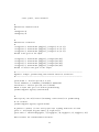
Figure 3: Schematic showing the relationship between a data-generating process and the
statistical model used to represent the process
Example 1.2 Figure 2 shows seasonal monthly time series data on the number of international airline passengers from 1949 to 1960. These data show upward trend and a strong
seasonal pattern.
1.2
Basic ideas
Box and Jenkins (1969) show how to use Auto-Regressive Integrated Moving Average
(ARIMA) models to describe model time series data, and to generate “short-term” forecasts. A univariate ARIMA model is an algebraic statement describing how observations
on a time series are statistically related to past observations and past residual error terms
from the same time series. Time-series data refer to observations on a variable that occur
in a time sequence; usually, the observations are equally spaced in time and this is required
for the Box-Jenkins methods described in this document. ARIMA models are also useful
for forecasting data series that contain seasonal (or periodic) variation. The goal is to ﬁnd
a “parsimonious” ARIMA model with the smallest number of estimated parameters needed
to ﬁt adequately the patterns in the available data.
As shown in Figure 3, a stochastic process model is used to represent the data-generating
process of interest. Data and knowledge of the process are used to identify a model. Data is
then used to ﬁt the model to the data (by estimating model parameters). After the model
has been checked, it can be used for forecasting or other purposes (e.g., explanation or
control).
1.3
Strategy for ﬁnding an adequate model
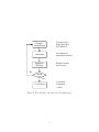
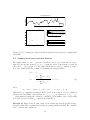
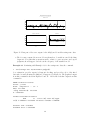
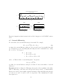
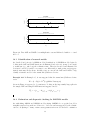
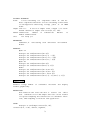
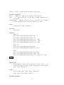
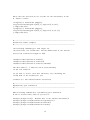
Figure 4 outlines the general strategy for ﬁnding an adequate ARIMA model. This strategy
involves three steps: tentative identiﬁcation, estimation, and diagnostic checking. Each of
these steps will be explained and illustrated in the following sections of this document.
3
Time Series Plot
Range-Mean Plot
ACF and PACF
Tentative
Identification
No
Estimation
Least Squares or
Maximum Likelihood
Diagnostic
Checking
Residual Analysis
and Forecasts
Model
ok?
Yes
Forecasting
Explanation
Control
Use the Model
Figure 4: Flow diagram of iterative model-building steps
4
1.4
Overview
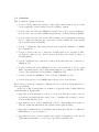
This document is organized as follows:
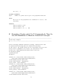
• Section 2 brieﬂy outlines the character of the S-plus software that we use as a basis
for the graphically-oriented analyses described in this document.
• Section 3 introduces the basic ARMA model and some of its properties, including a
model’s “true” autocorrelation (ACF) and partial autocorrelation functions (PACF).
• Section 4 introduces the basic ideas behind tentative model identiﬁcation, showing
how to compute and interpret the sample autocorrelation (ACF) and sample partial
autocorrelation functions (PACF).
• Section 5 explains the important practical ideas behind the estimation of ARMA
model parameters.
• Section 6 describes the use of diagnostic checking methods for detecting possible
problems in a ﬁtted model. As in regression modeling, these methods center on
residual analysis.
• Section 7 explains how forecasts and forecast prediction intervals can be generated for
ARMA models.
• Section 8 indicated how the ARMA model can be used, indirectly to model certain
kinds of nonstationary models by using transformations (e.g., taking logs) and diﬀerencing of the original time series (leading to ARIMA models).
• Section 9 extends the ARIMA models to Seasonal “SARIMA” models.
• Section 10 shows how to ﬁt SARIMA time series models to seasonal data.
Each of these sections use examples to illustrate the use of the new S-plus functions for
time series analysis.
At the end of this document there are a number of appendices that contain additional
useful information. In particular,
• Appendix A gives information on how to set up your Vincent account to use the
special time series functions (if you have been to a Statistics 451 workshop, you have
seen most this material before.
• Appendix B provides detailed instructions on how to print graphics from S-plus on
Vincent. Again, this information was explained in the Splus workshop.
• Appendix C explains the use of the Emacs Smode that allows the use of S-plus from
within Emacs—a very powerful tool.
• Appendix D provides a brief description and detailed documentation on the special
S-plus functions that have been developed especially for Statistics 451.
5
• Appendix E contains a long list of Splus commands that have been used to analyze a
large number of diﬀerent example (real and simulated) time series. These commands
also appear at the end of the Statistics 451 ﬁle splusts.examples.q. Students can
use the commands in this ﬁle to experiment with the diﬀerent functions.
2
Computer Software
The S-plus functions described in this document were designed to graphically guide the user
through the three stages (tentative identiﬁcation, estimation, and forecasting) of time-series
analysis. The software is based on S-plus. S-plus is a software system that runs under the
UNIX and MS/DOS operating systems on a variety of hardware conﬁgurations (but only
on Vincent at ISU).
2.1
S-plus concepts
S-plus is an integrated computing environment for data manipulation, calculation, and
graphical display. Among other things it has:
• An eﬀective data handling and storage facility,
• A suite of operators for calculations on arrays and, in particular, matrices.
• A large collection of intermediate tools for data analysis.
• Graphical facilities for data display either at a terminal or on hard copy.
• A well developed, simple and eﬀective programming language which includes conditionals, loops, user-deﬁned functions, and input and output facilities.
Much of the S-plus system itself is written in the S-plus language and advanced users
can add their own S-plus functions by writing in this language. This document describes
a collection of such functions for time series analysis. One does not, however, have to
understand the S-plus language in order to do high-level tasks (like using the functions
described in this document).
2.2
New S-plus functions for time series analysis
The following is a brief description of each of the S-PlusTS functions (written in the Splus
language) for time series. Some of these functions are for data analysis and model building.
Others provide properties of speciﬁed models. There are also S-PlusTS functions that use
simulation to provide experience in model building and interpretation of graphical output.
Deﬁnition of terms, instructions for use, and examples are given in the following sections.
Detailed documentation is contained in Appendix D.
• Function read.ts is used to read a time series into S-plus and construct a data
structure containing information about the time series. This data set is then used as
input to the iden and esti functions.
6
• Function iden provides graphical (and tabular) information for tentative identiﬁcation of ARMA, ARIMA, and SARIMA models. For a particular data set, speciﬁed
transformation (default is no transformation) and amount of diﬀerencing (default is
no diﬀerencing), the function provides the following:
Plot of the original data or transformed data.
If there is no diﬀerencing, range-mean plot of the transformed data, which is
used to check for nonstationary variance.
Plots of the sample ACF and PACF of the possibly transformed and diﬀerenced
time series.
• Function esti, for a speciﬁed data set and model, estimates the parameters of the
speciﬁed ARMA, ARIMA or SARIMA model and provides diagnostic checking output
and forecasts in graphical form. Graphical outputs and statistics given are:
Parameter estimates with their approximate standard errors and t-like ratios.
Estimated variance and the standard deviation of the random shocks.
Plot of the residual ACF.
Plots of the residuals versus time and residuals versus ﬁtted values.
Plot of the actual and ﬁtted values versus time and also forecasted values versus
time with their 95% prediction interval.
Normal probability plot of residuals.
• Function plot.true.acfpacf computes and plots the true ACF and PACF functions
for a speciﬁed model and model parameters.
• Function arma.roots will graphically display the roots of a speciﬁed AR or MA
deﬁning polynomial. It will plot the polynomial and the roots of the polynomial,
relative to the “unit circle.” This will allow easy assessment of stationarity (for AR
polynomials) and invertibility (for MA polynomials).
• Function model.pdq allows the user to specify, in a very simple form, an ARMA,
ARIMA, or SARIMA model to be used as input to function esti.
• Function new.model.like.tseries allows the user to specify an ARMA, ARIMA,
or SARIMA model in a form that is more general than that allowed by the simpler
function model.pdq. It allows the inclusion of high-order terms without all of the
low-order terms.
• Function add.text is useful for adding comments or other text to a plot.
• Function iden.sim is designed to give users experience in identifying ARMA models
based on simulated data from a randomly simulated model. It is also possible to
specify a particular model from which data are to be simulated.
7
• Function multiple.acf.sim allows the user to assess the variability (i.e., noise) that
one will expect to see in sample ACF functions. The function allows the user to assess
the eﬀect that realization size will have on one’s ability to correctly identify an ARMA
model.
• Function multiple.pi.sim allows the user to assess the variability (i.e., noise) that
one will expect to see in a sequence of computed prediction intervals. The function
allows the user to assess the eﬀect of sample size and conﬁdence level on the size and
probability of correctness of a simulated sequence of prediction intervals.
• Function multiple.probplot.sim allows the user to assess the variability (i.e., noise)
that one will expect to see in a sequence of probability plots. The function allows the
user to assess the eﬀect of sample size has on one’s ability to discriminate among
distributional models.
2.3
Creating a “data structure” S-plus object to serve as input to the
iden and esti functions
Before using the iden and esti functions, it is necessary to read data from an ASCII ﬁle.
The read.ts function reads data, title, time and period information, and puts all of the
information into one S-plus object, making it easy to use the data analysis functions iden
and esti. This function can be used in the “interactive” mode or in the “command” mode.
Example 2.1 To read the savings rate data introduced in Example 1.1, using the interactive mode, give the following S-plus commands and then respond to the various prompts:
> savings.rate.d <- read.ts(path="/home/wqmeeker/stat451/splus/data")
Input unix file name: savings_rate.dat
Input data title:
US Savings Rate for 1955-1980
Input response units:
Percent of Disposable Income
Input frequency: 4
Input start.year: 1955
Input start.month: 1
The ﬁle savings.rate.dat is in the /home/wqmeeker/stat451/data/ “path” (along with
a number of other stat451 data sets). You do not need to specify the path if the data is
in your /stat451 directory. When you want to input your own data, put it is an “ascii
ﬂat ﬁle” and give it a name like xxxx.dat where xxxx is a meaningful name for the time
series. Then the read.ts command will generate a data set savings.rate.d. This dataset
provides input for our other S-PlusTS functions.
Instead of answering all of the questions, another alternative is to use the “command
option” to create the input data structure.
8
Example 2.2 To read the savings rate quarterly data introduced in Example 1.1, using
the “command option” use the following command.
savings.rate.d <- read.ts(
file.name="/home/wqmeeker/stat451/data/savings_rate.dat",
title="US Savings Rate for 1955-1980",
series.units="Percent of Disposable Income", frequency=4,
start.year=1955, start.month=1,time.units="Year")
This command creates an S-plus object savings.rate.d.
Notice that, for quarterly data, the inputs frequency, start.year, and start.month
specifying the seasonality, are given in a manner that is analogous to monthly data.
Example 2.3 To read the airline passenger monthly data introduced in Example 1.2, use
the following command.
airline.d <- read.ts(file.name="/home/wqmeeker/stat451/data/airline.dat",
title="International Airline Passengers",
series.units="Thousands of Passengers", frequency=12,
start.year=1949, start.month=1,time.units="Year")
This command creates an S-plus object airline.d.
Example 2.4 To read the AT&T common stock closing prices for the 52 weeks of 1979,
use the command
att.stock.d <- read.ts(file.name="/home/wqmeeker/stat451/data/att_stock.dat",
title="1979 Weekly Closing Price of ATT Common Stock",
series.units="Dollars", frequency=1,
start.year=1, start.month=1,time.units="Week")
This command creates an S-plus object att.stock.d. Note that these data have no natural
seasonality. Thus, the inputs for frequency, start.year, start.month, are just given the
value 1.
3
ARMA Models and Properties
A time series model provides a convenient, hopefully simple, mathematical/probabilistic
description of a process of interest. In this section we will describe the class of models
known as AutoRegressive Moving Average or “ARMA” models. This class of models is particularly useful for describing and short-term forecasting of stationary time series processes.
The ARMA class of models also provides a useful starting point for developing models for
describing and short-term forecasting of some nonstationary time series processes.
9
3.1
ARMA models
The (nonseasonal) ARMA(p, q) model can be written as
φp (B)Zt = θ0 + θq (B)at
(1)
where B is the “backshift operator” giving BZt = Zt−1 , θ0 is a constant term.
φp (B) = (1 − φ1 B − φ2 B2 − · · · − φp Bp )
is the pth-order nonseasonal autoregressive (AR) operator, and
θq (B) = (1 − θ1 B − θ2 B2 − · · · − θq Bq )
is the qth-order moving average (MA) operator.
The variable at in equation (1) is the “random shock” term (also sometimes called the
“innovation” term), and is assumed to be independent over time and normally distributed
with mean 0 and variance σa2 .
The ARMA model can be written in the “unscrambled form” as
Zt = θ0 + φ1 Zt−1 + φ2 Zt−2 + · · · + φp Zt−p − θ1 at−1 − θ2 at−2 − · · · − θq at−q + at .
3.2
(2)
Stationarity and Invertibility
If p = 0, the model is a “pure MA” model and Zt is always stationary. When an ARMA
model has p > 0 AR terms, Zt is stationary if and only if all of the roots of φp (B) all lie
outside of the “unit circle.” If q = 0 the ARMA model is “pure AR” and Zt is always
invertible. When an ARMA model has q > 0 MA terms, Zt is invertible if and only if all of
the roots of θq (B) all lie outside of the “unit circle.”
The S-PlusTS function arma.roots can be used to compute and display the roots of an
AR or an MA polynomial.
Example 3.1 To ﬁnd the roots of the polynomial (1 − 1.6B − .4B2 ) use the command
> arma.roots(c(1.6,.4))
re im
dist
1 0.5495 0 0.5495
2 -4.5495 0 4.5495
>
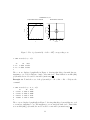
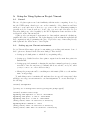
The roots are displayed graphically in Figure 5, showing that this polynomial has two real
roots, one of inside and one outside of the unit circle. Thus if this were an MA (AR)
polynomial, the model would be nonivertible (nonstationary).
Example 3.2 To ﬁnd the roots of the polynomial (1 − .5B + .1B2 ) use the command
10
Coefficients= 1.6, 0.4
Roots and the Unit Circle
•
•
-4
-20
-2
0
Imaginary Part
-10
-15
Function
-5
2
0
4
Polynomial Function versus B
-10
-8
-6
-4
-2
0
-4
B
-2
0
2
4
Real Part
Figure 5: Plot of polynomial (1 − 1.6B − .4B2 ) corresponding roots
> arma.roots(c(.5,-.1))
re
im
dist
1 2.5 1.9365 3.1623
2 2.5 -1.9365 3.1623
>
The roots are displayed graphically in Figure 6, showing that this polynomial has two
imaginary roots, both of which are outside of the unit circle. Thus if this were an MA (AR)
polynomial, the model would be invertible (stationary).
Example 3.3 To ﬁnd the roots of the polynomial (1 − .5B + .9B2 − .1B3 − .5B4 ) use the
command
> arma.roots(c(.5,-.9,.1,.5))
re
im
dist
1 0.1275 0.8875 0.8966
2 0.1275 -0.8875 0.8966
3 -1.8211 0.0000 1.8211
4 1.3662 0.0000 1.3662
>
The roots are displayed graphically in Figure 7, showing that this polynomial has two real
roots and two imaginary roots. The imaginary roots are inside the unit circle. Thus if this
were an MA (AR) polynomial, the model would be nonivertible (nonstationary).
11
Coefficients= 0.5, -0.1
Roots and the Unit Circle
0
-1
Imaginary Part
1
1.0
0.8
•
0.4
-2
0.6
Function
•
2
1.2
Polynomial Function versus B
0
1
2
3
4
5
-2
-1
B
0
1
2
Real Part
Figure 6: Plot of polynomial (1 − .5B + .1B2 ) corresponding roots
Coefficients= 0.5, -0.9, 0.1, 0.5
Roots and the Unit Circle
1
•
•
•
•
-100
-1
0
Imaginary Part
-40
-60
-80
Function
-20
0
Polynomial Function versus B
-4
-2
0
2
-1
B
0
1
Real Part
Figure 7: Plot of polynomial (1 − .5B + .9B2 − .1B3 − .5B4 ) corresponding roots
12
3.3
Model mean
The mean of a stationary AR(p) model is derived as
µZ ≡ E(Zt ) = E(θ0
+ φ1 Zt−1
+ ···
= E(θ0 ) + φ1 E(Zt−1 ) + · · ·
+ at )
+ φp E(Zt−p ) + E(at )
+ (φ1 + · · · + φp )E(Zt )
= θ0
=
+ φp Zt−p
θ0
1−φ1 −···−φp
Because E(θk at−k ) = 0 for any k, it is easy to show that this same expression also gives the
mean of a stationary ARMA(p, q) model.
3.4
Model variance
There is no simple general expression for the variance of a stationary ARMA(p, q) model.
There are, however, simple formulas for the variance of the AR(p) model and the MA(p)
model.
The variance of the AR(p) model is
γ0 ≡ σz2 ≡ Var(Zt ) ≡ E(Ż 2 ) =
σa2
φ1 ρ1 − · · · − φp ρp
where Ż = Zt − E(Zt) and ρ1 , . . . , ρp are autocorrelations (see Section 3.5).
The variance of the MA(q) model is
γ0 ≡ σz2 ≡ Var(Zt ) ≡ E(Ż 2 ) = (1 + θ12 + · · · + θq2 )σa2
3.5
Model autocorrelation function
The model-based (or “true”) autocorrelations
ρk =
E(Żt Żt+k )
γk
Cov(Zt , Zt+k )
=
,
=
γ0
Var(Zt )
Var(Zt )
k = 1, 2, . . .
are the theoretical correlations between observations separated by k time periods. This
autocorrelation function, where the correlation between observations separated by k time
periods is a constant, is deﬁned only for stationary time series. The true autocorrelation
function depends on the underlying model and the parameters of the model. The covariances and variances needed to compute the ACF can be derived by standard expectation
operations. The formulas are simple for pure AR and pure MA models. The formulas become more complicated for mixed ARMA models. Box and Jenkins (1969) or Wei (1989),
for example, give details.
13
Example 3.4 Autocovariance and Autocorrelation Functions for the MA(2) Model
The autocovariance function for an MA(2) model can be obtained from
γ1 ≡ E(Żt Żt+1 )
= E[(−θ1 at−1 − θ2 at−2 + at )(−θ1 at − θ2 at−1 + at+1 )]
= E[(θ1 θ2 a2t−1 − θ1 a2t )]
= θ1 θ2 E(a2t−1 ) − θ1 E(a2t ) = (θ1 θ2 − θ1 )σa2
Then the autocorrelation function is
ρ1 =
γ1
θ1 θ2 − θ1
=
.
γ0
1 + θ12 + θ22
Using similar operations, it is easy to show that
ρ2 =
γ2
−θ2
=
γ0
1 + θ12 + θ22
and that, in general, for MA(2), ρk = γk /γ0 = 0 for k > 2. The calculations are similar for
an MA(q) model with other values of q.
Example 3.5 Autocovariance and Autocorrelation Functions for the AR(2) Model
The autocovariance function for an AR(2) model can be obtained from
+ φ2 Żt−1
+ at+1 )]
γ1 ≡ E(Żt Żt+1 ) = E[Żt (φ1 Żt
= φ1 E(Żt2 )
+ φ2 E(Żt Żt−1 ) + E(Żt at+1 )
= φ1 γ0
+ φ2 γ1
+ 0
+ φ2 Żt
+ at+2 )]
γ2 ≡ E(Żt Żt+2 ) = E[Żt (φ1 Żt+1
= φ1 E(Żt Żt+1 ) + φ2 E(Żt2 )
+ E(Żt at+2 )
+ φ2 γ0
+ 0
= φ1 γ1
Then the autocorrelation function is ρk = γk /γ0 and ρ0 = 1, gives the AR(2) ACF
+ φ2 ρ1
ρ1 = φ1
ρ2 = φ1 ρ1
+ φ2
ρ3 = φ1 ρ2
+ φ2 ρ1
..
..
..
.
.
.
ρk = φ1 ρk−1 + φ2 ρk−2
The calculations are similar for an AR(p) model with other values of p. In general, the ﬁrst
two equations are commonly known the “Yule-Walker” equations.
3.6
Model partial autocorrelation function
The model PACF (or “true PACF”) gives the model-based correlation between observations
(Zt , Zt+k ) separated by k time periods ((k = 1, 2, 3, . . .)), accounting for the eﬀects of
14
intervening observations (Zt+1 , Zt+2 , . . . , Zt+k−1 ). The PACF function can be computed as
a function of the model (or true) ACF function. The formula for calculating the true PACF
is:
φ11 = ρ1
ρk −
k−1
φk−1 ,j ρk−j
j=1
φkk =
1−
k−1
,
k = 2, 3, . . .
(3)
φk−1 ,j ρj
j=1
where
φkj = φk−1,j − φkk φk−1,k−j ,
(k = 3, 4, . . . ;
j = 1, 2, . . . , k − 1).
This formula for computing the true PACF is based on the solution of the Yule-Walker
equations.
3.7
Computing and graphing the model (“true”) ACF and PACF functions
Plots (and tabular values) of the true ACF and PACF functions can be obtained using the
following S-plus commands
>
>
>
>
plot.true.acfpacf(model=list(ar=.95))
plot.true.acfpacf(model=list(ar=c(.78,.2)))
plot.true.acfpacf(model=list(ma=c(1,-.95)))
plot.true.acfpacf(model=list(ar=.95,ma=-.95))
The output from these commands is shown in Figures 8, 9, 10, and 11, respectively.
3.8
General behavior of ACF and PACF functions
The general behavior of the true ACF and PACF functions is easy to describe.
• For AR(p) models,
The ACF function will die down (sometimes in an oscillating manner). When
close to a stationarity boundary, the rate at which the ACF decays may be very
slow [e.g., and AR(1) model with φ = .999]. For this reason, if the ACF dies
down too slowly, it may be an indication that the process generating the data
is nonstationary.
The PACF function will “cut oﬀ” (i.e. be equal to 0) after lag p.
• For MA(q) models,
The ACF function will “cut oﬀ” (i.e. be equal to 0) after lag q.
15
True ACF
0.0
-1.0
True ACF
1.0
ar: 0.95
0
5
10
15
20
15
20
Lag
True PACF
0.0
-1.0
True PACF
1.0
ar: 0.95
0
5
10
Lag
Figure 8: True ACF and PACF for AR(1) model with φ1 = .95
True ACF
0.0
-1.0
True ACF
1.0
ar: 0.78, 0.2
0
5
10
15
20
15
20
Lag
True PACF
0.0
-1.0
True PACF
1.0
ar: 0.78, 0.2
0
5
10
Lag
Figure 9: True ACF and PACF for AR(2) model with φ1 = .78, φ2 = .2
16
True ACF
0.0
-1.0
True ACF
1.0
ma: 1, -0.95
0
5
10
15
20
15
20
Lag
True PACF
0.0
-1.0
True PACF
1.0
ma: 1, -0.95
0
5
10
Lag
Figure 10: True ACF and PACF for MA(2) model with θ1 = 1., θ2 = −.95
True ACF
0.0
-1.0
True ACF
1.0
ma: -0.95 ar: 0.95
0
5
10
15
20
15
20
Lag
True PACF
0.0
-1.0
True PACF
1.0
ma: -0.95 ar: 0.95
0
5
10
Lag
Figure 11: True ACF and PACF for ARMA(1, 1) model with φ1 = .95, θ1 = −.95
17
The PACF function will die down (sometimes in an oscillating manner).
• For ARMA(p, q) models,
The ACF function will die down (sometimes in an oscillating manner) after lag
max(0, q − p).
The PACF function will die down (sometimes in an oscillating manner)after lag
max(0, p − q).
As described in Section 4, estimates of the the ACF and PACF, computed from data,
can be compared with the expected patterns of the “true” ACF and PACF functions and
used to help suggest appropriate models for the data.
4
Tentative Identiﬁcation
At the tentative identiﬁcation stage we use sample autocorrelation function (ACF) and the
sample partial autocorrelation function (PACF). The sample ACF and sample PACF can
be thought of as estimates of similar theoretical (or “true”) ACF and PACF functions that
are characteristic of some underlying ARMA model. (Recall from Sections 3.5 and 3.6 that
the “true” ACF and “true” PACF can be computed as a function of a speciﬁed model and
its parameters.)
At the beginning of the identiﬁcation stage, the model is unknown so we tentatively
select one or more ARMA models by looking at graphs of the sample ACF and PACF
computed from the available data. Then we choose a tentative model whose associated true
ACF and PACF look like the sample ACF and PACF calculated from the data. To choose a
ﬁnal model we proceed to the estimation and checking stages, returning to the identiﬁcation
stage if the tentative model proves to be inadequate.
4.1
Sample autocorrelation function
The sample ACF is computed from a time-series realization Z1 , Z2 , . . . , Zn and gives the
observed correlation between pairs of observations (Zt , Zt+k ) separated by various time
spans (k = 1, 2, 3, . . .). Each estimated autocorrelation coeﬃcient ρk is an estimate of the
corresponding parameter ρk . The formula for calculating the sample ACF is:
n−k
ρk =
t=1
(Zt − Z̄)(Zt+k − Z̄)
n
(Zt − Z̄)2
,
k = 1, 2, . . . .
t=1
One can begin to make a judgment about what ARIMA model(s) might ﬁt the data by
examining the patterns in the estimated ACF. The iden command automatically plots the
speciﬁed time series and provides plots of the sample ACF and PACF.
18
US Savings Rate for 1955-1980
4
5
6
w
7
8
9
w= Percent of Disposable Income
1960
1970
1980
time
ACF
0.0
-1.0
2.5
ACF
3.0
0.5
1.0
Range-Mean Plot
10
20
30
Lag
2.0
Range
0
0.5
0.5
0.0
-1.0
1.0
Partial ACF
1.0
1.5
PACF
4.5
5.0
5.5
6.0
6.5
7.0
7.5
0
10
Mean
20
30
Lag
Figure 12: Plot of savings rate data along with a range-mean plot and plots of sample ACF
and PACF
4.2
Sample partial autocorrelation function
The sample PACF φ̂11 , φ̂22 , · · · gives the correlation between ordered pairs (Zt , Zt+k ) separated by various time spans (k = 1, 2, 3, . . .) with the eﬀects of intervening observations
(Zt+1 , Zt+2 , . . . , Zt+k−1 ) removed. The sample PACF function can be computed as a function of the sample ACF. The formula for calculating the sample PACF is:
φ̂11 = ρ1
ρk −
k−1
φ̂k−1 ,j ρk−j
j=1
φ̂kk =
1−
k−1
,
k = 2, 3, . . .
(4)
φ̂k−1 ,j ρj
j=1
where
φ̂kj = φ̂k−1,j − φ̂kk φ̂k−1,k−j
(k = 3, 4, . . . ;
j = 1, 2, . . . , k − 1)
This method of computing the sample PACF is based on the solution of a set of equations
known as the Yule-Walker equations that give ρ1 , ρ2 , . . . , ρk as a function of φ1 , φ2 , . . . , φk .
Each estimated partial autocorrelation coeﬃcient φ̂kk is an estimate of the corresponding
model-based (“true”) PACF φkk computed as shown in (3).
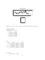
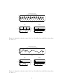
Example 4.1 Figure 12 shows iden output for the savings rate data along with a rangemean plot (that will be explained later) and plots of sample ACF and PACF. The command
used to generate this output was
19
Wolfer Sunspots
0
50
w
100
150
w= Number of Spots
1780
1800
1820
1840
1860
time
ACF
0.0
-1.0
120
ACF
140
0.5
1.0
Range-Mean Plot
10
100
Range
0
20
30
Lag
40
0.5
0.0
-1.0
60
Partial ACF
1.0
80
PACF
20
30
40
50
60
70
0
Mean
10
20
30
Lag
Figure 13: Plot of sunspot data along with a range-mean plot and plots of sample ACF and
PACF
>
iden(savings.rate.d)
The sample ACF and PACF plots show that the ACF dies down and that the PACF cuts
oﬀ after one lag. This matches the pattern of an AR(1) model and suggests this model as
a good starting point for modeling the savings rate data.
4.3
Understanding the sample autocorrelation function
As explained in Section 4.1, the sample ACF function plot show the correlation between
observations separated by k = 1, 2, . . . time periods. For another example, Figure 13 gives
the iden output from the Wolfer sunspot time series. In order to better understand an
ACF, or to investigate the reasons for particular spikes in a sample ACF, it is useful to
obtain a visualization of the individual correlations in an ACF. Figure 14 was obtained by
using the command
>
show.acf(spot.d)
5
Estimation
Computer programs are generally needed to obtain estimates of the parameters of the
ARMA model chosen at the identiﬁcation stage. Estimation output can be used to compute
quantities that can provide warning signals about the adequacy of our model. Also at this
stage the results may also indicate how a model could be improved and this leads back to
the identiﬁcation stage.
20
50
50
•
0
•
150
0
150
50
100
100
Series lag 4
•
50
•• • • •
•
•
•• • •
•
•
•••• •• • •• •
••
•
•
••
•••• •
•
••• ••••••• • • •
•
• •
•••
• •
•• • •
••
•
•
•
•
•
•
• • •• •• ••• • •
• ••
•
• ••
•
0
150
• •
•
100
100
50
Series lag 3
0
•
50
150
100
0
150
•
•
150
•
•
••
•
•• •
••
•••• ••
•
••• •
•
•• • ••••
• •
• •
• •
••••••• • • • •• • • • •
• •
• •
•••
•• •
•• •
• •• • •
••
•
•
•• • •• ••• •
• •
••• •
•• • •
0
50
100
0
100
140
20
60
series
100
•
50
• •
140
•
•
•
•
•
•
•
••
•
• •
• • • •••• ••• •
•
•
••
•• •
•
• • ••
•
• •• • •• •
• •
• •• • •
•
••••• ••• •• •
•
•• •
•••••••• •
0
20
60
series
100
••
• •
140
150
100
Series lag 9
50
0
•
•
• •
•
• • •••• •
•
•
•
• •• •
•
•• ••• • •• •
• • •• ••• • •• •
••• •••
•
•• ••• •• ••••• • •
•
••• • •••• ••
0
20
60
100
•
••
•
•
140
series
Lag 13
Series : timeseries
•
•
0
•
1.0
100
Series lag 8
50
•
150
•
•
•
series
•
•
• • •
•
•
••
•• • •
••
• • ••••
•
•••
•
• • •
• • • •• • • • • •• ••
• • • •
•• • •
• •••• •
• •
••
•••••••• ••• ••
• •
•
•
100
•
•
• •
• •
ACF
0.2
0.6
100
•
50
•
150
•
••
Series lag 12
•
• •
•
•
•
•
• • •• •
••
• ••• • •
•
• • ••••
•• •••
• •• • ••
•
••
•
•
•• ••• •
• •• •
•••••• •••• •••• • •
•
•
•
0
0
100
150
•
0
•
•
150
•
•
••
•
• •
• • • ••• •
•
•••
•
• ••• • • • • • • •
••
•
• •
• • •• •• •••
• •
••••• •• •• •• • •••
• • ••• •••• ••
•
Lag 12
•
•••
•
100
•
50
••
•
•• • •
• ••
••• •••• ••
• •• • ••
• •
• •
•• • •
•• •••• • • •• • • •
••••• • •••• •
•
•
Series lag 11
• •
••
•
•• • •
• •
•
•
100
•
•
•• •
•
•
150
20
60
100
•
•
•
• ••
140
-0.2
50
0
100
Series lag 7
50
0
•
•
••
series
150
150
••
series
150
•
•
• •
• • • ••
•• • •
• ••
• ••
•
•
••••• • • •
•
••
•• •
• •
•
• •• • • •• •
•••• • • •• • •• ••
••• ••••• •• ••
Lag 11
••
•
60
100
•
series
•
•
••
•• •
•
50
50
•
•
Series lag 13
0
0
100
Series lag 6
150
•
•
•
•
•• •
•••• • •
0
100
•
•
•
•
• •
•••
•
• •••• • •
• •
• •
•
• •
•
•
•• • • • • •• •
•
•••••
• • ••
••
•• •
• •
••• •
••
•
••• ••• ••
•
•
•
•
•• • •••• ••••• • •• •
• ••
150
series
Lag 9
150
series
Lag 8
150
series
Lag 7
•
100
50
Series lag 10
0
100
•
•
•
•
•
•
Lag 4
•
•
series
•
20
•
•••
•
•••• •
••• •
•••• • •• • •
••
•
•
• •• •
••• • • • • •
••• ••• •• •
•••• • • • • •
••
•••
•• ••••• • •••• •• • •
•
•
•
••
Lag 6
Lag 10
0
•
•
Lag 3
•
Lag 5
series
•
•
•
•
•
•
timeseries
50
•
•
• •
Series lag 2
• •
•
•
• •• •
•••
••
••• •• • ••••
•
•
•
•
•
•
•• ••• •••• • •
••• • • • • •
• •
•• •
•
••• • ••••
••••
••••••••••• • •
•••
0
•
••
•
Lag 2
•
•
50
150
100
150
•
• •
•
•••
•• • •
••
• ••• •
•
•
•
•••• ••
•
• • •
•• • •
•
• • ••
••••••••
•
• •
•
• •
•• • •
• •• •••
•
•• •
•
•
• •
•
••
••
• •• •••••• • • • • • •
0
50
Series lag 1
100
50
100
50
0
Series lag 5
150
0
0
•••
•••••
•••
•••
••••
••••
••
••••
•
•
•
••
•••
••
••••••
••••
0
100
50
0
timeseries
150
Lag 1
•
•
••
•••
0
5
10
Lag
15
20
series
Figure 14: Plot of the show.acf command showing graphically the correlation between
sunspot observations separated by k = 1, 2, . . . 12 years
The basic idea behind maximum likelihood (ML) estimation is to ﬁnd, for a given set
of data, and speciﬁed model, the combination of model parameters that will maximize the
“probability of the data.” Combinations of parameters giving high probability are more
plausible than those with low probability. The ML estimation criteria is the preferred
method. Assuming a correct model the likelihood function from which ML estimates are
derived reﬂects all useful information about the parameters contained in the data.
Estimated coeﬃcients are nearly always correlated with one another. Estimates of the
“parameter correlations” provide a useful diagnostic. If estimates are highly correlated,
the estimates are heavily dependent on each other and tend to be unstable (e.g., slight
changes in data can cause large changes in estimates). If one or more of the correlations
among parameters is close to 1, it may be an indication that the model contains too many
parameters.
6
Diagnostic Checking
At the diagnostic-checking stage we check to see if the tentative model is adequate for its
purpose. A tentative model that fails one or more diagnostic tests is rejected. If the model
is rejected we repeat the cycle of identiﬁcation, estimation and diagnostic checking in an
attempt to ﬁnd a better model. The most useful diagnostic checks consist of plots of the
residuals, plots of functions of the residuals and other simple statistics that describe the
adequacy of the model.
21
6.1
Residual autocorrelation
In an ARMA model, the random shocks at are assumed to be statistically independent so
at the diagnostic-checking stage we use the observed residuals at to test hypotheses about
the independence of the random shocks. In time series analysis, the observed residuals are
deﬁned as the diﬀerence between Zt and the one-step-ahead forecast for Zt (see Section 7).
In order to check the assumption that the random shocks (at ) are independent, we
a2 , . . . . The
compute a residual ACF from the time series of the observed residuals a1 , formula for calculating the ACF of the residuals is:
n−k
ρk (
a) =
t=1
(ât − ā)(
at+k − ā)
n
(
at − ā)2
,
k = 1, 2, . . ..
t=1
a) that are importantly diﬀerent
where ā is the sample mean of the at values. Values of ρk (
from 0 (i.e., statistically signiﬁcant) indicate a possible deviation from the independence
assumption. To judge statistical signiﬁcance we use Bartlett’s approximate formula to
estimate the standard errors of the residual autocorrelations. The formula is:


Sρk (a)
1/2
k−1

= [1 + 2
ρj (
a)2 ]/n
.


j=1
Having found the estimated standard errors of ρk (â), we can test, approximately, the null
hypothesis H0 : ρk (a)=0 for each residual autocorrelation coeﬃcient. To do this, we use a
standard t-like ratio
t=
a) − 0
ρk (
.
Sρk (a)
In large samples, if the true ρk (a) = 0, then this t-like ratio will follow, approximately, a
standard normal distribution. Thus with a large realization, if H0 is true, there is only
about a 5% chance of having t outside the range ±2, and values outside of this range will
indicate non-zero autocorrelation.
The estimated standard errors are sometimes seriously overstated when applying Bartlett’s
formula to residual autocorrelations. This is especially possible at the very short lags (lags
1,2 and perhaps lag 3). Therefore we must be very careful in using the t-like ratio especially those at the short lags. Pankratz (1983) suggests using “warning” limits of ±1.50 to
indicate the possibility of a signiﬁcant spike in the residual ACF. Interpretation of sample
ACF’s is complicated because we are generally interpreting, simultaneously, a large number
a) values. As with the interpretation of ACF and PACF functions of data during the
of ρk (
identiﬁcation stage, the t-like ratios should be used only as guidelines for making decisions
during the process of model building.
22
6.2
Ljung-Box test
Another way to assess the residual ACF is to test the residual autocorrelations as a set
rather than individually. The Ljung-Box approximate chi-squared statistic provides such
a test. For k autocorrelations we can assess the reasonableness of the following joint null
hypothesis;
H0 : ρ1 (a) = ρ2 (a) = . . . = ρK (a) = 0
with the test statistic
K
a)
Q = n(n + 2) (n − k)−1 ρ2k (
k=1
where n is the number of observations used to estimate the model. The statistic Q approximately follows a chi-squared distribution with (k − p) degrees of freedom, where p is
the number of parameters estimated in the ARIMA model. If this statistic is larger than
χ2(1−α;k−p) , the 1 − α quantile of the chi-square distribution with k − p degrees of freedom,
there is strong evidence that the model is inadequate.
6.3
Other Diagnostic Checks
The following are other useful diagnostic checking methods.
• The residuals from a ﬁtted model constitute a time-series that can be plotted just as
the original realization is plotted. A plot of the residuals versus time is sometimes
helpful in detecting problems with the ﬁtted model and gives a clear indication of
outlying observations. It is also easier to see a changing variance in the plot of the
residuals then in a plot of the original data. The residual plot can also be helpful in
detecting data errors or unusual events that impact a time series.
• As in regression modeling, a plot of residuals versus ﬁtted values can be useful for
identifying departures from the assumed model.
• A normal probability plot of the residuals can be useful for detecting departures from
the assumption that residuals are normally distributed (the assumption of normally
distributed residuals is important when using normal distribution based prediction
intervals.
• Adding another coeﬃcient to a model may result in useful improvement. This diagnostic check is known as “overﬁtting.” Generally, one should have a reason for expanding
a model in a certain direction. Otherwise, overﬁtting is arbitrary and tends to violate
the principle of parsimony.
• Sometimes a process will change with time, causing the coeﬃcients (e.g., φ1 and θ1 )
in the assumed model change in value. If this happens, forecasts based on a model
ﬁtted to the entire data set are less accurate than they could be. One way to check a
model for this problem is to ﬁt the chosen model to subsets of the available data (e.g.,
divide the realization into two parts) to see if the coeﬃcients change importantly.
23
US Savings Rate for 1955-1980
Model: Component 1 :: ar: 1 on w= Percent of Disposable Income
1
-1
0
Residuals
2
3
Residuals vs. Time
1960
1970
1980
Time
Residual ACF
1.0
Residuals vs. Fitted Values
•
• • •
• • •• •
• • • •
• • •
• •
•
•
•
•
•
•
••
•
• •
•
•
••
•
•
•
•
•
•
•
• •
• •
• •
•• • •
••
•
•
•
• •
•
•
5
••
•
•
6
0.0
•
•
•
•
•
• •
• • •
•
•
• •
•
•
• • • • •
•
ACF
•
•
-0.5
• •
7
8
9
-1.0
1
-1
•
•
• •
•
0
Residuals
2
0.5
3
•
0
Fitted Values
10
20
30
Lag
Figure 15: First part of the esti output for the AR(1) model and the savings rate data.
• The forecasts computed from a model can, themselves, be useful as a model-checking
diagnostic. Forecasts that seem unreasonable, relative to past experience and expert
judgment, should suggest doubt about the adequacy of the assumed model.
Example 6.1 Continuing with Example 4.1, for the savings rate data, the command
>
esti(savings.rate.d,model=model.pdq(p=1))
does estimation, provides output for diagnostic checking, and provides a plot of the ﬁtted
data and forecasts, all using the AR(1) model suggested by Figure 12. The graphical output
from this command is shown in Figures 15 and 16. Abbreviated tabular output from this
command is
ARIMA estimation results:
Series: y.trans
Model: Component 1 :: ar: 1
AICc: 217.3166
-2(Log Likelihood): 215.3166
S: 0.6881749
Parameter Estimation Results
MLE
se t.ratio 95% lower 95% upper
ar(1) 0.8146081 0.05715026 14.25379 0.7025935 0.9266226
Constant term: 6.167464
Standard error: 0.06780789
24
US Savings Rate for 1955-1980
Model: Component 1 :: ar: 1 on w= Percent of Disposable Income
Actual Values * * * Fitted Values * * * Future Values
* * 95 % Prediction Interval * *
•
8
•
•
•
•
•
• •
•
6
•
•
•
•
•
•
•
•
•
• ••
••
•
•
•
•
•
•
•
•
•
• •
•
•
•
•
•
•
•
•
•
•
•
•
•
•
•
•
•
• • •
••
•
•
•
•
• •
•
•
•
•
•
•
•
•
•
•
•
•
•
• •
•
• •
• •
•
•
•
•
•
•
•
•
•
•
•
•
•
•
•
••
•
•
•
•
• •• • • •• • • •
•• • •
• •
••
•
•
•
•
4
Percent of Disposable Income
•
•
•
1955
1960
1965
1970
1975
1980
1985
Index
Normal Probability Plot
•
0
-1
Normal Scores
1
2
•
-2
•
•
•
•
• ••
••
••
••
••
••
•••
•
•
•
•
•••
•••
•••
••••
•••
••
••
•••
• ••
•
•
••
••
••
••
•
•
•
••
••
••
•
-1
0
1
2
3
Residuals
Figure 16: Second part of the esti output for the AR(1) model and the savings rate data.
t-ratio: 90.95497
Ljung-Box Statistics
dof Ljung-Box
p-value
5 10.11577 0.07202058
6 10.83296 0.09367829
7 11.26102 0.12763162
8 11.35323 0.18247632
9 12.48835 0.18715667
.
.
.
ACF
Lag
ACF
se
t-ratio
1
1 -0.15321802 0.09853293 -1.55499303
2
2 0.26128739 0.10081953 2.59163466
3
3 -0.03345993 0.10719249 -0.31214809
4
4 -0.03554756 0.10729385 -0.33131035
5
5 0.01055575 0.10740813 0.09827701
.
.
.
Forecasts
Lower Forecast
Upper
25
1
2
3
4
5
.
.
.
2.645728
2.657691
2.769109
2.904987
3.039914
3.994526
4.397372
4.725533
4.992855
5.210618
5.343324
6.137053
6.681956
7.080724
7.381323
The output shows several things.
• Overall, the model ﬁts pretty well.
• There is an outlying observation. It would be interesting to determine the actual cause of
the observation. One can expect that unless something special is done to accommodate
this observation, that it will remain an outlier for all ﬁtted models. It useful (perhaps even
important) to, at some point, to repeat the analysis with the ﬁnal model, adjusting this
outlier to see if such an adjustment has an important eﬀect on the ﬁnal conclusion(s).
• As seen in Figure 16, the forecasts always lag the actual values about 1 time period. This
suggests that the model might be improved.
• The residual ACF function has some large spikes a low lags, indicating that there is some
evidence that the AR(1) model does not adequately explain the correlational structure.
This suggests adding another term or terms to the model. One might, for example, try an
ARMA(1,1) model next.
• Except for the outlier, the normal probability plot indicates that the residuals seem to
follow, approximately, a normal distribution.
7
Forecasts for ARMA models
An important application in time-series analysis is to forecast the future values of the given
time series. A forecast is characterized by its origin and lead time. The origin is the time
from which the forecast is made (usually the last observation in a realization) and the lead
time is the number of steps ahead that the series is forecast. Thus, the forecast of the
future observation Zt+l made from origin t going ahead l time periods, is denoted by Zt (l).
Starting with the unscrambled ARMA model in (2), an intuitively reasonable forecast can
be computed as
Zt (l) = θ0 + φ1 [Zt−1+l ] + φ2 [Zt−2+l ] + · · · + φp [Zt−p+l ]
− θ1 [at−1+l ] − θ2 [at−2+l ] − · · · − θq [at−q+l ]
(5)
(6)
For the quantities inside the [ ], substitute the observed values if the value has been observed
(i.e., if the subscript of Z or a on the right-hand side is less than the forecast origin t)
substitute in the observed value. If the quantity has not been observed (because it is in
the future), then substitute in the forecast for this value (0 for a future a and a previously
26
computed Zt (l) for a future value of Z). Box and Jenkins (1969) show that forecast is
optimal in the sense that it minimizes the mean squared error of the forecasts.
A forecast error for predicting Zt with lead time l (i.e., forecasting ahead l time periods)
is denoted by et (l) and deﬁned as the diﬀerence between an observed Zt and its forecast
counterpart Zt (l):
t (l).
et (l) = Zt − Z
This forecast error has variance
2
Var[et (l)] = σa2 (1 + ψ12 + . . . + ψl−1
)
(7)
where the ψi coeﬃcients are the coeﬃcients in the random shock (inﬁnite MA) form of the
ARIMA model.
If the random shocks (i.e., the at values) are normally distributed and if we have an
appropriate ARIMA model, then our forecasts and the associated forecast errors are approximately normally distributed. Then an approximate 95% prediction interval around
any forecast will be
Zt (l) ± 1.96Set (l)
where Set (l) = Var[et (l)].
t (l) and Se (l) depend on the unknown model parameters. With reasonably
Both Z
t
large samples, however, adequate approximate prediction intervals can be computed by
substituting estimates computed from model-ﬁtting into (5) and (7).
Example 7.1 Figure 16 shows forecasts for the savings rate data. The forecasts start low,
but increase to an asymptote, equal to the estimated mean of the time series. The set of
prediction intervals gets wider, with the width also reaching a limit (approximately 1.96
times the estimate of σZ ).
8
8.1
Modeling Nonstationary Time Series
Variance stationarity and transformations
Some time series data exhibit a degree of variability that changes through time (e.g., Figure 2. In some cases, especially when variability increases with level, such series can be
transformed to stabilize the variance before being modeled with the Univariate Box-JenkinsARIMA method. A common transformation involves taking the natural logarithms of the
original series. This is appropriate if the variance of the original series is approximately proportional to the mean. More generally, one can use the family of Box-Cox transformations,
i.e.,
(Z ∗ +m)γ −1
t
γ = 0
γ
(8)
Zt =
∗
log(Zt + m) γ = 0
where Zt∗ is the original, untransformed time series and γ is primary transformation parameter. Sometimes the Box-Cox power transformation is presented as Zt = (Zt∗ + m)γ .
27
The more complicated form in (8) has the advantage of being monotone increasing in Zt∗
for any γ and
(Z ∗ + m)γ − 1
lim t
= log(Zt∗ + m).
γ→0
γ
The quantity m is typically chosen to be 0 but can be used to shift a time series (usually
upward) before transforming. This is especially useful when there are some values of Zt∗ that
are negative, 0, or even close to 0. This is because the log of a nonpositive number or a noninteger power of a negative number is not deﬁned. Moreover, transformation of numbers
close to 0 can cause undesired shifts in the data pattern. Shifting the entire series upward
by adding a constant m can have the eﬀect of equalizing the eﬀect of a transformation
across levels.
8.2
Using a range-mean plot to help choose a transformation
We use a range-mean plot to help detect nonstationary variance. A range-mean plot is
constructed by dividing the time series into logical subgroups (e.g. years for 12 monthly
observations per year) and computing the mean and range in each group. The ranges
are plotted against the means to see if the ranges tend to increase with the means. If
the variability in a time series increases with level (as in percent change), the range-mean
plot will show a strong positive relationship between the sample means and the sample
variances for each period in the time series. If the relationship is strong enough, it may be
an indication of the need for some kind of transformation.
Example 8.1 Returning to savings rate data (see Example 4.1), the range-mean plot in
Figure 12 shows that, other than the outlying value, there is no strong relationship between
the mean and ranges. Thus there is no evidence of need for a transformation for these data.
Example 8.2 Figure 17 shows iden output of monthly time series data giving the number
of international airline passengers between 1949 and 1960. The command used to make this
ﬁgure is
> iden(airline.d)
The range and mean of the 12 observations within each year were computed and plotted.
This plot shows clearly the strong relationship between the ranges and the means. Figure 18
shows iden output for the logarithm of the number of passengers. The command used to
make this ﬁgure is
> iden(airline.d,gamma=0)
This ﬁgure shows that the transformation has broken the strong correlation and made the
amount of variability more stable over the realization.
When interpreting the range-mean plot and deciding on an appropriate transformation,
we have to remember that doing a transformation aﬀects many parts of a time series model,
for example,
28
International Airline Passengers
100
200
300
w
400
500
600
w= Thousands of Passengers
1949
1950
1951
1952
1953
1954
1955
1956
1957
1958
1959
1960
1961
time
ACF
0.0
-1.0
200
ACF
0.5
1.0
Range-Mean Plot
10
20
150
Range
0
30
Lag
0.5
0.0
-1.0
50
Partial ACF
100
1.0
PACF
200
300
400
0
10
20
Mean
30
Lag
Figure 17: Plot of the airline data along with a range-mean plot and plots of sample ACF
and PACF
International Airline Passengers
w
5.0
5.5
6.0
6.5
w= log(Thousands of Passengers)
1949
1950
1951
1952
1953
1954
1955
1956
1957
1958
1959
1960
1961
time
ACF
0.0
-1.0
0.45
ACF
0.5
1.0
Range-Mean Plot
10
20
30
Lag
0.40
PACF
0.5
0.0
-1.0
0.35
Partial ACF
1.0
Range
0
4.8
5.0
5.2
5.4
5.6
5.8
6.0
6.2
Mean
0
10
20
30
Lag
Figure 18: Plot of the logarithms of the airline data along with a range-mean plot and plots
of sample ACF and PACF
29
• The relationship between level (e.g., mean) and spread (e.g., standard deviation) of
data about the ﬁtted model,
• The shape of any trend curve, and
• The shape of the distribution of residuals.
We must be careful that a transformation to ﬁx one problem will not lead to other
problems. The range-mean plot only looks at the relationship between variability and level.
For many time series it is not necessary or even desirable to transform so that the correlation
between ranges and means is zero. Generally it is good practice to compare ﬁnal results of
an analysis by trying diﬀerent transformations.
8.3
Mean stationarity and diﬀerencing
ARMA models are most useful for predicting stationary time-series. These models can, however, be generalized to ARIMA models that have “integrated” random walk type behavior.
Thus ARMA models can be generalized to ARIMA models that are useful for describing
certain kinds (but not all kinds) of nonstationary behavior. In particular, an integrated
ARIMA model can be changed to a stationary ARMA model using a diﬀerencing operation. Then we ﬁt an ARMA model to the diﬀerenced data. Diﬀerencing involves calculating
successive changes in the values of a data series.
8.4
Regular diﬀerencing
To diﬀerence a data series, we deﬁne a new variable (Wt ) which is the change in Zt from
one time period to the next; i.e.,
Wt = (1 − B)Zt = Zt − Zt−1
t = 2, 3, . . . , n.
(9)
This “working series” Wt is called the ﬁrst diﬀerence of Zt . We can also look at diﬀerencing
from the other side. In particular, rewriting (9) and using successive resubstitution (i.e.,
using Wt−1 = Zt−1 − Zt−2 ) gives
Zt = Zt−1 + Wt
= Zt−2 + Wt−1 + Wt
= Zt−3 + Wt−2 + Wt−1 + Wt
= Zt−4 + Wt−3 + Wt−2 + Wt−1 + Wt
and so on. This shows why we would say that a model with a (1 − B) diﬀerencing term is
“integrated.”
If the ﬁrst diﬀerences do not have a constant mean, we might try a new Wt , which will
be the second diﬀerences of Zt , i.e.,
Wt = (Zt − Zt−1 ) − (Zt−1 − Zt−2 ) = Zt − 2Zt−1 + Zt−2 ,
30
t = 3, 4, . . . , n.
1979 Weekly Closing Price of ATT Common Stock
w
52
54
56
58
60
62
64
w= Dollars
0
10
20
30
40
50
time
ACF
0.0
-1.0
4.0
ACF
4.5
0.5
1.0
Range-Mean Plot
10
20
30
Lag
3.5
Range
0
0.5
0.0
-1.0
2.5
Partial ACF
1.0
3.0
PACF
54
56
58
60
62
0
Mean
10
20
30
Lag
Figure 19: Output from function iden for the weekly closing prices for 1979 AT&T common
stock
Using the back shift operator as shorthand, (1 − B) is the diﬀerencing operator since (1 −
B)Zt = Zt − Zt−1 . Then, in general,
Wt = (1 − B)d Zt
is a dth order regular diﬀerence. That is, d denotes the number of nonseasonal diﬀerences.
For most practical applications, d = 0 or 1. Sometimes d = 2 is used but values of d > 2
are rarely useful.
For time series that have integrated or random-walk-type behavior, ﬁrst diﬀerencing is
usually suﬃcient to produce a time series with a stationary mean; occasionally, however,
second diﬀerencing is also used. Diﬀerencing more than twice virtually never needed. We
must be very careful not to diﬀerence a series more than needed to achieve stationarity.
Unnecessary diﬀerencing creates artiﬁcial patterns in a data series and reduces forecast
accuracy.
Example 8.3 Figure 19 shows output from function iden for the weekly closing prices for
1979 AT&T common stock. Both the time series plot and the range-mean plot strongly
suggests that the mean of the time series is changing with time.
Example 8.4 Figure 20 shows output from function iden for the changes (or ﬁrst diﬀerences) in the weekly closing prices for 1979 AT&T common stock. These plots indicate
that the changes in weekly closing price have a distribution that could be modeled with a
constant-mean ARMA model.
31
-2
0
w
1
2
3
1979 Weekly Closing Price of ATT Common Stock
w= (1-B)^ 1 Dollars
0
10
20
30
40
50
time
-1.0
0.0
Partial ACF
0.0
-1.0
ACF
1.0
PACF
1.0
ACF
0
10
20
30
0
10
Lag
20
30
Lag
Figure 20: Output from function iden for the weekly closing prices for 1979 AT&T common
stock
8.5
Seasonal diﬀerencing
For seasonal models, seasonal diﬀerencing is often useful. For example,
Wt = (1 − B12 )Zt = Zt − Zt−12
(10)
is a ﬁrst-order seasonal diﬀerence with period 12, as would be used for monthly data with
12 observations per year. Rewriting (10) and using successive resubstitution (i.e., using
Wt−12 = Zt−12 − Zt−24 ) gives
Zt = Zt−12 + Wt
= Zt−24 + Wt−12 + Wt
= Zt−36 + Wt−24 + Wt−12 + Wt
and so on. This is a kind of “seasonal integration.” In general,
Wt = (1 − BS )D Zt
is a Dth order seasonal diﬀerence with period S where D denotes the number of seasonal
diﬀerences.
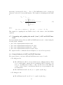
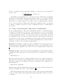
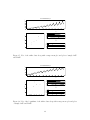
Example 8.5 Refer to Figure 18. This ﬁgure shows plots of the logarithms of the airline
with no diﬀerencing of the time series and provides strong evidence of nonstationarity.
Figure 22, 21, and 23, shows similar outputs from function iden with diﬀerencing schemes
d = 1, D = 0, d = 0, D = 1, and d = 1, D = 1, respectively. The commands used to make
these ﬁgures were
32
0.0
-0.2
w
0.2
International Airline Passengers
w= (1-B)^ 1 log( Thousands of Passengers )
1949
1950
1951
1952
1953
1954
1955
1956
1957
1958
1959
1960
1961
time
-1.0
0.0
Partial ACF
0.0
-1.0
ACF
1.0
PACF
1.0
ACF
0
10
20
30
0
10
Lag
20
30
Lag
Figure 21: Output from function iden for the log of the airline data with diﬀerencing scheme
d = 1, D = 0
0.0
w
0.2
International Airline Passengers
w= (1-B^ 12 )^ 1 log( Thousands of Passengers )
1950
1951
1952
1953
1954
1955
1956
1957
1958
1959
1960
1961
time
-1.0
0.0
Partial ACF
0.0
-1.0
ACF
1.0
PACF
1.0
ACF
0
10
20
30
0
Lag
10
20
30
Lag
Figure 22: Output from function iden for the log of the airline data with diﬀerencing scheme
d = 0, D = 1
33
0.0
-0.15
w
0.10
International Airline Passengers
w= (1-B)^ 1 (1-B^ 12 )^ 1 log( Thousands of Passengers )
1950
1951
1952
1953
1954
1955
1956
1957
1958
1959
1960
1961
time
-1.0
0.0
Partial ACF
0.0
-1.0
ACF
1.0
PACF
1.0
ACF
0
10
20
30
0
10
Lag
20
30
Lag
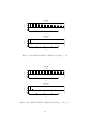
Figure 23: Output from function iden for the log of the airline data with diﬀerencing scheme
d = 1, D = 1
> iden(airline.d,gamma=0,d=1,D=0)
> iden(airline.d,gamma=0,d=0,D=1)
> iden(airline.d,gamma=0,d=1,D=1)
The results with d = 1, D = 0 and d = 0, D = 1 continue to indicate nonstationarity. The
results with d = 1, D = 1 appears to be stationary. In Section 10.2 we will ﬁt a seasonal
ARMA model to the data diﬀerenced in this way.
9
Seasonal ARIMA Models and Properties
9.1
Seasonal ARIMA model
The multiplicative period S seasonal ARIMA (p, d, q) × (P, D, Q)S model can be written as
Φp (BS )φp (B)(1 − B)d (1 − BS )D Zt = Θq (BS )θq (B)at
where
φp (B) = (1 − φ1 B − φ2 B 2 − · · · − φp Bp )
is the pth-order nonseasonal autoregressive (AR) operator;
θq (B) = (1 − θ1 B − θ2 B2 − · · · − θq Bq )
is the qth-order nonseasonal moving average (MA) operator;
ΦP (BS ) = (1 − ΦS BS − Φ2S B2S − · · · − ΦP S BP S )
34
(11)
is the Qth-order period S seasonal autoregressive (AR) operator;
ΘQ (BS ) = (1 − ΘS BS − Θ2S B2S − . . . − ΘQS BQS )
is the P th-order period S seasonal moving average (MA) operator.
The variable at in equation (11) is again the random shock element, assumed to be independent over time and normally distributed with mean 0 and variance σa2 . The lower-case
letters (p,d,q) indicate the nonseasonal orders and the upper-case letters (P,D,Q) indicate
the seasonal orders of the model.
The general seasonal model can also be written an “unscrambled form” as
Zt = φ∗1 Zt−1 + φ∗2 Zt−2 + · · · + φ∗p∗ Zt−p∗ − θ1∗ at−1 − θ2∗ at−2 − · · · − θq∗∗ at−q∗ + at
where the values of coeﬃcients like φ∗p∗ and θq∗∗ need to be computed from the expansion
(including diﬀerencing operators) of (11). For example, if D = 1, d = 1, q = 1, Q = 1, and
S = 12, we have
(1 − B)(1 − B 12 )Zt = (1 − θ1 B)(1 − Θ12 B 12 )at
leading to
Zt = Zt−1 + Zt−12 − Zt−13 − θ1 at−1 − Θ12 at−12 + θ1 Θ12 at−13 + at
where it is understood that φ∗1 = 1, φ∗12 = 1, φ∗13 = −1, and all other φ∗k = 0. This model is
a nonstationary (all 13 roots of the AR deﬁning polynomial for this model are on the unit
circle) seasonal model.
9.2
Seasonal ARIMA Model Properties
Because the SARIMA model (as well as the model for diﬀerences of an SARIMA model) the
can be written in ARMA form, the methods outlined in Section 3 can be used to compute
the “true” properties of stationary SARMA models.
Example 9.1 If after diﬀerencing a seasonal model is
Wt = −θ1 at−1 − Θ12 at−12 + θ1 Θ12 at−13 + at ,
the true ACF and PACF are easy to derive. Plots (and tabular values) of the true ACF and
PACF functions can be obtained using the plot.true.acfpacf command. For example, if
θ1 = .3 and Θ12 = .7, then
>
plot.true.acfpacf(model=list(ma=c(.3,0,0,0,0,0,0,0,0,0,0,0,.7,-.21)))
The output from this command is shown in Figure 24.
10
Analysis of Seasonal Time Series Data
Fitting SARIMA models to seasonal data is similar to ﬁtting ARMA and ARIMA models
to nonseasonal data, except that there are more alternative models from which to choose
and thus the process is somewhat more complicated.
35
True ACF
0.0
-1.0
True ACF
1.0
ma: 0.3, 0, 0, 0, 0, 0, 0, 0, 0, 0, 0, 0, 0.7, -0.21
0
5
10
15
20
Lag
True PACF
0.0
-1.0
True PACF
1.0
ma: 0.3, 0, 0, 0, 0, 0, 0, 0, 0, 0, 0, 0, 0.7, -0.21
0
5
10
15
20
Lag
Figure 24: True ACF and PACF for a multiplicative seasonal MA model with θ1 = .3 and
Θ12 = .7
10.1
Identiﬁcation of seasonal models
As described in Section 4 for ARMA models, identiﬁcation of SARIMA models begins by
looking at the ACF and PACF functions. As illustrated in Section 8.1, it may be necessary
to transform (e.g., take logs) the realization ﬁrst. Then (as described and illustrated in
Sections 8.5 and 8.5), it may be necessary to use diﬀerencing to make a time series approximately stationary in the mean. At this point one can use the ACF and PACF to help
identify a tentative model for the transformed/diﬀerenced series.
Example 10.1 In Example 8.5, it was suggested that the transformed/diﬀerenced time
series
Wt = (1 − B)(1 − B12 ) log(Airline Passengers)
shown in Figure 23 appeared to be stationary. Looking at the importantly large spikes in
the sample ACF and sample PACF functions suggests a model
Wt = −θ1 at−1 − Θ12 at−12 + θ1 Θ12 at−13 + at .
10.2
Estimation and diagnostic checking for SARIMA models
As with ﬁtting ARMA and ARIMA models, ﬁtting SARIMA for a speciﬁed model is
straightforward as long as the model is not too elaborate and was suggested by the identiﬁcation tools (having too many or unnecessary parameters in a model can lead to estimation
36
International Airline Passengers
Model: Component 1 :: ndiff= 1 ma: 1 Component 2 :: period= 12 ndiff= 1 ma: 1 on w= log( Thousands of Passengers )
0.0
-0.10
-0.05
Residuals
0.05
0.10
Residuals vs. Time
1949
1950
1951
1952
1953
1954
1955
1956
1957
1958
1959
1960
1961
Time
0.0
•
•
•
•
•
•
•
•
•
•
•
•
•
•
•
• •
• •
••
•
•
•
•
•
•
•
•
• •
•
••
•
•
•
•
•
•
•
• •• •
••
• •
• ••
•• • •
•• •
• •
•
• •
• •
•
•
• • •
••
•
•
•
•
••
•
•• •
•
•
• •
•
••
•
•
•
•
•
•
-0.10
•
•
•• •
•
•
•
•
•
0.5
••
•
•
0.0
••
-0.05
•
•
•
•
•
•
•
•
•
•
ACF
0.05
•
•
-0.5
0.10
•
•
•
Residuals
Residual ACF
1.0
Residuals vs. Fitted Values
•
-1.0
•
•
5.0
5.5
6.0
6.5
Fitted Values
0
10
20
30
Lag
Figure 25: First part of the output for the ﬁtting of the SARIMA(0, 1, 1) × (0, 1, 1) model
to the d = 1, D = 1 diﬀerenced log airline data
diﬃculties). The diagnostic checking for SARIMA models is also similar, except with seasonal models it is necessary to look carefully at the ACF function as lags that are multiples
of S to look for evidence of model inadequacy.
Example 10.2 Figures 25 and 25 show the graphical output from the esti command when
used to ﬁt the SARIMA(0, 1, 1) × (0, 1, 1) model to the d = 1, D = 1 diﬀerenced log airline
data. The commands used to ﬁt this model were
>
>
airline.model <- model.pdq(d=1,D=1,q=1,Q=1,period=12)
esti(airline.d, gamma=0,model=airline.model)
In this case, because the model is a little more complicated, we have created a separate S-plus
object to contain the model, and this object is speciﬁed directly to the esti command.
All of the diagnostic checks look good in this example, suggesting that this model will
provide adequate forecasts for future values of the time series, as long as there are no major
changes in the process.
10.3
Forecasts for SARIMA models
After expanding an SARMA model into its unscrambled form (see Section 9.1), one can
apply directly the forecasting methods given in Section 7 to compute forecasts, forecast
standard errors, and prediction intervals.
Example 10.3 Figure 26 shows forecasts and prediction intervals for the airline model,
ﬁtted to the airline passenger data.
37
International Airline Passengers
Model: Component 1 :: ndiff= 1 ma: 1 Component 2 :: period= 12 ndiff= 1 ma: 1 on w= log( Thousands of Passengers )
800
Actual Values * * * Fitted Values * * * Future Values
* * 95 % Prediction Interval * *
600
••
••
••
•
400
••
•
200
Thousands of Passengers
••
••
••
••
•••••••• • ••••
• •
•
•••
•
• ••
•
••••
1950
•••
••••
••••
•
•• •
••••
••
• •••
•
1952
•
• ••
• •
•••
•
•
••
•
• •••
•
•••
1954
•
•
•
• •••
•
•••
•
•
• •••
•
•••
•
• •• •••
• •
•••
•
•
1956
1958
•
•
•
• •
•
••
•
• ••••
•
1960
•
•
•
•
• •
••
•
•
•
••
•
•
• •
•
•
•
•
•
•
•
1962
Index
Normal Probability Plot
0
-2
-1
Normal Scores
1
2
•
•
•
••
•
• •
•
•
•
• •
••
••
•••
•
•
••••
••
•••
•••
••••
••••
•••
••••
••
•
•
•••
••
•••
•••
••••
••
••
•••
•••
•••
•
-0.10
-0.05
0.0
0.05
0.10
Residuals
Figure 26: Second part of the output for the ﬁtting of the SARIMA(0, 1, 1) × (0, 1, 1) model
to the d = 1, D = 1 diﬀerenced log airline data
Acknowledgements
Dilek Tali wrote the ﬁrst versions of functions iden and esti and the documentation
for these functions. Some material from that document has been incorporated into this
document. Allaa Kamal Alshawa made helpful comments on an earlier version of this
document.
38
A
Setup for Using S-plus on Project Vincent
A.1
General
The use of S-plus requires some basic familiarity with interactive computing: how to log
into the UNIX system, what keys to use on the terminal to delete characters and lines
and how to create and remove a directory, copy or move a ﬁle etc. Elementary training is
generally needed to learn about how to create, edit, copy, move and delete ﬁles. Project
Vincent workshops are oﬀered regularly by the ISU Computation Center and there is also
a self-guided on-line Vincent tutorial.
S-plus provides an integrated environment for data analysis, numerical calculations,
graphics and related computations. The S-plus language is the medium through which all
user computations and programming take place. It provides a way of interacting directly
with S-plus and also allows users to extend S-plus.
A.2
Setting up your Vincent environment
Project Vincent allows many options for customizing your working environment. Some of
these options are discussed in the Vincent workshops. These include
• Setting up a default printer to which all of your printing will go,
• Setting up a default bin where laser printer output from the main laser printer in
Durham hall,
• Setting up special commands or changing the way that commands perform (e.g., many
users like to have the rm (remove) command ask about each ﬁle, one-by-one, when
you try to remove one or more ﬁles at a time).
• Change the prompt vincent% to something more informative (I like to see the machine
name on my prompt).
To make things easier for statistics 451 students, there is a special “setup script” that
will help you set up your environment for our class assignments. To execute this script, do
the following:
vincent% add wqmeeker
[you may see a message here before getting the prompt again]
vincent% stat451.course.setup
Appending "add wqmeeker" to end of .environment
Appending "add splus" to end of .environment
Appending "add stat" to end of .environment
/home/joeuser/.emacs: No such file or directory
Appending Smode commands to .emacs
/home/joeuser/.emacs: No such file or directory
/home/joeuser/.cshrc.mine: No such file or directory
39
Appending some commands to end of .cshrc.mine
/home/joeuser/.cshrc.mine: No such file or directory
One-time setup of Splus directory for Statistics 451.
You need not enter this command again.
Always run Splus for Stat 451 from this directory.
Otherwise you will not have access to Meeker’s special functions.
The set up command described above creates a directory named “stat451” and sets up some
ﬁles to make it easy to run S-plus on Vincent. You should move or put any data ﬁles you
want to use into this directory. You only need to give the “stat451.course.setup” command
once.
A.3
Getting into S-plus
Every time you login to Vincent and want to run S-plus for Statistics 451 you will need to
do the following:
vincent% cd stat451
vincent% splus.session.setup
vincent% Splus
S-PLUS : Copyright (c) 1988, 1993 Statistical Sciences, Inc.
S : Copyright AT&T.
Version 3.1 Release 1 for DEC RISC, ULTRIX 4.x : 1993
Working data will be in .Data
>
[Now you can give Splus commands, for example]
> motif()
[this gets the graphics window, which you
may want to move to another place on the screen]
> iden(simsta5.d)
> iden(simsta6.d)
[simsta5.d and simsta6.d are data sets in the
stat451 directory that has been set up for you]
[you can get hard copies of the plots as described below]
> q()
[this is how you get out of S-PLUS]
vincent%
Note that you have to give the add wqmeeker before you can use any of the special stat
451 commands and you have to give the add splus before you can use splus.
40
Here is some more information about the use of S-plus.
In an interactive session with S-plus, when you type the expressions S-plus does the
computations. A simple example is:
> 3*(11.5+2.3)
[1] 41.4
Alternatively, you can assign the output of an expression to an object with a name that
you specify, as in
> my.number <- 3*(11.5+2.3)
> my.number
[1] 41.4
>
When the value of an expression is assigned to a name, we create an S-plus object. An S-plus
object can contain numeric values, character strings, logical values (True or False), results
from a complete statistical analysis, function deﬁnition, or an entire graph. Expressions are
combinations of object names and constants with operators and functions. A vector is an
S-plus object; matrix, array and category are examples of other classes of S-plus objects.
Some examples are:
>
>
>
>
>
x <- 1:200
y <- x+2*rnorm(x)
cbind(x,y)
plot(x,y)
tsplot(ship)
#generate a sequence of x values from 1 to 200
#generate some y values with random error
#print x and y values as a matrix
#simple scatter plot of x and y
#time-series plot of ship data
There are some other useful things about S-plus that one needs to know. They are:
• There is an online help facility in S-plus. To use this just enter help(function name)
at the “>” prompt. For example
> help(arima.mle)
When running S-plus from within Emacs, this method does not work. Try C-c C-h
instead. (Right now this only works with Emacs version 18) When running S-plus
from within Emacs, another alternative is to ﬁre up Splus in another window and use
it only for help.
• One way to obtain a hard copy of output from a computation is to use the sink()
function; enter sink("filename") and from then on the screen output will be directed
to a ﬁle in your default directory. To restore screen output enter sink(). (When
running inside Emacs, there is no need to use the sink command. One can save the
entire current buﬀer for later editing by using the C-x C-s Emacs command).
• To create an S-plus data object from data available in one of your directories use the
scan(); for example,
41
> data <- matrix(scan("data.file",ncol=5,byrow=T))
reads in a matrix with 5 columns.
• To see a list of S-plus objects currently in you .Data directory use the command
objects(). To remove objects permanently use the rm() function; for example
> rm(x,y,data)
• When S-plus looks for an object it searches through a sequence of directories known
as the search list. Usually the ﬁrst entry in the search list is the .Data subdirectory
of your current S-plus working directory. The names of the directories currently on
the search list can be seen by executing the function:
> search()
B
Instructions for Printing Graphics with S-plus
In order to get hard-copy of splus graphics from the motif() window, you can do the following. Get into S-plus and give the motif() command. After the motif window comes up, put
the cursor on “options” and press the left button. Then move the cursor to “color scheme”
and press the the left button. This should bring up the color scheme window. Then use the
left mouse button to click on the following in sequence:
Cyan to Red
Apply
Save
Close
This sets up your color system. Then put the cursor on the “options” button, press the left
button. then move the cursor to “printing” and press the left button. this should bring up
the printing options window. Click on the far left-hand side of the of the command line (lpr
-h -r) and hit the backarrow command enough times to clear the command. Then type
lprsave
In its place. Then use the left mouse button to click on the following in sequence:
Apply
Save
Close
This sets up a special command that will save plots in a ﬁle Save.ps, instead of sending them
one-by-one to the laser printer. You should have to do this only once for each directory in
which you run splus.
When you have a plot on the motif() window that you want to save, all you need to
do is to click on the ”graph” window and then click on the ”print” button. When you are
done with your S-plus session, return to the unix prompt and then request printing of the
Save.ps ﬁle (note the capital s in Save.ps) to get your graphs. You can do this as follows:
42
> q()
vincent% lpr -P du139_lj4 -S1 -G subsidy_wqmeeker Save.ps
The -S1 (note capital S) asks for one-sided printing (better for graphs). In some cases
you may have defaults set up for one or more of these options so that they have to be
speciﬁed only if you wish to change an option. Check in your /.environment ﬁle.
You can use the same command to print ﬁles other than Save.ps, just by changing
Save.ps to the ﬁle that you want to print. After the Save.ps ﬁle has been printed, you
should delete it so that you do not print the same graphs again next time. Do this by
giving the following command:
% rm Save.ps
C
Emacs Smode
Emacs is a powerful editor. An interface, known as a Smode, has been written to allow S-plus
to run from within emacs. You do not have to use S-plus inside emacs, but experienced
users ﬁnd that such use has important advantages over the standard mode of operation.
Once you learn a few simple commands, emacs becomes very easy to use. When you
type regular text to emacs, the text goes into the ﬁle that you are editing. When you
are on a workstation, the mouse is the easiest way to move the cursor. There are special
commands to delete text, move text, read in ﬁles, write ﬁles, etc. Commands are sent with
“control characters” (using the control key) and “meta characters” (using the ALT key or
the escape key). The ALT key works like the shift or control key [e.g., to get meta-C (or
M-c), hold down ALT and touch the C key]. The ESC key works diﬀerently. To get meta-C
(or M-c), touch ESC and then touch the C key]. Emacs has many commands, but you only
need a few of them to operate eﬀectively. This section assumes that you have had some
experience with emacs and understand a few of the basic emacs commands.
Running S-plus from with emacs has the following advantages
• You can easily edit and resubmit previous commands.
• You can scroll back in the S-plus buﬀer to see everything that you have done in the
session (unless you use editing commands to get rid of some of the history; you can
use the sequence C-x h, C-w to clear the buﬀer of all history)
• The emacs buﬀer in which you are running S-plus save all of your output. You can
then write the buﬀer to a ﬁle (using C-x C-w or C-x C-s) and then edit the results
to be suitable for printing or for input into a word processor. You do not have to use
the sink("file") command.
• The emacs/S-plus help (C-c C-v) is easier to use.
To use Splus within emacs, do the following:
1. Give the command
vincent% emacs workshop.q&
43
This will bring up an emacs window with a ﬁle containing run.s script ﬁle that
contains a collection of examples (without having to type these commands, you can
use the X-windows cut-and-paste facility to pick up commands from these examples
and deliver then directly to S-plus).
2. With the cursor in the emacs window, give the command
C-x 2
(while pressing “control”, press x, then release the control and press 2). This will split
the window into two buﬀers.
3. Now we will ﬁre up Splus in one of the windows (choose the one you want with the
cursor). Give the command
vincent% M-x S
(while holding down the ALT key, press x once; then press S, then press “Return”).
Emacs will ask you “which directory” and give you a default. Just press Return to
get the default; it is what you want. If it does not work, make sure that you did the
“% add splus” before you went into emacs. Now you should have S-plus running in
one side of the emacs window.
To get help on an S-plus command (including iden and esti) you can use the emacs/S-plus
help facility. Just type C-c C-v and give the name of the object when prompted (if you
put the cursor on test for the name that you want, that name will be the default).
Here are some emacs Smode commands that you should ﬁnd to be useful:
TAB
RET
C-c C-c
M-p
M-n
M->
C-c C-d
complete an object name
send oﬀ a command to S-plus
Break executing function that is taking too long
Back up one command (so it can be changed and resubmitted)
Next command
Put the cursor on S-plus prompt at the end of the window.
Edit an object
44
Here are some regular emacs commands that you should ﬁnd to be useful:
C-x C-c
C-x C-s
C-x C-w
C-v
M-v
C-x b
C-x C-f
C-x u
C-s
C-r
C-Space
C-d
C-k
C-w
C-y
C-g
C-x 2
Exit emacs
Save the emacs buﬀer
Write the emacs buﬀer (prompts for a new ﬁle name)
Scroll down one page
Scroll up one page
Change buﬀer
Read a ﬁle into a buﬀer
undo an unwanted change
incremental search forward for something
incremental reverse search for something
Set mark
Delete next character
Kill (i.e. delete and save in kill ring) everything on a line to the
right of cursor
Kill everything between mark and cursor. Acts like “cut” in
Windows.
Bring back (i.e., “yank”) the last thing killed and put it where
ever cursor is (when used with C-x C-w or C-x C-k yanking is
useful for moving or coping a chunk of text). Acts like “paste” in
Windows. You can yank the same text to several diﬀerent places
to do a copy.
Quit the current command (including search)
Split window horizontally
For other commands, see the “GNU Emacs” reference card, which is available for free in
Durham hall 139.
45
D
Time-Series Analysis Primary S-plus Function Documentation
This appendix provides detailed documentation, in the form of S-plus “man pages” for a
number of special S-plus functions that have been written especially for the Statistics 451
course (but which we hope will be more generally useful).
add.text
DESCRIPTION:
This function is used to annotate the plots. Pointing at
the motif graphics window, the left button on the mouse
can be used for marking a sequence of points on the plot.
After you have used the left button to mark some or all of
the points where you want text, push the middle button to
indicate that you have specified all points. Then you
will be prompted in the Splus command window for the text
to put in each place that you have indicated. It is best
to only to 3 or 4 pieces of text at a time.
USAGE:
add.text()
VALUE:
The text is added to the plot.
SEE ALSO:
locator().
esti
DESCRIPTION:
This function is a combination of estimation, diagnosticchecking and forecasting stages of an ARIMA model. It provides useful graphical devices and statistics to help verify and fit an ARIMA model to time-series data.
USAGE:
esti(data.d, gamma=1, m=0, seasonal=tsp(data.d$time.series)[3], model,
46
gof.lag=10, lag.max=38, number.forecasts=24, pred.level=0.95,
seasonal.label=F)
REQUIRED ARGUMENTS:
data.d:
The output from the read.ts function.
model:
A list specifying an ARIMA model. Same as input to
arima.mle.
See
functions
model.pdq
and
model.like.tseries.
OPTIONAL ARGUMENTS:
gamma:
The transformation power parameter. If no transformation is desired then gamma=1, which is the default value.
If a log transformation is needed then use gamma=0; all
other transformations are in the form of (z+m)**gamma.
m:
The constant that is added to the response variable before
the data is transformed. The default value is m=0.
seasonal:
The number of observations in a period for the timeseries. By default this value is automatically taken from
the time-series data set.
lag.max:
The maximum number of lags at which to estimate the
autocovariance. The default value is lag.max=38.
number.forecasts:
Specifies the number of observations back
from the end of the data set that the forecasts are to begin. Default value is number.forecasts=24.
pred.level:
Specifies the prediction confidence level. Default
value is pred.level=0.95.
VALUE:
This function produces a table containing some
and series of plots.
SEE ALSO:
arima.mle, arima.diag, arima.forecast,
model.pdq, model.like.tseries.
acf,
statistics
my.acf.plot,
EXAMPLES:
esti(airline.d, gamma = 0, m = 2, model=airline.model)
iden
DESCRIPTION:
This function produces a variety of graphical devices to
help to identify a tentative ARIMA model. The plots pro47
duced are: plot of the original or transformed data, a
range-mean plot of the transformed data and plots of the
ACF and PACF.
USAGE:
iden(data.d, seasonal=tsp(data.d$time.series)[3], gamma=1,
m=0, d=0, D=0, column=1, lag.max=38, period=10,
seasonal.label=F)
REQUIRED ARGUMENTS:
data.d:
The output from the read.ts function.
OPTIONAL ARGUMENTS:
seasonal:
The number of observations in a period for the timeseries. By default this value is automatically taken from
the time-series data set.
gamma:
The transformation power parameter. If no transformation is desired then gamma=1, which is the default value.
If a log transformation is needed then use gamma=0; all
other transformations are in the form of (z+m)**gamma.
m:
The constant that is added to the response variable before
the data is transformed. The default value is m=0.
d:
The number of regular differences carried out on the
data. If a value is not specified then the default value
is d=0.
D:
The number of seasonal differences carried out on the
data. If a value is not specified then the default value
is D=0.
column:
Specifies the number of observations in the interval
for the range- mean plot. The default is period=10.
lag.max:
The maximum number of lags at which to estimate the
autocovariance. The default value is lag.max=38.
period:
Specifies the number of observations to be used in a
group when making the range-mean plot. The default is seasonal period, unless the seasonal period is 3 or less, in
which case the default is 10
seasonal.label:
If true, ACF and PACF lags are given in units
of seasonal period. Default is FALSE.
VALUE:
A series of plots are produced, ACF and PACF’s are
ed.
SEE ALSO:
f.range.mean, my.acf.plot.
48
print-
EXAMPLES:
iden(airline.d)
iden(airline.d, gamma = 0, m = 2)
iden(airline.d,gamma=0,d=1)
iden.sim
Give users experience in
data.
model
identification
using
simulated
DESCRIPTION:
This function will simulate samples from an ARMA model,
plot the data, generate sample ACF and PACF functions, and
let user gain experience of tentatively identifying the
model.
USAGE:
iden.sim(realization.size=100, model=NULL, lag.max=20)
REQUIRED ARGUMENTS:
None
OPTIONAL ARGUMENTS:
realization.size:
Size of the sample realization to be generated.
model:
User-specified model. If no model is specified, a random model will be generated from an internal list.
lag.max:
Maximum lag for the ACF and PACF functions.
EXAMPLES:
iden.sim()
iden.sim(model=list(ar=c(.9, -.5)))
iden.sim(model=list(ar=c(.9,-.5),ma=c(.1,.1)))
model.pdq
DESCRIPTION:
This function is used to define an ARIMA model to be used
in the arima.mle function. Although the arguments are all
listed under "optional" at least one of p, q, P or Q must
49
be given to specify a model.
USAGE:
model.pdq(p=0, d=0, q=0, P=0, D=0, Q=0, period=NULL)
OPTIONAL ARGUMENTS:
p:
The order of the nonseasonal AR terms in the model. If
both the first and second order terms in the model are requested then p=2, but if only first order term is requested then p=1. The default value is p=0.
d:
The number of nonseasonal differences carried out on the
data. If a value is not specified then the default value
is d=0.
q:
The order of the nonseasonal MA terms in the model. If
both the first and second order terms in the model are requested then q=2, but if only first order term is requested then q=1. The default value is q=0.
P:
The order of the seasonal AR terms in the model. If both
the first and second order terms in the model are requested then P=2, but if only first order term is requested
then P=1. The default value is P=0.
D:
The number of seasonal differences carried out on the
data. If a value is not specified then the default value
is D=0.
Q:
The order of the seasonal MA terms in the model. If both
the first and second order terms in the model are requested then Q=2, but if only first order term is requested
then Q=1. The default value is Q=0.
period:
The seasonal period.
VALUE:
The specified model structure is produced.
SEE ALSO:
arima.mle, esti, model.like.tseries.
EXAMPLES:
ar1.model <- model.pdq(p=1)
ar2.model <- model.pdq(p=2)
ma1.model <- model.pdq(q=1)
ma2.model <- model.pdq(q=2)
ima11.model <- model.pdq(d=1,q=1)
arma11.model <- model.pdq(p=1,q=1)
airline.model <- model.pdq(period=12,d=1,D=1,q=1,Q=1)
50
REFERENCES:
Meeker, W.Q.,(1978). "Tseries--A User-Oriented Computer
Program for Time Series Analysis". The American Statistician, Vol.32, No:3.
model.like.tseries
DESCRIPTION:
This function is used to define an ARIMA model to be used
in the arima.mle function. It uses notation like TSERIES.
Although the arguments are all listed under "optional" at
least one of p, q, P, or Q must be given to
specify a model.
USAGE:
model.like.tseries(d=NULL, p=NULL, q=NULL, D=NULL,
period=NULL, P=NULL, Q=NULL, start.values=NULL)
OPTIONAL ARGUMENTS:
d:
The number of regular differences carried out on the
data. If a value is not specified then the default value
is d=0.
p:
The order of the Regular AutoRegressive Terms in the
model.If both the first and second order terms in the
model are requested then p=c(1,2), but if only the
second order term is requested then p=2. The default
value is p=0.
q:
The order of the Regular Moving Average Terms in the
model. If both the first and second order terms in the
model are requested then q=c(1,2), but if only the
second order term is requested then q=2. The default
value is q=0.
D:
The number of seasonal differences carried out on the
data. If a value is not specified then the default value
is D=0.
period:
The seasonal period.
P:
The order of the Seasonal AutoRegressive Terms in the
model. If both first and second order terms in the model
are requested then P=c(1,2), but if only the second
order term is requested then P=2. The default value is
P=0.
Q:
The order of the Seasonal Moving Average Terms in the
model. If both first and second order terms in the model
51
are requested then Q=c(1,2), but if only the second
order term is requested then Q=2. The default value is
Q=0.
VALUE:
The specified model structure is produced.
SEE ALSO:
model.pdq, arima.mle, esti.
EXAMPLES:
ar1.model <- model.like.tseries(p=1)
ar2.model <- model.like.tseries(p=c(1,2))
ma1.model <- model.like.tseries(q=1)
ma2.model <- model.like.tseries(q=c(1,2))
arma11.model <- model.like.tseries(p=1,q=1)
airline.model <- model.like.tseries(period=12,d=1,D=1,q=1,Q=1)
add.airline.model <- model.like.tseries(period=12,d=1,
D=1,q=c(1,12,13))
REFERENCES:
Meeker, W.Q.,(1978)."Tseries--A User-Oriented
Computer
Program for Time Series Analysis".The American Statistician, Vol. 32 No:3.
multiple.acf.sim
Simulate a number of realizations, with different sample sizes,
from a specified time series model and display the sample ACF
functions graphically.
DESCRIPTION:
This function will allow the user to observe the effect
that sample size has on the results of sample ACF functions from simulated realizations from a specified time
series model.
USAGE:
multiple.acf.sim(model=list(ar = 0.9),
sample.size.vec=c(30, 60, 120), number.simulations=4, true=F)
REQUIRED ARGUMENTS:
52
OPTIONAL ARGUMENTS:
model:
A list containing two components names ar and ma.
These components should be vectors containing coefficianes
of autoregressive and moving average parts of an ARMA
model.
sample.size.vec:
A vector of sample sizes. Length 3 is recommended. Default is sample.size.vec=c(30, 60, 120).
number.simulations:
Number
of
simulations.
Default
is
number.simulations=4.
true:
Not ready yet.
REFERENCES:
Pankrantz, A.
Models.
Forecasting
with
Univariate
Box-Jenkins
EXAMPLES:
#pure ar
multiple.acf.sim(model=list(ar=.9))
multiple.acf.sim(model=list(ar=c(.9, -.5)))
multiple.acf.sim(model=list(ar=c(-1.5,-.6)))
multiple.acf.sim(model=list(ar=c(1.5,-.9)))
#pure ma
multiple.acf.sim(model=list(ma=.9))
multiple.acf.sim(model=list(ma=c(.9,.7)))
#arma
multiple.acf.sim(model=list(ar=.9,ma=.9))
multiple.acf.sim(model=list(ar=.9,ma=-.9))
multiple.acf.sim(model=list(ar=-.9,ma=.9))
multiple.acf.sim(model=list(ar=c(.9,-.5),ma=c(.1,.1)))
multiple.ci.sim
Simulate a large number
results graphically.
of
confidence
intervals
and
display
DESCRIPTION:
This function will allow the user to observe the effect
that confidence level and sample size have on the results
of repeated sampling and construction of confidence intervals, when sampling is from the same population.
USAGE:
multiple.ci.sim(sample.sizes=c(10, 40),
conlevs=c(0.8, 0.95), mu=100, sigma=10,
53
number.simulations=100, scale=2.5)
REQUIRED ARGUMENTS:
None
OPTIONAL ARGUMENTS:
sample.sizes:
A vector of sample sizes. Length
2 is recommended. Default is sample.sizes=c(10, 40).
conlevs:
A vector of confidence levels. Length 2 is recommended. Default is conlevs=c(0.8, 0.95).
mu:
Mean of the distribution from which samples are taken.
sigma:
Standard deviation of the distribution from which samples are taken.
number.simulations: Number of confidence intervals to be sampled.
DETAILS:
If the lengths of sample.sizes and conlevs are both 2, the
output is a 2 x 2 factorial that shows the effect that
sample size and confidence level have on the width and
probability correctness of a sequence of confidence intervals. Each time the function is executed, a different set
of intervals will be generated.
EXAMPLES:
multiple.ci.sim()
multiple.ci.sim(sample.sizes = c(10, 40), conlevs = c(0.95, 0.99))
multiple.ci.sim(sample.sizes = c(30, 120), conlevs = c(0.95,
0.99))
multiple.pi.sim
Simulate a large number
results graphically.
of
prediction
intervals
and
display
DESCRIPTION:
This function will allow the user to observe the effect
that confidence level and sample size have on the results
of repeated sampling and construction of prediction intervals, when sampling is from the same population. The sample is used to compute the interval and then one additional observation is generated and plotted. If the additional
observation does not fall in the prodiction interval, the
54
interval is marked in red.
USAGE:
multiple.pi.sim(sample.sizes=c(30, 120),
conlevs=c(0.8, 0.95), mu=100, sigma=10, number.simulations=100, scale=2)
REQUIRED ARGUMENTS:
None
OPTIONAL ARGUMENTS:
sample.sizes:
A vector of sample sizes. Length
2 is recommended. Default is sample.sizes=c(10, 40).
conlevs:
A vector of confidence levels. Length 2 is recommended. Default is conlevs=c(0.8, 0.95).
mu:
Mean of the distribution from which samples for the prediction interval and additional observations are taken. Default is 100.
sigma:
Standard deviation of the distribution from which samples for the prediction interval and additional observations are taken. Default is 100.
number.simulations: Number of confidence intervals to be sampled. Default is 100.
scale:
Scale factor that determines the scale of the common
y-axis of the plots. The default is 2.5. A larger number
would allow more white space around edges. A smaller
number might allow some of the interval endpoints to be
outside of the plots. ~describe any side effects if they
exist
DETAILS:
If the lengths of sample.sizes and conlevs are both 2, the
output is in the form of a 2 x 2 factorial that shows the
effect that sample size and confidence level have on the
width and probability of correctness of a sequence of
prediction intervals. Each time the function is executed,
different sets of intervals will be generated.
EXAMPLES:
multiple.pi.sim()
multiple.pi.sim(sample.sizes = c(10, 40), conlevs = c(0.95, 0.99))
multiple.pi.sim(sample.sizes = c(30, 120), conlevs = c(0.95, 0.99))
multiple.probplot.sim
Function to simulate
probability
plots
55
with
different
sample
sizes.
DESCRIPTION:
When executed, the function will create an r by c matrix
of
probability
plots,
where
r is the length of
sample.size.vec and c is the number of replications.
USAGE:
multiple.probplot.sim(sample.size.vec=c(10, 20, 60),
number.simulations=5)
REQUIRED ARGUMENTS:
None
OPTIONAL ARGUMENTS:
sample.size.vec:
A vector of sample sizes for the simulation.
The default is sample.size.vec=c(10, 20, 60). A length of
3 produces a nice looking matrix with 3 rows of sub plots.
number.simulations: The number of replications for each sample
size. The default is number.simulations=5. If the number
is much larger than this, hte plots may be hard to read.
SIDE EFFECTS:
Produces a plot.
EXAMPLES:
multiple.probplot.sim()
multiple.probplot.sim(sample.size.vec=c(50,500,5000))
XX-KEYWORDS:
Goodness of fit; Graphics; q-q plot
plot.true.acfpacf
Function to compute and plot the trye acf and pacf functions.
DESCRIPTION:
Given a specified ARMA model, this function will compute
the true ACF and PACF functions and put them on a plot.
USAGE:
plot.true.acfpacf(model, nacf=24, type="b", original.par=T)
REQUIRED ARGUMENTS:
56
model:
Model, as specified for iden() and esti().
OPTIONAL ARGUMENTS:
nacf:
Number of lags to be computed and plotted.
type:
To allow plotting of just ACF or PACF. Default is to
plot both.
original.par:
Unless this is set to F, par will be returned
to its original state after the function is done.
VALUE:
~Describe the value returned
SEE ALSO:
tacf,tpacf
EXAMPLES:
#pure ar
plot.true.acfpacf(model=list(ar=.9))
plot.true.acfpacf(model=list(ar=-.9))
plot.true.acfpacf(model=list(ar=c(.9, -.6)))
plot.true.acfpacf(model=list(ar=c(-1.5,-.6)))
plot.true.acfpacf(model=list(ar=c(1.5,-.6)))
#pure ma
plot.true.acfpacf(model=list(ma=.9))
plot.true.acfpacf(model=list(ma=c(.9,.7)))
#arma
plot.true.acfpacf(model=list(ar=.9,ma=.9))
plot.true.acfpacf(model=list(ar=.9,ma=-.9))
plot.true.acfpacf(model=list(ar=c(.9,-.5),ma=c(.1,.1)))
read.ts
DESCRIPTION:
This function reads the time-series data into S. It
creates the data set data.d which contains the time-series
data, title and units.
USAGE:
read.ts(file.name, title, units, frequency,
start.year, start.month, path="")
REQUIRED ARGUMENTS:
57
None needed; function will prompt for things that it
needs. To avoid prompting, however, one can specify the
arguments directly. This is particularly useful in preparing
batch files to analyze time series data.
VALUE:
This function returns an S-list contains
data structure, title and the units.
the
time-series
EXAMPLES:
xxx.d <- read.ts("/home/wqmeeker/stat451/data/xxx.dat") #data is in the file
#/home/wqmeeker/stat451/data/xxx.dat
savings.rate.d <- read.ts(file.name="/home/wqmeeker/stat451/data/savings_rate.dat",
title="US Savings Rate for 1955-1980",
series.units="Percent of Disposable Income", frequency=4,
start.year=1955, start.month=1)
airline.d <- read.ts(file.name="/home/wqmeeker/stat451/data/airline.dat",
title="International Airline Passengers",
series.units="Thousands of Passengers", frequency=12,
start.year=1949, start.month=1)
arma.roots
Compute the roots of a MA or AR defining polynomial
graphically.
and
display
DESCRIPTION:
Given the coefficients of a MA or AR defining polynomial,
this function will plot the polynomial, solve numerically
for the roots, and plot the roots on a "unit circle" so
that the user can see if they are inside or outside.
USAGE:
arma.roots(coeficients, fplot=T, nplot=400)
REQUIRED ARGUMENTS:
coeficients:
A vector of coefficinets, in order (coefficient of
58
B^1, B^2,...)
OPTIONAL ARGUMENTS:
nplot:
Number of points used to plot the polynomial function
VALUE:
The roots of the polynomial are returned in a vector,
invisibly.
but
EXAMPLES:
arma.roots(c(1.5,.4))
arma.roots(c(0,.2))
arma.roots(c(.5,-.9, .5, .6))
E
Examples of S-plus and S-PlusTS Commands for Time Series and Simulation to Illustrate Statistical Concepts
#-----------------------------------------------------------------------#stationary examples
#-----------------------------------------------------------------------# The following commands illustrate reading, identification and
# estimation/forecasting runs for simulated stationary
# time series. The models shown are not necessarily the best ones.
# The read.ts commands do not need to be reexecuted if the
# directory "/home/wqmeeker/stat451/.Data/" has been
# attached in Splus.
options(echo=T)
pscript()
simsta5.d <- read.ts(file.name="simsta5.dat",
path.name="/home/wqmeeker/stat451/data/",
title="Simulated Time Series #5",
series.units="Sales", frequency=7,
start.year=1, start.month=1)
simsta6.d <- read.ts(file.name="simsta6.dat",
path.name="/home/wqmeeker/stat451/data/",
title="Simulated Time Series #6",
series.units="Sales", frequency=5,
start.year=21, start.month=1)
simsta7.d <- read.ts(file.name="simsta7.dat",
path.name="/home/wqmeeker/stat451/data/",
title="Simulated Time Series #7",
59
series.units="Deviation", frequency=5,
start.year=21, start.month=1)
simsta8.d <- read.ts(file.name="simsta8.dat",
path.name="/home/wqmeeker/stat451/data/",
title="Simulated Time Series #8",
series.units="decibles", frequency=10,
start.year=1, start.month=1)
simsta11.d <- read.ts(file.name="simsta11.dat",
path.name="/home/wqmeeker/stat451/data/",
title="Simulated Time Series #11",
series.units="Deviation", frequency=10,
start.year=1, start.month=1)
simsta13.d <- read.ts(file.name="simsta13.dat",
path.name="/home/wqmeeker/stat451/data/",
title="Simulated Time Series #13",
series.units="Pressure", frequency=10,
start.year=1, start.month=1)
simsta15.d <- read.ts(file.name="simsta15.dat",
path.name="/home/wqmeeker/stat451/data/",
title="Simulated Time Series #15",
series.units="Pressure", frequency=10,
start.year=1, start.month=1)
iden(simsta5.d)
esti(simsta5.d,model=model.pdq(p=1))
esti(simsta5.d,model=model.pdq(p=2))
iden(simsta6.d)
esti(simsta6.d,model=model.pdq(p=2))
esti(simsta6.d,model=model.pdq(p=3))
esti(simsta6.d,model=model.pdq(p=1,q=1))
iden(simsta7.d)
esti(simsta7.d,model=model.pdq(q=2))
esti(simsta7.d,model=model.pdq(p=2))
iden(simsta8.d)
esti(simsta8.d,model=model.pdq(p=1))
esti(simsta8.d,model=model.pdq(q=1))
iden(simsta11.d)
esti(simsta11.d,model=model.pdq(q=1))
60
esti(simsta11.d,model=model.pdq(q=2))
iden(simsta13.d)
esti(simsta13.d,model=model.pdq(p=1))
esti(simsta13.d,model=model.pdq(p=2))
iden(simsta15.d)
esti(simsta15.d,model=model.pdq(p=1))
esti(simsta15.d,model=model.pdq(p=2))
#-----------------------------------------------------------------------#sunspot data
#------------------------------------------------------------------------
spot.d <- read.ts(file.name="spot.dat",
path.name="/home/wqmeeker/stat451/data/",
title="Wolfer Sunspots",
series.units="Number of Spots", frequency=1,
start.year=1770, start.month=1)
iden(spot.d)
esti(spot.d,model=model.pdq(p=1))
esti(spot.d,model=model.pdq(p=2))
esti(spot.d,model=model.pdq(p=3))
esti(spot.d,model=model.pdq(p=16))
#-----------------------------------------------------------------------#nonstationary examples
#-----------------------------------------------------------------------#----------------------------------------------------------------------------# The following commands illustrate identification and
# estimation/forecasting runs for simulated nonstationary
# time series. The models shown are not necessarily the best ones.
# The read.ts commands do not need to be reexecuted if the
# directory "/home/wqmeeker/stat451/.Data/" has been
# attached in Splus.
-----------------------------------------------------------------------------simnsa.d <- read.ts(file.name="simnsa.dat",
path.name="/home/wqmeeker/stat451/data/",
title="Simulated Time Series #A",
series.units="Sales", frequency=5,
61
start.year=21, start.month=1)
simnsb.d <- read.ts(file.name="simnsb.dat",
path.name="/home/wqmeeker/stat451/data/",
title="Simulated Time Series #B",
series.units="Sales", frequency=5,
start.year=21, start.month=1)
simnsc.d <- read.ts(file.name="simnsc.dat",
path.name="/home/wqmeeker/stat451/data/",
title="Simulated Time Series #C",
series.units="Sales", frequency=5,
start.year=21, start.month=1)
iden(simnsa.d)
iden(simnsa.d,d=1)
esti(simnsa.d,model=model.pdq(d=1,q=1))
esti(simnsa.d,model=model.pdq(d=1,q=2))
iden(simnsb.d)
iden(simnsb.d,d=1)
esti(simnsb.d,model=model.pdq(d=1,q=1))
esti(simnsb.d,model=model.pdq(p=1,d=1,q=1))
iden(simnsc.d)
iden(simnsc.d,d=1)
esti(simnsc.d,model=model.pdq(p=1,d=1))
esti(simnsc.d,model=model.pdq(p=2,d=1))
esti(simnsc.d,model=model.pdq(p=3,d=1))
#-----------------------------------------------------------------------#savings rate example
#-----------------------------------------------------------------------#----------------------------------------------------------------------------#here is a nonseasonal example for which it is not clear
#if differencing should be used or not
savings.rate.d <- read.ts(file.name="savings_rate.d",
path.name="/home/wqmeeker/stat451/data/",
title="US Savings Rate for 1955-1980",
series.units="Percent of Disposable Income", frequency=4,
start.year=1955, start.month=1)
iden(savings.rate.d)
esti(savings.rate.d,model=model.pdq(p=1))
esti(savings.rate.d,model=model.pdq(p=1,q=2))
62
esti(savings.rate.d,model=new.model.like.tseries(p=1,q=2))
esti(savings.rate.d,model=model.pdq(p=2))
esti(savings.rate.d,model=model.pdq(p=3))
iden(savings.rate.d,d=1)
esti(savings.rate.d,model=model.pdq(p=1,d=1,q=1))
esti(savings.rate.d,model=model.pdq(p=3,d=1,q=1))
#
#set up a bunch of models, so that we do not have to type the
#long strings for the more complicated ones.
#
ar1.model <- model.pdq(p=1)
ar2.model <- model.pdq(p=2)
ma1.model <- model.pdq(q=1)
ma2.model <- model.pdq(q=2)
ima11.model <- model.pdq(d=1,q=1)
arma11.model <- model.pdq(p=1,q=1)
airline.model <- model.pdq(period=12,d=1,D=1,q=1,Q=1)
add.airline.model <- new.model.like.tseries(period=12,d=1,
D=1,q=c(1,12,13))
sub1.airline.model <- model.pdq(period=12,d=1,D=1,Q=1)
sub2.airline.model <- model.pdq(period=12,d=1,D=1,q=1)
#------------------------------------------------------------------------------
# The following commands illustrate identification and
# estimation/forecasting runs for several seasonal
# time series. The models shown are not necessarily the best ones.
# The read.ts commands do not need to be reexecuted if the
# directory "/home/wqmeeker/stat451/.Data/" has been
# attached in Splus.
-----------------------------------------------------------------------------#-----------------------------------------------------------------------#airline data
#------------------------------------------------------------------------
airline.d <- read.ts(file.name="airline.dat",
path.name="/home/wqmeeker/stat451/data/",
title="International Airline Passengers", time.units="Year",
63
series.units="Thousands of Passengers", frequency=12,
start.year=1949, start.month=1)
iden(airline.d)
iden(airline.d,gamma=0)
iden(airline.d,gamma= -.3)
#we will follow Box and Jenkins and use the log transformation
iden(airline.d,gamma=0,D=1)
iden(airline.d,gamma=0,d=1)
iden(airline.d,gamma=0,d=1,D=1)
#simple AR(1) model
esti(airline.d, gamma=0,model = model.pdq(p=1),y.range=c(100,1100))
#seasonal models
esti(airline.d, gamma=0,model=model.pdq(d=1,D=1,q=1,period=12))
esti(airline.d, gamma=0,model=model.pdq(d=1,D=1,Q=1,period=12))
esti(airline.d, gamma=0,
model=model.pdq(d=1,D=1,q=1,Q=1,period=12),
y.range=c(100,1100))
#The following command fits the additive airline mode
#also used by Box and Jenkins.
#Because of problem with Splus and constrained parameters
#Splus provides no covariance matrix
esti(airline.d, gamma=0, model=add.airline.model)
#try some aternative transformations
esti(airline.d, gamma= -0.3,
model=model.pdq(d=1,D=1,q=1,Q=1,period=12),y.range=c(100,1100))
esti(airline.d, gamma= 1 ,
model=model.pdq(d=1,D=1,q=1,Q=1,period=12),y.range=c(100,1100))
#-----------------------------------------------------------------------64
#ohio data
#-----------------------------------------------------------------------ohio.d <- read.ts(file.name="ohio.dat",
path.name="/home/wqmeeker/stat451/data/",
title="Ohio Electric Power Consumption", time.units="Year",
series.units="Billions of Kilowatt-hours", frequency=12,
start.year=1954, start.month=1)
iden(ohio.d)
#will single differencing help?
iden(ohio.d,d=1)
#we will now see that even multiple differencing will not help
iden(ohio.d,d=2)
iden(ohio.d,d=3)
iden(ohio.d,d=4)
#what we need is a seasonal diffeence
iden(ohio.d,D=1)
iden(ohio.d,d=1,D=1)
#now we will try to estimate some models
esti(ohio.d,
model=model.pdq(D=1,p=2,period=12))
esti(ohio.d,
model=model.pdq(D=1,p=2,Q=1,period=12))
esti(ohio.d,
model=model.pdq(D=1,p=2,q=1,Q=1,period=12))
esti(ohio.d,
model=model.pdq(D=1,p=1,q=1,Q=1,period=12))
#try the airline model
esti(ohio.d, model=model.pdq(period=12,d=1,D=1,q=1,Q=1))
#now try a log transformation
iden(ohio.d,gamma=0)
iden(ohio.d,gamma=0,d=1,D=1)
#try the airline model with logs, saving the output structure
# to recover the residuals and other stuff
#additional residual analysis
ohio.model6.out <- esti(ohio.d, gamma=0,
model=model.pdq(period=12,d=1,D=1,q=1,Q=1))
# now can use ordinary Splus commands to look at residuals
tsplot(ohio.model6.out$resid)
#investigate the acf spike at 10
show.acf(ohio.model6.out$resid)
#-----------------------------------------------------------------------65
#peak load data
#-----------------------------------------------------------------------load.d <- read.ts(file.name="load.dat",
path.name="/home/wqmeeker/stat451/data/",
title="Monthly Peak Load for Iowa Electricity",
series.units="Millions of Kilowatt-hours", frequency=12,
start.year=1970, start.month=1)
iden(load.d)
iden(load.d,D=1)
iden(load.d,D=1,d=1)
esti(load.d, model=model.pdq(D=1,p=2,period=12))
esti(load.d, model=model.pdq(D=1,p=2,Q=1,period=12))
esti(load.d, model=airline.model)
#-----------------------------------------------------------------------#ozone data, seasonal model
#------------------------------------------------------------------------
ozone.d <- read.ts(file.name="ozone.dat",
path.name="/home/wqmeeker/stat451/data/",
title="Monthly Average of Hourly Readings of Ozone on Downtown Los Angeles",
series.units="pphm", frequency=12,
start.year=1955, start.month=1)
#identification
iden(ozone.d)
iden(ozone.d,D=1)
iden(ozone.d,d=1,D=1)
iden(ozone.d,gamma=0)
iden(ozone.d,D=1,gamma=0)
#
#estimation
#
#no transformation
esti(ozone.d, model=model.pdq(D=1,q=1,Q=1,period=12),y.range=c(0.1,9))
esti(ozone.d, model=model.pdq(D=1,p=3,Q=1,period=12),y.range=c(0.1,9))
esti(ozone.d, model=model.pdq(D=1,p=1,q=1,Q=1,period=12),y.range=c(0.1,9))
esti(ozone.d, model=airline.model,y.range=c(0.1,9))
#log transformation
esti(ozone.d, model=model.pdq(D=1,q=1,Q=1,period=12),y.range=c(0.1,9),gamma=0)
66
esti(ozone.d, model=model.pdq(D=1,p=3,Q=1,period=12),y.range=c(0.1,9),gamma=0)
esti(ozone.d, model=model.pdq(D=1,p=1,q=1,Q=1,period=12),
y.range=c(0.1,9),gamma=0)
esti(ozone.d, model=airline.model,y.range=c(0.1,9),gamma=0)
#-----------------------------------------------------------------------#ozone data, regression intervention model
#-----------------------------------------------------------------------#read in the complete ozone data, including dummy variables
ozone.xmat <- matrix(scan("/home/wqmeeker/stat451/data/ozoregr.data"),
ncol=4,byrow=T)
#get the regression x matrix corresponding the the box-tiao
#intervention model
ozo.xreg <- cbind(ozone.xmat[,2],
my.cumsum(ozone.xmat[,3],12),my.cumsum(ozone.xmat[,4],12))
#no transformation
esti(ozone.d, model=model.pdq(D=1,q=1,Q=1,period=12),
y.range=c(0.1,9),xreg.in=ozo.xreg)
#log transformation
esti(ozone.d, model=model.pdq(D=1,q=1,Q=1,period=12),
y.range=c(0.1,9),xreg.in=ozo.xreg,gamma=0)
#-----------------------------------------------------------------------#gasrate example, univariate separate analyses
#-----------------------------------------------------------------------gasr.xymat <- matrix(scan("/home/wqmeeker/stat451/data/gasrxy.data"),
ncol=2,byrow=T)
gasrx.d <- read.ts(file.name="gasrx.dat",
path.name="/home/wqmeeker/stat451/data/",
title="Coded Gas Rate (input)",
series.units="Std. Cu ft/sec", frequency=1,
start.year=1, start.month=1)
gasry.d <- read.ts(file.name="gasry.dat",
path.name="/home/wqmeeker/stat451/data/",
title="CO2 (output)",
series.units="Percent CO2", frequency=1,
67
start.year=1, start.month=1)
#
#univariate identification
#
iden(gasrx.d)
iden(gasry.d)
#
#univariate estimation
#
esti(gasrx.d, model=model.pdq(p=3),y.range=c(-4.5,4.5))
esti(gasrx.d, model=model.pdq(p=4),y.range=c(-4.5,4.5))
esti(gasrx.d, model=model.pdq(p=5),y.range=c(-4.5,4.5))
#ar(4) looks good on the input
esti(gasry.d, model=model.pdq(p=2),y.range=c(45,65))
esti(gasry.d, model=model.pdq(p=3),y.range=c(45,65))
esti(gasry.d, model=model.pdq(p=4),y.range=c(45,65))
esti(gasry.d, model=model.pdq(p=5),y.range=c(45,65))
#ar(4) or ar(5) looks good on the output
#-----------------------------------------------------------------------#gasrate example, prewhitening and transfer function estimation
#-----------------------------------------------------------------------gasrx.model <- list(ar.opt=c(T,T,T,T,T),
ar=c(1.89741535,-1.11863605,0.02289849,0.14876710))
null.model <- list(ar.opt=c(T),ar=c(.00001))
#null x model will give ccf without prewhitening
prewhiten(gasrx.d,gasry.d,null.model)
#
#now specify the ar(5) model (including coefficients) for prewhitening
# ccf estimate
prewhiten(gasrx.d,gasry.d,gasrx.model)
# generate a matrix of time series that have leading indicators in them
grate <- ts(c(rep(0,6),gasr.xymat[,1],rep(0,21)))
grate.xmat <- tsmatrix(lag(grate,-3),lag(grate,-4),lag(grate,-5),lag(grate,-6))
#now estimate the transferfunction models.
68
#note that the forecasts do not account for the uncertainty in the
# future x values
esti(gasry.d, model=model.pdq(p=3),
xreg.in=lead.matrix(gasr.xymat[,1],lagvec=c(3,4,5,6)),
y.range=c(45,65))
esti(gasry.d, model=model.pdq(p=3),
xreg.in=lead.matrix(gasr.xymat[,1],lagvec=c(3,4,5,6,7)),
y.range=c(45,65))
#-----------------------------------------------------------------------#timeseries subset examples
#-----------------------------------------------------------------------the following commands give iden output for
the first half, the second half, and the middle half of the airline
data (total realization length is 144):
iden(data.subset(airline.d,end=72))
iden(data.subset(airline.d,first=73))
iden(data.subset(airline.d,first=37,end=108))
The data.subset(...) function can be used similarly
in the esti function.
If you want to create a new data structure, say containing the
second half of the realization, use:
airline2.d <- data.subset(airline.d,first=73)
#-----------------------------------------------------------------------#probability plot simulation
#-----------------------------------------------------------------------#The following command does a probability plot simulation
# run it several times; what do you notice?
multiple.probplot.sim()
#normal data is the default distribution
multiple.probplot.sim(distribution="exponential")
multiple.probplot.sim(distribution="uniform")
multiple.probplot.sim(distribution="cauchy")
69
#-----------------------------------------------------------------------#confidence interval simulation
#-----------------------------------------------------------------------#The following command does a confidence interval simulation.
#Execute the command several times; what do you notice? You might want to
#stop and restart Splus after running this function,
#if things slow down for you.
multiple.ci.sim()
#-----------------------------------------------------------------------#acf simulations
#-----------------------------------------------------------------------#The following commands do sample ACF plot simulations.
#run each one several times; what do you notice?
#pure ar
multiple.acf.sim(model=list(ar=.9))
multiple.acf.sim(model=list(ar=-.9))
multiple.acf.sim(model=list(ar=c(.9, -.5)))
multiple.acf.sim(model=list(ar=c(-1.5,-.6)))
multiple.acf.sim(model=list(ar=c(1.5,-.9)))
#pure ma
multiple.acf.sim(model=list(ma=.9))
multiple.acf.sim(model=list(ma=c(.9,.7)))
#arma
multiple.acf.sim(model=list(ar=.9,ma=.9))
multiple.acf.sim(model=list(ar=.9,ma=-.9))
multiple.acf.sim(model=list(ar=-.9,ma=.9))
multiple.acf.sim(model=list(ar=c(.9,-.5),ma=c(.1,.1)))
#-----------------------------------------------------------------------#identification simulations
#-----------------------------------------------------------------------#the following command will choose a model and parameters,
#simulate a time series, and provide identification output
#(realization plot, range-mean plot, plots of the sample
#acf and pacf..
#The user will have an option to ask for another realization
#of the same size. If a realization size is not provided in the
#initial call, the user is prompted to input one.
70
iden.sim()
#Instead of getting a random model, you can also request that the
#simulation proceed with a specified model, as in
iden.sim(model=list(ar=.9))
iden.sim(model=list(ar=-.9))
iden.sim(model=list(ar=.9,ma=.91))
#-----------------------------------------------------------------------#true acf/pacf computations
#-----------------------------------------------------------------------#The following commands
#no need to run more than once, you would always get the same answer
#####nonseasonal models
#pure ar
plot.true.acfpacf(model=list(ar=.9))
plot.true.acfpacf(model=list(ar=-.9))
plot.true.acfpacf(model=list(ar=c(.9, -.6)))
plot.true.acfpacf(model=list(ar=c(-1.5,-.6)))
plot.true.acfpacf(model=list(ar=c(1.5,-.6)))
#pure ma models
plot.true.acfpacf(model=list(ma=.9))
plot.true.acfpacf(model=list(ma=c(.9,.7)))
#arma mixed models
plot.true.acfpacf(model=list(ar=.9,ma=.9))
plot.true.acfpacf(model=list(ar=.9,ma=-.9))
plot.true.acfpacf(model=list(ar=c(.9,-.5),ma=c(.1,.1)))
#####MA seasonal models
# w_t = (1 - .5B)(1 - .9B^12)a_t
plot.true.acfpacf(model=list(ma=c(.5,0,0,0,0, 0,0,0,0,0, 0,0.9,-.45)),nacf=38)
# w_t = (1 - .1B)(1 - .9B^12)a_t
plot.true.acfpacf(model=list(ma=c(.1,0,0,0,0, 0,0,0,0,0,0,0.9,-.09)),nacf=38)
# w_t = (1 + .1B)(1 + .9B^12)a_t
plot.true.acfpacf(model=list(ma=c(-.1,0,0,0,0, 0,0,0,0,0, 0,-0.9,-.09)),nacf=38)
# w_t = (1 - .1B)(1 + .9B^12)a_t
plot.true.acfpacf(model=list(ma=c(.1,0,0,0,0, 0,0,0,0,0, 0,-0.9,.09)),nacf=38)
71
##### AR seasonal models
# (1 - .5B)(1 - .9B^12)w_t = a_t
plot.true.acfpacf(model=list(ar=c(.5,0,0,0,0, 0,0,0,0,0, 0,0.9,-.45)),nacf=38)
# (1 - .1B)(1 - .9B^12)w_t = a_t
plot.true.acfpacf(model=list(ar=c(.1,0,0,0,0, 0,0,0,0,0, 0,0.9,-.09)),nacf=38)
##### mixed ARMA seasonal models
plot.true.acfpacf(model=list(ar=c(0,0,0,0,0, 0,0,0,0,0, 0,.5),
ma=c(0,0,0,0,0, 0,0,0,0,0, 0,.5)),nacf=38)
plot.true.acfpacf(model=list(ar=c(0,0,0,0,0, 0,0,0,0,0, 0,.7),
ma=c(0,0,0,0,0, 0,0,0,0,0, 0,.3)),nacf=38)
plot.true.acfpacf(model=list(ar=c(0,0,0,0,0, 0,0,0,0,0, 0,-.7),
ma=c(0,0,0,0,0, 0,0,0,0,0, 0,.3)),nacf=38)
######psi coefficients
psi(model=list(ar=c(0,0,0,0,0, 0,0,0,0,0, 0,.5),
ma=c(0,0,0,0,0, 0,0,0,0,0, 0,.5)),
number.psi = 38)
#some likelihood contour examples (this function uses an Splus loop
and as such takes a failrly large amount of time to run)
arima.contour(mjborsa.parks.d,model=model.pdq(D=1,Q=1,q=1,period=12),
list(1,seq(-.99,0,length=15)),list(2,seq(-.5,.5,length=15)))
arima.contour(airline.d,airline.model)
72
References
Becker, R.A.,Chambers, J.M., and Wilks, A.R. (1988). The New S Language, A Programming Environment for Data Analysis and Graphics. Wadsworth and Brooks.
Box,G.E.P., and Jenkins,G.M.(1976). Time Series Analysis Forecasting and Control.
2nd ed. San Francisco; Holden-Day.
Brown, R.G.,(1962). Smoothing, Forecasting and Prediction of Discrete Time Series.
Prentice Hall, New Jersey.
Chatﬁeld, C. (1989), The Analysis of Time Series. An Introduction, London: Chapman
and Hall.
Jenkins, G.M. (1979). Practical Experiences with Modeling and Forecasting Time Series.
Gwilym Jenkins & Partners Ltd.
Pankratz, A. (1983). Forecasting with Univariate Box-Jenkins Models Concept and
Cases. John Wiley and Sons, Inc.
Spector, P. (1994), An Introduction to S and S-plus, Belmont, CA: Duxbury Press.
Statistical Sciences (1993). S-plus User’s Manual.
Statistical Sciences (1993). S-plus Reference Manual.
Venables, W. (1992) “Notes on S: A Programming Environment for Data Analysis and
Graphics”. Dept. of Statistics, The University of Adelaide.
Wei, W. S. (1989), Time Series Analysis, Redwood City CA: Addison-Wesley.
73

Top types

Top brands

Top types

Top brands

Top types

Top brands

Top types

Top brands

Top types

Top brands

Top types

Top brands

Top types

Top brands

Top types

Top brands

Top types

Top brands

Top types

Top brands

Top types

Top brands

Top types

Top brands

Top types

Top brands

Download Graphical Tools for Exploring and Analyzing Data From ARIMA Time