Download Submitted version of the thesis - AIRWiki

POLITECNICO DI MILANO
Corso di Laurea in Ingegneria Informatica
Dipartimento di Elettronica e Informazione
DEVELOPMENT OF A LOW-COST
ROBOT FOR ROBOGAMES
AI & R Lab
Laboratorio di Intelligenza Artificiale
e Robotica del Politecnico di Milano
Coordinator: Prof. Andrea Bonarini
Collaborator: Martino Migliavacca
MS Thesis:
ANIL KOYUNCU, matricola 737109
Academic Year 2010-2011
POLITECNICO DI MILANO
Corso di Laurea in Ingegneria Informatica
Dipartimento di Elettronica e Informazione
DEVELOPMENT OF A LOW-COST
ROBOT FOR ROBOGAMES
AI & R Lab
Laboratorio di Intelligenza Artificiale
e Robotica del Politecnico di Milano
Thesis By: ......................................................................
(Anil Koyuncu)
Advisor: ........................................................................
(Prof. Andrea Bonarini)
Academic Year 2010-2011
To my family...
Sommario
L’obiettivo del progetto è lo sviluppo di un robot adatto ad implementare
giochi robotici altamente interattivi in un ambiente domestico. Il robot
verrà utilizzato per sviluppare ulteriori giochi robotici nel laboratorio AIRLab. Il progetto è stato anche utilizzato come esperimento per la linea di
ricerca relativa alla robotica a basso costo, in cui i requisiti dell’applicazione
e il costo costituiscono le specifiche principali per il progetto del robot. È
stato sviluppato l’intero sistema, dal progetto del robot alla realizzazione del
telaio, delle componenti meccaniche e elettroniche utilizzate per il controllo
del robot e l’acquisizione dei dati forniti dai sensori, ed è stato implementato
un semplice gioco per mostrare tutte le funzionalità disponibili. I componenti utilizzati sono stati scelti in modo da costruire il robot con il minor
costo possibile. Sono infine state introdotte alcune ottimizzazini ed è stata
effettuata una accurata messa a punto per risolvere i problemi di imprecisioni nati dall’utilizzo di componenti a basso costo.
I
Summary
Aim of this project is the development of a robot suitable to implement
highly interactive robogames in a home environment. This will be used in
the Robogames research line at AIRLAB to implement even more interesting
games. This is also an experiment in the new development line of research,
where user needs and costs are considered as a primary source for specification to guide robot development. We have implemented a full system,
from building a model of the robot and the design of the chassis, mechanical
components and electronics needed for implementation robot control and
the acquisition of sensory data up to the design of a simple game showing
all the available functionalities. The selection of the components made in a
manner that will make it with the lowest cost possible. Some optimizations
and tuning have been introduced, to solve the inaccuracy problem arisen,
due to the adaption of low-cost components.
III
Thanks
I want to thank to Prof. Bonarini for his guidance and support from the
initial to the final level of my thesis and also thank to Martino, Davide,
Luigi, Simone and other member of AIRLAB for their support and help to
resolve my problems.
Thanks to all of my friends who supported and helped my during the
university studies and for thesis. Arif, Burak, Ugur, Semra, Guzide and
Harun and to my house-mate Giulia and the others I forgot to mention...
Last but not least thanks to my beloved family for their endless love and
continuous support.
Anneme babama ve ablama .....
V
Contents
Sommario
I
Summary
III
Thanks
V
1 Introduction
1.1 Goals . . . . . . . .
1.2 Context, Motivations
1.3 Achievements . . . .
1.4 Thesis Structure . .
.
.
.
.
1
1
1
2
2
.
.
.
.
5
5
13
14
15
.
.
.
.
.
.
.
21
21
23
26
28
29
31
33
.
.
.
.
2 State of the Art
2.1 Locomotion . . . . . .
2.2 Motion Models . . . .
2.3 Navigation . . . . . . .
2.4 Games and Interaction
.
.
.
.
.
.
.
.
3 Mechanical Construction
3.1 Chassis . . . . . . . . .
3.2 Motors . . . . . . . . . .
3.3 Wheels . . . . . . . . . .
3.4 Camera . . . . . . . . .
3.5 Bumpers . . . . . . . . .
3.6 Batteries . . . . . . . . .
3.7 Hardware Architecture .
.
.
.
.
.
.
.
.
.
.
.
.
.
.
.
.
.
.
.
.
.
.
.
.
.
.
.
.
.
.
.
.
.
.
.
.
.
.
.
.
.
.
.
.
.
.
.
.
.
.
.
.
.
.
.
.
.
.
.
.
.
.
.
.
.
.
.
.
.
.
.
.
.
.
.
.
.
.
.
.
.
.
.
.
.
.
.
.
.
.
.
.
.
.
.
.
.
.
.
.
.
.
.
.
.
.
.
.
.
.
.
.
.
.
.
.
.
.
.
.
.
.
.
.
.
.
.
.
.
.
.
.
.
.
.
.
.
.
.
.
.
.
.
.
.
.
.
.
.
.
.
.
.
.
.
.
.
.
.
.
.
.
.
.
.
.
.
.
.
.
.
.
.
.
.
.
.
.
.
.
.
.
.
.
.
.
.
.
.
.
.
.
.
.
.
.
.
.
.
.
.
.
.
.
.
.
.
.
.
.
.
.
.
.
.
.
.
.
.
.
.
.
.
.
.
.
.
.
.
.
.
.
.
.
.
.
.
.
.
.
.
.
.
.
.
.
.
.
.
.
.
.
.
.
.
.
.
.
.
.
.
.
.
.
.
.
.
.
.
.
.
.
.
.
.
.
.
.
.
.
.
.
.
.
.
.
.
.
.
.
.
.
.
.
.
.
.
.
.
.
4 Control
39
4.1 Wheel configuration . . . . . . . . . . . . . . . . . . . . . . . 39
4.2 Matlab Script . . . . . . . . . . . . . . . . . . . . . . . . . . . 42
4.3 PWM Control . . . . . . . . . . . . . . . . . . . . . . . . . . . 46
VII
5 Vision
51
5.1 Camera Calibration . . . . . . . . . . . . . . . . . . . . . . . 51
5.2 Color Definition . . . . . . . . . . . . . . . . . . . . . . . . . . 58
5.3 Tracking . . . . . . . . . . . . . . . . . . . . . . . . . . . . . . 64
6 Game
67
7 Conclusions and Future Work
73
Bibliography
76
A Documentation of the project logic
81
B Documentation of the programming
B.1 Microprocessor Code . . . . . . . . .
B.2 Color Histogram Calculator . . . . .
B.3 Object’s Position Calculator . . . . .
B.4 Motion Simulator . . . . . . . . . . .
.
.
.
.
.
.
.
.
.
.
.
.
.
.
.
.
.
.
.
.
.
.
.
.
.
.
.
.
.
.
.
.
.
.
.
.
.
.
.
.
.
.
.
.
.
.
.
.
.
.
.
.
.
.
.
.
85
85
120
122
127
C User Manual
135
C.1 Tool-chain Software . . . . . . . . . . . . . . . . . . . . . . . 135
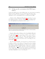
C.2 Setting up the environment (Qt SDK Opensource) . . . . . . 138
C.3 Main Software - Game software . . . . . . . . . . . . . . . . . 140
D Datasheet
143
VIII
List of Figures
2.1
2.2
2.3
2.4
2.5
2.6
2.7
2.8
The standard wheel and castor wheel . . . . .
Omniwheels . . . . . . . . . . . . . . . . . . .
Spherical Wheels . . . . . . . . . . . . . . . .
Differential drive configuration . . . . . . . .
Tri-cycle drive, combined steering and driving
MRV4 robot with synchro drive mechanism .
Palm Pilot Robot with omniwheels . . . . . .
Robots developed for games and interactions
3.1
3.2
3.3
3.4
3.5
3.6
3.7
3.8
3.9
3.10
3.11
3.12
3.13
3.14
3.15
3.16
The design of robot using Google SketchUp . . . . . . . . . .
The optimal torque / speed curve . . . . . . . . . . . . . . .
The calculated curve for the Pololu . . . . . . . . . . . . . . .
Pololu 25:1 Metal Gearmotor 20Dx44L mm. . . . . . . . . . .
The connection between the motors, chassis and wheels . . .
Wheels . . . . . . . . . . . . . . . . . . . . . . . . . . . . . . .
The wheel holder . . . . . . . . . . . . . . . . . . . . . . . . .
Three wheel configuration . . . . . . . . . . . . . . . . . . . .
The position of the camera . . . . . . . . . . . . . . . . . . .
The real camera position . . . . . . . . . . . . . . . . . . . . .
Bumpers . . . . . . . . . . . . . . . . . . . . . . . . . . . . . .
The bumper design . . . . . . . . . . . . . . . . . . . . . . . .
Robot with foams, springs and bumpers . . . . . . . . . . . .
J.tronik Li-Po Battery . . . . . . . . . . . . . . . . . . . . . .
Structure of an H bridge (highlighted in red) . . . . . . . . .
The schematics of voltage divider and voltage regulator circuit
22
24
25
26
26
27
28
29
30
30
31
32
32
33
35
37
4.1
4.2
4.3
4.4
The wheel position and robot orientation . . . . .
A linear movement . . . . . . . . . . . . . . . . . .
The angular movement calculated by simulator . .
The mixed angular and linear movement calculated
41
43
44
45
IX
.
.
.
.
.
.
.
.
.
.
.
.
.
.
.
.
.
.
.
.
.
.
.
.
.
.
.
.
.
.
.
.
.
.
.
.
.
.
.
.
.
.
.
.
.
.
.
.
.
.
.
.
.
.
.
.
.
.
.
.
.
.
.
.
.
.
.
.
.
.
.
.
.
.
.
.
.
.
.
.
.
.
.
.
.
.
.
.
.
.
.
.
.
.
.
.
6
7
7
9
9
10
11
18
5.1
5.2
5.3
5.4
5.5
5.6
5.7
.
.
.
.
.
.
.
52
54
55
62
63
63
64
A.1 The class diagram of the most used classes . . . . . . . . . . .
A.2 The flow diagram of the game algorithm . . . . . . . . . . . .
82
83
C.1
C.2
C.3
C.4
C.5
C.6
C.7
C.8
The images used in the camera calibration
Perspective projection in a pinhole camera
Camera robot world space . . . . . . . . .
Sample object . . . . . . . . . . . . . . . .
The histogram for each color channel . . .
The mask for each channel . . . . . . . . .
The mask applied to the orginal picture. .
The
The
The
The
The
The
The
The
.
.
.
.
.
.
.
.
.
.
.
.
.
.
.
.
.
.
.
.
.
.
.
.
.
.
.
.
.
.
.
.
.
.
.
.
.
.
.
.
.
.
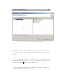
import screen of Eclipse . . . . . . . . . . . . .
import screen for Launch Configurations . . . .
second step at importing Launch Configurations
error Qt libraries not found . . . . . . . . . . .
drivers can be validated from Device Manager .
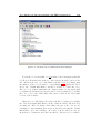
main screen of the ST’s software . . . . . . . . .
second step at importing Launch Configurations
programming of the microprocessor . . . . . . .
.
.
.
.
.
.
.
.
.
.
.
.
.
.
.
.
.
.
.
.
.
.
.
.
.
.
.
.
.
.
.
.
.
.
.
.
.
.
.
.
.
.
.
.
.
.
.
.
.
.
.
.
.
.
.
.
.
.
.
.
.
.
.
.
.
.
.
.
136
136
137
138
139
140
141
142
D.1 The schematics for the RVS Module board . . . . . . . . . . . 144
D.2 The schematics for the STL Mainboard . . . . . . . . . . . . 145
D.3 The pin-mappings of the board . . . . . . . . . . . . . . . . . 146
Chapter 1
Introduction
1.1
Goals
The aim of this thesis is to develop an autonomous robot implementing the
main functionalities needed for low-cost, but interesting robogames. There
are some predefined constraints for the robot. One of the most important
property is being the lowest cost possible. We limit the maximum cost to
250 euro. In order to satisfy this constraint, we focused on producing and
reusing some of the components or choosing the components that barely
work. Another constraint is the target environment of the robot, which is
home environment. The size and the weight of the robot have been chosen
in a way that it can move easily in home environments. The choice of the
kinematics and the wheels are made according to these needs.
1.2
Context, Motivations
Finding solutions for building robots capable of moving in home environment and to cooperate with people is a subject of much study prevalent in
recent years; many companies are investing in this area with the conviction
that, in the near future, robotics will represent an interesting markets.
The aim of this work has been to design and implement a home-based
mobile robot able to move at home and interacting with users involved in
games. The presented work concerns the entire development process, from
building a model of the system and the design of the chassis, mechanical
components and electronics needed for implementation robot control and
the acquisition of sensory data, up to the development of behaviors.
2
Chapter 1. Introduction
The preliminary phase of the project has been to study the kinematics
problem, which led to the creation of a model system to analyze the relationship between applied forces and motion of the robot.
The work proceeded with the design of mechanical parts, using solutions
to meet the needs of system modularity and using standard components as
much as possible. After modeling the chassis of the robot, and having selected the wheels, the actuators have been chosen.
The hardware design has affected the choice of sensors used for estimating the state of the system, and the design of a microcontroller-based control
logic.
The last part of the work consisted in carrying out experiments to estimate the position of the robot using the data from the sensors and to
improve the performance of the control algorithm. The various contributors
affecting the performance of the robot behavior have been tested, allowing
to observe differences in performance, and alternative solutions have been
implemented to cope with limitations due to low cost of HW and low computational power.
1.3
Achievements
We have been able to develop a robot that is able to follow successfully a
predefined colored object, thus implementing many interesting capabilities
useful for robogames. We have faced some limitations due to the low-cost
constraints. The main challenges have been caused by the absence of motor
encoders and low-cost optics. We have done some optimizations and tunings
to overcome these limitations.
1.4
Thesis Structure
The rest of the thesis is structured as follows: In chapter 2 we present the
state of the art, which is concentrated on similar applications, the techniques used, and what has been done previously. Chapter 3 is about the
mechanical construction and hardware architectures. Chapter 4 is the de-
1.4. Thesis Structure
3
tailed description of the control, what is necessary to replicate the same
work. Chapter 5 is the vision system description in detail, what has been
done, which approaches are used, and the implementation. Chapter 6 concerns game design for the tests made and the evaluation of the game results.
Chapter 7 concludes the presentation.
4
Chapter 1. Introduction
Chapter 2
State of the Art
Advances in computer engineering artificial intelligence, and high–tech
evolutions from electronics and mechanics have led to breakthroughs in
robotic technology [23]. Today, autonomous mobile robots can track a person’s location, provide contextually appropriate information, and act in response to spoken commands.
Robotics has been involved in human lives from industry domain to daily
life applications such as home helper or, recently, entertainment robots. The
latter introduced a new aspect of robotics, entertainment, which is intended
to make humans enjoy their lives from a various kind of view-points quite
different from industrial applications [17].
Interaction with robot is thought of a relatively new field, but the idea
of building lifelike machines that entertain people has fascinated us for hundreds of years since the first ancient mechanical automaton. Up to our days,
there have been major improvements in the development of robots.
We will review the literature for the robots that are related with our design. We divided the review in subsections like Locomotion, Motion Models,
Navigation, and Interaction and Games.
2.1
Locomotion
There exists a great variety of possible ways to move a robot, which makes
the selection of a robot’s approach to motion an important aspect of mobile
robot design. The most important of these are wheels, tracks and legs [33].
6
Chapter 2. State of the Art
The wheel has been by far the most popular motion mechanism in mobile robotics. It can achieve very good efficiency, with a relatively simple
mechanical implementation and construction easiness. On the other hand,
legs and tracks require complex mechanics, more power, and heavier hardware for the same payload. It is suitable to choose wheels for robot that is
designed to work in home environment, where it has to move mainly on a
plain surface.
There are three major wheel classes. They differ widely in their kinematics, and therefore the choice of wheel type has a large effect on the overall
kinematics of the mobile robot. The choice of wheel types for a mobile robot
is strongly linked to the choice of wheel arrangement, or wheel geometry.
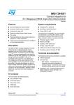
First of all there is the standard wheel as shown in Figure 2.1(a). The
standard wheel has a roll axis parallel to the plane of the floor and can
change orientation by rotating about an axis normal to the ground through
the contact point. The standard wheel has two DOF. The caster offset
standard wheel, also know as the castor wheel shown in Figure 2.1(b), has
a rotational link with a vertical steer axis skew to the roll axis. The key
difference between the fixed wheel and the castor wheel is that the fixed
wheel can accomplish a steering motion with no side effects, as the center
of rotation passes through the contact patch with the ground, whereas the
castor wheel rotates around an offset axis, causing a force to be imparted to
the robot chassis during steering [30].
(a) Standard Wheel
(b) Castor Wheel
Figure 2.1: The standard wheel and castor wheel
The second type of wheel is the omnidirectional wheel (Figure 2.2). The
omnidirectional wheel has three DOF and functions as a normal wheel, but
2.1. Locomotion
7
provides low resistance along the direction perpendicular to the roller direction as well. The small rollers attached around the circumference of the
wheel are passive and the wheel’s primary axis serves as the only actively
powered joint. The key advantage of this design is that, although the wheel
rotation is powered only along one principal axis, the wheel can kinematically move with very little friction along many possible trajectories, not just
forward and backward.
Figure 2.2: Omniwheels
The third type of wheel is the ball or spherical wheel in Figure 2.3. It
has also three DOF. The spherical wheel is a truly omnidirectional wheel,
often designed so that it may be actively powered to spin along any direction. There have not been many attempts to build a mobile robot with ball
wheels because of the difficulties in confining and powering a sphere. One
mechanism for implementing this spherical design imitates the first computer mouse, providing actively powered rollers that rest against the top
surface of the sphere and impart rotational force.
Figure 2.3: Spherical Wheels
The wheel type and wheel configuration are of tremendous importance,
8
Chapter 2. State of the Art
they form an inseparable relation and they influence three fundamental characteristics of a: maneuverability, controllability, and stability. In general,
there is an inverse correlation between controllability and maneuverability.
The number of wheels is the first decision. Two, three and four wheels
are the most commonly used each one with different advantages and disadvantages. The two wheels drive has very simple control but reduced maneuverability. The three wheels drive has simple control and steering but
limited traction. The four wheels drive has more complex mechanics and
control, but higher traction [38].
The differential drive is a two-wheeled drive system with independent
actuators for each wheel. The motion vector of the robot is the sum of the
independent wheel motions. The drive wheels are usually placed on each
side of the robot. A non driven wheel, often a castor wheel, forms a tripodlike support structure for the body of the robot. Unfortunately, castors can
cause problems if the robot reverses its direction. The castor wheel must
turn half a circle and, the offset swivel can impart an undesired motion vector to the robot. This may result in to a translation heading error. Straight
line motion is accomplished by turning the drive wheels at the same rate in
the same direction. In place rotation is done by turning the drive wheels at
the same rate in the opposite direction. Arbitrary motion paths can be implemented by dynamically modifying the angular velocity and/or direction
of the drive wheels. The benefits of this wheel configuration is its simplicity.
A differential drive system needs only two motors, one for each drive
wheel. Often the wheel is directly connected to the motor with internal
gear reduction. Despite its simplicity, the controllability is rather difficult,
especially to make a differential drive robot move in a straight line. Since
the drive wheels are independent, if they are not turning at exactly the
same rate the robot will veer to one side. Making the drive motors turn at
the same rate is a challenge due to slight differences in the motors, friction
differences in the drive trains, and friction differences in the wheel-ground
interface. To ensure that the robot is traveling in a straight line, it may be
necessary to adjust the motor speed very often. It is also very important to
have accurate information on wheel position. This usually comes from the
encoders. A round shaped differential drive configuration is shown in Figure
2.4.
In a tricycle vehicle (Figure 2.5) there are two fixed wheels mounted
2.1. Locomotion
9
Figure 2.4: Differential drive configuration with two drive wheels and a castor wheel
on a rear axle and a steerable wheel in front. The fixed wheels are driven
by a single motor which controls their traction, while the steerable wheel
is driven by another motor which changes its orientation, acting then as a
steering device. Alternatively, the two rear wheels may be passive and the
front wheel may provide traction as well as steering.
Figure 2.5: Tri-cycle drive, combined steering and driving
Another three wheel configuration is the synchro drive. The synchro
drive system is a two motor drive configuration where one motor rotates all
wheels together to produce motion and the other motor turns all wheels to
change direction. Using separate motors for translation and wheel rotation
guarantees straight line translation when the rotation is not actuated. This
mechanical guarantee of straight line motion is a big advantage over the
differential drive method where two motors must be dynamically controlled
to produce straight line motion. Arbitrary motion paths can be done by
actuating both motors simultaneously. The mechanism which permits all
wheels to be driven by one motor and turned by another motor is fairly
10
Chapter 2. State of the Art
complex. Wheel alignment is critical in this drive system, if the wheels are
not parallel, the robot will not translate in a straight line. Figure 2.6 shows
MRV4 a robot with this drive mechanism.
Figure 2.6: MRV4 robot with synchro drive mechanism
The car type locomotion or Ackerman steering configuration is used in
cars. The limited maneuverability of Ackerman steering has an important
advantage: its directionality and steering geometry provide it with very
good lateral stability in high-speed turns. The path planning is much more
difficult. Note that the difficulty of planning the system is relative to the
environment. On a highway, path planning is easy because the motion is
mostly forward with no absolute movement in the direction for which there
is no direct actuation. However, if the environment requires motion in the
direction for which there is no direct actuation, path planning is very hard.
Ackerman steering is characterized by a pair of driving wheels and a separate
pair of steering wheels. A car type drive is one of the simplest locomotion
systems in which separate motors control translation and turning this is a
big advantage compared to the differential drive system. There is one condition: the turning mechanism must be precisely controlled. A small position
error in the turning mechanism can cause large odometry errors. This simplicity in line motion is why this type of locomotion is popular for human
driven vehicles.
Some robots are omnidirectional, meaning that they can move at any
time in any direction along the ground plane (x, y) regardless of the orientation of the robot around its vertical axis. This level of maneuverability requires omnidirectional wheels which present manufacturing challenges.
Omnidirectional movement is of great interest to complete maneuverability.
2.1. Locomotion
11
Omnidirectional robots that are able to move in any direction (x, y, θ) at
any time are also holonomic. There are two possible omnidirectional configurations.
The first omnidirectional wheel configuration has three omniwheels, each
actuated by one motor, and they are placed in an equilateral triangle as depicted in Figure 2.7. This concept provides excellent maneuverability and is
simple in design, however, it is limited to flat surfaces and small loads, and
it is quite difficult to find round wheels with high friction coefficients. In
general, the ground clearance of robots with Swedish and spherical wheels
is somewhat limited due to the mechanical constraints of constructing omnidirectional wheels.
Figure 2.7: Palm Pilot Robot with omniwheels
The second omnidirectional wheel configuration has four omniwheel each
driven by a separate motor. By varying the direction of rotation and relative
speeds of the four wheels, the robot can be moved along any trajectory in
the plane and, even more impressively, can simultaneously spin around its
vertical axis. For example, when all four wheels spin ’forward’ the robot as
a whole moves in a straight line forward. However, when one diagonal pair
of wheels is spun in the same direction and the other diagonal pair is spun
in the opposite direction, the robot moves laterally. These omnidirectional
wheel arrangements are not minimal in terms of control motors. Even with
all the benefits, few holonomic robots have been used by researchers because
of the problems introduced by the complexity of the mechanical design and
controllability.
In mobile robotics the terms omnidirectional, holonomic and non holonomic are often used, a discussion of their use will be helpful. Omnidirectional simply means the ability to move in any direction. Because of the
planar nature of mobile robots, the operational space they occupy contains
12
Chapter 2. State of the Art
only three dimensions which are most commonly thought of as the x, y
global position of a point on the robot and the global orientation, θ, of the
robot. A non holonomic mobile robot has the following properties:
• The robot configuration is described by more than three coordinates.
Three values are needed to describe the location and orientation of the
robot, while others are needed to describe the internal geometry.
• The robot has two DOF, or three DOF with singularities.
A holonomic mobile robot has the following properties:
• The robot configuration is described by three coordinates. The internal geometry does not appear in the kinematic equations of the robot,
so it can be ignored.
• The robot has three DOF without singularities.
• The robot can instantly develop a force in an arbitrary combination
of directions x, y, θ.
• The robot can instantly accelerate in an arbitrary combination of directions x, y, θ.
Non holonomic robots are most common because of their simple design
and ease of control. By their nature, non holonomic mobile robots have
fewer degrees of freedom than holonomic mobile robots. These few actuated
degrees of freedom in non holonomic mobile robots are often either independently controllable or mechanically decoupled, further simplifying the
low-level control of the robot. Since they have fewer degrees of freedom,
there are certain motions they cannot perform. This creates difficult problems for motion planning and implementation of reactive behaviors.
However, holonomic offer full mobility with the same number of degrees of
freedom as the environment. This makes path planning easier because there
are no constraints that need to be integrated. Implementing reactive behaviors is easy because there are no constraints which limit the directions
in which the robot can accelerate.
2.2. Motion Models
2.2
13
Motion Models
In the field of robotics the topic of robot motion has been studied in depth
in the past. Robot motion models play an important role in modern robotic
algorithms. The main goal of a motion model is to capture the relationship between a control input to the robot and a change in the robot’s pose.
Good models will capture not only systematic errors, such as a tendency of
the robot to drift left or right when directed to move forward, but will also
capture the stochastic nature of the motion. The same control inputs will
almost never produce the same results and the effects of robot actions are,
therefore, best described as distributions [41]. Borenstein et al. [32] cover
a variety of drive models, including differential drive, the Ackerman drive,
and synchro-drive.
Previous work in robot motion models have included work in automatic
acquisition of motion models for mobile robots. Borenstein and Feng [31]
describe a method for calibrating odometry to account for systematic errors. Roy and Thrun [41] propose a method which is more amenable to
the problems of localization and SLAM. They treat the systematic errors
in turning and movement as independent, and compute these errors for
each time step by comparing the odometric readings with the pose estimate
given by a localization method. Alternately, instead of merely learning two
simple parameters for the motion model, Eliazat and Parr [15] seek to use
a more general model which incorporates interdependence between motion
terms, including the influence of turns on lateral movement, and vice-versa.
Martinelli et al. [16] propose a method to estimate both systematic and
non-systematic odometry error of a mobile robot by including the parameters characterizing the non-systematic error with the state to be estimated.
While the majority of prior research has focused on formulating the pose estimation problem in the Cartesian space. Aidala and Hammel [29], among
others, have also explored the use of modified polar coordinates to solve
the relative bearing-only tracking problem. Funiak et al. [40] propose an
over-parameterized version of the polar parameterization for the problem
of target tracking with unknown camera locations. Djugash et al. [24] further extend this parameterization to deal with range-only measurements
and multimodal distributions and further extend this parameterization to
improve the accuracy of estimating the uncertainty in the motion rather
than the measurement.
14
2.3
Chapter 2. State of the Art
Navigation
A navigation environment is in general dynamic. Navigation of autonomous
mobile robots in an unknown and unpredictable environment is a challenging
task compared to the path planning in a regular and static terrain, because
it exhibits a number of distinctive features. Environments can be classified
as known environments, when the motion can be planned beforehand, or
partially known environments, when there are uncertainties that call for a
certain type of on-line planning for the trajectories. When the robot navigates from original configuration to goal configuration through unknown
environment without any prior description of the environment, it obtains
workspace information locally while it is moving and a path must be incrementally computed as the newer parts of the environment are explored [26].
Autonomous navigation is associated to the capability of capturing information from the surrounding environment through sensors, such as vision,
distance or proximity sensors. Even though the fact that distance sensors,
such as ultrasonic and laser sensors, are the most commonly used ones, vision
sensors are becoming widely applied because of its ever-growing capability
to capture information at low cost.
Visual control methods fall into three categories such as position based,
image based and hybrid [28]. The position based visual control method reconstructs the object in 3D space from 2D image space, and then computes
the errors in Cartesian space. For example, Han et al [25] presented a position based control method to open a door with a mobile manipulator, which
calculated the errors between the end-effector and the doorknob in Cartesian space using special rectangle marks attached on the end-effector and
doorknob. As Hager [28] pointed out, the position based control method has
the disadvantage of low precision in positioning and control. To improve the
precision, El-Hakim et al [39] proposed a visual positioning method with 8
cameras, in which the positioning accuracy was increased through iteration.
It has high positioning accuracy but poor performance in real time.
The image based visual control method does not need to reconstruct
in 3D space, but the image Jacobian matrix needs to be estimated. The
controller design is difficult. And the singular problem in image Jacobian
matrix limits its application [28]. Hybrid control method attempts to give a
good solution through the combination of position and image based visual
control methods. It controls the pose with position based method, and the
position with image based method. For example, Malis et al [35] provided
2.4. Games and Interaction
15
a 2.5 D visual control method. Deguchi et al. [22] proposed a decoupling
method of translation and rotation. Camera calibration is a tedious task,
and pre-calibration cameras used in visual control methods limit a lot the
flexibility of the system. Therefore, many researchers pursue the visual
control methods with self-calibrated or un-calibrated cameras. Kragic et
al. [34] gave an example to self-calibrate a camera with the image and the
CAD model of the object in their visual control system. Many researchers
proposed various visual control methods with un-calibrated cameras, which
belong to image based visual control methods. The camera parameters are
not estimated individually, but combined into the image Jacobian matrix.
For instance, Shen et al. [43] limited the working space of the end-effector
on a plane vertical to the optical axis of the camera to eliminate the camera
parameters in the image Jacobian matrix. Xu et al. [21] developed visual
control method for the end-effector of the robot with two un-calibrated cameras, estimating the distances based on cross ratio invariance.
2.4
Games and Interaction
Advances in the technological medium of video games have recently included
the deployment of physical activity-based controller technologies, such as the
Wii [27], and vision-based controller systems, such as Intel’s Me2Cam [13].
The rapid deployment of millions of iRobot Roomba home robots [14] and
the great popularity of robotic play systems, such as LEGO Mindstorms
and NXT [5] now present an opportunity to extend the realm of video game
even further, into physical environments, through the direct integration of
human-robot interaction techniques and architectures with video game experiences.
Over the past thirty to forty years, a synergistic evolution of robotic
and video game-like programming environments, such as Turtle Logo [36],
has occurred. At the MIT Media Lab, these platforms have been advanced
through the constructionist pedagogies, research, and collaborations of Seymour Papert, Marvin Minsky, Mitch Resnick, and their colleagues, leading
to Logo [7], Star Logo [37], programmable Crickets and Scratch [6] and Lego
MindStorms [37]. In 2000, Kids Room [18] demonstrated that an immersive
educational gaming environment with projected objects and characters in
physical spaces (e.g., on the floor or walls), could involve children in highly
interactive games, such as hide-and-seek. In 2004, RoBallet [20] advanced
these constructionist activities further, blending elements of projected vir-
16
Chapter 2. State of the Art
tual environments with sensor systems that reacted to children dancing in
a mediated physical environment. The realm of toys and robotic pets has
also seen the development of a wide array of interactive technologies (e.g.,
Furby, Aibo, Tamagotchi) and more recently Microsoft’s Barney [9], which
has been integrated with TV-based video content. Interactive robotic environments for education are now being extended to on-line environments,
such as CMU’s educational Mars rover [8], and becoming popular through
robotics challenges such as FIRST Robotics Competition [3], BattleBots [1],
and Robot World Cup soccer tournaments, such as Robocup [42].
The games related with robots, so called robogames, are categorized
into four branches according to AIRLab report [19]. One is the videogames,
where robot characters are simulated. Soccer Simulation League in RoboCupSoccer is an example of this kind of games. The Simulation League focuses
on artificial intelligence and team strategy. Independently moving software
players (agents) play soccer on a virtual field inside a computer. This provides a context to the game, but also allows to escape all the limitations
of physical robots. Another one is the tele-operated physical robots, where
the player is mainly in the manipulation of remote controllers similar to the
ones used in videogames, or, eventually, in the physical building of the teleoperated robots, as it happens with RoboWars [11]. A third main stream
concerns robots that have been developed by roboticists to autonomously
play games (e.g., Robocup). Here, the accent is on the ability to program
the robots to be autonomous, but little effort is spent in the eventual playful
interaction with people, often avoided, as in most of the Robocup leagues.
The last main stream concerns robots that act as more or less like mobile
pets. In this case, interaction is often limited to almost static positions, not
exploiting rich movement, nor high autonomy; the credibility of these toys
to really engage healthy people, such as kids, is not high.
According to the AIRLab report [19], a new category of games where
the players are involved in a challenging and highly interactive game activity with autonomous robots called as Highly Interactive, Competitive
RoboGames (HI-CoRG) is introduced. The idea is to take the videogame
players away from screen and console, and to make them physically interact
with a robot in their living environment. In this context some heuristics
from videogames adapted to be applied on this HI-CoRG games.
In our thesis, we focused on developing a robot for games that can be
count to the HI-CoRG category.
2.4. Games and Interaction
17
We introduce now some of the robots developed in the past, related to
the human robot interaction and games.
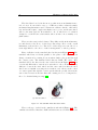
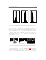
Kismet (Figure 2.8(a)) is a robot made in the late 1990s at Massachusetts
Institute of Technology with auditory, visual and expressive systems intended to participate in human social interaction and to demonstrate simulated human emotion and appearance. This project focuses not on robotrobot interactions, but rather on the construction of robots that engage
in meaningful social exchanges with humans. By doing so, it is possible
to have a socially sophisticated human assist the robot in acquiring more
sophisticated communication skills and helping it to learn the meaning of
these social exchanges.
A Furby (Figure 2.8(b)) was a popular electronic robotic toy resembling
a hamster/owl-like creature which went through in 1998. Furbies were the
first successful attempt to produce and sell a domestically-aimed robot. A
newly purchased Furby starts out speaking entirely Furbish, the unique language that all Furbies use, but are programmed to speak less Furbish as
they gradually start using English. English is learned automatically, and
no matter what culture they are nurtured in, they learn English. In 2005,
new Furbies were released, with voice-recognition and more complex facial
movements, and many other changes and improvements.
AIBO (Artificial Intelligence Robot) (Figure 2.8(c)) was one of several
types of robotic pets designed and manufactured by Sony. There have been
several different models since their introduction on May 11, 1999. AIBO is
able to walk, ”see” its environment via camera and recognize spoken commands in Spanish and English. AIBO robotic pets are considered to be
autonomous robots since they are able to learn and mature based on external stimuli from their owner, their environment and from other AIBOs.
The AIBO has seen use as an inexpensive platform for artificial intelligence
research, because it integrates a computer, vision system, and articulators in
a package vastly cheaper than conventional research robots. The RoboCup
autonomous soccer competition had a ”RoboCup Four-Legged Robot Soccer League” in which numerous institutions from around the world would
participated. Competitors would program a team of AIBO robots to play
games of autonomous robot soccer against other competing teams.
The developments in Robocup lead to improvements in the mobile robots.
18
Chapter 2. State of the Art
(a) Kismet
(b) Furby
(d) Spykee
(c) AIBO
(e) Rovio
Figure 2.8: Robots developed for games and interactions
The domestically-aimed robots become popular in the market. One of them
is Spykee (Figure 2.8(d)), which is a robotic toy made by Meccano in 2008.
It contains a USB webcam, microphone and speakers. Controlled by computer locally or over the internet, the owner can move the robot to various
locations within range of the local router, take pictures and video, listen to
surroundings with the on-board microphone and play sounds/music or various built-in recordings (Robot laugh, laser guns, etc.) through the speaker.
Spykee has a WiFi connectivity to let him access the Internet using both
ad-hoc and infrastructure modes.
Similar to Spykee, with different kinematics models and more improvements, RovioTM (Figure 2.8(e)) is the groundbreaking new Wi-Fi enabled
mobile webcam that views and interacts with its environment through video
and audio streaming.
According to our goals, we investigated the previously made robots, since
we thought we could benefit from the techniques used. Furbies have expressions, but they don’t move. While Rovio has omnidirectional, Spykee has
tracks for the motion, but they lack entertainment. AIBO has legs and a
2.4. Games and Interaction
19
lot of motors, but these brings more cost and high complexity for the development.
20
Chapter 2. State of the Art
Chapter 3
Mechanical Construction
We started our design from these specifications of the robot.
• a dimension of about 25 cm of radius, 20 cm height
• a speed of about 1 m/sec
• sensors to avoid obstacles
• a camera that can be moved up and down
• power enough to move and transmit for at least 2 hours without
recharging
• the robot should cost no more than 250 euro.
In the development process we faced some problems due to the limitations from the specifications. Main causes of these problems are related with
low-cost, that is coming with our design constraints.
The mechanical construction of the robot is focused on construction
of the robot chassis, motor holders, motor and wheel connections, camera
holder, the foam covering the robot, batteries and hardware architectures.
3.1
Chassis
The main principles for the construction of the chassis are coming from
similar projects from the past, which are the simplicity of assembly and
disassembly, the ease of access to the interior and the possibility of adding
22
Chapter 3. Mechanical Construction
and modifying elements in the future. We decided to use some design constraints, revising these according to our goals.
The design is started with the choice of the chassis made of plexiglas.
One advantage of using plexiglas, it is 43% lighter than aluminum [10]. Another advantage that is affecting our choice is the electrical resistance of the
plexiglas, that will isolate any accidental short circuit. One of the major
problems with plexiglas is the difficult processing of the material. However,
it has to be processed only once, hence this is negligible.
Figure 3.1: The design of robot using Google SketchUp
The preliminary design has been created with Google SketchUp, allowing to define the dimensions of the robot and the arrangement of various
elements shown in Figure 3.1. This model has been used to obtain a description of the dynamics of the system. The robot is 125 mm in diameter wide
and 40 cm in height, meeting the specification to be contained in a footprint
on the ground in order to move with agility in the home. The space between
the two plates is around 6 cm, which allows us to mount sensors and any
device that will be added in the future. The total weight of the structure is
approximately 1.8 kg, including motors and batteries.
3.2. Motors
23
The initial design of the chassis was a bit different from the final configuration seen in Figure 3.1. Even though the shape of the components did not
change, the position and orientation are changed in the final configuration.
The motor holders initially were intended to be placed on the top of the
bottom plexiglas layer. At the time when this decision was taken, we were
not planning to place the mice boards, but only to put the batteries and the
motor control boards. Later, with the decision of placing the mice boards in
this layer, in order to get more space, we decided to put the motors to their
final position. So this configuration increases the free space on the robot
layers to put the components, and also increases the robot height from the
ground that will result to better navigation.
Another change has been made by placing the second plexiglas layer.
Initially, we placed that layer using only three screws with each a height of
6 cm. The idea was using minimum screws, so that the final weight will
be lighter and the plexiglas will be more resistant to damage. Later, when
we placed the batteries, motor controller boards and the camera with its
holder, the total weight was too much to be handled by the three screws.
And additionally, we placed 6 more screws with the same height as before.
These screws, allowed us to divide the total weight on the plate equally on
all the screws and also enabled us to install springs and foams, to implement
bumpers that protect the robot from any damage that could be caused by
hits.
3.2
Motors
The actuator is one of the key components in the robot. Among the possible
actuation we decided to go with DC motors. Servo motors are not powerful
enough to reach the maximum speed. Due to noise and control circuitry
requirements, servos are less efficient than uncontrolled DC motors. The
control circuitry typically drains 5-8mA on idle. Secondly, noise can draw
more than triple current during a holding position (not moving), and almost
double current during rotation. Noise is often a major source of servo inefficiency and therefore they should be avoided. Brushless motors are more
power efficient, have a significantly reduced electrical noise, and last much
longer. However, they also have several disadvantages, such as higher price
and the requirement for a special brushless motor driver. Since they are
running at high speed we need to gear them down. This would also add
24
Chapter 3. Mechanical Construction
some extra cost. Also the Electronic Speed Controllers(ESC) are costly and
most of them do not support multiple run motors. The minimum price for
the motor is about 20 dollars, and for the ESC is around 30 dollars. The
minimum expected price for motors and controller will be a least 90 dollars
if we can run the 3 motors on a single controller. Also there should be an
extra cost to gear them down.
We made some calculations to find the most suitable DC motor for our
system. In order to effectively design with DC motors, it is necessary to
understand their characteristic curves. For every motor, there is a specific
torque/speed curve and power curve. The graph in Figure 3.2 shows a
torque/speed curve of a typical DC motor.
Figure 3.2: The optimal torque / speed curve
Note that, torque is inversely proportional to the speed of the output
shaft. In other words, there is a trade-off between how much torque a motor
delivers, and how fast the output shaft spins. Motor characteristics are
frequently given as two points:
• The stall torque, τs , represents the point on the graph at which the
torque is a maximum, but the shaft is not rotating.
• The no load speed, ωn , is the maximum output speed of the motor
(when no torque is applied to the output shaft).
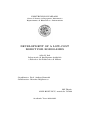
The linear model of a DC motor torque/speed curve is a very good approximation. The torque/speed curves shown below in Figure 3.3 are calculated curves for our motor, which is Pololu 25:1 Metal Gearmotor 20Dx44L
mm.
3.2. Motors
25
Figure 3.3: The calculated curve for the Pololu 25:1 Metal Gearmotor 20Dx44L mm
Due to the linear inverse relationship between torque and speed, the
maximum power occurs at the point where ω = 12 ωn , and τ = 21 τs . The
maximum power output occuring at no load speed with, τ = 500rpm =
52.38rad/sec, and the stall torque, ω = 0.282N m is calculated as follows:
P =τ ∗ω
1
1
P max = τs ∗ ωn
2
2
P max = 26.190rad/sec ∗ 0.141N m = 3.692W
Keeping in mind the battery life, the power consumption, the necessary
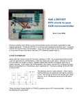
torque and the maximum speed, we selected the Pololu motors shown in
Figure 3.4.
In the design of the robot we decided to use low cost components. In
that sense we focused on producing components or re-using components that
can be modified according to our demands. The mechanical production of
the components took some time both for the design and the construction
process (e.g. the connectors between motors and wheels are milled from an
aluminum bar), however this reduced the overall cost. The connection of
motors with robot is made by putting the motor inside an aluminum tube,
merging it with the U-shaped plate (Figure 3.5). Using such a setup helps
26
Chapter 3. Mechanical Construction
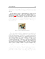
Figure 3.4: Pololu 25:1 Metal Gearmotor 20Dx44L mm. Key specs at 6 V: 500 RPM
and 250 mA free-run, 20 oz-in (1.5 kg-cm) and 3.3 A stall.
not only protecting the motor from the hit damage, but also cooling of the
motor since aluminum has great energy-absorbing characteristics [12]. The
connection can be seen clearly in Figure 3.5. The component is attached to
the plexiglas from the L-shaped part using a single screw. This gives us the
flexibility to dis-attach the component easily and to change the orientations
of them if needed.
Figure 3.5: The connection between the motors, chassis and wheels
3.3
Wheels
The target environment of our robot is a standard home. The characteristic properties of this environment that are important for our work are as
follows. Mainly the environment is formed by planes, surfaces such as parquet, tile, carpet etc... In order to move freely to any direction on these
surfaces and reach the predefined speed constraint, we selected the wheels
and a proper configuration for them. The decision to choose omnidirectional
wheel was motivated, but there are lots of different omnidirectional wheels
available on the market. Among them, we made a selection considering the
3.3. Wheels
27
target surface, maximum payload, weights of the wheels, and price. The
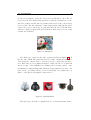
first selected wheel was the omniwheel shown in Figure 3.6(a). The wheel
consists of three small rollers, which may affect the turning since the coverage is not good enough. Also the wheel itself is heavier than the one with
the transwheel shown in Figure 3.6(b) A single transwheel is 0.5 oz lighter
than an omniwheel. Another model is the double transwheel seen in Figure
3.6(c), which is produced by merging two transwheels, where the rollers are
covering all the wheel, which will enable the movement in any direction easily and more consisting model by reducing the possible power transmission
loss that can be occur, when merging the two wheels by hand.
(a) Omniwheel
(b) Transwheel
(c) Double Transwheel
Figure 3.6: Wheels
In order reach the maximum speed of 1 m/sec., we should have the
following equation.
speed = circumref erence ∗ rps
speed = diameter ∗ pi ∗ rps
As it can be seen from the equation the speed is also related with the rotation per second (rps) of the wheels, which is determined by the motor. So
the dimension choice of the wheels are made keeping the rps in mind. The
rpm necessary to turn our wheels with the maximum speed of 1 meter/second the is calculated as follows:
1000mm/second = diameter ∗ pi ∗ rps
1000mm/second = 49.2mm ∗ pi ∗ rps
rps ∼
= 6.4
28
Chapter 3. Mechanical Construction
rpm ∼
= 388
As a result of the calculation, using the omniwheel with outer diameter
of 49.2 m., we will need a motor that can run around 388 rpm to reach the
maximum speed.
Figure 3.7: The wheel holder bar, that is making the transmission between motors and
wheels
The transmission between motors and wheels is achieved by the bar,
which is lathed from an aluminum bar (Figure 3.7). The bar is placed inside
the wheel and locked with a key using the key-ways in the wheel and the bar.
For the wheel configuration we preserved the popular three wheeled configuration (Figure 3.8). The control is simple, the maneuverability is enough
to satisfy the design specifications. The details of this configuration will be
mentioned in Control Chapter.
3.4
Camera
The camera positioning is tricky. We needed a holder that should be light in
the weight, but also provide enough height and width to enable vision from
the boundary of the robot at ground to the people face in the environment.
The initial tests have been made by introducing a camera holder using parts
from ITEM [4]. These parts are useful during the tests since they are easily
configurable for different orientations, and easy to assemble. But, the parts
are too heavy and we decided to use an aluminum bar for the final configuration. The movement of the camera is done by the servo placed at the top
of the aluminum bar; this gave us the flexibility to have different camera
3.5. Bumpers
29
Figure 3.8: Three wheel configuration
positions, that will be useful to develop different games.
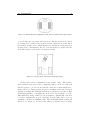
The camera is placed in a position on top of a mounted-on aluminum
bar that allows us to have the best depth of field by increasing the field
of view. The idea is to detect objects and visualize the environment between the boundary of the robot to all the way in the ground and up to
2 meters in height, which allows also to see faces of people or the objects
not on the ground. Mechanically, the camera itself is connected to a servo
that enables the camera head to move freely in 120◦ in the vertical axis, as
shown in Figure 3.9 and 3.10. This configuration gives us the flexibility to
generate different types of games using the vision available in a wide angle
and interchangeable height.
3.5
Bumpers
The last mechanical component is the collision detection mechanism, to
avoid obstacles in the environment. There are lots of good solutions to this
issue. By using different types of sensors such as sonars, photo resistors,
30
Chapter 3. Mechanical Construction
Figure 3.9: The position of the camera
Figure 3.10: The real camera position
IR sensors, tactile bumpers, etc. Among them, the simplest are the tactile
bumpers. A tactile bumper is probably one of the easiest way of letting a
robot know if it’s colliding with something. Indeed, they are implemented
by electrical switches. The simplest way to do this is to fix a micro switch to
robot in a way so that when it collides the switch will be pushed in, making
an electrical connection. Normally the switch will be held open by an internal spring. Tactile bumpers are great for collision detection, but the circuit
3.6. Batteries
31
itself also works fine for user buttons and switches as well. There are many
designs possible for bump switches, often depending on the design goals of
the robot itself. But the circuit remains the same. They usually implement
a mechanical button to short the circuit, pulling the signal line high or low.
An example is the micro switch with a lever attached to increase its range,
as shown in Figure 3.11. The cost is nothing if compared to the other solutions such as photo-resistors and sonars, and the usage is pretty simple since
the values can be read directly from the microcontroller pins without having
any control circuits. Major drawback is its limited range, but we tried to
improve the range using the foam and the external springs attached to the
foam. Since the robot is light in the weight and collision can be useful in
development of games, we decided to use tactile bumpers.
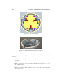
Figure 3.11: Bumpers are mechanical buttons to short the circuit, pulling the signal
line high or low.
The collision detection for robot is made with bumpers, which are placed
on the plexiglas every 60◦ (Figure 3.12). The coverage was not enough, so the
bumpers are covered with foams which are connected to the springs. The
springs are enabling the push back of the switches, the foams are increasing
the coverage of the collision detection and also enhance the safety both for
the damage that could be caused by the robot and to the robot from environment (Figure 3.13). After some tests we realized there are still dead
points which the collision are not detected. We decided to cut the foam into
three, placing the around the robot leaving the parts with the wheel open.
The best results are obtained using this configuration so we decided to keep
it.
3.6
Batteries
The robot’s battery life without the need of recharging is crucial for the
game. The game play must continue for about 2 hours without any interruption. This brings the question of how to choose the correct battery.
LiPo batteries are suitable battery choice for our application over conven-
32
Chapter 3. Mechanical Construction
Figure 3.12: The bumper design
Figure 3.13: Robot with foams, springs and bumpers
tional rechargeable battery types such as NiCad, or NiMH, for the following
reasons :
• LiPo batteries are light in weight and can be made in almost any shape
and size.
• LiPo batteries have large capacities, meaning they hold lots of power
in a small package.
• LiPo batteries have high discharge rates to power the most demanding
electric motors.
3.7. Hardware Architecture
33
In short, LiPo provide high energy storage to weight ratios in an endless
variety of shapes and sizes. The calculation is made to find the correct
battery. The motors are consuming 250 mA at free-run and 3300 mA for
the stall current. For the all three motors we should have the following
battery lives:
Battery Capacity/Current Draw = Battery Lif e
2 ∗ 2500mAh/750mA ∼
= 6.6hours
2 ∗ 2500mAh/9900mA ∼
= 0.5hours
using the 2 batteries each having a capacity of 2500 mAh. The battery
life shows changes according to the current draw of the motors. In case,
each motor is consuming 250 mA in free-run current will result 6.6 hours of
batteries life. On the other hand, with the stall current it will be 0.5 hour
battery life. Since the motor will not always work in stall current or the
free-run current; the choice of 2500 mA batteries (Figure 3.14) seems to be
enough to power the robot for at least 2 hours.
Figure 3.14: J.tronik - Battery Li-Po Li-POWER 2500 mA 2S1P 7,4V 20C
3.7
Hardware Architecture
During the development of the robot, we used several hardware pieces such
as microprocessor, camera, motor control boards, voltage regulator circuit,
voltage divider circuit. Most of them were already developed systems and
we did not focus on the production details of them. We only created the
voltage regulator and divider circuit, which we used in order to power the
boards and measure the battery level of charge.
34
Chapter 3. Mechanical Construction
The main component in our system is the the STL Main Board, known
also as STLCam. The STL Main Board is a low-cost vision system for acquisition and real-time processing of pictures, consisting of a ST-VS6724
Camera (2 Mpx), a ST-STR912FA Microcontroller (ARM966 @ 96MHz)
and 16MB of external RAM (PSRAM BURST). The schematics of the STL
Main Board is shown in Appendix D.2.
ST-STR912FAZ44 Microcontroller
The microcontroller main components are: a 32 bit ARM966E-S RISC
processor core running at 96MHz, a large 32bit SRAM (96KB) and a highspeed 544KB Flash memory. The ARM966E-S core can perform single-cycle
DSP instructions, good for speech recognition, audio and embedded vision
algorithms.
ST-VS6724 Camera Module
The VS6724 is a UXGA resolution CMOS imaging device designed for
low power systems, particularly mobile phone and PDA applications. Manufactured using ST 0.18µ CMOS Imaging process, it integrates a highsensitivity pixel array, digital image processor and camera control functions.
The device contains an embedded video processor and delivers fully color
processed images at up to 30 fps UXGA JPEG, or up to 30 fps SVGA YCbCr
4:2:2. The video data is output over an 8-bit parallel bus in JPEG (4:2:2 or
4:2:0), RGB, YCbCr or Bayer formats and the device is controlled via an I2C
interface. The VS6724 camera module uses ST’s second generation SmOP2
packaging technology: the sensor, lens and passives are assembled, tested
and focused in a fully automated process, allowing high volume and low cost
production. The VS6724 also includes a wide range of image enhancement
functions, designed to ensure high image quality, these include: automatic
exposure control, automatic white balance, lens shading compensation, defect correction algorithms, interpolation (Bayer to RGB conversion), color
space conversion, sharpening, gamma correction, flicker cancellation, NoRA
noise reduction algorithm, intelligent image scaling, special effects.
MC33887 Motor Driver Carrier
All electric motors need some sort of controller. The motor controller
may different features and complexity depending on the task that the motors will have to perform.
3.7. Hardware Architecture
35
The simplest case is a switch to connect a motor to a power source, such
as in small appliances or power tools. The switch may be manually operated
or may be a relay or conductor connected to some form of sensor to automatically start and stop the motor. The switch may have several positions
to select different connections of the motor. This may allow reduced-voltage
starting of the motor, reversing control or selection of multiple speeds. Overload and over-current protection may be omitted in very small motor controllers, which rely on the supplying circuit to have over-current protection.
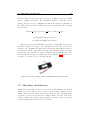
Figure 3.15: Structure of an H bridge (highlighted in red)
The DC motors cannot be controlled directly from the output pins of
the microcontroller. We need the circuit so called ’motor controller’, ’motor
driver’ or an ’H-Bridge’. The term H-Bridge is derived from the typical
graphical representation of such a circuit. An H-Bridge (Figure 3.15) is
built with four switches (solid-state or mechanical). When the switches S1
and S4 are closed (and S2 and S3 are open) a positive voltage will be applied across the motor. By opening S1 and S4 switches and closing S2 and
S3 switches, this voltage is reversed, allowing reverse operation of the motor.
To drive motors we used a PWM signal and vary the duty cycle to act
as a throttle: 100% duty cycle = full speed, 0% duty cycle = coast, 50%
duty cycle = half speed etc. After some testing we optimized the percentage
of the duty cycle in order achieve a better performance. This optimization
will be mentioned later in Control Chapter.
For the motor control, we started by using the H-Bridge motor control
circuits provided by our sponsor. The initial tests have been performed by
implementing the correct PWM waves using these boards. Later, we real-
36
Chapter 3. Mechanical Construction
ized that the boards were configured to work at 8 V. This forced us to make
the decision of buying new batteries or new control circuits. Evaluating the
prices, we ended up buying new control circuits that are rated for 5 V.
MC33887 motor driver integrated circuit is an easy solution to connect
a brushed DC motor running from 5 to 28 V and drawing up to 5 A (peak).
The board incorporates all the components of the typical application, plus
motor-direction LEDs and a FET for reverse battery protection. A microcontroller or other control circuit is necessary to turn the H-Bridge on and
off. The power connections are made on one end of the board, and the control connections (5V logic) are made on the other end. The enable (EN) pin
does not have a pull-up resistor, so it be must pulled to +5 V in order to
wake the chip from sleep mode. The fault-status (FS, active low) output pin
may be left disconnected if it is not needed to monitor the fault conditions of
the motor driver; if it is connected, it must use an external pull-up resistor
to pull the line high. IN1 and IN2 control the direction of the motor, and
D2 can be PWMed to control the motor’s speed. D2 is the ”not disabled“
line: it disables the motor driver when it is driven low (another way to think
of it is that, it enables the motor driver when driven high). Whenever D1
or D2 disable the motor driver, the FS pin will be driven low. The feedback
(FB) pin outputs a voltage proportional to the H-Bridge high-side current,
providing approximately 0.59 volts per amp of output current.
Voltage Divider and Voltage Regulator Circuit
Batteries are never at a constant voltage. For our case 7.2 V battery will
be at around 8.4 V when fully charged, and can drop to 5 V when drained.
In order to power microcontroller (and especially sensors) which are sensitive to the input voltage, and rated to 5 V, we need a voltage regulator
circuit to output always 5 V. The design of the circuit that will be used in
voltage regulation merged with the voltage divider circuit that will be used
for battery charge monitor shown in Figure 3.16.
To operate voltage divider circuit, the following equation is used to determine the appropriate resistor values.
Vo =
Vi
∗ R2
R1 + R2
Vi is the input voltage, R1 and R2 are the resistors, and Vo is the output
voltage.
3.7. Hardware Architecture
37
With the appropriate selection of resistor R1 and R2 based on the above
information, Vo will be suitable for the analog port on microcontroller. The
divider is used to input to the microcontroller a signal proportional to the
voltage provided by the battery, so to check its charge. Note that a fully
charged battery can often be up to 20% more of its rated value and a fully
discharged battery 20% below its rated value. For example, a 7.2 V battery
fully charged can be 8.4 V, and fully discharged 5 V. The voltage divider
circuit allows to read the battery level from the microcontroller pins directly,
that will be used in order to monitor battery charging level changes.
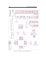
Figure 3.16: The schematics of voltage divider and voltage regulator circuit
From the Figure 3.16, the pin V out is used in order to monitor the battery life, which is placed on the left side of schematics. The divided voltage
is read from the analog input of the microcontroller. The voltage regulator
circuit which is placed on the right part of the schematics is used to power
the STLCam board with 5 V through the USB port. It can be also used in
order to make the connection with the PC, to transmit some data, which
we use for debug purposes.
38
Chapter 3. Mechanical Construction
Chapter 4
Control
The motion mechanism is inspired from the ones that have been introduced.
In this Chapter, we will explain the wheel configuration model, movement types, the script that is used to calculate the motor contributions
according to a set point, motor control behavior and the software implementation.
4.1
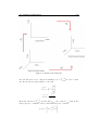
Wheel configuration
The configuration space of an omnidirectional mobile robot, is a smooth
3-manifold and can then be locally embedded in Euclidean space R3 . The
robot has three degrees of freedom, i.e., two dimension linear motion and
one dimension rotational motion. There are three universal wheels mounted
along the edge of the robot chassis 120◦ apart from each other, and each
wheel has a set of rollers aligned with its rim, as shown in Figure 3.8. Because of its special mechanism, the robot is able to simultaneously rotate
and translate. Therefore, the path planning can be significantly simplified
by directly defining the tracking task with the orientation and position errors obtained by the visual feedback.
For a nonholonomic robot, the robot’s velocity state is modeled as the
motion around its instantaneous center of rotation (ICR). As a 2D point in
the robot frame, the ICR position can be represented using two independent parameters. One can use either Cartesian or polar coordinates, but
singularities arise when the robot moves in a straight line (the ICR thus lies
at infinity). Hence, we used a hybrid approach that is defining the robot
40
Chapter 4. Control
position both in Cartesian and polar coordinates.
Normally, the position of the robot is represented by Cartesian coordinates which is a point in X-Y plane. By polar coordinates, the position
is described by an angle, and a distance to the origin. Instead of representing robot position with a single coordinate, the hybrid approach is used
as follows. The robot pose is defined as {XI , YI , α} where XI and YI are
linear positions of the robot in the world. Let α denote the angle between
the robot axis and the vector that connects the center of the robot and the
target object.
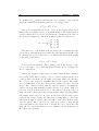
The transformation of the coordinates into polar coordinates with its
origin at goal position:
p
(4.1)
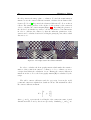
p = ∆x2 + ∆y 2 and α = −θ + atan2(∆x, ∆y)
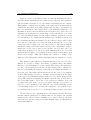
Then the calculated angle α is passed as the parameter to the simulator
in order to test the motor contributions calculated for the motion. Later,
the behavior tested with simulator is implemented for microcontroller with
Triskar function (in Appendix A.1), and the angle α calculated after acquiring the target, is passed to Triskar function, to calculate the motor
contributions on-board, to reach the target.
The inverse kinematics model is simple. It was considered that the representative coordinates of the robot were located in its center. Each wheel is
placed in such orientation that its axis of rotation points towards the center
of the robot and there is an angle of 120◦ between the wheels. The velocity
vector generated by each wheel is represented on Figure 4.1 by an arrow
and their direction relative to the Y coordinate (or robot front direction)
are 30◦ , 150◦ and 270◦ respectively.
For this type of configuration, the total platform displacement is achieved
by summing up all the three vectors contributions, given by:
−
→ −
→ −
→ −
→
FT = F1 + F2 + F3
First of all, some definitions need to be considered. Figure 4.1 represents
the diagram of the mobile robot platform with the three wheels. It was
assumed that the front of the robot is in positive Y direction, and the positive side to counter clockwise. The three wheels coupled to the motors are
mounted at angle position -60, +60 and +180 degrees, respectively. It is
4.1. Wheel configuration
41
Figure 4.1: The wheel position and robot orientation
important to remember that the wheel driving direction is perpendicular to
the motor axis (therefore 90 degrees more). The line of movement for each
wheel (when driven by the motor and ignoring sliding forces) is represented
in Figure 4.1 by solid, black arrows. The arrow indicates positive direction
contribution. The total platform displacement is the sum of three vector
components (one per motor) and is represented as a vector, applied to the
platform body center.
In order to find out the three independent motor contributions, the composition of the vectors represented by red arrows is projected on axes representing the line of movement of each wheel.
The calculation of the independent motor contributions is made using
the following formulas:


V t1


V t2  = MF ∗ V
V t3
42
Chapter 4. Control




−cosA sinA −1
VF




where MF =  cosA sinA −1 , V = 
VL

0
−1 −1
omega ∗ Rrobot
A is the angle of the front wheels, which is 30◦ for our robot. Indeed the
values (0.866, 0.5 ; -0.866, 0.5 ; 0, -1) in the Figure 4.1 coming from the
projection of cosine and sine of the motor vectors in the X-Y plane, which
are later used statically in the microcontroller for the calculation of the motor contributions. VF represents the frontal speed, VL lateral speed and
omega ∗ Rrobot represents the angular velocity of the body.
The vector of tangential wheel speed is represented as Vt1 ,Vt2 ,Vt3 and
vector of ”sliding” velocity of the wheels due to rollers is represented as
Vn1 ,Vn2 ,Vn3 . The vectors can have a positive or negative direction which
represents the direction in which the motor has to move (forward or backwards respectively). The desired speeds set as frontal speed (VF ) and lateral
speed (VL ) are projected through the motor axes in order to find motor contributions.
The angular velocity of the wheels is found by dividing the Vt of the
desired wheel to the radius of the wheel. It can be formulated as follows:
 

ω1
V t1
  

ω2  = V t2  /Rwheel
ω3
V t3

4.2
Matlab Script
In order to test the behavior we implemented a software simulator in Matlab,
that is calculating the motor contributions in order to go a specified position
in the world. It is possible to obtain three different movement model using
the inverse kinematics model. These are:
• Linear Movement
• Rotation
• Mixed Angular and Linear Movement
Linear Movement
4.2. Matlab Script
43
This is case where the angular speed of robot should be zero, and there
should be a linear movement in the displacement, which is the composition
of VF and VL vectors.
The software simulator that we built calculates the motor contribution.
The user inputs three variables (frontal speed, lateral speed and angular
speed) and the program outputs each motor contribution. Figure 4.2 shows
the result of the simulator for the linear movement forward.
vt1
vt2
200
vn2
v
n1
150
vF
100
50
0
−50
vF: 3500 mm/s
v : −350 mm/s
L
ωR: 0 rad/s
vt1: −3206.0889 mm/s
v : 1446.8911 mm/s
n1
vt2: 2856.0889 mm/s
vn2: 2053.1089 mm/s
vt3: 350 mm/s
vn3: −3500 mm/s
ω1: −130.3288 rad/s
ω2: 116.1012 rad/s
ω3: 14.2276 rad/s
vL
vn3
−100
−150
−200
−250
−300
vt3
−200
−100
0
100
200
300
Figure 4.2: A linear movement going slightly on the left on a line calculated by simulator
In Figure 4.2 VF represents the frontal speed is set to 3500 mm/s, VL
lateral speed to 350 mm/s and WR represents the angular velocity,which is
always 0 rad/s for the linear movement. The resulting motion is a linear
movement towards the direction which is the composition of VF and VL . The
motor contributions and their angular velocities are also shown in Figure 4.2.
44
Chapter 4. Control
Rotation
The second case is the rotation. For that particular configuration, we
only considered the movement caused by rotation without any displacement.
In the software simulator, the frontal speed and lateral speed are set to zero,
and the angular speed is calculated from the robot’s pose α using (4.1). An
example outcome of the simulator is shown in Figure 4.3. The robot is moving around its center with an angular speed of -0.099669 rad/s, without any
displacement in X-Y plane.
v
t2
200
150
100
ω
50
0
−50
v : 0 mm/s
F
vL: 0 mm/s
ωR: −0.099669 rad/s
v : 24.9172 mm/s
vt1
t1
vn1: 0 mm/s
v : 24.9172 mm/s
t2
vn2: 0 mm/s
vt3: 24.9172 mm/s
vn3: 0 mm/s
ω1: 1.0129 rad/s
ω : 1.0129 rad/s
2
ω3: 1.0129 rad/s
−100
−150
−200
vt3
−250
−200
−100
0
100
200
300
Figure 4.3: The angular movement calculated by simulator
All the theory for the calculation of the angular movement is same as
in the linear movement case, only values for some parameters change. The
angular velocity of the robot body ωR is calculated with α in the hybrid
approach we mentioned in the beginning of the section.
4.2. Matlab Script
45
Mixed Angular and Linear Movement
This is the case where the movement of the robot is composed of both the
angular and linear movement. In other words, the robot goes to the specified target while it is also rotating. The calculation made by the software
simulator uses all the parameters (frontal speed, lateral speed and angular
movement). The calculation of the frontal and lateral speed is found by subtracting the desired position of the robot from the initial position (Figure
4.4).
vt1
vt2
200
vn2
vn1
150
vF
100
ω
50
0
−50
v : 3500 mm/s
F
vL: −350 mm/s
ω : −0.099669 rad/s
v : −3181.1718 mm/s
t1
vn1: 1446.8911 mm/s
vt2: 2881.0061 mm/s
vn2: 2053.1089 mm/s
vt3: 374.9172 mm/s
vn3: −3500 mm/s
ω1: −129.3159 rad/s
ω : 117.1141 rad/s
2
ω3: 15.2405 rad/s
vL
R
v
−100
n3
−150
−200
−250
−300
v
−200
−100
t3
0
100
200
300
Figure 4.4: The mixed angular and linear movement calculated by simulator
In Figure 4.4, the resulting motion is not only a linear movement towards
the direction which is the composition of VF and VL , but also an angular
movement in clockwise direction with an angular speed of -0.099669 rad/s.
All these three different configurations are used in the implementation
of the robot. The whole script is found in Motion Simulator in Appendix
46
Chapter 4. Control
B.3. The most common used one is the mixed angular and linear movement.
Almost every path was initially implemented with this movement approach.
Others have been used where optimization is needed to cover problems due
to the lack of encoders to control the position of the motors.
4.3
PWM Control
Motors are controlled by applying a PWM signal to the H-Bridges. In order
to control velocity we did not use any encoders, so we don’t have feedback
about the motor rotation, or the displacement achieved with the result of the
applied PWM. To have an odometry information without using encoders,
we decided to review and replicate the work done at AIRLab about using
the mice odometry to get feedback from the motors. On the previously
work, a set of mice were reconfigured to obtain the position information,
and calculations were made from these readings to find the odometry. The
working configuration was able get a feedback when the distance between
the mouse sensors and lens was about 1mm, and the distance between lens
and ground was also 1 mm, but this distance is too small for our robot. In
order to increase the distance to 3 cm which is the distance between the
ground and the chassis of the robot, we experimented changing the lens of
the mice.
The mice work like a camera, and the image is captured by the sensor
inside it through a lens placed in front of it. We tested lenses with different
focal lengths and different orientations in order to achieve the 3 cm configuration. During the experiments, we obtained different performance on
different grounds and different lighting conditions. We tried several illumination alternatives, such as laser, led, and table lamp. We were able to find
the correct illumination using the led with a wave length readable from the
sensor. And for the lens we used a configuration with a focal length of 10
mm, leaving the distance between the lens and the sensor at 15 mm and
lens to ground at 30 mm. Instead of using encoders that each cost around
50 euro, the possible configuration costs around 5 euro, but the work is not
finished yet and we decided to include this on the robot later.
Since there is no information on the motor speed and displacement of
the robot, the control process mainly depends on vision, and it is not very
precise. There are situations where we cannot determine whether the motor
is moving. When the robot is stuck in a place and the sensors do not detect
4.3. PWM Control
47
a collision, such as entrance of the wheels to a gap in the floor, since we don’t
have a feedback on the motors we cannot determine whether the motors are
turning.
The motors are controlled by PWM generated from the microcontroller.
To drive motors we used a PWM signal and varied the duty cycle to act as
a throttle: 100% duty cycle = full speed, 0% duty cycle = coast, 50% duty
cycle = half speed, etc. After some testing we realized that the percentage
of the duty cycle and the speed are not changing with the same ratio (e.g.
50% of the duty cycle does not correspond the half speed). Also there is a
minimum percentage of the duty cycle which the wheels start turning, and
a maximum percentage of the duty cycle at which the speed remains as full
speed after that. The minimum PWM value to start the motion is % 45 of
the duty cycle and the speed set to full speed after exceeding the % 90 of the
duty cycle which is the maximum PWM that can be applied. Since there is
a non-linear increase between the ratio of rotation of the motors and applied
PWM rather than a linear one, the speed changes are not distinguishable.
In other words, the range of PWM signal that enables movement is very
narrow and the difference between the minimum speed and maximum speed
is not very apparent.
The script that is calculating the motor contributions according to the
target position is not taking into account the motor’s maximum or minimum speed. The script can return a motor contribution with 4000 mm/s or
3 mm/s which is cannot be performed physically by the motors. After some
experiments, to limit the script that calculates the motor contributions, we
decided to bound the PWM signal value to be applied to the motors. The
maximum PWM value defined for a motor is 2.5 meters/second and the
minimum PWM value is around 300 millimeters/second. Using both the
limits coming the physical characteristic of motor, and the PWM-rotation
limitations, we implemented a map that transforms the motor contribution
calculated by the script into a PWM signal. To do so, all the speeds between
2500 mm/s and 300 mm/s should be mapped to PWM signals between 45%
and 90% of duty cycle. Mapping 300 mm/s to the 45% and 2500 mm/s
to 90% did not resulted as expected since reflecting speed changes is not
possible.
In order to express most of the speeds, we decided to tune the PWM
sent to motors. Main idea is to bound to speeds in a dynamically changeable
manner. We introduced, a fuzzy-like behavior that is based on the robot’s
48
Chapter 4. Control
distance to the target position. Each distance is divided by a constant, then
multiplied with the multiplier defined as FAST, NORMAL and CLOSE.
Then another constant which is the minimum value that can initiate the
motors movement is added. Hence, the mapping that each value set by the
PWM signal generates a motion, is achieved. The multipliers are defined
according to the distance of the robot to the target object. For the distances
between 1200 mm and greater, the corresponding multiplier is classified as
FAST, between 1200 mm and 750 mm the multiplier is NORMAL, and for
the distances between 750 mm and 300 mm it is CLOSE. By defining such
control mechanism as FAST, NORMAL, CLOSE we are able to create three
different speed limits for the motors, which are all mapped from 60% to 85%
of the duty cycle where the motion is visible. As an example case, when
the robot detects a target at 3 meters, the motor speeds will be set with
multiplier FAST until the distance to the target reaches 1.2 meters. When
reached to 1.2 meters, the motor speed will be set with multiplier NORMAL
until the detected target distance is less than 700 millimeters. And finally,
the motors speeds will be set with multiplier CLOSE from 700 mm until the
target is reached. This mechanism allows to achieve more precision in the
motion, since the mapping guarantees that each motor speed set by PWM
will generate a reasonable motion. Moreover, instead of trying to map all the
speeds uniquely, indeed we are trying to map only one third of the speeds,
from the predefined speed ranges to 60%-85% of the PWM value in the duty
cycle. Even though the robot goes to target with an unexpected path, the
path is corrected as the robot comes closer since the slow motor speeds are
more precise and easy to achieve.
Even though the solution is not working perfectly, the robot is able to
go to the target successfully almost every time. The travel time and number
of movements in order to reach the target are not optimal, but this result
should be regarded as normal since we are not using any encoder to detect
the movement in the motors.
The need for an optimization of the PWM signal is also related to the
result of the miscalculation of the required torque. We selected motors that
do not have enough torque power for our robot. This brought the problem
of the arrangement of the PWM signal in order to run the motors. Since
the motors have less torque than we expected, almost 50% of the PWM is
wasted. First trials to optimize this inefficiency have been made by changing the frequency of the PWM to a higher or a lower frequency, but these
trials did not give good results. Later, we found the proper configuration,
4.3. PWM Control
49
mentioned previously, by limiting the minimum and maximum PWM values
of the motors and by introducing the fuzzy-like control to introduce different limits for the different distances to target. Even though the lack of the
encoders reduced the performance, we were able to produce an acceptable
configuration.
Another step is initialization of the motors. The corresponding pins in
the microcontroller for the motors are set to control the direction of motors
and PWM generation. The PWM generation is made by using the timers
available in the microcontroller. Output compare mode of the timers is
used in order to create the PWM needed to run the motors. Output compare
function is used to control the output waveform and indicates when a period
of time has elapsed. When a match is found between the output compare
register and the counter, the output compare function:
• Assigns a value to pins
• Sets a flag in the status register
• Generates an interrupt
Using the described output comparison, we created the desired PWM
wave to run the motors. At, first the timer clock is set to 8 mHZ. Then
output compare register 1 is set for the desired motor speed as some percentage of the full period of the cycle. Output compare register 2 is set
to full cycle that will set the pin to HIGH, and update the desired motor
speed of the output compare register 1. When counter reaches the defined
value, the motor speeds will be updated and the pins will be reset. It will
remain LOW until output compare register 2 value (which is the full period)
is reached. Using that algorithm we generate the PWM signal to run the
motor. For each motor, we decided to use a separate timer, since the timers
are available to use and not needed by other applications. It is also possible
to use only one timer to generate the PWM’s for all the motors using the
interrupts and output compare registers, but we decided not to use like this
for the simplicity of the algorithm, since this will need a better synchronization, and optimization to run efficiently.
The control of the servo that is changing the camera head pointing direction is also implemented using PWM signals. For the servo PWM, we don’t
have the problem of control that we faced with the motors. So, no tunings
50
Chapter 4. Control
are implemented for this case, and the PWM creation is implemented simply as follows. The PWM which controls the servo position is implemented
with the first timer at with the motor. The period of PWM in first timer,
to control the motor, is divided by a constant in order to achieve a smaller
PWM period, which is around 2ms for the servo. The rest of the idea is the
same. The PWM is generated with the help of the output compare mode.
The servo position is initialized at the same time with the motors, then
the position is controlled calling the Position Camera(); function that can
take SERVO TOP, SERVO MID, SERVO BOTTOM as the different positions for the camera servo. Indeed this camera positions are used during the
vision inspection to reach the target and calculate the motor contribution
according the distance of the target object. 3 unique camera head position
are implemented using the visual feedback from the ST software, to find the
best configuration in terms of depth of field and field of view. If the target
is more far than 750 mm the camera position is set to SERVO TOP, which
can see the environment from 750 mm to robot up to 4-5 meters. If the
target is closer than 750 mm to robot, the camera head position is lowered
to SERVO MID, in order to provide a vision from robot boundary to 750
mm. The last position is implemented for testing reasons, and also provides
a ready configuration to set the camera head in any position.
Chapter 5
Vision
The vision system is focused on the implementation of the camera for object
detection and calculating the position of this object according to the robot.
To do so, the relation between different coordinate systems, which are image
plane coordinate system, robot coordinate system, and real world coordinate
system, should be defined. In order to go to the target, it is necessary to
know where the object is placed. Using the blob search algorithm, we acquire the position of the object in the pixel coordinates. We need a mapping
between those three coordinates to command the movement. There are several approaches to determine the object position according to the robot, as
mentioned in Chapter 2. Among those, we will use the one for the calibrated
cameras.
The rest of Chapter describes camera calibration, the script that calculates the transformation, color definition, and the script to define the color.
5.1
Camera Calibration
The initial step for the algorithm is to find the camera calibration. The
Camera Calibration Toolbox [2] is used to calculate the camera calibration
matrix that is necessary to find the projection between the world and image
points represented by homogeneous vectors. Normally, the object is placed
on the real world coordinate systems, and its position can be measured from
the origin. In order to find the distance of the camera plane to the object,
we need a transformation that maps the 3D points (for the object that is
assumed to place in ground, the point is a 2D point in world coordinates,
since height is 0 all the times) of the objects in the 3D world coordinates to
52
Chapter 5. Vision
the 2D points in the image plane coordinates. To find the transformation
matrix, we use the camera calibration matrix, calculated from Camera Calibration Toolbox [2]. In general, the Camera Calibration Toolbox works as
follows. The sample pictures of the checker board it taken by the camera in
order to calculate the camera matrix (Figure 5.1). By taking the pictures of
the checker board makes it possible to use the information of its dimensions
in order to calibrate the camera, by that the unknown parameters of the
camera can be calculated such as focal length, principal point, skew, radial
distortion, etc.
Figure 5.1: The images used in the camera calibration
In order to calculate the homography matrix, which makes the transformation of the points from camera coordinate to robot coordinate, we wrote
a script that makes the calculation for us. Having the camera calibration
matrix from the toolbox, the homography matrix (H) is calculated by the
script.
The whole camera calibration and the projection between the world
points and camera as explained in details as follows. The matrix K is called
the camera calibration matrix.


K=
fx
fy

px

py 
1
where fx and fy represent the focal length of the camera in terms of pixel
dimensions in the x and y direction respectively. Similarly, px and py are
5.1. Camera Calibration
53
the principal points in terms of pixel dimension.
x = K[I|0]X cam
where Xcam as (X, Y, Z, 1)t to emphasize that the camera is assumed to be
located at the origin of a Euclidean coordinate system with the principal
axis of the camera point straight down the z-axis, and the point Xcam is
expressed in the camera coordinate system.
In general, points in the space will be expressed in terms of a different
Euclidean coordinate frame, known as the world coordinate frame. The two
frames are related via a rotation and a translation. The relation between
the two frames can be represented as follows:
x = KR[I| − C]X
where X is now in a world coordinate frame. This is the general mapping given by a pinhole camera (In Figure 5.2). A general pinhole camera,
P = KR[I| − C], has a 9 degrees of freedom: 3 for K, 3 for R, 3 for C.
The parameters contained in K are called internal camera parameters. The
parameters of R and C which relate the camera orientation and position to
a world coordinate system are called the external parameters. In a compact
form, the camera matrix is
P = K[R|t]
where t = −RC.
The camera matrix, which consists of internal and external camera parameters, is calculated by the camera calibration toolbox automatically.
Having the internal and external camera parameters from the toolbox, we
compute the homography H. Homography is an invertible transformation
from the real projective plane to the projective plane.
We developed two different approaches to determine the position of a
target according to the robot coordinates. In the first case, the target object is a ball, and we are using the information coming from the diameter
of the ball. In this case, the transformation should be a 3D to 2D, since the
ball can be represented in world coordinates system with the X,Y,Z and in
the camera coordinates with two values X,Y. In the second case, we assume
that the target object is on the ground and we are using the information
coming from the intersection point of the object with the ground. This
54
Chapter 5. Vision
Figure 5.2: Perspective projection in a pinhole camera
means the object can be represented by a X,Y,Z position in the world coordinate system, with Z=0. This reduces the transformation into a 2D-2D
transformation, and needs a new H matrix.
We need to calculate the transformation matrix between the robot and
camera (TCR ) coordinates. The transformation matrix between world frame
C ) coordinates is known from the external camera parameters.
and camera (TW
R is calculated by
The world frame to robot frame transformation matrix TW
the target object position and robot center (shown in Figure 5.3). TCR is
derived as follows:
R
TCR = TW
∗ TCW
For the ball localization case, the calculation is made for the pixel diameter D px of the ball at known distance l and the real diameter D ball . For the
camera, we introduced a parameter f ∗ , to indicate the dimension of a unit
pixel, which is a statical parameter of the camera. Using this information,
the distance of the ball lnew can be calculated by counting the pixels of the
diameter of the ball D px and by multiplying this by f ∗ .
f∗ =
lnew =
l
D ball
∗ D px
f∗
∗ D ball
D px
−−−→
The next step is converting the direction from camera to the ball dc ball
5.1. Camera Calibration
55
Figure 5.3: Camera robot world space
−−−−→
into the direction vector, and its normalized vector dc norm in order to find
the direction from camera plane to the ball.
 
u
−−
−→
 
dc ball = K -1 ∗ v 
1
−−
−→
−−
→
dc ball
c−−
d norm = −−−→
|dc ball |
−−−−→
From the direction dc norm and the line lnew , the point P c ball that is 3D
homogeneous coordinates of the points with respect to camera.
"
−−
→#
c−−
l
∗
d
norm
P c ball = new
1
56
Chapter 5. Vision
To calculate P R ball which is 3D homogeneous coordinates of the point in
world, the transformation matrix camera to robot (TCR ) is used.
P R ball = TCR ∗ P C ball
The second configuration is for the object on the ground. This case is
simpler since it requires a 2 D to 2 D transformation. The transformation
between camera and robot is used again and the calculation is the same as
the previous configuration. The homography is defined for this case as:


1 0 0
0 1 0


H = K ∗ TRC ∗ 

0 0 0
0 0 0
The third row of the matrix is all zeros since the we assume that the
object is at ground with Z=0, hence this reduces the mapping from 3D to 2D.
To calculate the object position Pobject , we will use the inverse homography
on the image point Pimage .
P object = H -1 ∗ P image .
Pobject is then normalized. The resulting point is the distance of the
robot to the target object. This information is later used to calculate the
motor contributions.
Among the mentioned approaches, we started with the first configuration (for the ball). The idea was to detect a ball, no matter whether it is
on the ground or up in the air. We started by testing with a red ball, since
the color red, blue, green were initially defined for the camera. The results
were not sufficient to follow the ball for greater distances because of several
effects. One of them is related with the camera resolution. Normally the
camera can work with 160x120 resolution for the blob search. This does
not cause a problem if the ball is close to the camera, but as the ball goes
further from the camera, the ball represented in the image is getting smaller
and smaller. Due to the low-cost optics, at the worst case the ball becomes
1 pixel in the picture. Using only this pixel, it is impossible to detect the
ball. Even though, we can recognize the ball for some cases, in most of the
cases we cannot. Due to the low-cost optics, it is possible to have several
other 1 pixel size red blobs that are not our ball. In order to detect the ball,
inside the blob search algorithm we need to eliminate the blobs that are not
the ball we are searching.
5.1. Camera Calibration
57
Later, in order to solve this problem, we came up increasing the size of
the ball. Again, this trial did not resulted as we expected, since when the
ball gets further from the robot, the diameter information is not reliable.
This results to calculate a wrong value of the ball position. In this trials, we
realized also the effects of the white balance and exposure compensation for
the color information. The camera tries to automatically adjust the color
information as the ball gets further from the light source. Since the blob
elimination is dependent on both the shape of the ball and the color of the
blob, the information changed by the camera results to definition of wrong
blob information. To clarify with an example, the ball shape is checked by
the circularity information calculated by the camera, but the whole ball is
not composed of the same color, since the light is affecting the color, so the
center can be more bright or the corner more dark etc. The camera with the
automatic setting of the white balance and exposure compensation tends to
change the color in order to have a better picture, but by doing so the color
temperature is changed. So the blob search eliminates the non-color points
as well as the non-shape objects and detects the ball in another shape, such
as an open rectangle. This whole change also results to a change of the
diameter of the ball and the distance information is not calculated correctly.
The diameter of the ball is a problematic issue due to the low-cost optics.
Instead, we decided to change our ball into a cylindric shape and assume
that the object will always be on the ground. This reduces the mapping to
a 2 D to 2 D mapping problem, since Z (the height) will be always zero.
Instead of calculating the diameter of the ball, we determine the distance between the end of the image and the intersection point of the object with the
ground. This distance is easier to measure, independently from the shape
of the object, and will always change as the object’s position changes in the
world. The mentioned mapping also makes easier the blob search, since it
is not very important to detect the object clearly as a cylindric. If we can
recognize some part of the object we can ensure that the object is more or
less close to the calculated point. This also gave us the flexibility for the
color information, since we do not have the obligation to detect all the object,
we can define a more generic color code that is working for most of the cases.
We used the second configuration in both camera positions. Even the
internal camera parameters are always same in our camera, the external
parameters are effected with a translation or rotation. Indeed, when the
camera head position is changed, it results with the usage of a H matrix for
each transformation.
58
Chapter 5. Vision
The whole algorithm and script is found in Object’s Position section in
Appendix B.2
5.2
Color Definition
The camera we are currently using has a UXGA resolution CMOS and it is
set to 160x120 resolution for the blob search algorithm. One major problem
is the blob search algorithm. The algorithm used inside is unknown and
this forced us to define color information very precisely, since we cannot
eliminate the non-object blobs easily. We can eliminate the problem only
by using the area, perimeter and the circularity information which, in case
the target is a ball, is not enough for most cases to track the blob. So this
makes the color definition important. The color is defined in a RGB Cube,
using RGB444 format, and it is not very clear to understand the correctness
of the defined color from the color codes. In order to ease this process, the
color selection is made by the ST software by selecting the desired color from
the image, or directly programming the rules if the color values are known.
Since the resolution is very low, the color consists of shadows, or existence
of blob not belonging to the searched object made us to improve the color
selection. The current ST software is sufficient to visualize the selected color
and test the blob search, but color definition is difficult since, in order to
define the color, the pixels should be selected one by one, is not possible
to select an area. Moreover, the rules (which is the additions and subtractions of the color codes to RGB Cube) found by the ST software are not
in the compact form (the same rule for a color can be added or subtracted
more than one). To improve the color selection, we decided to use an offline calculator, that calculates the histogram for the selected object’s colors.
As a first step, we started by disabling automatic white balance and automatic exposure control. Before getting into the white balance, the concept
of color temperature needs to be introduced. Color temperature is just a
way of quantifying the color of light. It is measured in degrees Kelvin (K).
Normal daylight has a color temperature of around 6,500K. Warmer light
has a lower color temperature. The warm light that occurs late in the afternoon might have a color temperature of around 4,000K. Cooler light has a
higher color temperature. The bluish light that sometimes occurs in twilight
periods of the day might have a color temperature of about 7,500K. So, our
concept of warm and cool light is tied directly to the color temperature. The
5.2. Color Definition
59
warmer (yellow) the light, the lower the color temperature; the cooler the
light (blue), the higher the color temperature.
Color Temperature
1000-2000 K
2500-3500 K
3000-4000 K
4000-5000 K
5000-5500 K
5000-6500 K
6500-8000 K
9000-10000 K
Light Source
Candle light
Tungsten Bulb (household variety)
Sunrise/Sunset (clear sky)
Fluorescent Lamps
Electronic Flash
Daylight with Clear Sky (sun overhead)
Moderately Overcast Sky
Shade or Heavily Overcast Sky
Color temperature is also important for cameras. The camera manufacturers knew that the color of the light would affect the colors delivered by
the camera. Therefore, they decided to deal with the problem by designing
the cameras to automatically measure the light temperature and to make
adjustments as the light changes color. That is why we can shoot in the relatively neutral light with camera in the afternoon and then shoot the next
day in the cool light of early morning and still, probably, get reasonable
colors in both situations even though the color of the light was different.
Cameras correct for the change in light temperature, using white balance.
With auto white balance, the camera attempts to determine the color
temperature of the light, and automatically adjusts for that color temperature. Auto white balance works reasonably well under the following conditions:
• The application does not require absolute maximum color accuracy
• There is not a preponderance of one color in the scene being photographed
• Adjustments for the color temperature of the light
As mentioned in the previous paragraph, in auto white balance mode, the
camera does its best to determine the color of the light and make appropriate
adjustments. However, the methodology that is used to do this requires
that certain assumptions be made. These assumptions do not always match
perfectly the scene being photographed. As a consequence, the auto white
balance option does not always yield perfect results. Accordingly, problems
60
Chapter 5. Vision
may occur using auto white balance when the conditions listed above are
violated. Therefore, auto white balance may not be a good choice if:
• Absolute color accuracy is required
• There is a lot of one color in the scene: The preponderance of one
color can fool the auto white balance function into assuming that the
light has a lot of that color in it. This can result in an incorrect white
balance and a color cast.
• No adjustments made for the temperature of the light wanted: In
certain cases, the color of the light is what makes the photograph. A
sunset is an example. Without the rich, warm colors of the light, a
sunset just isn’t a sunset. Auto white balance may attempt to make
adjustments to correct for the warm color of the sunset light. This
would produce an image with less saturated colors or colors that were
different than what has been seen.
The camera we are using supports different settings for the balance. These
are:
• OFF - No White balance, all gains will be unity in this mode
• AUTOMATIC - Automatic mode, relative step is computed here
• MANUAL RGB - User manual mode, gains are applied manually
• DAYLIGHT PRESET - DAYLIGHT and all the modes below, fixed
value of gains are applied here.
• TUNGSTEN PRESET
• FLUORESCENT PRESET
• HORIZON PRESET
• MANUAL color TEMP
• FLASHGUN PRESET
Among the possible options, we set the white balance OFF. Because, in
the application we require absolute color accuracy and we don’t want the
camera to change the temperature of the color since we want to detect the
target with a constant color parameter defined using the samples we took.
5.2. Color Definition
61
Another automatic adjustment can be done on exposure. Subjects lighter
than middle gray, such as a white china plate, reflect more than 18% of the
light falling on them. The exposure system doesn’t know that the scene
should look bright, so it calculates an exposure that produces a middle gray
image that is too dark. Subjects that are darker than middle gray such as
black cloth, reflect less than 18% of the light falling on them. The exposure
system calculates an exposure that makes the image middle gray and too
light.
The contrast or difference in brightness between the subject and the
background can fool an exposure system, particularly if the subject occupies a relatively small part of the scene compared to the background. The
brightness of the background is so predominant that the automatic exposure
system adjusts the exposure to render the overall brightness as a middle gray.
If the main subject is lighter than the background, it will be overexposed
and too light. If it’s darker than the background, it will be underexposed
and too dark.
Depending on the arrangement of the lighting, some subjects may be
too contrasty with brightly lit highlights and deep shadows. The range of
brightness may exceed the range that can be captured by the camera. In
these cases adjustments should be made in the lights to balance out the
light and to lower the contrast. However, deciding whether the highlight or
shadow areas are most important for the final picture, the exposure setting
should be made appropriately.
The perfect exposure retains details in both the highlights and shadows.
For the auto exposure system, this is as difficult. If there is even a little too
much exposure, the image is too light and details are lost in the highlights.
If there is too little exposure, the image is too dark and details are lost in
the shadows.
When confronted with any subject lighter or darker than middle gray,
exposure compensation is used to lighten or darken the photograph that the
camera would otherwise produce.
To lighten a picture, the exposure is increased. This is useful for setups
where the background is much lighter than the subject, or when photographing very light objects, such as white china on a white tablecloth. To darken
an image, the exposure is decreased. This is useful for setups where the
62
Chapter 5. Vision
background is much darker than the subject, or when photographing very
dark objects, such as black china on a black tablecloth.
From the parameters available in our camera we disabled the automatic
exposure by setting DIRECT MANUAL MODE, in which the exposure parameters are input directly and not calculated by the camera. We don’t
want the camera automatically adjust the exposure, since this will cause to
lighten or darken the picture dynamically. Instead by setting the exposure
directly to a constant value, we ensure that the picture will remain with the
same enlightenment, together with the target we are searching for.
After setting the white balance and exposure compensation, we took
sample images (Figure 5.4) in order to define selected object’s color using
the script.
Figure 5.4: Samples are taken from different lighting conditions and different distance
to the target object
After acquiring the samples, the next step is creation of the histogram,
to find the distribution of the RGB values in the target object’s color. The
histogram created is shown in Figure 5.5.
An image histogram is a type of histogram that acts as a graphical representation of the color distribution in a digital image. It plots the number of
pixels for each color value. By looking at the histogram for a specific image,
5.2. Color Definition
63
R
G
9000
B
6000
7000
8000
6000
5000
7000
5000
6000
4000
4000
5000
3000
4000
3000
3000
2000
2000
2000
1000
1000
1000
0
0
2
4
6
8
10
0
0
2
4
6
8
10
12
0
0
2
4
6
8
10
Figure 5.5: The histogram formed from the samples taken for each color channel.
a viewer will be able to judge the entire color distribution at a glance. For
this we wrote a script in Matlab. We took as many samples as we could from
the environment where the object is placed in different lighting conditions.
From the sample images captured, the part with the object is cropped
(area with the target color) in order to find the color distribution of the
pixels forming the object.
(a) Mask R
(b) Mask G
(c) Mask B
Figure 5.6: The mask for each channel by setting the upper and lower bounds.
From that histograms we create the masks (Figure 5.6), by finding the
upper bounds and lower bounds for each color channel. As a final step we
create the total mask, that is returning the target object’s color boundaries
64
Chapter 5. Vision
in a form that can be converted into the rules. The result of the color selection script, with the original picture is shown in Figure 5.7.
(a) Mask to be Applied
(b) Orginal Picture
Figure 5.7: The mask applied to the orginal picture.
The boundaries found for the object are converted into rules, that will
add or subtract the color from the RGB Cube. The rules are checked by
color selection program, provided with the ST software coming with the
camera. The script can be found in Appendix B.1 in Color Histogram Calculator. Using both the color selecting program and an offline Matlab script,
we have been able to define the color in a more precise way, and improved
the results for object detection. But the results diverged as the lighting
conditions change in the environment. For example the laboratory where
we have performed tests is exposed to direct sunlight in the morning, while
in the afternoon it is not. We introduced different configurations for the
same color, to avoid the need for sampling of the previously defined color.
By controlling the color before each run manually and recalculating when
necessary resulted a stable solution to the problem.
5.3
Tracking
The final working configuration of the object detection is made by solving
the problems described previously. We can explain these in three titles.
First one is finding the correct color information. We start by disabling the
automatic white balance and automatic exposure compensation. This allows
us to have the color as it is seen directly from the camera, by not adjusting
5.3. Tracking
65
any color values. It means, if the object is exposed to light, the parts that
are exposed to light are not considered as white but a tone of target color,
similarly with the previous configuration the dark pixel such as the parts in
the shadow are considered as black, but with the new configuration they are
also considered as a tone of the target color.
Second step is calculation of the color information in a better way. Previously, we calculated the information by ST color picker software. With
this software we select the color region we want to assume as the blob color.
The problem of this approach is that the blob may not consists of a single
rule (RGB color code). Some parts of the object are darker, some parts
are lighter. Also with the distance, the color that is composing the object
is changing. Additionally, the colors that are not considered as red, blue,
green, represented again as rules (RGB color codes) and it is not possible to
understand by just looking at the color code whether it is the correct color
coding or not. These makes it very difficult to determine the color with the
ST color picker software. Instead, we decided to find the color histogram
that is the distribution of the selected color properly in the RGB channels
separately. To do so, we took several samples from the camera, in different
distances, in different illuminations to find a proper average. The calculated
results are later tested with the ST color picker software, since it offers a
good interface to see whether the color is selected correct or not, in a visual
way.
The third step is related to the estimation of the objects distance to the
robot. As mentioned before, the diameter of the ball is a problematic issue
due to the low-cost optics, hence we decided to use an object with cylindric
shape, and the second configuration for the transformation. This distance
is easier to measure, independently from the shape of the object, and will
always change as the object’s position changes in the world.
During the implementation to the microcontroller to increase the performance, we tried to avoid matrix and floating point operations. The matrices
that can be defined statically are defined statically. To avoid floating point
operations, the floating points are converted into integer, then multiplied by
a constant (most of the times 1000). The operations are made in integer,
and the result is returned as floating point by dividing with the constant.
We ensure that the microcontroller will not spend too much time in matrix
and floating point operations, using this approach.
66
Chapter 5. Vision
Chapter 6
Game
The robot will be used as a testbed to develop robogames. As a testbed a
simple game is implemented, using almost all the components available on
the robot. The game is used also to verify the correctness of the solutions
implemented. We created a simple game to test the robot. Basically, the
robot has to go to several targets in a sequence, by avoiding obstacles, until
the final target is acquired.
The game flow can be expressed in a better way with an algorithmic
approach. The class diagram is shown in Appendix A.1 and the flow diagram in Appendix A.2. The microcontroller starts by controlling the game
end status. The game end status is composed of conditions. First, it checks
whether the target is acquired. If it is acquired then it also checks whether
this is the last target and ends the game by staying at the current position.
If it is not the last target, the algorithm steps from the game status check
phase and continues the search. Before performing any other operation the
collision status is controlled. If a collision is detected, a proper command is
sent to motors to get rid of the obstacle.
The next step is blob search, and blob tracing. The camera searches for
the target at its vision side. If no blob is found, the robot performs a turn
around its center of rotation until a blob is found or a collision detected.
Normally, the collision should not be controlled for the turn around the
center of rotation but, as we discussed previously, we cannot guarantee the
correctness of the movement since we lack encoders for the motors. When a
blob is found, the first step is checking the color information of blob, since
the difference between targets is made by the color information. If the cor-
68
Chapter 6. Game
rect target is found, we calculate the distance of the object from the robot.
According to the distance found, the motor contributions are calculated and
the robot starts going to the target.
We introduced two different camera head positions. At the start the
camera is always set at the normal position (which can see the environment
from 750 mm from the robot up to 4-5 meters). According to the result
of the distance calculated at the previous step, the camera head position
maybe be lowered in order to detect and go to the target in the next step.
The target is set as acquired when the distance between the robot and the
target is below a certain threshold. The whole algorithm we can be seen in
Appendix A A.2 in a clear way.
The software that is running the robot is working on-board, on the microcontroller. The software is divided into sub-modules in order to ease
the development of the process. In this section, we will give the details of
the software, introducing the sub-modules, supporting with the diagrams.
The software is composed of low-level and high-level modules. The lowlevel modules are the assembly code that is coming with the ST tool-chain,
which already defines the registers, memory mappings, all the communications with the chips. We did not concentrate on the assembly code; all the
written software implements the high level part.
The development mainly focused on the generation of PWM using timers,
initialization of components, algorithms and utilities. Like all the microcontroller programs the core runs in the main loop. Before entering the main
loop we initialize all the components first. Initialization is made step by
step as follows:
• Configure the system clocks
• Configure the GPIO ports
• Configure x24 Camera
• Configure the USB
• Initialize camera parameters
• Initialize motors
• Set initial camera position
69
• Initialize sensors
• Initialize the blob search and color parameters
In order to initialize the camera, the RGB Cube which contains the color
information and BlobSearch are initialized. We also set the automatic white
balance to off and exposure control to direct manual mode. The appropriate
parameters for the image format, frame rate, sensor mode and clock are set
for the blob search at this point.
The second step is initialization of the motors. The corresponding pins in
the microcontroller for the motors are set to control the direction of motors
and PWM generation. The PWM generation is made by using the timers
were available in the microcontroller. Output compare mode of the timers
used in order to create the PWM needed to run the motors. Output compare
function is used to control the output waveform and indicate when a period
of time has elapsed. When a match is found between the output compare
register and the counter, the output compare function:
• Assigns a value to pins
• Sets a flag in the status register
• Generates an interrupt
Using the described output comparison, we created the desired PWM
wave to run the motors and camera servo.
The sensors, which are the bumpers for the current state of the robot,
are initialized by setting the corresponding pins in the microcontroller.
As a final step in the initialization, the blob search and color parameters are set. The blob search parameters, which are grid size, top, bottom,
left and right borders of the image are defined. Similarly the blob search
geometry options are defined, which are the color id, minimum-maximum
area of the blob, minimum-maximum circularity of the blob and minimummaximum perimeter of the blob. For each color, the blob search geometry
options should be defined separately with the proper coding.
Lastly, the color information should be defined for each color we are
searching. The color information is calculated either by the ST color picker
70
Chapter 6. Game
software or from the Matlab script taking samples from the environment in
order to calculate the histogram to find the correct color coding. The color
values found from the Matlab script should be tested with the ST color
picker software in order to check the correctness of the results.
After the initialization phase completed, the main control loop starts.
Before entering the main control loop, the parameters, such as search direction,
game end, color done, blob found etc., that are going to be used locally inside the main loop are set to initial values. The main loop starts by reading
the values of the sensor data. Later, the ’color done’ status, which is controlling the target acquired condition. Initially, it is set as ’FALSE’, since
the camera did not acquire any images. Before capturing any image, the
’control hit’ is checked to detect and clear the hit. Until no collision is
detected, the capturing of the images will not start. After the capturing is
complete, the blobs found with the correct color, if any, are sorted according
to the their area, and the one with the maximum area is set as ’myBlob’.
If no blob found in this step, ’myBlob’ is set to -1 to indicate no blob is
found within constraints. The sign of the ’myBlob’ is controlled to check
whether a blob is found or not. If no blob is found, ’blob found’ or ’counter’
status is checked. This part is implemented so that to decrease the number
of turns, for each time a blob is not found. Having the ’counter’ less then
3, we increment the counter, and do not perform any turns. In the case
the ’counter’ is greater than 3 or ’blob found=FALSE’, we perform a turn
around the center, and set the ’blob found=FALSE’. That mechanism enabled us to detect a target, that was not detected even if it is on side. Even
if the target is on side and it is not detected for 3 times, we perform the
turn. To process blob, in ’myBlob’ parameter, the first step is controlling
the camera position. Depending to the camera position, the position of the
target in real world is calculated. The motor contributions are calculated
using ’Triskar’ function. According to the calculated position of the target
the following cases is executed. If the camera is set to SERVO TOP and the
distance of the robot to the target is:
• Greater than 1200 mm.
The motor speeds from Triskar are set with multiplier FAST
• Between 1200 mm and 700 mm.
The motor speeds from Triskar are set with multiplier NORMAL
• Less than 700 mm.
The camera head position is changed to SERVO MID
71
If the camera is set to SERVO MID, the position of the target is calculated with ’CalculatePositionGround’ function. The motor contributions
are calculated using ’Triskar’ function, and the motor speeds from ’Triskar’
are set with multiplier CLOSE. If the distance of the robot to target is less
than 300 mm, the target is marked as acquired by setting ’color done =
TRUE’.
The detection of target acquired and game-over is done by controlling
’color done’ on every loop. When the ’color done’ is set as ’TRUE’, the
camera head position is set to SERVO TOP, ’color done’ and ’blob found’
are flagged as ’FALSE’, and color is incremented by 1. Since the current
configuration is working with 2 colors, the case where ’color > 2’ is controlled for the game-over case. For that case, we introduced a variable as
’reply counter’, which sets the number of replies/rounds to end the game.
In the code, this variable is set as 5, that made the game to find and go to
the targets 5 times, in the same color order defined. The work flow in the
main loop is shown in Appendix A.2.
The class diagram that is showing the relation between the modules
is reported in Appendix A A.1. We increased the modularity of the program by separating the code to improve reuse; breaking a large system into
modules, makes the system easier to understand. By understanding the behaviors contained within a module, and the dependencies that exist between
modules, it’s easier to identify and assess the ramification of change. We
used the naming convention Init for initialization classes, functions. The
algorithm are implemented inside the Motion and Vision classes. The motion algorithm is implemented by porting the software simulator previously
written to the microcontroller. The vision algorithms are also implemented
in a similar manner. The camera calibration calculating the position of the
object was previously implemented in a Matlab script. Later, the script has
been ported to the microcontroller.
The rest of the implementation not mentioned above, focuses on pin
assignments (in Appendix D.3), definitions of the constants, creation of the
header files.
72
Chapter 6. Game
Chapter 7
Conclusions and Future
Work
After the tests performed, proper modifications have been implemented to
solve the detected problems discussed previously. At last, we have been able
to obtain a working robot, satisfying most of the constraints defined at the
beginning. The robot dimensions are more or less same with the designed
dimensions. Even though, we don’t have a proper method to measure the
robot’s maximum speed, the maximum speed achieved by the robot is fast
enough as expected. The obstacle avoiding is implemented with bumpers,
and supported with foams and springs. The camera head is placed on a
servo, can be moved up and down. The fully charged batteries provide
enough power to move the robot for at least 2 hours. It is difficult to estimate the total price of the robot. The camera board that is used, is not
available in the market, and the total cost of the components in camera board
might be misleading to determine the cost of the camera board. Moreover,
for the other components, the prices show differences as the order quantity
changes. In conclusion, the final price might match the cost constraint 250
euro.
The robot is fully working autonomously, playing the designed game
without any interruption. The game is finding the predefined colored objects and going to them in the defined order. We tested the game with
two objects colored in orange and green. More colors and objects can be
introduced easily following the steps indicated in Appendix C. The color
detection must be made with the color calculator script and must be tested
with the ST color picker software. In order to have stable performance, it
74
Chapter 7. Conclusions and Future Work
is advised to check the colors before each run, since the illumination of the
environment can change the color interpretation. We defined two different
configurations for each color, one for the sunny day, the other for the cloudy
day, both are working at our testing environment.
In order to solve the problems related to vision, color selection script,
a custom white balance and an auto exposure is used to improve the behavior of the system affected by low cost vision. The problems arisen from
the motor control is solved by limiting the minimum and maximum PWM
values of the motors and by introducing the fuzzy-like control to introduce
different limits for the different distances to target. The use of these tunings and optimizations enabled us to select low cost components, which are
performing enough well to develop a robot framework that will be used as
a basis to implementing different robogames.
As for the future developments, we plan two additions. The first one it
is the development of a dock station and implementation of the autonomous
charging behavior. The circuit to measure the battery level is already operational. The software to check the battery level and then go to the dock
station must be implemented.
The second addition is the mice boards that we are going to use as
odometers. Experiments have been made to modify the previous work done
at AIRLab, using the mice as an odometry device. We have not been able
to design the working prototype, and the control circuit that calculates the
position information from the mice yet. Previously, the position information was calculated with a PIC and a PC. The new design will work on the
ARM microprocessor, and the interface between the camera board and mice
should be designed and implemented.
The third addition is the self adaptation of the robot to battery charge
level. Using the output of battery monitoring circuit, the battery level can
be measured. These measurements are going to used in the implementation
to detect the battery level and change the speed multipliers to keep the
robot in the same speed, even if the battery level is going low. Also, the
robot is going to adapt itself to make the decision of going to the docking
station for reaching, when a low battery status detected.
Implementation of the future developments will result to have a better
control in motion mechanism and introduce more autonomous robot behav-
75
ior, which will be useful in the research line to develop more interesting
robogames.
76
Chapter 7. Conclusions and Future Work
Bibliography
[1] Battle bots-http://www.battlebots.com/.
[2] Camera
calibration
toolbox
for
matlab
http://www.vision.caltech.edu/bouguetj/calib doc/index.html.
-
[3] First robotics competition-www.usfirst.org/uploadedfiles/who/impact/brandeis st
udies/05fll underserved summary.pdf.
[4] Item-http://www.item24.com/en.
[5] Lego group - http://mindstorms.lego.com/en-us/default.aspx.
[6] Lifelong kindergarten-http://llk.media.mit.edu/projects.php.
[7] Logo foundation-http://el.media.mit.edu/logo-foundation/.
[8] The mars autonomy project-http://www.frc.ri.cmu.edu/projects/mars/.
[9] Microsoft
actimates
interactive
barney
to
teract
with
”barney
&
friends”
on
http://www.microsoft.com/presspass/press/1997/sept97/
spr.mspx.
inpbsmspb-
[10] Plexiglass physical properties - http://www.rplastics.com/phprofplac.html.
[11] Robowars-http://www.robowars.org.
[12] Working
with
aluminum
http://www.searchautoparts.com/searchautoparts/article/articledetail.jsp?id=162604.
R
[13] Intel
playTM me2cam
computer
video
http://www.intel.com/support/intelplay/me2cam/.
ration, 2008.
camera
Intel Corpo-
R
R
[14] irobotroomba
vacuum
cleaning robots. iRobot Corp, 2008.
77
78
BIBLIOGRAPHY
[15] A. Eliazar and R. Parr. Learning probabilistic motion models for mobile
robots. In Proceedings of the twenty-first international conference on
Machine learning, 2004.
[16] N. Tomatis A. Tapus and R. Siegwart A. Martinelli. Simultaneous
localization and odometry calibration for mobile robot. IEEE/RSJ
International Conference on Intelligent Robots and Systems, 2003.
[17] M. Asada, R. D’Andrea, A. Birk, H. Kitano, and Manuela Veloso.
Robotics in edutainment. In Proceedings of the IEEE International
Conference on Robotics and Automation 2000 (ICRA ’00), volume 1,
pages 795 – 800, April 2000.
[18] Bobick et al. The kidsroom. Communications of the ACM, Vol. 43,
No. 3, 60-61, 2000.
[19] A Bonarini. Designing highly interactive, competitive robogames. AIRLab report, 2010.
[20] David Cavallo, Arnan Sipitakiat, Anindita Basu, Shaundra Bryant,
Larissa Welti-santos, John Maloney, Siyu Chen, Erik Asmussen, Cynthia Solomon, and Edith Ackermann. C and ackermann e: âroballet:
exploring learning through expression in the arts through constructing in a technologically immersive environment. In in Proceedings of
International Conference on the Learning Sciences 2004, 2004.
[21] M Tan and Y Shen D Xu. A new simple visual control method based on
cross ratio invariance. IEEE International Conference on Mechatronics
& Automation, 2005.
[22] K. Deguchi. Optimal motion control for image-based visual servoing by
decoupling translation and rotation. Proc. Int. Conf. Intelligent Robots
and Systems, 1998.
[23] Carl F. Disalvo, Francine Gemperle, Jodi Forlizzi, and Sara Kiesler. All
robots are not created equal: The design and perception of humanoid
robot heads. In in Proceedings of the DIS Conference, pages 321–326.
ACM Press, 2002.
[24] Joseph Djugash, Sanjiv Singh, and Benjamin Grocholsky. Modeling
mobile robot motion with polar representations. In Proceedings of the
2009 IEEE/RSJ international conference on Intelligent robots and systems, IROS’09, pages 2096–2101, Piscataway, NJ, USA, 2009. IEEE
Press.
BIBLIOGRAPHY
79
[25] Han et al. A new landmark-based visual servoing with stereo camera
for door opening. ICCAS2002, 2002.
[26] Frizera Vassallo et al. et al. . Visual navigation: combining visual servoing and appearance based methods. SIRS’98, Int. Syrup. on Intelligent
Robotic Systems, 1998.
[27] Shirai et al. et al. Wiimedia: motion analysis methods and applications
using a consumer video game controller. Proceedings of the 2007 ACM
SIGGRAPH Symposium on Video games, 2007.
[28] G. D. Hager. A tutorial on visual servo control. IEEE Transaction on
Robotics and Automation, vol. 12, no. 5, pp. 651-670, 1996.
[29] V. Aidala and S. Hammel. Utilization of modified polar coordinates for
bearings-only tracking. IEEE Transactions on Automatic Control, vol.
28, no. 3, pp. 283–294, 1983.
[30] R Holmberg. Design and Development of Powered-Castor Holonomic
Mobile Robots. PhD thesis, Stanford University, 2000.
[31] J. Borenstein. Umbmark: a method for measuring, comparing, and
correcting dead-reckoning errors in mobile robots. 1994.
[32] H. Everett and L. Feng J. Borenstein. Navigating mobile robots: Systems and techniques. AK Peters, Ltd. Natick, MA, USA, 1996.
[33] J. L. Jones and Anita M. Flynn. Mobile Robots Inspiration to Implementation. Wellesley.
[34] D. Kragic. Real-time tracking meets online grasp planning. Proceedings
of IEEE International Conference on Robotics and Automation, 2001.
[35] E. Malis. 2d 1/2 visual servoing. IEEE Transaction on Robotics and
Automation, 1999.
[36] S Papert. Mindstorms: Children, computers, and powerful ideas. New
York: Basic Books, 1980.
[37] M Resnick. A study of children and concurrent programming. Interactive Learning Environments, vol. 1, no. 3, pp. 153-170, 1991.
[38] F. Ribeiro, I. Moutinho, P. Silva, C. Fraga, and N. Pereira. Three
omni-directional wheels control on a mobile robot.
80
BIBLIOGRAPHY
[39] P. Boulanger F. Blais S. F. El-Hakim. A mobile system for indoors 3d mapping and positioning. Optical 3-D Measurement Techniques IV.
Zurich: Wichmann Press, 1997.
[40] C. E. Guestrin R. Sukthankar and M. Paskin S. Funiak. Distributed
localization of networked cameras. Fifth Intâl Conf. on Information
Processing in Sensor Networks, 2006.
[41] S. Thrun. Probabilistic algorithms in robotics. AI Magazine, vol. 21,
no. 4, pp. 93–109, 2000.
[42] Manuela M. Veloso. Entertainment robotics. Commun. ACM, 45:59–63,
March 2002.
[43] G. Xiang Y.-H. Liu K. Li Y. Shen. Uncalibrated visual servoing of planar robots. Proceedings of IEEE International Conference on Robotics
and Automation, 2002.
Appendix A
Documentation of the
project logic
Documentation of the logical design which is documenting the logical design of the system and the design of SW. This appendix shows the logical
architecture implemented
82
Appendix A. Documentation of the project logic
Figure A.1: The class diagram of the most used classes
83
Figure A.2: The flow diagram of the game algorithm
84
Appendix A. Documentation of the project logic
Appendix B
Documentation of the
programming
The microprocessor code, the scripts and other helper tools that are used
during the implementation, are included here.
B.1
Microprocessor Code
————–main.c——————
/* *********** * ** * ** * * ( C ) COPYRIGHT 2007 STMicroele c tr o ni c s ********** * ** * ** * ** *
* File Name
: main . c
* Author
: AST Robotics group
* Date First Issued : 11 May 2007 : Version 1.0
* Description
: Main program body
********************************************************************************
* History :
* 28 May 2007 : Version 1.2
* 11 May 2007 : Version 1.0
********************************************************************************
* THE PRESENT SOFTWARE WHICH IS FOR GUIDANCE ONLY AIMS AT PROVIDING CUSTOMERS
* WITH CODING INFORMATION REGARDING THEIR PRODUCTS IN ORDER FOR THEM TO SAVE TIME .
* AS A RESULT , STMICROELE C TR O NI C S SHALL NOT BE HELD LIABLE FOR ANY DIRECT ,
* INDIRECT OR CONSEQUENTIAL DAMAGES WITH RESPECT TO ANY CLAIMS ARISING FROM THE
* CONTENT OF SUCH SOFTWARE AND / OR THE USE MADE BY CUSTOMERS OF THE CODING
* INFORMATION CONTAINED HEREIN IN CONNECTION WITH THEIR PRODUCTS .
* * * * * * * * * * * * * * * * * * * * * * * * * * * * * * * * * * * * * * * * * * * * * * * * * * * * * * * * * * * * * * * * * * * * * * * * * * * * * * */
/* Includes - - - - - - - - - - - - - - - - - - - - - - - - - - - - - - - - - - - - - - - - - - - - - - - - - - - - - - - - - - - - - - - - - - */
# include " 91 x_lib . h "
# include " definitions . h "
# include " CamInt_x24 . h "
86
# include
# include
# include
# include
# include
# include
# include
# include
# include
# include
# include
# include
Appendix B. Documentation of the programming
" utils . h "
" math . h "
" usb_lib . h "
" usb_conf . h "
" usb_prop . h "
" usb_pwr . h "
" usb_config . h "
" definitionsL ib . h "
" Misc . h "
" Camera_Init . h "
" Motor_Init . h "
" blobsearch . h "
/* Private typedef - - - - - - - - - - - - - - - - - - - - - - - - - - - - - - - - - - - - - - - - - - - - - - - - - - - - - - - - - - - */
/* Private define - - - - - - - - - - - - - - - - - - - - - - - - - - - - - - - - - - - - - - - - - - - - - - - - - - - - - - - - - - - - */
/* Private macro - - - - - - - - - - - - - - - - - - - - - - - - - - - - - - - - - - - - - - - - - - - - - - - - - - - - - - - - - - - - - */
/* Private variables - - - - - - - - - - - - - - - - - - - - - - - - - - - - - - - - - - - - - - - - - - - - - - - - - - - - - - - - - */
extern u8 control_hit ;
/* Private function prototypes - - - - - - - - - - - - - - - - - - - - - - - - - - - - - - - - - - - - - - - - - - - - - - - */
void SCU_Configu ra t io n ( void );
void USB_Configu ra t io n ( void );
void GPIO_Config u ra t io n ( void );
/* Private functions - - - - - - - - - - - - - - - - - - - - - - - - - - - - - - - - - - - - - - - - - - - - - - - - - - - - - - - - - */
/* * * * * * * * * * * * * * * * * * * * * * * * * * * * * * * * * * * * * * * * * * * * * * * * * * * * * * * * * * * * * * * * * * * * * * * * * * * * * * *
* Function Name : main
* Description
: Main program
* Input
: None
* Output
: None
* Return
: None
* * * * * * * * * * * * * * * * * * * * * * * * * * * * * * * * * * * * * * * * * * * * * * * * * * * * * * * * * * * * * * * * * * * * * * * * * * * * * * */
int main ( void ) {
# ifdef DEBUG
debug ();
# endif
/* Configure the system clocks */
SCU_Config ur a ti o n ();
/* Configure the GPIO ports */
GPIO_Confi g ur a ti o n ();
/* Configure x24 Camera */
x24_HwConfig (8000000);
x24_SendPat ch es ();
B.1. Microprocessor Code
/* Configure the USB */
USB_Config ur a ti o n ();
USB_Init ();
LED_ON ( LEDR );
MSDelay (200);
LED_OFF ( LEDR );
MSDelay (200);
LED_ON ( LEDR );
MSDelay (200);
LED_OFF ( LEDR );
MSDelay (200);
LED_ON ( LEDR );
MSDelay (200);
LED_OFF ( LEDR );
/* To initialize camera parameters */
Init_Cam ();
/* To initialize motors , configure pins and PWM values */
Init_Motors ();
/* To arrange camera head position
* available position SERVO_TOP , SERVO_MID , SERVO_BOTTOM
* */
Position_Ca me ra ( SERVO_TOP );
/* To initialize bumpers , and configure pins */
Init_Bumpers ();
MSDelay (2000);
/* To define blob color & geometry */
Init_Blob Pa r am e te r s ();
/* the initial values */
bool search_direc t io n = TRUE ;
u8 game_end = 0;
bool blob_found = FALSE ;
bool color_done = FALSE ;
u8 cam_position = SERVO_TOP ;
u8 counter = 0;
u8 color = 1;
s16 speed [3];
u8 replay_coun te r = 0;
while (1) {
/* reading the bumpers values */
u8 check_bumper s [6] = { 0 };
Bumpers ( check_bumpers );
/* to blink led */
Led_SM ();
/* controlling whether the first target acquired */
87
88
Appendix B. Documentation of the programming
if ( color_done == TRUE ) {
/* to check whether game_end satified */
Stop_Motor (3);
MSDelay (100);
cam_position = SERVO_TOP ;
Position_Ca me ra ( SERVO_TOP );
color ++;
color_done = FALSE ;
blob_found = FALSE ;
if ( color > 2) {
if ( replay_counte r < 5) {
replay_count er ++;
color = 1;
} else {
Stop_Motor (3);
while (1)
;
}
}
} else { // else of color_1_done
if ( control_hit == 1) { // checking collision
// do something
if ( check_bumpers [0] == 1
|| check_bumper s [4] == 1
|| check_bumper s [3] == 1
|| check_bumper s [5] == 1) // hit front
{ // go back
speed [0] = 1000;
speed [1] = -1000;
speed [2] = 0;
Set_Speed ( speed , NORMAL );
MSDelay (100);
} else if ( check_bumpers [1] == 1) // hit right
{ // go left
speed [0] = -750;
speed [1] = -750;
speed [2] = 1200;
Set_Speed ( speed , NORMAL );
MSDelay (100);
} else if ( check_bumpers [2] == 1) // hit left
{ // go right
speed [0] = 750;
speed [1] = 750;
speed [2] = -1200;
Set_Speed ( speed , NORMAL );
MSDelay (100);
}
B.1. Microprocessor Code
# ifdef NO_DEBUG
Print_Int ( speed [0] , " b1 motor send : " );
Print_Int ( speed [1] , " b2 motor send : " );
Print_Int ( speed [2] , " b3 motor send : " );
# endif
} else { // control hit else
# ifdef NO_DEBUG
Print_Int ( control_hit , " hit ? " );
# endif
Blob_Search ();
# ifdef NO_DEBUG
Print_Int ( BlobCount , " blobs found ...\ n " );
# endif
TPoint n_point ;
u8 k ;
s8 myBlob ;
s16 maxArea ;
maxArea = 0;
myBlob = -1;
/*
* among the available blob the blob with the
* biggest size is selected as the blob
*/
for ( k = 0; k < BlobCount ; k ++) {
if ( Blobs [ k ]. ColorSetID == color ) {
if ( maxArea < Blobs [ k ]. Area ) {
maxArea = Blobs [ k ]. Area ;
myBlob = k ;
}
}
}
// if ( BlobCount == 0){
if ( myBlob < 0) {
// random search
# ifdef NO_DEBUG
USB_WriteSt ri ng ( " Searching for a blob ...\ n " );
# endif
/* in order to prevent continue turning to search for blob
* counter introduced .
*/
if ( blob_found == TRUE ) {
counter ++;
} else if ( counter > 3 || blob_found
== FALSE ) {
/* search_dir ec ti o n changes the turning side to left to
* right or vice versa
89
90
Appendix B. Documentation of the programming
*/
if ( search_direc t io n == TRUE ) {
Turn ( RIGHT );
} else {
Turn ( LEFT );
}
blob_found = FALSE ;
}
} else {
/*
* search direction is reversed
*/
search_dire c ti o n = ! search_dire ct io n ;
/*
* controlling if the blob is with the correct color
*/
blob_found = TRUE ;
counter = 0;
n_point . X = Blobs [ myBlob ]. Centroid . X ;
n_point . Y
= Blobs [ myBlob ]. OuterBox . Bottom ;
s16 position [3];
/*
* for different camera positions different
* calibrations and motion mechanism is used
*/
if ( cam_position == SERVO_TOP ) {
Calculate Po s i ti o nT o p ( n_point ,
position );
# ifdef NO_DEBUG
Print_Int ( n_point .X , " X in cam coordinates " );
Print_Int ( n_point .Y , " Y in cam coordinates " );
Print_Int ( position [0] , " X in real coordinates " );
Print_Int ( position [1] , " Y in real coordinates " );
# endif
double alpha = 0;
alpha = atan2 ( position [1] ,
position [0]);
s8 omega_modifi d = alpha * 100;
Triskar ( position , omega_modifid ,
speed );
if ( Abs ( position [0]) > 1200) {
speed [2] = speed [2] / 2;
Set_Speed ( speed , FAR );
} else if ( Abs ( position [0]) > 700) {
B.1. Microprocessor Code
91
Set_Speed ( speed , NORMAL );
} else {
cam_position = SERVO_MID ;
Position_Ca me ra ( SERVO_MID );
}
# ifdef NO_DEBUG
Print_Int ( speed [0] , " 1 motor send : " );
Print_Int ( speed [1] , " 2 motor send : " );
Print_Int ( speed [2] , " 3 motor send : " );
# endif
} // servo_top
else { // servo_mid
C a l c u l a t e P o s i t i o n G r o u n d( n_point ,
position );
double alpha = 0;
alpha = atan2 ( position [1] ,
position [0]);
s8 omega_modifi d = alpha * 100;
Triskar ( position , omega_modifid ,
speed );
speed [2] = speed [2] / 2;
Set_Speed ( speed , CLOSE );
if ( n_point . Y > 115) {
color_done = TRUE ;
}
}
} // blob
} // else of control hit
}
}
}
/* * * * * * * * * * * * * * * * * * * * * * * * * * * * * * * * * * * * * * * * * * * * * * * * * * * * * * * * * * * * * * * * * * * * * * * * * * * * * * *
* Function Name : SCU_Configu ra t io n
* Description
: Configures the system clocks .
* Input
: None
* Output
: None
* Return
: None
* * * * * * * * * * * * * * * * * * * * * * * * * * * * * * * * * * * * * * * * * * * * * * * * * * * * * * * * * * * * * * * * * * * * * * * * * * * * * * */
void SCU_Configu ra t io n ( void ) {
/* Initialize PLL */
SCU_MCLKS ou r c eC o nf i g ( SCU_MCLK_OSC );
S C U _ F M I C L K D i v i s o r C o n f i g( SCU_FMICLK_D i v1 );
FMI_Config ( FMI_READ_WAIT_STA TE_ 2 ,
FMI_WRITE_WAIT_S TA TE _0 , FMI_PWD_ENABLE ,
FMI_LVD_ENABLE , FMI_FREQ_HIG H );
92
Appendix B. Documentation of the programming
SCU_RCLKD i vi s or C o nf i g ( SCU_RCLK_Div1 );
SCU_HCLKD i vi s or C o nf i g ( SCU_HCLK_Div1 );
SCU_PCLKD i vi s or C o nf i g ( SCU_PCLK_Div2 );
S C U _ B R C L K D i v i s o r C o n f i g( SCU_BRCLK_Di v1 );
SCU_PLLFa ct o r sC o nf i g (192 , 25 , 2); /* PLL = 96 MHz */
SCU_PLLCmd ( ENABLE ); /* PLL Enabled */
SCU_MCLKS ou r c eC o nf i g ( SCU_MCLK_PLL ); /* MCLK = PLL
*/
SCU_PFQBCCmd ( ENABLE );
/* Enable GPIO 0 , 1 , 2 , 3 , 4 , 5 , 6 , 7 , 8 , 9 Clocks */
S C U _ A P B P e r i p h C l o c k C o n f i g( __GPIO0 , ENABLE );
GPIO_DeInit ( GPIO0 );
S C U _ A P B P e r i p h C l o c k C o n f i g( __GPIO1 , ENABLE );
GPIO_DeInit ( GPIO1 );
S C U _ A P B P e r i p h C l o c k C o n f i g( __GPIO2 , ENABLE );
GPIO_DeInit ( GPIO2 );
S C U _ A P B P e r i p h C l o c k C o n f i g( __GPIO3 , ENABLE );
GPIO_DeInit ( GPIO3 );
S C U _ A P B P e r i p h C l o c k C o n f i g( __GPIO4 , ENABLE );
GPIO_DeInit ( GPIO4 );
S C U _ A P B P e r i p h C l o c k C o n f i g( __GPIO5 , ENABLE );
GPIO_DeInit ( GPIO5 );
S C U _ A P B P e r i p h C l o c k C o n f i g( __GPIO6 , ENABLE );
GPIO_DeInit ( GPIO6 );
S C U _ A P B P e r i p h C l o c k C o n f i g( __GPIO7 , ENABLE );
GPIO_DeInit ( GPIO7 );
S C U _ A P B P e r i p h C l o c k C o n f i g( __GPIO8 , ENABLE );
GPIO_DeInit ( GPIO8 );
S C U _ A P B P e r i p h C l o c k C o n f i g( __GPIO9 , ENABLE );
GPIO_DeInit ( GPIO9 );
/* Enable VIC clock */
S C U _ A H B P e r i p h C l o c k C o n f i g( __VIC , ENABLE );
VIC_DeInit ();
/* Enable WIU clock */
S C U _ A P B P e r i p h C l o c k C o n f i g( __WIU , ENABLE );
WIU_DeInit ();
/* Enable WIU clock */
S C U _ A P B P e r i p h C l o c k C o n f i g( __I2C0 , ENABLE );
/* Enable DMA clock */
S C U _ A H B P e r i p h C l o c k C o n f i g( __DMA , ENABLE );
DMA_DeInit ();
/* Enable TIM0123 clock */
S C U _ A P B P e r i p h C l o c k C o n f i g( __TIM01 , ENABLE );
B.1. Microprocessor Code
93
TIM_DeInit ( TIM0 );
TIM_DeInit ( TIM1 );
S C U _ A P B P e r i p h C l o c k C o n f i g( __TIM23 , ENABLE );
TIM_DeInit ( TIM2 );
TIM_DeInit ( TIM3 );
SCU_TIMPre sC o nf i g ( SCU_TIM01 , 4800); // ~10 KHz
SCU_TIMExtC L KC m d ( SCU_TIM01 , DISABLE ); // Disable external pin
SCU_TIMPre sC o nf i g ( SCU_TIM23 , 4800); // ~10 KHz
SCU_TIMExtC L KC m d ( SCU_TIM23 , DISABLE ); // Disable external pin
S C U _ A P B P e r i p h C l o c k C o n f i g( __I2C0 , ENABLE );
I2C_DeInit ( I2C0 );
S C U _ A H B P e r i p h C l o c k C o n f i g( __FMI , ENABLE );
SCU_AHBPer i ph R es e t ( __FMI , DISABLE );
}
/* * * * * * * * * * * * * * * * * * * * * * * * * * * * * * * * * * * * * * * * * * * * * * * * * * * * * * * * * * * * * * * * * * * * * * * * * * * * * * *
* Function Name : USB_Configu ra t io n
* Description
: Configures the USB
* Input
: None
* Output
: None
* Return
: None
* * * * * * * * * * * * * * * * * * * * * * * * * * * * * * * * * * * * * * * * * * * * * * * * * * * * * * * * * * * * * * * * * * * * * * * * * * * * * * */
void USB_Configu ra t io n ( void ) {
GPIO_InitTy p eD e f GPIO_InitSt r uc t ur e ;
/* USB clock = MCLK /2 = 48 MHz */
SCU_USBCLKC o nf i g ( SCU_USBCLK_M C LK 2 );
/* Enable USB clock */
S C U _ A H B P e r i p h C l o c k C o n f i g( __USB , ENABLE );
SCU_AHBPer i ph R es e t ( __USB , DISABLE );
S C U _ A H B P e r i p h C l o c k C o n f i g( __USB48M , ENABLE );
/* Configure USB D + PullUp pin */
GPIO_Struct In it (& GPIO_InitSt r uc t ur e );
GPIO_InitS t ru c tu r e . GPIO_Directio n = GPIO_PinOutp ut ;
GPIO_InitS t ru c tu r e . GPIO_Pin = U S B _ D p _ P u l l U p _ G P I O x _ P i n;
GPIO_InitS t ru c tu r e . GPIO_Type = G P I O _ T y p e _ O p e n C o l l e c t o r; // GPIO_Type_P us h Pu l l ;
GPIO_InitS t ru c tu r e . GPIO_Alternat e = GPIO_OutputA l t1 ;
GPIO_Init ( USB_Dp_PullUp_GPIO , & GPIO_InitSt r uc t ur e );
USB_Dp_Pul lU p _O F F ();
MSDelay (100);
USB_Dp_Pull U p_ O N ();
USB_endPoin t Co n f ();
VIC_Config ( USBLP_ITLine , VIC_IRQ , USB_Priority );
VIC_ITCmd ( USBLP_ITLine , ENABLE );
94
Appendix B. Documentation of the programming
}
/* * * * * * * * * * * * * * * * * * * * * * * * * * * * * * * * * * * * * * * * * * * * * * * * * * * * * * * * * * * * * * * * * * * * * * * * * * * * * * *
* Function Name : GPIO_Config u ra t io n
* Description
: Configures the different GPIO ports .
* Input
: None
* Output
: None
* Return
: None
* * * * * * * * * * * * * * * * * * * * * * * * * * * * * * * * * * * * * * * * * * * * * * * * * * * * * * * * * * * * * * * * * * * * * * * * * * * * * * */
void GPIO_Config u ra t io n ( void ) {
GPIO_InitTy p eD e f GPIO_InitSt r uc t ur e ;
/* Configure LEDR */
GPIO_Struct In it (& GPIO_InitSt r uc t ur e );
GPIO_InitS t ru c tu r e . GPIO_Directio n = GPIO_PinOutp ut ;
GPIO_InitS t ru c tu r e . GPIO_Pin = LEDR_GPIOx_ Pi n ;
GPIO_InitS t ru c tu r e . GPIO_Type = GPIO_Type_P u sh P ul l ;
GPIO_InitS t ru c tu r e . GPIO_Alternat e = GPIO_OutputA l t1 ;
GPIO_Init ( LEDR_GPIO , & GPIO_InitS tr u ct u re );
/* Configure MY_GPIO */
GPIO_Struct In it (& GPIO_InitSt r uc t ur e );
GPIO_InitS t ru c tu r e . GPIO_Directio n = GPIO_PinOutp ut ;
GPIO_InitS t ru c tu r e . GPIO_Pin = MY_GPIOx_Pin ;
GPIO_InitS t ru c tu r e . GPIO_Type = GPIO_Type_P u sh P ul l ;
GPIO_InitS t ru c tu r e . GPIO_Alternat e = GPIO_OutputA l t1 ;
GPIO_Init ( MY_GPIO , & GPIO_InitSt r uc t ur e );
}
/* *********** ** * ** * * ( C ) COPYRIGHT 2007 STMicroele c tr o ni c s ***** END OF FILE *** */
————–Camera Init.h.——————
/*
* Camera_Init . h
*
* Created on : Jan 19 , 2011
*
Author : Administrato r
*/
# ifndef CAMERA_INIT_H _
# define CAMERA_INIT_H _
/* Includes - - - - - - - - - - - - - - - - - - - - - - - - - - - - - - - - - - - - - - - - - - - - - - - - - - - - - - - - - - - - - - - - - - */
# include " 91 x_lib . h "
# include " CamInt_x24 . h "
/* Exported types - - - - - - - - - - - - - - - - - - - - - - - - - - - - - - - - - - - - - - - - - - - - - - - - - - - - - - - - - - - - */
B.1. Microprocessor Code
95
/* Exported constants - - - - - - - - - - - - - - - - - - - - - - - - - - - - - - - - - - - - - - - - - - - - - - - - - - - - - - - - */
/* Module private variables - - - - - - - - - - - - - - - - - - - - - - - - - - - - - - - - - - - - - - - - - - - - - - - - - - */
extern u8 * pImgBufferDa ta ;
extern u32 BufferSize ;
extern u8 CamState ; // 0: Uniitialized , 1: Running , 2: Paused
extern Tx24_ImgJob * CompletedJob ;
/* Exported macro - - - - - - - - - - - - - - - - - - - - - - - - - - - - - - - - - - - - - - - - - - - - - - - - - - - - - - - - - - - - */
/* Private functions - - - - - - - - - - - - - - - - - - - - - - - - - - - - - - - - - - - - - - - - - - - - - - - - - - - - - - - - - */
/* Exported functions - - - - - - - - - - - - - - - - - - - - - - - - - - - - - - - - - - - - - - - - - - - - - - - - - - - - - - - */
void Init_Cam ( void );
void GetCompleted Jo b ( void );
void CameraSetPara m ( u8 ImgFormat , u16 Width , u16 Height ,
u8 Framerate , u8 SensorMode , u8 HalfSysClock ,
u8 JpegCompr , u8 JpegDerat );
void Init_BlobP ar a me t er s ( void );
# endif /* CAMERA_INIT_ H_ */
————–Camera Init.c.——————
/* Standard include - - - - - - - - - - - - - - - - - - - - - - - - - - - - - - - - - - - - - - - - - - - - - - - - - - - - - - - - - - */
# include " 91 x_map . h "
# include " utils . h "
# include " definitions . h "
# include " definitionsL ib . h "
# include " CamInt_x24 . h "
# include " usb_lib . h "
# include " usb_conf . h "
# include " usb_prop . h "
# include " usb_pwr . h "
# include " usb_config . h "
# include " RGBCube . h "
# include " blobsearch . h "
# include " math . h "
# include " Camera_Init . h "
/* Include of other module interface headers - - - - - - - - - - - - - - - - - - - - - - - - - - - - - - - - - */
/* Local includes - - - - - - - - - - - - - - - - - - - - - - - - - - - - - - - - - - - - - - - - - - - - - - - - - - - - - - - - - - - - */
/* Private typedef - - - - - - - - - - - - - - - - - - - - - - - - - - - - - - - - - - - - - - - - - - - - - - - - - - - - - - - - - - - */
# define BUFFERSIZE _D E MO _ BS
160*120*2
/* Private define - - - - - - - - - - - - - - - - - - - - - - - - - - - - - - - - - - - - - - - - - - - - - - - - - - - - - - - - - - - - */
# define TimeDiv 250000000
/* Private macro - - - - - - - - - - - - - - - - - - - - - - - - - - - - - - - - - - - - - - - - - - - - - - - - - - - - - - - - - - - - - */
/* Private variables - - - - - - - - - - - - - - - - - - - - - - - - - - - - - - - - - - - - - - - - - - - - - - - - - - - - - - - - - */
const u16 SyncOutPerio ds [150] = { 9999 , 8332 , 7142 , 6249 ,
5555 , 4999 , 4545 , 4166 , 3846 , 3571 , 3333 , 3125 ,
2941 , 2777 , 2631 , 2500 , 2381 , 2272 , 2174 , 2083 ,
96
Appendix B. Documentation of the programming
2000 , 1923 , 1852 , 1786 , 1724 , 1666 , 1613 , 1562 ,
1515 , 1470 , 1428 , 1389 , 1351 , 1316 , 1282 , 1250 ,
1219 , 1190 , 1163 , 1136 , 1111 , 1087 , 1064 , 1042 ,
1020 , 1000 , 980 , 961 , 943 , 926 , 909 , 893 , 877 , 862 ,
847 , 833 , 820 , 806 , 794 , 781 , 769 , 757 , 746 , 735 ,
725 , 714 , 704 , 694 , 685 , 676 , 667 , 658 , 649 , 641 ,
633 , 625 , 617 , 610 , 602 , 595 , 588 , 581 , 575 , 568 ,
562 , 555 , 549 , 543 , 538 , 532 , 526 , 521 , 515 , 510 ,
505 , 500 , 495 , 490 , 485 , 481 , 476 , 472 , 467 , 463 ,
459 , 454 , 450 , 446 , 442 , 439 , 435 , 431 , 427 , 424 ,
420 , 417 , 413 , 410 , 406 , 403 , 400 , 397 , 394 , 391 ,
388 , 385 , 382 , 379 , 376 , 373 , 370 , 368 , 365 , 362 ,
360 , 357 , 355 , 352 , 350 , 347 , 345 , 342 , 340 , 338 ,
336 , 333 };
u8 * pImgBufferDat a ;
u32 BufferSize ;
Tx24_ImgJob Job [2] , * CompletedJob = 0;
u8 CurrentJob ;
u8 CamState = 0; // 0: Uniitialized , 1: Running , 2: Paused
TTimeStamp Tcam1 , Tcam2 ;
vs32 OldErr = 0;
vs32 Ierr = 0 , Nerr = 0;
/* Private function prototypes - - - - - - - - - - - - - - - - - - - - - - - - - - - - - - - - - - - - - - - - - - - - - - - */
/* Private functions - - - - - - - - - - - - - - - - - - - - - - - - - - - - - - - - - - - - - - - - - - - - - - - - - - - - - - - - - */
void Init_BlobP ar a me t er s ( void ) {
// Define blobsearch constraints
BlobSearch Se t O pt i on (5 , 0 , 120 , 0 , 160);
// Define blobsearch geometry options
// correct tihs
BlobSearch S e tC o lP a r am (1 , 30 , 2000 , 50 , 13000 , 26 , 153);
BlobSearch S e tC o lP a r am (2 , 30 , 2000 , 50 , 30000 , 26 , 153);
// my green
// day
//
RGBCube_Add Cu b e (0 ,6 ,4 ,8 ,0 ,1 ,1);
// cloudly
// day
//
RGBCube_Add Cu b e (0 ,6 ,4 ,8 ,1 ,3 ,1);
//
RGBCube_Sub Cu b e (3 ,5 ,3 ,5 ,1 ,3 ,1);
// end day
RGBCube_AddC ub e (0 , 6 , 4 , 6 , 2 , 3 , 1);
RGBCube_SubC ub e (3 , 5 , 2 , 4 , 1 , 3 , 1);
RGBCube_SubC ub e (5 , 7 , 4 , 6 , 2 , 4 , 1);
//
RGBCube_Sub Cu b e (3 ,5 ,4 ,6 ,2 ,4 ,1);
// my orange
B.1. Microprocessor Code
97
RGBCube_AddC ub e (6 , 8 , 3 , 5 , 1 , 3 , 2);
RGBCube_AddC ub e (5 , 7 , 1 , 3 , 0 , 1 , 2);
/* night
RGBCube_AddC u be (0 ,6 ,4 ,8 ,0 ,2 ,1);
RGBCube_SubC u be (3 ,5 ,3 ,5 ,1 ,3 ,1);
night */
}
void Init_Cam ( void ) {
u8 ImgBufferData [2 * BUFFERSIZE_ DE M O_ B S ];
u8 RGBCubeData [4096];
BufferSize = BUFFERSIZE _D E MO _B S ;
pImgBufferDat a = ImgBufferData ;
pRGBCubeData = RGBCubeData ;
RGBCube_Clear ();
BlobSearchIni t ();
/*
* white balance & exposure compensation settings
*/
x24_WriteReg8 (0 x1380 , 0); // wb
x24_WriteReg8 (0 x1080 , 2); // ae
x24_WriteReg1 6 (0 x1095 , 1000);
x24_WriteReg1 6 (0 x109d , 240);
x24_WriteRe gF 90 0 (0 x10a1 , 1.0);
u8 ImgFormat = x 2 4 _ I m a g e F o r m a t _ R G B _ 5 6 5;
u16 Width = 160;
u16 Height = 120;
u8 Framerate = 25;
u8 SensorMode = x24_Sensor M od e _S V GA ;
u8 HalfSysClock = 80;
u8 JpegCompr = 150;
u8 JpegDerat = 10;
CameraSetPara m ( ImgFormat , Width , Height , Framerate ,
SensorMode , HalfSysClock , JpegCompr , JpegDerat );
}
void GetCompleted Jo b ( void ) {
if ( Job [ CurrentJob ]. State == x 2 4 _ S t a t e A c q u i s i t i o n E n d) {
CompletedJob = & Job [ CurrentJob ];
CurrentJob ^= 1;
}
}
void CameraSetPara m ( u8 ImgFormat , u16 Width , u16 Height ,
98
Appendix B. Documentation of the programming
u8 Framerate , u8 SensorMode , u8 HalfSysClock ,
u8 JpegCompr , u8 JpegDerat ) {
Tx24_InitTy pe De f x24_InitStru ct ;
/* Initialize the x24 module */
x24_StructIni t (& x24_InitStru ct );
x24_InitStruc t . SensorMode = SensorMode ;
x24_InitStruc t . DesiredFra m e Ra t e_ N um = Framerate * 250;
x24_InitStruc t . DesiredFra m e Ra t e_ D en = 250;
x24_InitStruc t . ExtClockFr e qM h z_ N um = 8;
x24_InitStruc t . ExtClockFr e qM h z_ D en = 1;
x24_InitStruc t . JPEGClockDer a te = JpegDerat ;
x24_InitStruc t . SyncEnabled = 0;
x24_InitStruc t . ImageWidth = Width ;
x24_InitStruc t . ImageHeight = Height ;
x24_InitStruc t . ImageFormat = ImgFormat ; // x 2 4 _ I m a g e F o r m a t _ R G B _ 5 6 5 x24_ImageF
x24_InitStruc t . JPEGSqueeze Va l ue = JpegCompr ; // use 100 [800 x600 ] , 150 [1024 x
x24_InitStruc t . SysClock = HalfSysClock * 2.0; // 35 MHz ; Range : [35:270] MHz
320*240 @10Hz RGB_565
x24_InitStruc t . MemBlocksNum = 2;
x24_InitStruc t . ImgBlocksNum = 1;
x24_InitStruc t . ImgBlockSize = BufferSize ;
x24_InitStruc t . pDataMemory = pImgBufferDa ta ;
x24_InitStruc t . ExposureCo m p en s at i on
= x 2 4 _ b i E x p o s u r e C o m p e n s a t i o n;
x24_Init (& x24_InitStruc t );
Job [0]. pNext = & Job [1];
Job [1]. pNext = & Job [0];
CurrentJob = 0;
x24_GrabFr am e St a rt (& Job [0]);
}
————–Motor Init.h.——————
/*
* Motor_Init . h
*
* Created on : Jan 19 , 2011
*
Author : Administrato r
*/
# ifndef MOTOR_INIT_H_
# define MOTOR_INIT_H_
B.1. Microprocessor Code
99
/* Includes - - - - - - - - - - - - - - - - - - - - - - - - - - - - - - - - - - - - - - - - - - - - - - - - - - - - - - - - - - - - - - - - - - */
/* Exported types - - - - - - - - - - - - - - - - - - - - - - - - - - - - - - - - - - - - - - - - - - - - - - - - - - - - - - - - - - - - */
/* Exported constants - - - - - - - - - - - - - - - - - - - - - - - - - - - - - - - - - - - - - - - - - - - - - - - - - - - - - - - - */
/* Module private variables - - - - - - - - - - - - - - - - - - - - - - - - - - - - - - - - - - - - - - - - - - - - - - - - - - */
/* Exported macro - - - - - - - - - - - - - - - - - - - - - - - - - - - - - - - - - - - - - - - - - - - - - - - - - - - - - - - - - - - - */
/* Private functions - - - - - - - - - - - - - - - - - - - - - - - - - - - - - - - - - - - - - - - - - - - - - - - - - - - - - - - - - */
/* Exported functions - - - - - - - - - - - - - - - - - - - - - - - - - - - - - - - - - - - - - - - - - - - - - - - - - - - - - - - */
void Init_Motors ( void );
void Calculate_Or de r ( s16 * speed , u8 size );
void Position_Cam er a ( u8 position );
void Set_Direction s ( u8 Motor1 , u8 Motor2 , u8 Motor3 );
void Stop_Motor ( u8 Motor );
void Bumpers ( u8 bumper [6]);
void Set_Speed ( s16 * speed , u8 mod );
void Stop_Servo ( void );
void Turn ( u8 direction );
# endif /* MOTOR_INIT_H_ */
————–Motor Init.c.——————
/* Standard include - - - - - - - - - - - - - - - - - - - - - - - - - - - - - - - - - - - - - - - - - - - - - - - - - - - - - - - - - - */
# include " 91 x_map . h "
# include " utils . h "
# include " definitions . h "
# include " definitionsL ib . h "
# include " CamInt_x24 . h "
# include " usb_lib . h "
# include " usb_conf . h "
# include " usb_prop . h "
# include " usb_pwr . h "
# include " usb_config . h "
# include " math . h "
# include " Motor_Init . h "
/*
/*
/*
/*
/*
/*
u8
u8
u8
Include of other module interface headers - - - - - - - - - - - - - - - - - - - - - - - - - - - - - - - - - */
Local includes - - - - - - - - - - - - - - - - - - - - - - - - - - - - - - - - - - - - - - - - - - - - - - - - - - - - - - - - - - - - */
Private typedef - - - - - - - - - - - - - - - - - - - - - - - - - - - - - - - - - - - - - - - - - - - - - - - - - - - - - - - - - - - */
Private define - - - - - - - - - - - - - - - - - - - - - - - - - - - - - - - - - - - - - - - - - - - - - - - - - - - - - - - - - - - - */
Private macro - - - - - - - - - - - - - - - - - - - - - - - - - - - - - - - - - - - - - - - - - - - - - - - - - - - - - - - - - - - - - */
Private variables - - - - - - - - - - - - - - - - - - - - - - - - - - - - - - - - - - - - - - - - - - - - - - - - - - - - - - - - - */
control_hit ;
servo_posit io n = 0;
servo_flag = 0;
u8 motor1_speed ;
100
Appendix B. Documentation of the programming
u8 motor2_speed ;
u8 motor3_speed ;
/* Private function prototypes - - - - - - - - - - - - - - - - - - - - - - - - - - - - - - - - - - - - - - - - - - - - - - - */
void Init_Motors ( void );
void Calculate_Or de r ( s16 * speed , u8 size );
void Position_Cam er a ( u8 position );
void Set_Direction s ( u8 Motor1 , u8 Motor2 , u8 Motor3 );
void Stop_Motor ( u8 Motor );
void Bumpers ( u8 bumper [6]);
void Set_Speed ( s16 * speed , u8 mod );
void Stop_Servo ( void );
void Turn ( u8 direction );
/* Private functions - - - - - - - - - - - - - - - - - - - - - - - - - - - - - - - - - - - - - - - - - - - - - - - - - - - - - - - - - */
void Set_Speed ( s16 * speed , u8 mod ) {
u8 direction [ NUM_MOTORS ];
u8 k ;
for ( k = 0; k < NUM_MOTORS ; k ++) {
direction [ k ] = ( speed [ k ] > 0) ? 1 : 0 , speed [ k ]
= Abs ( speed [ k ]);
}
for ( k = 0; k < NUM_MOTORS ; k ++) {
if ( speed [ k ] == 0) {
Stop_Motor ( k );
}
if ( speed [ k ] > 2500)
speed [ k ] = 2500;
}
for ( k = 0; k < NUM_MOTORS ; k ++) {
if ( speed [ k ] != 0)
speed [ k ] = ( speed [ k ] / 75 * mod ) + 90;
}
Set_Direction s ( direction [0] , direction [1] , direction [2]);
motor1_speed = ( u8 ) speed [0];
motor2_speed = ( u8 ) speed [1];
motor3_speed = ( u8 ) speed [2];
# ifdef NO_DEBUG
Print_Int ( motor1_speed , " m1 applied " );
Print_Int ( motor2_speed , " m2 applied " );
Print_Int ( motor3_speed , " m3 applied " );
B.1. Microprocessor Code
# endif
}
void Stop_Motor ( u8 Motor ) {
switch ( Motor ) {
case 0: // stop 1
GPIO_WriteBi t ( MOTOR_DIRECTION_GP IO ,
MOTOR1_DIRECTION_A , Bit_RESET );
GPIO_WriteBi t ( MOTOR_DIRECTION_GP IO ,
MOTOR1_DIRECTION_B , Bit_RESET );
break ;
case 1: // stop 2
GPIO_WriteBi t ( MOTOR_DIRECTION_GP IO ,
MOTOR2_DIRECTION_A , Bit_RESET );
GPIO_WriteBi t ( MOTOR_DIRECTION_GP IO ,
MOTOR2_DIRECTION_B , Bit_RESET );
break ;
case 2: // stop 3
GPIO_WriteBi t ( MOTOR_DIRECTION_GP IO ,
MOTOR3_DIRECTION_A , Bit_RESET );
GPIO_WriteBi t ( MOTOR_DIRECTION_GP IO ,
MOTOR3_DIRECTION_B , Bit_RESET );
break ;
case 3: // stop all
GPIO_WriteBi t ( MOTOR_DIRECTION_GP IO ,
MOTOR1_DIRECTION_A , Bit_RESET );
GPIO_WriteBi t ( MOTOR_DIRECTION_GP IO ,
MOTOR1_DIRECTION_B , Bit_RESET );
GPIO_WriteBi t ( MOTOR_DIRECTION_GP IO ,
MOTOR2_DIRECTION_A , Bit_RESET );
GPIO_WriteBi t ( MOTOR_DIRECTION_GP IO ,
MOTOR2_DIRECTION_B , Bit_RESET );
GPIO_WriteBi t ( MOTOR_DIRECTION_GP IO ,
MOTOR3_DIRECTION_A , Bit_RESET );
GPIO_WriteBi t ( MOTOR_DIRECTION_GP IO ,
MOTOR3_DIRECTION_B , Bit_RESET );
break ;
}
}
void Set_Direction s ( u8 Motor1 , u8 Motor2 , u8 Motor3 ) {
if ( Motor2 == FORWARD ) {
GPIO_WriteBi t ( MOTOR_DIRECTION_GP IO ,
MOTOR2_DIRECTION_A , Bit_SET );
GPIO_WriteBi t ( MOTOR_DIRECTION_GP IO ,
MOTOR2_DIRECTION_B , Bit_RESET );
} else {
GPIO_WriteBi t ( MOTOR_DIRECTION_GP IO ,
MOTOR2_DIRECTION_A , Bit_RESET );
101
102
Appendix B. Documentation of the programming
GPIO_WriteBi t ( MOTOR_DIRECTION_GP IO ,
MOTOR2_DIRECTION_B , Bit_SET );
}
if ( Motor1 == FORWARD ) {
GPIO_WriteBi t ( MOTOR_DIRECTION_GP IO ,
MOTOR1_DIRECTION_A , Bit_SET );
GPIO_WriteBi t ( MOTOR_DIRECTION_GP IO ,
MOTOR1_DIRECTION_B , Bit_RESET );
} else {
GPIO_WriteBi t ( MOTOR_DIRECTION_GP IO ,
MOTOR1_DIRECTION_A , Bit_RESET );
GPIO_WriteBi t ( MOTOR_DIRECTION_GP IO ,
MOTOR1_DIRECTION_B , Bit_SET );
}
if ( Motor3 == FORWARD ) {
GPIO_WriteBi t ( MOTOR_DIRECTION_GP IO ,
MOTOR3_DIRECTION_A , Bit_SET );
GPIO_WriteBi t ( MOTOR_DIRECTION_GP IO ,
MOTOR3_DIRECTION_B , Bit_RESET );
} else {
GPIO_WriteBi t ( MOTOR_DIRECTION_GP IO ,
MOTOR3_DIRECTION_A , Bit_RESET );
GPIO_WriteBi t ( MOTOR_DIRECTION_GP IO ,
MOTOR3_DIRECTION_B , Bit_SET );
}
}
void Calculate_Or de r ( s16 * speed , u8 size ) {
u8 pass = 1;
u8 sorted = 0;
u8 i ;
while ((! sorted ) && ( pass < size )) {
sorted = 1;
for ( i = 0; i < size - pass ; i ++) {
if ( speed [ i ] > speed [ i + 1]) {
int temp = speed [ i ];
speed [ i ] = speed [ i + 1];
speed [ i + 1] = temp ;
sorted = 0;
}
}
pass ++;
}
}
void Stop_Servo () {
servo_flag = STOP_SERVO ;
B.1. Microprocessor Code
103
}
void Init_Motors () {
GPIO_InitTy pe De f GPIO_InitS tr u ct u re ;
GPIO_StructI ni t (& GPIO_InitS tr u ct u re );
GPIO_InitS tr u ct u re . GPIO_Directi on = GPIO_PinOutpu t ;
GPIO_InitS tr u ct u re . GPIO_Pin = MOTOR1_Pin | MOTOR2_Pin
| MOTOR3_Pin ;
GPIO_InitS tr u ct u re . GPIO_Type = GPIO_Type_ P us hP u ll ;
GPIO_InitS tr u ct u re . GPIO_Alterna te = GPIO_OutputA lt 1 ;
GPIO_Init ( MOTOR_GPIO , & GPIO_InitSt r uc t ur e );
/* Config Servo PIN */
GPIO_StructI ni t (& GPIO_InitS tr u ct u re );
GPIO_InitS tr u ct u re . GPIO_Directi on = GPIO_PinOutpu t ;
GPIO_InitS tr u ct u re . GPIO_Pin = SERVO_Pin ;
GPIO_InitS tr u ct u re . GPIO_Type = GPIO_Type_ P us hP u ll ;
GPIO_InitS tr u ct u re . GPIO_Alterna te = GPIO_OutputA lt 1 ;
GPIO_Init ( SERVO_GPIO , & GPIO_InitSt r uc t ur e );
GPIO_StructI ni t (& GPIO_InitS tr u ct u re );
GPIO_InitS tr u ct u re . GPIO_Directi on = GPIO_PinOutpu t ;
GPIO_InitS tr u ct u re . GPIO_Pin = MOTOR1_DIR EC T IO N _A
| MOTOR1_DIR E CT I ON _ B | MOTOR2_DIRE C TI O N_ A
| MOTOR2_DIR E CT I ON _ B | MOTOR3_DIRE C TI O N_ A
| MOTOR3_DIR E CT I ON _ B ;
GPIO_InitS tr u ct u re . GPIO_Type = GPIO_Type_ P us hP u ll ;
GPIO_InitS tr u ct u re . GPIO_Alterna te = GPIO_OutputA lt 1 ;
GPIO_Init ( MOTOR_DIRECTION_G PIO , & GPIO_InitS t ru c tu r e );
TIM_InitType De f TIM_InitStr u ct u re ;
TIM_StructIni t (& TIM_InitStr u ct u re );
TIM_InitStr u ct u re . TIM_Mode = TIM_OCM_CH AN N EL _ 12 ; // for both use 12
TIM_InitStr u ct u re . TIM_OC1_Modes = TIM_TIMING ;
TIM_InitStr u ct u re . TIM_OC2_Modes = TIM_TIMING ;
TIM_InitStr u ct u re . TIM_Clock_S o ur ce = TIM_CLK_APB ;
TIM_InitStr u ct u re . TIM_Prescaler = 47; // 127
TIM_InitStr u ct u re . TIM_Pulse_ L en g th _ 1 = 50;
TIM_InitStr u ct u re . TIM_Pulse_ L en g th _ 2 = 200;
TIM_InitStr u ct u re . TIM_Pulse_ Le v el _1 = TIM_HIGH ;
TIM_InitStr u ct u re . TIM_Pulse_ Le v el _2 = TIM_HIGH ;
TIM_InitStr u ct u re . TIM_Period_ L ev el = TIM_LOW ;
TIM_Init ( TIM0 , & TIM_InitStr u ct u re );
TIM_Init ( TIM1 , & TIM_InitStr u ct u re );
TIM_Init ( TIM3 , & TIM_InitStr u ct u re );
104
Appendix B. Documentation of the programming
/* Enable TIM0 Output Compare1 interrupt */
TIM_ITConfig ( TIM0 , TIM_IT_TO | TIM_IT_OC1 | TIM_IT_OC2 ,
ENABLE );
/* Enable TIM1 Output Compare1 interrupt */
TIM_ITConfig ( TIM1 , TIM_IT_TO | TIM_IT_OC1 | TIM_IT_OC2 ,
ENABLE );
/* Enable TIM3 Output Compare1 interrupt */
TIM_ITConfig ( TIM3 , TIM_IT_TO | TIM_IT_OC1 | TIM_IT_OC2 ,
ENABLE );
VIC_Config ( TIM0_ITLine , VIC_IRQ , 9);
VIC_ITCmd ( TIM0_ITLine , ENABLE );
VIC_Config ( TIM1_ITLine , VIC_IRQ , 10);
VIC_ITCmd ( TIM1_ITLine , ENABLE );
VIC_Config ( TIM3_ITLine , VIC_IRQ , 11);
VIC_ITCmd ( TIM3_ITLine , ENABLE );
/* Start */
TIM_CounterCm d ( TIM0 , TIM_START );
TIM_CounterCm d ( TIM1 , TIM_START );
TIM_CounterCm d ( TIM3 , TIM_START );
u8 i ;
s16 speed [3];
for ( i = 0; i < NUM_MOTORS ; i ++) {
speed [ i ] = 0;
}
Set_Speed ( speed , CLOSE );
}
void Position_Cam er a ( u8 position ) {
servo_flag = 0;
servo_positio n = position ;
}
void Init_Bumpers () {
GPIO_InitTy pe De f GPIO_InitS tr u ct u re ;
GPIO_StructI ni t (& GPIO_InitS tr u ct u re );
GPIO_InitS tr u ct u re . GPIO_Directi on = GPIO_PinInpu t ;
GPIO_InitS tr u ct u re . GPIO_Pin = GPIO_Pin_2 | GPIO_Pin_3 ;
GPIO_InitS tr u ct u re . GPIO_Type = GPIO_Type_ P us hP u ll ;
GPIO_Init ( GPIO5 , & GPIO_InitS t ru c tu r e );
GPIO_StructI ni t (& GPIO_InitS tr u ct u re );
B.1. Microprocessor Code
105
GPIO_InitS tr u ct u re . GPIO_Directi on = GPIO_PinInpu t ;
GPIO_InitS tr u ct u re . GPIO_Pin = GPIO_Pin_0 | GPIO_Pin_7 ;
GPIO_InitS tr u ct u re . GPIO_Type = GPIO_Type_ P us hP u ll ;
GPIO_Init ( GPIO1 , & GPIO_InitS t ru c tu r e );
GPIO_StructI ni t (& GPIO_InitS tr u ct u re );
GPIO_InitS tr u ct u re . GPIO_Directi on = GPIO_PinInpu t ;
GPIO_InitS tr u ct u re . GPIO_Pin = GPIO_Pin_0 | GPIO_Pin_1 ;
GPIO_InitS tr u ct u re . GPIO_Type = GPIO_Type_ P us hP u ll ;
GPIO_Init ( GPIO4 , & GPIO_InitS t ru c tu r e );
}
void Bumpers ( u8 bumper [6]) {
control_hit = 0;
if ( GPIO_ReadBit ( GPIO5 ,
bumper [0] = 1;
}
if ( GPIO_ReadBit ( GPIO4 ,
bumper [4] = 1;
}
if ( GPIO_ReadBit ( GPIO1 ,
bumper [2] = 1;
}
if ( GPIO_ReadBit ( GPIO5 ,
bumper [1] = 1;
}
if ( GPIO_ReadBit ( GPIO1 ,
bumper [3] = 1;
}
BUMPER_FRON T_ L EF T ) == Bit_SET ) {
BUMPER_FRON T _R I GH T ) == Bit_SET ) {
BUMPER_LEFT ) == Bit_SET ) {
BUMPER_RIGHT ) == Bit_SET ) {
BUMPER_BACK_ L EF T ) == Bit_SET ) {
if ( GPIO_ReadBit ( GPIO4 , BUMPER_BACK _R I GH T ) == Bit_SET ) {
bumper [5] = 1;
}
u8 i ;
for ( i = 0; i < 6; i ++) {
if ( bumper [ i ] == 1) {
control_hit = 1;
# ifdef NO_DEBUG
Print_Int (i , " no " );
Print_Int ( bumper [ i ] , " Bumper " );
# endif
}
}
}
void Turn ( u8 direction ) {
106
Appendix B. Documentation of the programming
s16 left_speed [3] = { 550 , 550 , 550 };
s16 right_speed [3] = { -550 , -550 , -550 };
if ( direction == LEFT ) {
Set_Speed ( left_speed , NORMAL );
} else {
Set_Speed ( right_speed , NORMAL );
}
MSDelay (100);
Stop_Motor (3);
MSDelay (100);
}
————–Vision.h.——————
/*
* Vision . h
*
* Created on : Jan 19 , 2011
*
Author : Administrato r
*/
# ifndef VISION_H_
# define VISION_H_
/* Includes - - - - - - - - - - - - - - - - - - - - - - - - - - - - - - - - - - - - - - - - - - - - - - - - - - - - - - - - - - - - - - - - - - */
# include " 91 x_lib . h "
# include " CamInt_x24 . h "
/* Exported types - - - - - - - - - - - - - - - - - - - - - - - - - - - - - - - - - - - - - - - - - - - - - - - - - - - - - - - - - - - - */
/* Exported constants - - - - - - - - - - - - - - - - - - - - - - - - - - - - - - - - - - - - - - - - - - - - - - - - - - - - - - - - */
/* Module private variables - - - - - - - - - - - - - - - - - - - - - - - - - - - - - - - - - - - - - - - - - - - - - - - - - - */
extern u8 * pImgBufferDa ta ;
extern u32 BufferSize ;
/* Exported macro - - - - - - - - - - - - - - - - - - - - - - - - - - - - - - - - - - - - - - - - - - - - - - - - - - - - - - - - - - - - */
/* Private functions - - - - - - - - - - - - - - - - - - - - - - - - - - - - - - - - - - - - - - - - - - - - - - - - - - - - - - - - - */
/* Exported functions - - - - - - - - - - - - - - - - - - - - - - - - - - - - - - - - - - - - - - - - - - - - - - - - - - - - - - - */
void CalculateB a ll P o si t io n ( u8 X , u8 Y , u8 Dpx ,
double result [4]);
void CalculateP os i t io n To p ( TPoint point , s16 result [3]);
void C a l c u l a t e P o s i t i o n G r o u n d( TPoint point , s16 result [3]);
void Blob_Search ( void );
# endif /* VISION_H_ */
————–Vision.c.——————
B.1. Microprocessor Code
107
/* Standard include - - - - - - - - - - - - - - - - - - - - - - - - - - - - - - - - - - - - - - - - - - - - - - - - - - - - - - - - - - */
# include " 91 x_map . h "
# include " utils . h "
# include " definitions . h "
# include " definitionsL ib . h "
# include " CamInt_x24 . h "
# include " usb_lib . h "
# include " usb_conf . h "
# include " usb_prop . h "
# include " usb_pwr . h "
# include " usb_config . h "
# include " RGBCube . h "
# include " blobsearch . h "
# include " math . h "
# include " Misc . h "
# include " Vision . h "
# include " Camera_Init . h "
# include " Motion . h "
/* Include of other module interface headers - - - - - - - - - - - - - - - - - - - - - - - - - - - - - - - - - */
/* Local includes - - - - - - - - - - - - - - - - - - - - - - - - - - - - - - - - - - - - - - - - - - - - - - - - - - - - - - - - - - - - */
/* Private typedef - - - - - - - - - - - - - - - - - - - - - - - - - - - - - - - - - - - - - - - - - - - - - - - - - - - - - - - - - - - */
/* Private define - - - - - - - - - - - - - - - - - - - - - - - - - - - - - - - - - - - - - - - - - - - - - - - - - - - - - - - - - - - - */
// # define PRINT_ON
/* Private macro - - - - - - - - - - - - - - - - - - - - - - - - - - - - - - - - - - - - - - - - - - - - - - - - - - - - - - - - - - - - - */
/* Private variables - - - - - - - - - - - - - - - - - - - - - - - - - - - - - - - - - - - - - - - - - - - - - - - - - - - - - - - - - */
u8 * pImgBufferDat a ;
u32 BufferSize ;
double BlobSample [10][2];
u8 index = 0;
extern Tx24_ImgJob Job [2];
extern CurrentJob ;
extern u8 control_hit ;
/* Private function prototypes - - - - - - - - - - - - - - - - - - - - - - - - - - - - - - - - - - - - - - - - - - - - - - - */
// see header
/* Private functions - - - - - - - - - - - - - - - - - - - - - - - - - - - - - - - - - - - - - - - - - - - - - - - - - - - - - - - - - */
void Blob_Search ( void ) {
if ( Job [ CurrentJob ]. State == x 2 4 _ S t a t e A c q u i s i t i o n E n d) { // Image is acquired
MY_ON ();
CompletedJob = & Job [ CurrentJob ];
BlobSearch (( u16 *) CompletedJob - > pFirstBlock - > pData );
MY_OFF ();
CurrentJob ^= 1;
}
}
void CalculateP os i t io n To p ( TPoint point , s16 result [3]) {
// Homography for servo_top
108
Appendix B. Documentation of the programming
double K [3][3] = { { 191.7146 , 0 , 80.3591 } , { 0 ,
191.2730 , 61.2765 } , { 0 , 0 , 1 } } ,
T_cr [3][4] = { { -0.0755 , -0.9948 , 0.0683 ,
-8.6194 } , { -0.1867 , -0.0531 , -0.9810 ,
271.8015 } , { 0.9795 , -0.0868 , -0.1817 ,
-72.3125 } } , C [3][4] = {
{ 0, 0, 0, 0 }, { 0, 0, 0, 0 }, { 0, 0,
0, 0 } },
H [3][3] = { { 0 , 0 , 0 } , { 0 , 0 , 0 } ,
{ 0, 0, 0 } },
InvH [3][3] = { { 0 , 0 , 0 } , { 0 , 0 , 0 } , { 0 ,
0 , 0 } } , t_ [4][3] = { { 1 , 0 , 0 } , {
0 , 1 , 0 } , { 0 , 0 , 0 } , { 0 , 0 , 1 } };
Matrix_Mult3 33 4 (K , T_cr , C );
Matrix_Mult3 44 3 (C , t_ , H );
Inverse (H , InvH );
double position [3] = { 0 , 0 , 0 };
double image_point [3] = { point .X , point .Y , 1 };
vectorByMat r ix 3 x1 ( InvH , image_point , position );
result [0] = ( s16 ) ( position [0] / position [2]);
result [1] = ( s16 ) ( position [1] / position [2]);
result [2] = ( s16 ) ( position [2] / position [2]);
}
void C a l c u l a t e P o s i t i o n G r o u n d( TPoint point , s16 result [3]) {
// Homography for servo_top
double K [3][3] = { { 191.7146 , 0 , 80.3591 } , { 0 ,
191.2730 , 61.2765 } , { 0 , 0 , 1 } } ,
T_cr [3][4] = { { -0.0160 , -0.9987 , 0.0478 ,
-0.6271 } , { -0.6634 , -0.0252 , -0.7478 ,
245.6112 } , { 0.7481 , -0.0437 , -0.6622 ,
44.2694 } } , C [3][4] = {
{ 0, 0, 0, 0 }, { 0, 0, 0, 0 }, { 0, 0,
0, 0 } },
H [3][3] = { { 0 , 0 , 0 } , { 0 , 0 , 0 } ,
{ 0, 0, 0 } },
InvH [3][3] = { { 0 , 0 , 0 } , { 0 , 0 , 0 } , { 0 ,
0 , 0 } } , t_ [4][3] = { { 1 , 0 , 0 } , {
0 , 1 , 0 } , { 0 , 0 , 0 } , { 0 , 0 , 1 } };
Matrix_Mult3 33 4 (K , T_cr , C );
Matrix_Mult3 44 3 (C , t_ , H );
B.1. Microprocessor Code
109
Inverse (H , InvH );
double position [3] = { 0 , 0 , 0 };
double image_point [3] = { point .X , point .Y , 1 };
vectorByMat r ix 3 x1 ( InvH , image_point , position );
result [0] = ( s16 ) ( position [0] / position [2]);
result [1] = ( s16 ) ( position [1] / position [2]);
result [2] = ( s16 ) ( position [2] / position [2]);
}
void CalculateB a ll P o si t io n ( u8 X , u8 Y , u8 Dpx ,
double result [4]) {
double image_point [3] = { X , Y , 1 };
double inv_K [3][3] = { { 0.005216086284917 , 0 ,
-0.419160051539105 } , { 0 , 0.005228129700905 ,
-0.320361489617536 } , { 0 , 0 , 1 } };
double position [3] = { 0 , 0 , 0 };
vectorByMat r ix 3 x1 ( inv_K , image_point , position );
double norm ;
norm = sqrt (( position [0] * position [0]) + ( position [1]
* position [1]) + ( position [2] * position [2]));
position [0] = position [0] / norm ;
position [1] = position [1] / norm ;
position [2] = position [2] / norm ;
int X_axis = 300;
int Y_axis = -150;
int Dreal = 62; // red ball w 6.2 cm diam
double fstar = 160.9969;
double Pc [4] = { ( fstar * Dreal / Dpx ) * position [0] ,
( fstar * Dreal / Dpx ) * position [1] , ( fstar
* Dreal / Dpx ) * position [2] , 1 };
double T_wr [4][4] = { { 1 , 0 , 0 , X_axis } , { 0 , 1 , 0 ,
Y_axis } , { 0 , 0 , 1 , 0 } , { 0 , 0 , 0 , 1 } };
double T_wc [4][4] = { { 0.0012 , -0.3587 , 0.9334 ,
-350.8669 } , { -1.0000 , -0.0039 , -0.0002 ,
110
Appendix B. Documentation of the programming
140.5637 } , { 0.0037 , -0.9334 , -0.3587 ,
203.8752 } , { 0 , 0 , 0 , 1.0000 } };
double inv_T [4][4] = { 0 , 0 , 0 , 0 };
Matrix_Mult ( T_wr , T_wc , inv_T );
vectorByMat r ix 4 x1 ( inv_T , Pc , result );
}
————–Motion.h.——————
/*
* Motion . h
*
* Created on : Jan 19 , 2011
*
Author : Administrato r
*/
# ifndef MOTION_H_
# define MOTION_H_
/* Includes - - - - - - - - - - - - - - - - - - - - - - - - - - - - - - - - - - - - - - - - - - - - - - - - - - - - - - - - - - - - - - - - - - */
/* Exported types - - - - - - - - - - - - - - - - - - - - - - - - - - - - - - - - - - - - - - - - - - - - - - - - - - - - - - - - - - - - */
/* Exported constants - - - - - - - - - - - - - - - - - - - - - - - - - - - - - - - - - - - - - - - - - - - - - - - - - - - - - - - - */
/* Module private variables - - - - - - - - - - - - - - - - - - - - - - - - - - - - - - - - - - - - - - - - - - - - - - - - - - */
/* Exported macro - - - - - - - - - - - - - - - - - - - - - - - - - - - - - - - - - - - - - - - - - - - - - - - - - - - - - - - - - - - - */
/* Private functions - - - - - - - - - - - - - - - - - - - - - - - - - - - - - - - - - - - - - - - - - - - - - - - - - - - - - - - - - */
/* Exported functions - - - - - - - - - - - - - - - - - - - - - - - - - - - - - - - - - - - - - - - - - - - - - - - - - - - - - - - */
void Triskar ( s16 * destination , s8 omega , s16 * vt );
void Direct_Motion ( s16 * destination , s8 angle , s16 * speed );
# endif /* MOTION_H_ */
————–Motion.c.——————
/* Standard include - - - - - - - - - - - - - - - - - - - - - - - - - - - - - - - - - - - - - - - - - - - - - - - - - - - - - - - - - - */
# include " 91 x_map . h "
# include " utils . h "
# include " definitions . h "
# include " definitionsL ib . h "
# include " usb_lib . h "
# include " usb_conf . h "
# include " usb_prop . h "
# include " usb_pwr . h "
# include " usb_config . h "
B.1. Microprocessor Code
111
# include " math . h "
# include " Misc . h "
/* Include of other module interface headers - - - - - - - - - - - - - - - - - - - - - - - - - - - - - - - - - */
/* Local includes - - - - - - - - - - - - - - - - - - - - - - - - - - - - - - - - - - - - - - - - - - - - - - - - - - - - - - - - - - - - */
/* Private typedef - - - - - - - - - - - - - - - - - - - - - - - - - - - - - - - - - - - - - - - - - - - - - - - - - - - - - - - - - - - */
/* Private define - - - - - - - - - - - - - - - - - - - - - - - - - - - - - - - - - - - - - - - - - - - - - - - - - - - - - - - - - - - - */
/* Private macro - - - - - - - - - - - - - - - - - - - - - - - - - - - - - - - - - - - - - - - - - - - - - - - - - - - - - - - - - - - - - */
/* Private variables - - - - - - - - - - - - - - - - - - - - - - - - - - - - - - - - - - - - - - - - - - - - - - - - - - - - - - - - - */
/* Private function prototypes - - - - - - - - - - - - - - - - - - - - - - - - - - - - - - - - - - - - - - - - - - - - - - - */
void Triskar ( s16 * destination , s8 omega , s16 * vt );
void Direct_Motion ( s16 * destination , s8 angle , s16 * speed );
/* Private functions - - - - - - - - - - - - - - - - - - - - - - - - - - - - - - - - - - - - - - - - - - - - - - - - - - - - - - - - - */
void Triskar ( s16 * destination , s8 omega , s16 * vt ) {
s16 frontal_speed = destination [0];
s16 lateral_speed = destination [1];
double alpha = 0;
s16 velocity [2];
velocity [0] = frontal_speed * cos ( - alpha )
- lateral_speed * sin ( - alpha );
velocity [1] = frontal_speed * sin ( - alpha )
+ lateral_speed * cos ( - alpha );
# ifdef NO_DEBUG
USB_WriteStr in g ( " Calculating Motion \ n " );
Print_Int ( velocity [0] , " frontal " );
Print_Int ( velocity [1] , " lateral " );
# endif
u8 R_robot = 250;
s16 v_F = velocity [0];
s16 v_L = velocity [1];
double d_cosA = 0.8660;
double d_sinA = 0.5000;
u8 cosA = d_cosA * 100;
u8 sinA = d_sinA * 100;
s16 v [3] = { v_F , v_L , ( omega * R_robot ) / 100 };
# ifdef NO_DEBUG
// print velocity vector
Print_Int ( v [0] , " v0 " );
Print_Int ( v [1] , " v1 " );
Print_Int ( v [2] , " v2 " );
# endif
u8 k , l ;
s16 MF [3][3] = { { - cosA , sinA , -100 } , { cosA , sinA ,
-100 } , { 0 , -100 , -100 } };
112
Appendix B. Documentation of the programming
# ifdef NO_DEBUG
// print MF
for ( k =0; k <3; k ++) {
USB_WriteSt ri n g ( " \ n " );
for ( l =0; l <3; l ++) {
Print_Int ( MF [ k ][ l ] , " MF [][] " );
}
}
# endif
vectorByMa t r ix 3 x1 _ s 16 ( MF , v , vt );
# ifdef NO_DEBUG
// motor speeds found
Print_Int ( vt [0] , " vt0 " );
Print_Int ( vt [1] , " vt1 " );
Print_Int ( vt [2] , " vt2 " );
# endif
}
void Direct_Motion ( s16 * destination , s8 angle , s16 * speed ) {
s16 frontal_speed = destination [0];
s16 lateral_speed = destination [1];
double alpha = 0;
s16 velocity [2];
velocity [0] = frontal_speed * cos ( - alpha )
- lateral_speed * sin ( - alpha );
velocity [1] = frontal_speed * sin ( - alpha )
+ lateral_speed * cos ( - alpha );
# ifdef NO_DEBUG
USB_WriteStr in g ( " Calculating Motion \ n " );
Print_Int ( velocity [0] , " frontal " );
Print_Int ( velocity [1] , " lateral " );
# endif
Triskar ( velocity , angle , speed );
# ifdef NO_DEBUG
Print_Int ( speed [0] , " speed0 " );
Print_Int ( speed [1] , " speed1 " );
Print_Int ( speed [2] , " speed2 " );
# endif
}
————–Misc.h.——————
B.1. Microprocessor Code
113
/*
* Motion . h
*
* Created on : Jan 19 , 2011
*
Author : Administrato r
*/
# ifndef MOTION_H_
# define MOTION_H_
/* Includes - - - - - - - - - - - - - - - - - - - - - - - - - - - - - - - - - - - - - - - - - - - - - - - - - - - - - - - - - - - - - - - - - - */
/* Exported types - - - - - - - - - - - - - - - - - - - - - - - - - - - - - - - - - - - - - - - - - - - - - - - - - - - - - - - - - - - - */
/* Exported constants - - - - - - - - - - - - - - - - - - - - - - - - - - - - - - - - - - - - - - - - - - - - - - - - - - - - - - - - */
/* Module private variables - - - - - - - - - - - - - - - - - - - - - - - - - - - - - - - - - - - - - - - - - - - - - - - - - - */
/* Exported macro - - - - - - - - - - - - - - - - - - - - - - - - - - - - - - - - - - - - - - - - - - - - - - - - - - - - - - - - - - - - */
/* Private functions - - - - - - - - - - - - - - - - - - - - - - - - - - - - - - - - - - - - - - - - - - - - - - - - - - - - - - - - - */
/* Exported functions - - - - - - - - - - - - - - - - - - - - - - - - - - - - - - - - - - - - - - - - - - - - - - - - - - - - - - - */
void Triskar ( s16 * destination , s8 omega , s16 * vt );
void Direct_Motion ( s16 * destination , s8 angle , s16 * speed );
# endif /* MOTION_H_ */
————–Misc.c.——————
/* Standard include - - - - - - - - - - - - - - - - - - - - - - - - - - - - - - - - - - - - - - - - - - - - - - - - - - - - - - - - - - */
# include " 91 x_map . h "
# include " utils . h "
# include " definitions . h "
# include " definitionsL ib . h "
# include " CamInt_x24 . h "
# include " usb_lib . h "
# include " usb_conf . h "
# include " usb_prop . h "
# include " usb_pwr . h "
# include " usb_config . h "
# include " RGBCube . h "
# include " blobsearch . h "
# include " math . h "
/*
/*
/*
/*
/*
/*
/*
Include of other module interface headers - - - - - - - - - - - - - - - - - - - - - - - - - - - - - - - - - */
Local includes - - - - - - - - - - - - - - - - - - - - - - - - - - - - - - - - - - - - - - - - - - - - - - - - - - - - - - - - - - - - */
Private typedef - - - - - - - - - - - - - - - - - - - - - - - - - - - - - - - - - - - - - - - - - - - - - - - - - - - - - - - - - - - */
Private define - - - - - - - - - - - - - - - - - - - - - - - - - - - - - - - - - - - - - - - - - - - - - - - - - - - - - - - - - - - - */
Private macro - - - - - - - - - - - - - - - - - - - - - - - - - - - - - - - - - - - - - - - - - - - - - - - - - - - - - - - - - - - - - */
Private variables - - - - - - - - - - - - - - - - - - - - - - - - - - - - - - - - - - - - - - - - - - - - - - - - - - - - - - - - - */
Private function prototypes - - - - - - - - - - - - - - - - - - - - - - - - - - - - - - - - - - - - - - - - - - - - - - - */
114
Appendix B. Documentation of the programming
void Led_SM ( void );
void Print_Int ( int a , u8 * str );
void vectorByMat ri x 3x 1 ( double A [][3] , double x [3] ,
double b [3]);
void vectorByMat ri x 4x 1 ( double A [][4] , double x [4] ,
double b [4]);
void Matrix_Mult ( double a1 [][4] , double a2 [][4] ,
double a3 [][4]);
void Matrix_Mult3 33 4 ( double a1 [][3] , double a2 [][4] ,
double a3 [][4]);
void Matrix_Mult3 44 3 ( double a1 [][4] , double a2 [][3] ,
double a3 [][3]);
void Inverse ( double A [][3] , double X [][3]);
void vectorByMa t ri x 3 x1 _ s1 6 ( s16 A [][3] , s16 x [3] , s16 b [3]);
/* Private functions - - - - - - - - - - - - - - - - - - - - - - - - - - - - - - - - - - - - - - - - - - - - - - - - - - - - - - - - - */
void Led_SM ( void ) {
static int Count = 0;
Count ++;
if ( Count < 50000) {
LED_ON ( LEDR );
} else {
LED_OFF ( LEDR );
if ( Count > 60000) {
Count = 0;
}
}
}
void Print_Int ( int a , u8 * str ) {
u8 myStr [10];
USB_WriteStr in g ( str );
USB_WriteStr in g ( " : " );
Num2String (a , myStr );
USB_WriteStr in g ( myStr );
USB_WriteStr in g ( " \ r \ n " );
}
void vectorByMat ri x 3x 1 ( double A [][3] , double x [3] ,
double b [3]) {
b [0] = A [0][0] * x [0] + A [0][1] * x [1] + A [0][2] * x [2];
b [1] = A [1][0] * x [0] + A [1][1] * x [1] + A [1][2] * x [2];
b [2] = A [2][0] * x [0] + A [2][1] * x [1] + A [2][2] * x [2];
}
void vectorByMa t ri x 3 x1 _ s1 6 ( s16 A [][3] , s16 x [3] , s16 b [3]) {
b [0] = A [0][0] * x [0] / 100 + A [0][1] * x [1] / 100
+ A [0][2] * x [2] / 100;
B.1. Microprocessor Code
b [1] = A [1][0] * x [0] / 100
+ A [1][2] *
b [2] = A [2][0] * x [0] / 100
+ A [2][2] *
115
+ A [1][1] * x [1] / 100
x [2] / 100;
+ A [2][1] * x [1] / 100
x [2] / 100;
}
void vectorByMat ri x 4x 1 ( double A [][4] , double x [4] ,
double b [4]) {
b [0] = A [0][0] * x [0] + A [0][1] *
+ A [0][3] * x [3];
b [1] = A [1][0] * x [0] + A [1][1] *
+ A [1][3] * x [3];
b [2] = A [2][0] * x [0] + A [2][1] *
+ A [2][3] * x [3];
b [3] = A [3][0] * x [0] + A [3][1] *
+ A [3][3] * x [3];
x [1] + A [0][2] * x [2]
x [1] + A [1][2] * x [2]
x [1] + A [2][2] * x [2]
x [1] + A [3][2] * x [2]
}
void Matrix_Mult ( double a1 [][4] , double a2 [][4] ,
double a3 [][4]) {
int i = 0;
int j = 0;
int k = 0;
int a = 4;
int b = 4;
int c = 4;
for ( i = 0; i < a ; i ++)
for ( j = 0; j < b ; j ++)
for ( k = 0; k < c ; k ++)
a3 [ i ][ j ] += a1 [ i ][ k ] * a2 [ k ][ j ];
}
void Matrix_Mult3 33 4 ( double a1 [][3] , double a2 [][4] ,
double a3 [][4]) {
int i = 0;
int j = 0;
int k = 0;
for ( i = 0; i < 3; i ++)
for ( j = 0; j < 4; j ++)
for ( k = 0; k < 3; k ++)
a3 [ i ][ j ] += a1 [ i ][ k ] * a2 [ k ][ j ];
}
void Matrix_Mult3 44 3 ( double a1 [][4] , double a2 [][3] ,
double a3 [][3]) {
int i = 0;
int j = 0;
int k = 0;
116
Appendix B. Documentation of the programming
for ( i = 0; i < 3; i ++)
for ( j = 0; j < 3; j ++)
for ( k = 0; k < 4; k ++)
a3 [ i ][ j ] += a1 [ i ][ k ] * a2 [ k ][ j ];
}
void Inverse ( double A [][3] , double X [][3]) {
float B [3][3]; // the transpose of a matrix A
float C [3][3]; // the adjunct matrix of transpose of a matrix A not adjunct of
int i , j ;
float x , n = 0; // n is the determinant of A
for ( i = 0 , j = 0; j < 3; j ++)
if ( j == 2)
n += A [ i ][ j ] *
else if ( j == 1)
n += A [ i ][ j ] *
else
n += A [ i ][ j ] *
}
for ( i = 2 , j = 0; j < 3; j ++)
if ( j == 2)
n -= A [ i ][ j ] *
else if ( j == 1)
n -= A [ i ][ j ] *
else
n -= A [ i ][ j ] *
{
A [ i + 1][0] * A [ i + 2][1];
A [ i + 1][ j + 1] * A [ i + 2][0];
A [ i + 1][ j + 1]
* A [ i + 2][ j + 2];
{
A [ i - 1][0] * A [ i - 2][1];
A [ i - 1][ j + 1] * A [ i - 2][0];
A [ i - 1][ j + 1]
* A [ i - 2][ j + 2];
}
if ( n != 0)
x = 1.0 / n ;
else {
}
for ( i = 0; i < 3; i ++) {
for ( j = 0; j < 3; j ++) {
B [ i ][ j ] = A [ j ][ i ];
}
}
C [0][0] = B [1][1] * B [2][2] - ( B [2][1] * B [1][2]);
C [0][1] = ( -1) * ( B [1][0] * B [2][2] - ( B [2][0]
* B [1][2]));
C [0][2] = B [1][0] * B [2][1] - ( B [2][0] * B [1][1]);
C [1][0] = ( -1)
B.1. Microprocessor Code
117
* ( B [0][1] * B [2][2] - B [2][1] * B [0][2]);
C [1][1] = B [0][0] * B [2][2] - B [2][0] * B [0][2];
C [1][2] = ( -1)
* ( B [0][0] * B [2][1] - B [2][0] * B [0][1]);
C [2][0] = B [0][1] * B [1][2] - B [1][1] * B [0][2];
C [2][1] = ( -1)
* ( B [0][0] * B [1][2] - B [1][0] * B [0][2]);
C [2][2] = B [0][0] * B [1][1] - B [1][0] * B [0][1];
for ( i = 0; i < 3; i ++) {
for ( j = 0; j < 3; j ++) {
X [ i ][ j ] = C [ i ][ j ] * x ;
}
}
}
————–definitions.h.——————
/* *********** * ** * ** * * ( C ) COPYRIGHT 2007 STMicroele c tr o ni c s ********** * ** * ** * ** *
* File Name
: definitions . h
* Author
: AST Robotics group
* Date First Issued : 11 May 2007 : Version 1.0
* Description
: generic definitions and pin assignments file for Dongle .
********************************************************************************
* History :
* 28 May 2007 : Version 1.2
* 11 May 2007 : Version 1.0
*******************************************************************************
THE PRESENT SOFTWARE WHICH IS FOR GUIDANCE ONLY AIMS AT PROVIDING CUSTOMERS WITH
CODING INFORMATION REGARDING THEIR PRODUCTS IN ORDER FOR THEM TO SAVE TIME .
AS A RESULT , STMICROELE C TR O NI C S SHALL NOT BE HELD LIABLE FOR ANY DIRECT , INDIRECT
OR CONSEQUENTIAL DAMAGES WITH RESPECT TO ANY CLAIMS ARISING FROM THE CONTENT
OF SUCH SOFTWARE AND / OR THE USE MADE BY CUSTOMERS OF THE CODING INFORMATION
CONTAINED HEREIN IN CONNECTION WITH THEIR PRODUCTS .
* * * * * * * * * * * * * * * * * * * * * * * * * * * * * * * * * * * * * * * * * * * * * * * * * * * * * * * * * * * * * * * * * * * * * * * * * * * * * * */
/* Define to prevent recursive inclusion - - - - - - - - - - - - - - - - - - - - - - - - - - - - - - - - - - - - */
# ifndef __DEFINITION S_ H
# define __DEFINITION S_ H
//
//
//
//
//
//
* - - - - - - - - - - - - -* - - - - - - - - - - - - -* - - - - - - - - - - - -*
| UART2_RxD
| N.A.
| UART2_RxD |
| UART2_TxD
| N.A.
| UART2_TxD |
| I2C_SCL
| P3 .4
| SW_I2C_SCL |
| I2C_SDA
| P3 .5
| SW_I2C_SDA |
| CAM_CE
| P3 .6
| GPIO_OUT
|
118
//
//
//
//
//
//
//
//
Appendix B. Documentation of the programming
| CAM_PCLK
| P3 .0
| Ext_Dma_In |
| CAM_VSYNC
| P3 .2
| EXT_INT_2 |
| CAM_CLK_IN | P3 .7
| T1_PWM_OUT |
| CAM_BUS
| P9 . ALL
| GPIO_IN
|
| LED_R
| P6 .0
| GPIO_OUT
|
| SW_1234
| P7 .0123
| GPIO_IN
|
| USB_Dp
| P7 .5
| GPIO_OUT
|
* - - - - - - - - - - - - -* - - - - - - - - - - - - -* - - - - - - - - - - - -*
// # define RVS_MB
# define STL_MB
// # define NO_DEBUG
# define P r e s e n t a t i o n S t r i n g C o n s t " STLCam \ nV :0.41\ nAST - Robotics \ nSTMicroel ec t ro n i cs \ n "
# define
# define
# define
# define
TMsg_EOF
TMsg_BS
TMsg_BS_EOF
TMsg_MaxLen
# define DEV_ADDR
0 xF0
0 xF1
0 xF2
128
0 x32
# define USB_Dp_Pul lU p _G P IO GPIO0
# define U S B _ D p _ P u l l U p _ G P I O x _ P i n GPIO_Pin_1
# define Cam724
// IRQ Priority
// 0 Highest , 15 Lowest
// # define SERVO_TIM_ I T Pr i or i ty
0
// # define x24_DMA_IT Pr i or i ty
1
// # define x 2 4 _ V S Y N C _ I N T _ I T P r i o r i t y 2
// # define x 2 4 _ S Y N C _ T I M _ I P r i o r i t y
3
# define USB_Priority
5
/*
# define MOTOR1_Prior i ty
# define MOTOR2_Prior i ty
# define MOTOR3_Prior i ty
*/
# ifdef STL_MB
# define LEDR_GPIO GPIO3
# define LEDR_GPIOx_Pi n GPIO_Pin_7
# endif
# define DE_GPIO GPIO4
# define DE_GPIOx_Pin GPIO_Pin_3
# define x24_VSYNC_GPI O GPIO7
# define x24_VSYNC_ GP I O x_ P in GPIO_Pin_7
# define x 2 4 _ V S Y N C _ I N T _ W I U _ L i n e (( u32 ) WIU_Line31 )
9
10
11
B.1. Microprocessor Code
119
# define x 2 4 _ V S Y N C _ I N T _ W I U _ L i n e _ N 31
# define x 2 4 _ V S Y N C _ I N T _ I T x _ L I N E EXTIT3_ITLine
# define
# define
# define
# define
# define
MY_GPIO GPIO3
MY_GPIOx_Pin GPIO_Pin_2
MY MY_GPIO - > DR [ MY_GPIOx_Pin < <2]
MY_ON () MY =0 xFF
MY_OFF () MY =0 x00
# define LEDR LEDR_GPIO - > DR [ LEDR_GPIOx_Pin < <2]
# define USB_Dp_PullUp USB_Dp_PullUp_GPIO - > DR [ USB_Dp_PullUp_ GP IOx _P in < <2]
# define DE DE_GPIO - > DR [ DE_GPIOx_Pin < <2]
# define
# define
# define
# define
# define
# define
# define
# define
# define
LED_ON ( Led ) Led =0 xFF ;
LED_OFF ( Led ) Led =0 x00 ;
LED_TOGGLE ( Led ) Led =~ Led ;
DE_ON ( De ) De =0 xFF ;
DE_OFF ( De ) De =0 x00 ;
IS_BTN_PRESSE D ( Btn ) ( Btn ==0)
WAIT_BTN ( Btn ) { while (! IS_BTN_PRESSE D ( Btn )); while ( IS_BTN_PRESSE D ( Btn ));}
USB_Dp_Pull U p_ O FF (); USB_Dp_PullU p =0 xFF ;
USB_Dp_Pull Up _O N (); USB_Dp_PullUp =0 x00 ;
// define motor direction
# define FORWARD 1
# define REVERSE 0
// define servo position
# define SERVO_TOP 0
# define SERVO_MID 1
# define SERVO_BOTTOM 2
# define STOP_SERVO 1
// the servo pins on micro
# define SERVO_GPIO
# define SERVO_Pin
// motor pins
# define NUM_MOTORS
# define MOTOR_GPIO
# define MOTOR1_Pin
# define MOTOR2_Pin
# define MOTOR3_Pin
# define MOTOR_DIRE C TI O N _G P IO
GPIO0
// X for the first input which is INA
# define MOTOR1_DIR EC T IO N _A
# define MOTOR1_DIR EC T IO N _B
# define MOTOR2_DIR EC T IO N _A
# define MOTOR2_DIR EC T IO N _B
# define MOTOR3_DIR EC T IO N _A
GPIO1
GPIO_Pin_1
3
GPIO1
GPIO_Pin_6
GPIO_Pin_4
GPIO_Pin_3
GPIO_Pin_4
GPIO_Pin_5
GPIO_Pin_2
GPIO_Pin_3
GPIO_Pin_6
120
Appendix B. Documentation of the programming
# define MOTOR3_DIR EC T IO N _B
GPIO_Pin_7
// bumper pins
# define BUMPER1
# define BUMPER2
# define BUMPER3
# define BUMPER_FRON T _L E FT
# define BUMPER_FRO NT _ RI G HT
# define BUMPER_BACK _L EF T
# define BUMPER_BACK _ RI G HT
# define BUMPER_RIGHT
# define BUMPER_LEFT
# define LEFT
# define RIGHT
# define CLOSE
# define NORMAL
# define FAR
GPIO5
GPIO0
GPIO4
GPIO_Pin_2 // 5.2
GPIO_Pin_0 // 4.0
GPIO_Pin_7 // 1.7
GPIO_Pin_1 // 4.1
GPIO_Pin_3 // 5.5
GPIO_Pin_0 // 1.0
1
0
8
4
2
# endif
/* *********** ** * ** * * ( C ) COPYRIGHT 2007 STMicroele c tr o ni c s ***** END OF FILE *** */
B.2
Color Histogram Calculator
————–color calculator.m——————
%% d a t a s t r u c t u r e t o k e e p images
R = [];
G = [];
B = [];
%% t h e sample images s h o u l d be re ad 1−by−1
im = imread ( ’ t a b l e 3 . png ’ ) ;
f p r i n t f ( ’ done \ t ’ ) ;
%% t h e p a r t c o n t a i n i n g t h e o b j e c t s h o u l d be s e l e c t e d
[ sub ] = imcrop ( im ( : , : , 1 : 3 ) ) ;
imshow ( sub ) ;
subR = d ou b le ( sub ( : , : , 1 ) ) ;
subG = d ou b le ( sub ( : , : , 2 ) ) ;
subB = d ou b le ( sub ( : , : , 3 ) ) ;
B.2. Color Histogram Calculator
121
R = [R subR ( : ) ’ ] ;
G = [G subG ( : ) ’ ] ;
B = [ B subB ( : ) ’ ] ;
%s a v e
%l o a d matlab
%% A f t e r t a k i n g a l l samples , t h e h i s t o g r a m drawn a u t o m a t i c a l l y
R = R / 16;
G = G / 16;
B = B / 16;
subplot ( 1 , 3 , 1 ) ;
h i s t ( d ou b le (R) , 1 6 )
t i t l e ( ’R ’ ) ;
hold on ;
subplot ( 1 , 3 , 2 ) ;
h i s t ( d ou b le (G) , 1 6 )
t i t l e ( ’G ’ ) ;
hold on ;
subplot ( 1 , 3 , 3 ) ;
h i s t ( d ou b le (B) , 1 6 )
t i t l e ( ’B ’ ) ;
hold on ;
%% bound f i n d i n g & t h e mask and t h e o b j e c t shown t o s e e t h e r e s u l t o f
%%t h e c o l o r c o d i n g
im = imread ( ’ t a b l e 3 . png ’ ) ;
%t h e
%t h e
bR =
bG =
bB =
bounds f o r each c o l o r c h a n n e l
v a l u e s t h a t s h o u l d be p a s s t h e m i c r o p r o c e s s o r f o r c o l o r c o d i n g
p r c t i l e (R, [ 2 5 − 1 2 . 5 7 5 + 1 2 . 5 ] )
p r c t i l e (G, [ 1 0 9 0 ] )
p r c t i l e (B, [ 2 5 7 5 ] )
maskR ( : , : ) = im ( : , : , 1 ) / 1 6 > f l o o r (bR ( 1 ) ) & im ( : , : , 1 ) / 1 6 < c e i l (bR ( 2 ) ) ;
122
Appendix B. Documentation of the programming
maskG ( : , : ) = im ( : , : , 2 ) / 1 6 > f l o o r (bG( 1 ) ) & im ( : , : , 2 ) / 1 6 < c e i l (bG ( 2 ) ) ;
maskB ( : , : ) = im ( : , : , 3 ) / 1 6 > f l o o r (bB ( 1 ) ) & im ( : , : , 3 ) / 1 6 < c e i l (bB ( 2 ) ) ;
mask =maskB & maskR & maskG ;
subplot ( 1 , 3 , 1 ) ;
hold on
t i t l e ( ’ mask R ’ ) ;
hold on
imshow ( maskR ) ;
subplot ( 1 , 3 , 2 ) ;
hold on
t i t l e ( ’ mask G ’ ) ;
imshow (maskG ) ;
subplot ( 1 , 3 , 3 ) ;
hold on
t i t l e ( ’ mask B ’ ) ;
imshow ( maskB ) ;
figure ;
subplot ( 1 , 2 , 1 ) ;
hold on
t i t l e ( ’ mask RGB ’ ) ;
imshow ( mask ) ;
subplot ( 1 , 2 , 2 ) ;
hold on
title ( ’ orginal picture ’ );
imshow ( im ) ;
B.3
Object’s Position Calculator
—————-position calculator.m————%% 1−) B a l l P o s i t i o n C a l c u l a t o r
% This s c r i p t doe s t r a n s f o r m a t i o n f o r t h e 3D b a l l p o s i t i o n t o 2D r o b o t
B.3. Object’s Position Calculator
123
% Translation vector :
% p o s i t i o n o f c h e s b o a r d i n camera r e f e r e n c e syste m
−0.849442
64.715079 ] ;
T c ext = [ 1 7 . 9 2 9 1 8 8
% Rotation matrix :
Rc ext = [ −0.042070
−0.998317
−0.039914
−0.614786
0.057357
−0.786605
0.787571
−0.008554
−0.616165 ] ;
%t r a n s f o r m a t i o n o f camera t o c h e s s b oard
T cch =[ Rc ext Tc ext ’ ] ;
H0=[eye ( 3 ) [ 0 0 0 ] ’ ] ;
% the pos i t i on of the origin
i m a g e p o i n t = [ 8 1 62 1 ] ’ ;
%K − c a l i b r a t i o n m a t r i x
K= [ 1 9 1 . 7 1 4 6 2 0 8 0 . 3 5 9 1 1
0 191.27299 61.27650
0
0
1
];
% T rch i n d i c a t e s t h e t r a n s f o r m a t i o n r o b o t t o c h e s s b oard
% x , y , z t h e d i s t a n c e o f t h e c h e s s b oard from t h e r o b o t s c e n t e r i n mm.
x =600;
y=0;
z =0;
T rch =[1
0
0
x
0
1
0
y
0
0
1
z
];
%t r a n s f o r m a t i o n are r e w r i t t e n f o r c l a r i f i c a t i o n
% camera t o w o r l d
T cw =[ T cch ; 0 0 0 1 ] ;
%w o r l d t o camera
T wc = inv ( T cw ) ;
%w o r l d t o r o b o t
T wr =[ T rch ; 0 0 0 1 ] ;
% robot to world
T rw = inv ( T wr ) ;
124
Appendix B. Documentation of the programming
p o s i t i o n=inv (K)∗ i m a g e p o i n t ;
l=sqrt ( xˆ2+y ˆ 2 ) ;
%l t h e d i s t a n c e o f t h e o r i g i n p o i n t s e l e c t e d i n t h e image t o t h e r o b o t
%% c e n t e r
Dr eal =200; %d i a m e t e r o f t h e b a l l i n mm
Dpx=29;
%p i x e l c o u n t e r o f d i a m e t e r i n image
%t h e f ∗ c o n s t a n t p i x e l / u n i t (mm)
f s t a r = Dpx ∗ l / Dr eal ;
%t h e p o s i t i o n s h o u l d be n o r m a l i z e d s i n c e p o s i t i o n ( 3 ) i s not 1
p o s i t i o n= p o s i t i o n /norm( p o s i t i o n ) ;
Pc =[( f s t a r ∗ Dr eal /Dpx)∗ p o s i t i o n ; 1 ] ;
inv ( T cw∗T rw )∗ Pc ;
r e s u l t= T wr∗T wc∗Pc ;
result
%ans g i v e s t h e p o s i t i o n o f t h e b a l l i n r e a l w o r l d i n mm
% ans ( 1 ) x ; ans ( 2 ) y ; ans ( 3 ) z ; c o o r d i n a t e s i n r e a l w o r l d
%% 2−) C a l i b r a t i o n f o r t h e o b j e c t a t Ground
%t r a n l a s t i o n matrix −coming from image t o o l b o x
T c ext = [ 1 6 0 . 7 0 0 0 6 9
27.498986
492.532634 ] ;
%r o t a t i o n matrix −coming from image t o o l b o x
Rc ext = [ −0.009783
−0.999883
−0.011800
−0.428525
0.014854
−0.903408
0.903477
−0.003781
−0.428620 ] ;
%t r a n s f o r m a t i o n o f camera t o c h e s s b oard
T cch =[ Rc ext Tc ext ’ ] ;
% K i n t e r n a l camera parame te rs−from image t o o l b o x
K= [ 1 9 1 . 7 1 4 6 2 0 8 0 . 3 5 9 1 1
0 191.27299 61.27650
0
0
1
];
% x , y , z t h e d i s t a n c e o f t h e c h e s s b oard from t h e r o b o t s c e n t e r i n mm.
x =550;
B.3. Object’s Position Calculator
125
y=−150;
z =0;
% T rch i n d i c a t e s t h e t r a n s f o r m a t i o n r o b o t t o c h e s s b oard
0
0
x
T rch =[1
0
1
0
y
0
0
1
z
];
%t r a n s f o r m a t i o n are r e w r i t t e n f o r c l a r i f i c a t i o n
% camera t o w o r l d
T cch1 =[ T cch ; 0 0 0 1 ] ;
%w o r l d t o camera
T chc = inv ( T cch1 ) ;
%w o r l d t o r o b o t
T rch1 =[ T rch ; 0 0 0 1 ] ;
% robot to world
T chr = inv ( T rch1 ) ;
T r c=T rch1 ∗ T chc ;
T cr = inv ( T r c ) ;
T cr = T cr ( 1 : 3 , : ) ;
ROBOT( 1 , : , : , : ) =T cr ( 1 , : , : , : ) ;
ROBOT( 2 , : , : , : ) =T cr ( 2 , : , : , : ) ;
ROBOT( 3 , : , : , : ) =T cr ( 3 , : , : , : ) ;
t =[1 0 0
0 1 0
0 0 0
0 0 1];
H= K∗ T cr ∗ t ;
Hinv=inv (H ) ;
p o i n t = Hinv ∗ [ 7 2 119 1 ] ’ ;
r e s u l t= p o i n t / p o i n t ( 3 ) ;
result
%% 3−) C a l i b r a t i o n f o r s e r v o t o p p o s i t i o n a t ground
%t r a n l a s t i o n m
T c ext = [ 1 0 0 . 6 1 3 1 7 6
95.664945
539.117313 ] ;
126
Appendix B. Documentation of the programming
%r o t a t i o n m a t r i x
Rc ext = [ 0 . 0 2 5 8 5 1
−0.998468
0.048927
−0.364120
−0.054986
−0.929727
0.930993
0.006219
−0.364984 ] ;
%t r a n s f o r m a t i o n o f camera t o c h e s s b oard
T cch =[ Rc ext Tc ext ’ ] ;
% K i n t e r n a l camera parame te rs−from image t o o l b o x
K= [ 1 9 1 . 7 1 4 6 2 0 8 0 . 3 5 9 1 1
0 191.27299 61.27650
0
0
1
];
% x , y , z t h e d i s t a n c e o f t h e c h e s s b oard from t h e r o b o t s c e n t e r i n mm.
x =600;
y=−100;
z =0;
% T rch i n d i c a t e s t h e t r a n s f o r m a t i o n r o b o t t o c h e s s b oard
0
0
x
T rch =[1
0
1
0
y
0
0
1
z
];
%t r a n s f o r m a t i o n are r e w r i t t e n f o r c l a r i f i c a t i o n
% camera t o w o r l d
T cch1 = [ T cch ; 0 0 0 1 ] ;
%w o r l d t o camera
T chc = inv ( T cch1 ) ;
%w o r l d t o r o b o t
T rch1 = [ T rch ; 0 0 0 1 ] ;
% robot to world
T chr = inv ( T rch1 ) ;
T r c = T rch1 ∗ T chc ;
T cr = inv ( T r c ) ;
T cr = T cr ( 1 : 3 , : ) ;
ROBOT( 1 , : , : , : ) =T cr ( 1 , : , : , : ) ;
ROBOT( 2 , : , : , : ) =T cr ( 2 , : , : , : ) ;
ROBOT( 3 , : , : , : ) =T cr ( 3 , : , : , : ) ;
t =[1 0 0
0 1 0
B.4. Motion Simulator
127
0 0 0
0 0 1];
H= K∗ T cr ∗ t ;
Hinv=inv (H ) ;
p o i n t = Hinv ∗ [ 1 9 99 1 ] ’ ;
r e s u l t = point / point ( 3 ) ;
result
B.4
Motion Simulator
—————-robot distance.m——————
%% The d i s t a n c e s h o u l d be e x p r e s s e d i n terms o f f r o n t a l −l a t e r a l
%% ( c a r t e s i a n c o o r d i n a t e , a n g l e t o t h e o b j e c t ( p o l a r c o o r d i n a t e )
X = 3500;
Y= −350;
d eltaX=X;
d eltaY=Y;
p = sqrt ( d eltaX ∗ d eltaX+d eltaY ∗ d eltaY ) ;
angle = atan2 (Y,X) ;
alp h a = 0 ;
f r on t al s p eed = 3500;
l a t e r a l s p e e d = −350;
v f= f r o n t a l s p e e d ∗ cos(− alp h a )− l a t e r a l s p e e d ∗ sin(− alp h a ) % new x
v l=f r o n t a l s p e e d ∗ sin (− alp h a )+ l a t e r a l s p e e d ∗ cos(− alp h a )
% new y
%% The t r i s k a r f u n c t i o n c a l l e d l i k e t h i s
[ vt , omega w , vn ] = TriskarOdometry ( 2 5 0 , 2 4 . 6 , pi /6 , vf , vl , angle , 1 ) ;
———————Triskar.m———————
128
Appendix B. Documentation of the programming
function [ vt , om, vn ] = TriskarOdometry ( R robot , R wheel , alpha , v F ,
v L , omega , plot )
%
%
%
%
%
%
%
%
%
%
%
%
%
%
%
%
%
%
%
%
− R r o b o t : r o b o t r a d i u s ( by mean o f d i s t a n c e o f t h e w h e e l s from t h e
c e n t e r o f t h e r o b o t ) [mm]
25 cm i n our c a s e −− 250 mm
− R whe e l : w h e e l r a d i u s [mm]
24. 6000 mm y a r i c a p
− a l p h a : a n g l e o f t h e f r o n t w h e e l s [ r a d s ] ( i n our c a s e a l p h a = p i /6)
− vF : f r o n t a l s p e e d s e t p o i n t [mm/ s ]
−−−x a x i s
− vL : l a t e r a l s p e e d s e t p o i n t [mm/ s ] , > 0 i f o r i e n t e d t o r i g h t −y a x i s
− omega : a n g u l a r v e l o c i t y s e t p o i n t [ rad / s ] > 0 i f CCW
− p l o t : draw a p l o t w i t h a l l v e c t o r s (1 = p l o t , 0 = don ’ t p l o t )
t h i s function returns :
− v t : v e c t o r o f t a n g e n t i a l w h e e l v e l o c i t i e s [mm/ s ]
− vn : v e c t o r o f ” s l i d i n g ” v e l o c i t y o f t h e w h e e l s due t o r o l l e r s [mm/ s ] ,
> 0 i f d i r e c t e d from t h e c e n t e r t o t h e e x t e r n
− omega w : a n g u l a r v e l o c i t y o f t h e w h e e l s [mm/ s ] , > 0 i f CW l o o k i n g a t
t h e w h e e l from t h e c e n t e r o f t h e r o b o t
You can c a l l t h a t f u n c t i o n l i k e :
[ v t , omega w , vn ] = TriskarOdometry ( 2 5 0 , 2 4 . 6 , p i / 6 , 1 0 0 0 , 1 0 0 0 , 0 , 1 )
cosA = cos ( alp h a ) ;
sinA = sin ( alp h a ) ;
v = [ v F , v L , omega ∗ R r ob ot ] ’
MF = [−cosA sinA −1;
cosA sinA −1;
0
−1
−1]
ML = [ sinA cosA 0 ;
sinA −cosA 0 ;
−1
0
0];
vt = MF∗v ;
om = vt / R wheel ;
vn = ML∗v ;
B.4. Motion Simulator
129
i f ( plot == 1)
% scalature
k1 = max( abs ( v F ) , abs ( v L ) ) ;
v1 = v F / k1 ∗ R r ob ot / 2 ;
v2 = v L / k1 ∗ R r ob ot / 2 ;
p1 = R r ob ot / 2 ;
m arr = [ 0 0 . 0 4 ∗ p1 −0.04∗ p1 ; 0 . 1 ∗ p1 0 0 ] ;
v txt
= [ 0 . 0 5 ∗ p1 ; 0 . 2 ∗ p1 ] ;
s 1 = R r ob ot /( 2 ∗ max( abs ( [ vt ; vn ] ) ) ) ;
%p l o t
figure ( 1 )
hold on
h1 = l i n e ( [ 0 , R r ob ot ∗ cosA ] , [ 0 R r ob ot ∗ sinA ] ) ;
h2 = l i n e ([0 , − R r ob ot ∗ cosA ] , [ 0 R r ob ot ∗ sinA ] ) ;
h3 = l i n e ( [ 0 , 0 ] , [ 0 −R r ob ot ] ) ;
set ( h1 , ’ C olor ’ , [ 0 . 2 0 . 2 0 . 2 ] ) ;
set ( h2 , ’ C olor ’ , [ 0 . 2 0 . 2 0 . 2 ] ) ;
set ( h3 , ’ C olor ’ , [ 0 . 2 0 . 2 0 . 2 ] ) ;
set ( h1 , ’ L i n e S t y l e ’ , ’ −. ’ ) ;
set ( h2 , ’ L i n e S t y l e ’ , ’ −. ’ ) ;
set ( h3 , ’ L i n e S t y l e ’ , ’ −. ’ ) ;
i f ( v F ˜= 0)
l i n e ( [ 0 0 ] , [ 0 v1 ] , ’ C olor ’ , [ 1 0 0 ] ) ;
i f ( v F < 0)
f i l l ( [ 0 p1 ∗ 0 . 0 5 −p1 ∗ 0 . 0 5 ] , [ v1 v1 +0.12∗ p1 v1 +0.12∗ p1 ] , ’ r ’ )
else
f i l l ( [ 0 p1 ∗ 0 . 0 5 −p1 ∗ 0 . 0 5 ] , [ v1 v1 −0.12∗ p1 v1 −0.12∗ p1 ] , ’ r ’ )
end
text ( 0 . 1 5 ∗ v1 , v1 , ’ v F ’ ) ;
end
130
Appendix B. Documentation of the programming
i f ( v L ˜= 0)
l i n e ( [ 0 v2 ] , [ 0 0 ] , ’ C olor ’ , [ 1 0 0 ] ) ;
i f ( v L < 0)
f i l l ( [ v2 v2 +0.12∗ p1 v2 +0.12∗ p1 ] , [ 0 p1 ∗ 0 . 0 5 −p1 ∗ 0 . 0 5 ] , ’ r ’ )
else
f i l l ( [ v2 v2 −0.12∗ p1 v2 −0.12∗ p1 ] , [ 0 p1 ∗ 0 . 0 5 −p1 ∗ 0 . 0 5 ] , ’ r ’ )
end
text ( v2 , 0 . 1 ∗ v2 , ’ v L ’ ) ;
end
i f ( omega ˜= 0)
i f ( omega > 0)
t h e t a = linspace (−pi /3 , pi / 2 , 1 0 0 ) ;
f i l l ( [ − 0 . 1 2 ∗ p1 0 0 ] , [ R r ob ot /6 R r ob ot/6+p1 ∗ 0 . 0 5 R r ob ot/6−p1
∗0.05] , ’b ’ ) ;
text ( −0.14∗ p1 , R r ob ot/6+p1 ∗ 0 . 0 5 , ’ \omega ’ )
else
t h e t a = linspace ( pi /2 ,4∗ pi / 3 , 1 0 0 ) ;
f i l l ( [ 0 . 1 2 ∗ p1 0 0 ] , [ R r ob ot /6 R r ob ot/6+p1 ∗ 0 . 0 5 R r ob ot/6−p1∗
0.05] , ’b ’ ) ;
text ( 0 . 1 2 ∗ p1 , R r ob ot/6+p1 ∗ 0 . 0 5 , ’ \omega ’ ) ;
end
rho = on es ( 1 , 1 0 0 ) ∗ R r ob ot / 6 ;
[ xr , yr ] = pol2cart ( th eta , rho ) ;
l i n e ( xr , yr ) ;
end
% ruota 1
i f ( vt ( 1 ) ˜= 0)
l i n e ( [ R r ob ot ∗cosA , R r ob ot ∗ cosA+v t ( 1 ) ∗ s 1 ∗ sinA ] , [ R r ob ot ∗ sinA , R r ob o
∗ sinA−vt ( 1 ) ∗ s 1 ∗ cosA ] , ’ C olor ’ , [ 0 1 0 ] ) ;
o f f s e t 1 = [ R r ob ot ∗ cosA+v t ( 1 ) ∗ s 1 ∗ sinA ; R r ob ot ∗ sinA−vt ( 1 ) ∗ s 1 ∗ cosA ] ;
i f ( vt ( 1 ) ∗ s 1 ∗ sinA < 0)
M = m rot ( alp h a ) ;
else
M = m rot(−pi + alp h a ) ;
end
m arr1 = M∗ m arr + [ o f f s e t 1 o f f s e t 1 o f f s e t 1 ] ;
v t x t 1 = M∗ v t x t + o f f s e t 1 ;
B.4. Motion Simulator
131
f i l l ( m arr1 ( 1 , : ) , m arr1 ( 2 , : ) , ’ g ’ ) ;
text ( v t x t 1 ( 1 ) , v t x t 1 ( 2 ) , ’ v { t1 } ’ ) ;
end
i f ( vn ( 1 ) ˜= 0)
l i n e ( [ R r ob ot ∗cosA , R r ob ot ∗ cosA+vn ( 1 ) ∗ s 1 ∗ cosA ] , [ R r ob ot ∗ sinA , R r ob o
sinA+vn ( 1 ) ∗ s 1 ∗ sinA ] , ’ C olor ’ , [ 0 1 0 ] )
o f f s e t 1 = [ R r ob ot ∗ cosA+vn ( 1 ) ∗ s 1 ∗ cosA ; R r ob ot ∗ sinA+vn ( 1 ) ∗ s 1 ∗ sinA ] ;
i f ( vn ( 1 ) ∗ s 1 ∗ cosA < 0)
M = m rot ( pi/2+ alp h a ) ;
else
M = m rot(−pi /2 + alp h a ) ;
end
m arr1 = M∗ m arr + [ o f f s e t 1 o f f s e t 1 o f f s e t 1 ] ;
v t x t 1 = M∗ v t x t + o f f s e t 1 ;
f i l l ( m arr1 ( 1 , : ) , m arr1 ( 2 , : ) , ’ g ’ ) ;
text ( v t x t 1 ( 1 ) , v t x t 1 ( 2 ) , ’ v {n1 } ’ ) ;
end
% ruota 2
i f ( vt ( 2 ) ˜= 0)
l i n e ([ − R r ob ot ∗ cosA , −R r ob ot ∗ cosA+v t ( 2 ) ∗ s 1 ∗ sinA ] , [ R r ob ot ∗ sinA , R r o
∗ sinA+v t ( 2 ) ∗ s 1 ∗ cosA ] , ’ C olor ’ , [ 0 1 0 ] ) ;
o f f s e t 1 = [− R r ob ot ∗ cosA+v t ( 2 ) ∗ s 1 ∗ sinA ; R r ob ot ∗ sinA+vt ( 2 ) ∗ s 1 ∗ cosA ] ;
i f ( vt ( 2 ) ∗ s 1 ∗ sinA < 0)
M = m rot(−pi−alp h a ) ;
else
M = m rot(− alp h a ) ;
end
m arr1 = M∗ m arr + [ o f f s e t 1 o f f s e t 1 o f f s e t 1 ] ;
v t x t 1 = M∗ v t x t + o f f s e t 1 ;
f i l l ( m arr1 ( 1 , : ) , m arr1 ( 2 , : ) , ’ g ’ ) ;
text ( v t x t 1 ( 1 ) , v t x t 1 ( 2 ) , ’ v { t2 } ’ ) ;
end
i f ( vn ( 2 ) ˜= 0)
l i n e ([ − R r ob ot ∗ cosA , −R r ob ot ∗cosA−vn ( 2 ) ∗ s 1 ∗ cosA ] , [ R r ob ot ∗ sinA , R r o
∗ sinA+vn ( 2 ) ∗ s 1 ∗ sinA ] , ’ C olor ’ , [ 0 1 0 ] )
132
Appendix B. Documentation of the programming
o f f s e t 1 = [− R r ob ot ∗ cosA−vn ( 2 ) ∗ s 1 ∗ cosA ; R r ob ot ∗ sinA+vn ( 2 ) ∗ s 1 ∗ sinA ] ;
i f ( vn ( 2 ) ∗ s 1 ∗ sinA < 0)
M = m rot(−pi/2− alp h a ) ;
else
M = m rot ( pi/2− alp h a ) ;
end
m arr1 = M∗ m arr + [ o f f s e t 1 o f f s e t 1 o f f s e t 1 ] ;
v t x t 1 = M∗ v t x t + o f f s e t 1 ;
f i l l ( m arr1 ( 1 , : ) , m arr1 ( 2 , : ) , ’ g ’ ) ;
text ( v t x t 1 ( 1 ) , v t x t 1 ( 2 ) , ’ v {n2 } ’ ) ;
end
% ruota 3
i f ( vt ( 3 ) ˜= 0)
l i n e ( [ 0 , −vt ( 3 ) ∗ s 1 ] , [ − R robot , −R r ob ot ] , ’ C olor ’ , [ 0 1 0 ] ) ;
o f f s e t 1 = [− vt ( 3 ) ∗ s 1 ; −R r ob ot ] ;
i f (− vt ( 3 ) ∗ s 1 < 0)
M = m rot ( pi / 2 ) ;
else
M = m rot(−pi / 2 ) ;
end
m arr1 = M∗ m arr + [ o f f s e t 1 o f f s e t 1 o f f s e t 1 ] ;
v t x t 1 = M∗ v t x t + o f f s e t 1 ;
f i l l ( m arr1 ( 1 , : ) , m arr1 ( 2 , : ) , ’ g ’ ) ;
text ( v t x t 1 ( 1 ) , v t x t 1 ( 2 ) , ’ v { t3 } ’ ) ;
end
i f ( vn ( 3 ) ˜= 0)
l i n e ( [ 0 , 0 ] , [ − R robot , −R robot−vn ( 3 ) ∗ s 1 ] , ’ C olor ’ , [ 0 1 0 ] )
o f f s e t 1 = [ 0 ; −R robot−vn ( 3 ) ∗ s 1 ] ;
i f (−vn ( 3 ) ∗ s 1 < 0)
M = m rot ( pi ) ;
else
M = m rot ( 0 ) ;
end
m arr1 = M∗ m arr + [ o f f s e t 1 o f f s e t 1 o f f s e t 1 ] ;
v t x t 1 = M∗ v t x t + o f f s e t 1 ;
f i l l ( m arr1 ( 1 , : ) , m arr1 ( 2 , : ) , ’ g ’ ) ;
B.4. Motion Simulator
133
text ( v t x t 1 ( 1 ) , v t x t 1 ( 2 ) , ’ v {n3 } ’ ) ;
end
y ref = 0;
d e l t a = −0.095∗ R r ob ot ;
text ( R r ob ot ∗ 0 . 6 , y r e f , [ ’ v { t1 } : ’ , num2str ( vt ( 1 ) ) , ’ mm/ s ’ ] )
text(− R r ob ot ∗ 0 . 8 , y r e f , [ ’ v {F } : ’ , num2str ( v F ) , ’ mm/ s ’ ] )
y ref = y ref + delta ;
text ( R r ob ot ∗ 0 . 6 , y r e f , [ ’ v { n1 } : ’ , num2str ( vn ( 1 ) ) , ’ mm/ s ’ ] )
text(− R r ob ot ∗ 0 . 8 , y r e f , [ ’ v {L } : ’ , num2str ( v L ) , ’ mm/ s ’ ] )
y ref = y ref + delta ;
text ( R r ob ot ∗ 0 . 6 , y r e f , [ ’ v { t2 } : ’ , num2str ( vt ( 2 ) ) , ’ mm/ s ’ ] )
text(− R r ob ot ∗ 0 . 8 , y r e f , [ ’ \ omega {R} : ’ , num2str ( omega ) , ’ rad / s ’ ] )
y ref = y ref + delta ;
text ( R r ob ot ∗ 0 . 6 , y r e f , [ ’ v { n2 } : ’ , num2str ( vn ( 2 ) ) , ’ mm/ s ’ ] )
y ref = y ref + delta ;
text ( R r ob ot ∗ 0 . 6 , y r e f , [ ’ v { t3 } : ’ , num2str ( vt ( 3 ) ) , ’ mm/ s ’ ] )
y ref = y ref + delta ;
text ( R r ob ot ∗ 0 . 6 , y r e f , [ ’ v { n3 } : ’ , num2str ( vn ( 3 ) ) , ’ mm/ s ’ ] )
y ref = y ref + delta ;
text ( R r ob ot ∗ 0 . 6 , y r e f , [ ’ \ omega 1 : ’ , num2str (om ( 1 ) ) , ’ rad / s ’ ] )
y ref = y ref + delta ;
text ( R r ob ot ∗ 0 . 6 , y r e f , [ ’ \ omega 2 : ’ , num2str (om ( 2 ) ) , ’ rad / s ’ ] )
y ref = y ref + delta ;
text ( R r ob ot ∗ 0 . 6 , y r e f , [ ’ \ omega 3 : ’ , num2str (om ( 3 ) ) , ’ rad / s ’ ] )
axis e q u a l
hold o f f
end
134
Appendix B. Documentation of the programming
Appendix C
User Manual
This document gives information about the robot, the settings that needs
to be made before the starting a run. We use two different programs in
the robot. The first one is the ST software, that is used during the color
selection and other demo features provided with the software. The second
one is the software which we implemented for the Thesis, the game software.
In order to run the game, we need also the ST color selection interface, since
it offers a good visual feedback on the selection process. The ST program
uses the QT Framework, and installation is necessary to use the ST color
selection interface.
C.1
Tool-chain Software
In order to implement the robot, to flash the written software in to the microprocessor, we use the ST-ARM Toolchain. Unzip the archive “STLCam
XXXz Redistrib.zip” in the Eclipse workspace directory. Now you need
to import the project. From Eclipse choose File-Import-General-Existing
project into workspace, browse for the “STLCam“ directory and then click
”Finish” shown in Figure C.1.
After the import completed, and the compilation ended successfully, we
need to import the ”Launch Configurations“ to the tool-chain. From Eclipse
choose File-Import-Run/Debug-Launch Configurations, and browse for the
”Launch Configurations 003“ and then click ”Finish“. The step can be seen
from the Figures C.2, C.3 below.
Before programming the microprocessor, the drivers for the ”JTAG pro-
136
Appendix C. User Manual
Figure C.1: The import screen of Eclipse
Figure C.2: The import screen for Launch Configurations
C.1. Tool-chain Software
137
Figure C.3: The second step at importing Launch Configurations
grammmer“ and the ”Virtual COM Port“ for the USB driver of the board,
provided in the CD, should be installed. The PC should be restarted if it is
necessary.
After installing the drivers successfully, the next step is flashing ST’s
software into the microprocessor. You can program the microprocessor by
clicking the ”program USB“ from the ”Make“ view.
If the programming is finished successfully, you should see ”Flash Programming Finished.“ from the ”Console“.
138
C.2
Appendix C. User Manual
Setting up the environment (Qt SDK Opensource)
Download the 2009.04 version of the Qt SDK from here: ftp://ftp.qt.nokia.com/qtsdk/qtsdk-win-opensource-2009.04.exe Do not download the last version, at the
moment our software works only with Qt 4.5.x. Run the executable that
will install on your pc the Qt Framework 4.5.3 and the Qt Creator IDE.
Unzip the archive ”STRVS-Serial Executable.zip“ in a directory of your
choice. If you receive the following error (Figure C.4) while trying to launch
the ”STRVS-Serial 046.exe“, place the executable file in the installed directory of the Qt Framework and launch from that location.
Figure C.4: The error that can be caused if Qt libraries not found. To solve the problem,
place the executable file under Qt libraries folder.
From the ”Windows Device Manager“ under ”Ports(COM & LPT)“ find
the ”STM Virtual COM Port“ and check port number. In the example it
is ”COM4“ (Figure C.5). Use this information in the software. In the following order, we first ”Open“ the port. Then ”Start Camera“ with the
”BlobSearch“ option. Then ”Get Image“ to check the camera started correctly. ”Continuous“ should be selected if we can to see the image as a video
stream (Figure C.6).
Since there is no mechanism to save the pictures, we capture the pictures
by taking a ”snapshot“ in the windows. The important point in capturing
the images is to set ”Zoom“ parameters to ”%100“ in order not to change
the resolution of 160x120. The images should be cut also at the orginal resolution (160x120) from the ”snapshot“ images to achieve the correct values.
The matlab script ”color calculator“ that can be found at Appendix B.1, is
used to calculate the color histogram of the demanded object. It is advised
to take as many samples as you can, with different distances to robot and
with different illumination to have better histogram.
C.2. Setting up the environment (Qt SDK Opensource)
139
Figure C.5: The drivers can be validated from Device Manager
To test the color found with ”color calculator” the following steps should
be followed. From the tabs at the top, ”BlobSearch“ should be selected. Inside ”BlobSearch“ tab, color class number should be set accordingly with
the number of the color we want to control (Figure C.7). Under the ”Blob
Color“ tab, ”Visual Rule Editor“ should be checked to control the color.
The color code defined with inside the ”main software“ for the thesis (will
be explained in details in a few steps) could be tested at that tab, by adding
the color codes to the ”Rules List“ that can be found on the lower right
bottom of the software.
When the color information is ready, it should be captured by clicking
the ”Get from Visual Rule Editor“ in the ”Custom“ menu. The next step
is setting the ”Blob Geometry“ that defines the size of the color we are
searching for. After finishing these steps, we should deselecting the ”Visual
Rule Editor“ and ”Save settings“. In order to test the whole process, we
should select ”continuous“ and click ”Get Blobs“. The selected color will be
140
Appendix C. User Manual
Figure C.6: The main screen of the ST’s software
represented according to the parameters defined under the ”Visualization“
tabs (Figure C.7).
C.3
Main Software - Game software
The project should be imported to the Eclipse in the same way with the
ST’s software. The color information and the blob geometry parameters are
found under the source-Camera Init.c . The function that contains these
C.3. Main Software - Game software
141
Figure C.7: The second step at importing Launch Configurations
information are placed in the Init BlobParameters function. BlobSearchSetColParam(u8 IDCol, u16 MinPer, u16 MaxPer, u16 MinArea, u16 MaxArea,
u8 MinCirc, u8 MaxCirc) taking the parameters defined, should be updated
with the values found in the previous step, with ST’s software. ”IDCol“ is
the color class defined and it is be the same also with the corresponding
RGBCube AddCube(u8 RMin, u8 RMax, u8 GMin, u8 GMax, u8 BMin, u8
BMax, u8 IDCol); and RGBCube SubCube(u8 RMin, u8 RMax, u8 GMin,
u8 GMax, u8 BMin, u8 BMax, u8 IDCol); functions that defines the color
coding. The values that are tested with ST’s software should be updated in
RGBCube AddCube and RGBCube SubCube functions.
142
Appendix C. User Manual
The robot is ready to play the game, after building the code and programming the microprocessor through ”program USB“ that can be found
in Eclipse from the ”Make“ view (Figure C.8).
Figure C.8: The programming of the microprocessor is done through ”program USB.
The process can be controlled through the console.
Appendix D
Datasheet
The pin mappings of the board to the corresponding GPIO port of the microcontroller can be seen in the figure D.3.
Mainly GPIO pins 1.6, 1.4, 1.3 represents the PWM wave outputs for
the motor1, motor2, motor3 in the same order. The pins 0.6, 0.2, 0.4 and
0.7, 0.3, 0.5 are the direction pins for the motor control; that is used to
control which direction is forward, which is reverse and also to break-down
the motors. The pins 5.3, 5,2, 1.0, 4.0, 4.1 are for the tactile bumper sensors. The detailed description can be found in “definitions.h” inside main
software.
144
Appendix D. Datasheet
Figure D.1: The schematics for the RVS Module board
145
Figure D.2: The schematics for the STL Mainboard
146
Appendix D. Datasheet
Figure D.3: The pin-mappings of the board with corresponding GPIO in the microcontroller