Download Veeco Dektak 6M Surface Profiler

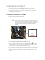
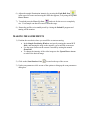
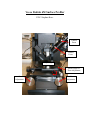
Veeco Dektak 6M Surface Profiler
POC: Stephan Koev
Camera
Zoom
Camera
Focus
Sample Stage
X
Rotate Stage for
Theta Adjustment
Y
Y
Adjustment
X
Adjustment
SYSTEM CHECK AND START UP
1) Turn on the monitor and start the Dektak32 application on the Desktop.
2) The system will initialize itself and will let you know when it is ready in the
bottom left corner of the screen.
LOADING/UNLOADING A SAMPLE
1) Load your sample on the positioning stage.
NOTE: The profiler is set up such that the scan is performed from front
to back on the stage (left to right on the monitor); therefore it is
necessary to place your sample on the stage at a rotated angle of
90 degrees so that the bottom of your sample is facing the
monitor.
Monitor
Scan
Scan
2) Press the Sample Positioning Window Icon,
, at the top.
3) Once your sample is positioned click on the Tower Down Icon,
, located at
the top of the screen. The tower and stylus assembly will move down to your
sample, touch the surface, and then the needle will rise up.
4) A video image of the sample will appear on the screen as the tower moves down.
5) Adjust the zoom and focus knobs on the sample viewing microscope for best
results.
6) Adjust the sample illumination intensity by pressing the Light Bulb Icon,
,
in the upper left corner and moving the slider that appears, or by using the Up and
Down Arrows
7) To unload press the Tower Up Icon,
, and wait for the tower to completely
rise. Your sample can then be removed from the stage.
8) Return the profiler to its standby mode by closing the Dektak32 program and
turning off the monitor.
MAKING MEASUREMENTS
1) Position the cross hairs where you would like to start measuring.
• In the Sample Positioning Window, navigate by turning the manual X-Y
Dials and rotating the stage to the structure you would like to measure.
• Use the zoom feature on the camera if needed by turning the manual
Zoom Dial.
• To change the intensity of the video image use the Up and Down Arrows
to achieve the desired image.
2) Click on the Scan Routines Icon,
, located at the top of the screen.
3) Under scan parameters click on one of the options to bring up the scan parameters
dialog box.
¾ Input the variables based on your sample and preferences:
Stylus type: Leave at 12.5um unless installing a new tip!
Length: scan length desired.
Duration: Enter the duration of the scan depending on the accuracy you need.
The number of sampling points based on this time will be shown in the
next box.
Resolution: resolution desired.
Scan types: Leave on standard scan.
Stylus force: Set between 1-15 mg. If measuring resist it should be between 1-3
mg.
Measurement range: Can be set from between 6.5um and 1mm.
Profile: select hills, valleys, or hills and valleys.
4) Once all variables are set select “OK” and then click on the Sample Positioning
Icon,
, on the top of the screen.
5) Adjust the measurement location if necessary and then hit the Run Current Scan
Routine Icon,
.
6) If there is a problem during the scan you can either hit “Escape” or press the
icon at the top of the screen.
TRACE ANALYSIS
1) Trace Leveling
• After the measurement is complete the program will bring you to the
Dataplot Screen.
• The cursors are labeled as “R” and “M” corresponding to Reference and
Measurement respectively.
• Place the cursors in the positions you would like the plot to be leveled by
dragging them with the mouse.
• If you would like the leveling to be done over a range of data points near
each cursor then click on the bottom of the cursor and expand the
bandwidth.
•
Hit F8 or the Leveling Icon,
2) Average Step Height Measurement
, to level the plot.
•
•
•
Place the Measurement Cursor over the section of the plot to measure and
the average step height will be displayed on the bottom right of the screen
under ASH.
A summary of the data will also be displayed in this area including:
Reference cursor position and width, Measurement cursor position and
width, average step height, and the distance between the cursors.
If you would like to store the average step height hit F12 and it will
appear on the left hand side of the screen under Analytic Results. The
individual results can be deleted by selecting them and hitting Delete.
3) Analytical Functions
•
•
•
•
When in the dataplot screen press the Calculator Icon,
, or click on
the analysis menu and select analytical functions.
In the dialog box that appears it is possible to select multiple parameters to
calculate including: roughness, height, waviness, and geometry.
Hit Compute to finish the calculation.
More details on this function can be found in the user’s manual.
EXPORTING DATA
1) In the dataplot view, click on the file menu and select Export.
• Save the data as Scan Data unless you are creating an auto-program which
can be found in the user’s manual.
• Select if it should be saved as either Tab Delimitated or Comma
Delimitated.
• Select if you would like to Overwrite the existing file or Append the data
to an existing text file.
Any further questions regarding the use of this tool that are not covered in
this SOP or the users manual should be brought to the attention of the POC.