Download User Manual - Automatic Control Group

User Manual
1
SUMMARY
Introduction .......................................................................................................................................... 3
Software structure ................................................................................................................................ 4
Installation ......................................................................................................................................... 5
Functionality of PNetLab simulator..................................................................................................... 6
Starting PNetLab simulator.................................................................................................................. 7
Drawing a Petri Net.............................................................................................................................. 9
Setting parameters .............................................................................................................................. 11
Parameters for place-transition Petri Nets ..................................................................................... 11
Parameters for Coloured Petri Nets with guard ............................................................................. 13
Parameters for Coloured Petri Nets without guard ........................................................................ 16
Parameters for Coloured Modified Hybrid Petri Nets ................................................................... 18
Parameters and function syntax of PNetLab simulator ...................................................................... 21
Examples ........................................................................................................................................ 23
Compiling a Petri Net ........................................................................................................................ 40
Simulation of a Petri Net .................................................................................................................... 41
Analysis of a PetriNet properties ....................................................................................................... 47
Including a control algorithm ............................................................................................................. 51
Example ............................................................................................................................................. 57
Introduction .......................................................................................................................................... 3
Software structure ................................................................................................................................ 4
Installation ......................................................................................................................................... 5
Functionality of PNetLab simulator..................................................................................................... 6
Starting PNetLab simulator.................................................................................................................. 7
Drawing a Petri Net.............................................................................................................................. 9
Setting parameters .............................................................................................................................. 11
Parameters for place-transition Petri Nets ..................................................................................... 11
Parameters for Coloured Petri Nets with guard ............................................................................. 13
Parameters for Coloured Petri Nets without guard ........................................................................ 16
Parameters for Coloured Modified Hybrid Petri Nets ................................................................... 18
Parameters and function syntax of PNetLab simulator ...................................................................... 21
Examples ........................................................................................................................................ 23
Compiling a Petri Net ........................................................................................................................ 40
Simulation of a Petri Net .................................................................................................................... 41
Analysis of a PetriNet properties ....................................................................................................... 47
Including a control algorithm ............................................................................................................. 51
Example ............................................................................................................................................. 57
2
Introduction
PNetLab is a software for Petri Nets (PN) simulation, analysis and supervision.
PNetLab allows modelling and analysis of Coloured Modified Hybrid Petri Nets (CMHPNs),
Coloured Petri Nets (CPNs), place-transition nets, timed/untimed.
The simulation engine has been developed in C++, it works in cooperation with a graphical user
interface and provides interactive simulation with graphical animation of the model and movement
of the tokens, step-by-step and off-line simulations, forward and backward time progression. It
allows drawing of timed/untimed, PN/CPN/CMHPN plant models by means a Java graphical user
interface.
For PN models (not for CPNs neither for CMHPNs), the computation of T-P-invariant, minimal
siphons and traps, pre-incidence, post-incidence and incidence matrixes and coverability tree is
available.
PNetLab allows the integration of a PN/CPN/CMHPN model with a standard C/C++ control
algorithm thus allowing closed-loop analysis and simulation of supervised systems. It is also
interfaced with Xpressby Dask Optimization, a tool of linear programming.
The simulation engine, without graphical interface, can be linked to an external program. This
allows the integration of PNetLab simulation engine in a general-purpose simulation loop.
3
Software structure
PNetLab software consists of a directory called PNetLab and a set of sub-directories:
•
GUI, it contains files related to the graphical user interface;
•
Engine, it contains files related to the simulation engine;
•
win32pad, it contains a text editor to visualize in textual form Petri Net properties that
simulator can analyse;
•
Examples, it contains several demonstrative Petri Net models.
In PNetLab directory we can find the file:PNetLab.bat,to start manually the simulator.
4
Installation
The simulator runs under Microsoft Windows XP, Windows Vista and Windows Seven
operating system.
The installation program starts by launching the file setup_v4_0.exe.
The simulator requires the following freeware software installation to work correctly:
-
Java 2 SDK, Standard Edition 1.4.1_01 or following versions
(www.java.sun/j2se/1.4.2/.);
-
Microsoft Visual C++ 2010 Express
-Crimson Editor
You can download it from official web sitewww.crimsoneditor.com. During the installation
set
C:\Program
Files\PNetLab\Crimson
Editor
as
destination
directory
or
C:name_of_directory_where_PNetLab_has_been_installed\Crimson Editor if PNetLab has been
installed in a directory different from C:\Program Files\PNetLab.
Please refer to readme.txt file, to obtain more details instruction about the installation of
PNetLab simulator.
5
Functionality of PNetLab simulator
PNetLab simulator allows you to execute the following operations:
•
draw a Petri Net;
•
simulate a Petri Net:
o in Off-Line mode (for any Petri Net);
o in Step by Step mode (only for not timed Petri Nets);
•
analysis of Petri Net (not available for CPNs neither for CMHPNs) by means of:
o coverability tree;
o P-invariants;
o T-invariants;
o siphons;
o traps.
6
Starting PNetLab simulator
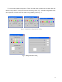
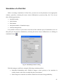
The simulator starts by launching the filePNetLab.bat. Firstly, a program presentation
window is opened (Fig. 1); it must be closed to use the simulator.
Fig. 1 – PnetLab presentation window
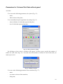
Then the type of Petri Net has to be chose (Fig. 2); once operating and confirming a choice, this
window closes and the selected editor starts.
Fig. 2 – Petri Net type selection window
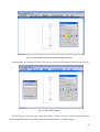
The main window is shown inFig. 3. It allows both to open a previously saved file and to create
a new one (this operations are available from the menu FileNew and FileOpen or from this
correspondent buttons
and
).
Fig. 3 – PNetLab toolbar
7
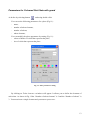
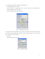
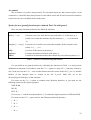
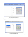
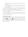
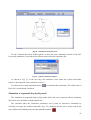
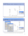
You can set the graphical properties of Petri Net nodes (this operations are available from the
menus SettingsPlace, SettingsTransition and SettingsArc, Fig. 4) and the background colour
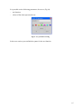
(this operation is available from the menu SettingsBackground, Fig. 5).
Fig. 4 – Graphical Petri Net properties setting
Fig. 5– Background colour setting
8
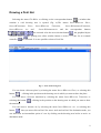
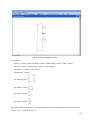
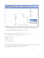
Drawing a Petri Net
Selecting the menu FileNew or clicking on the correspondent button
a window that
contains a void drawing area is opened (Fig. 6).The menus InsertDiscrete Place,
InsertContinuous
InsertDiscrete
InsertDiscrete
Place,
Arc
and
Transition,
InsertContinuousArc
and
InsertContinuousTransition,
the
are activated. Also the area selection button
selection button
controller
correspondent
buttons
, the graphical object
, the opening text editor window button to write C++ code for an eventual
are activated. It is now possible to draw a Petri Net.
Fig. 6 – Petri Net drawing area
You can insert a discrete place by selecting the menu InsertDiscrete Place, or selecting this
button,
; clicking in the position on the drawing area in which you want to draw the place.
You can insert a discrete transition by selecting the menu InsertDiscrete Transition, or
selecting this button,
; clicking in the position on the drawing area in which you want to draw
the transition.
You can insert a discrete arc by selecting the menu InsertDiscrete Arc, or selecting this
button
then you must click on Petri Net source node and on Petri Net destination node; you
can insert also an intermediate point of a arc by clicking on the drawing area before to arrive to
destination node.
9
You can insert a continuous place by selecting the menu InsertContinuous Place, or selecting
this button,
; clicking in the position on the drawing area in which you want to draw the place.
You can insert a continuous transition by selecting the menu InsertContinuous Transition, or
selecting this button,
; clicking in the position on the drawing area in which you want to draw
the transition.
You can insert a continuous arc by selecting the menu InsertContinuous Arc, or selecting this
button
then you must click on Petri Net source node and on Petri Net destination node; you
can insert also an intermediate point of a arc by clicking on the drawing area before to arrive to
destination node.
You can move the Petri Net nodes or an arc intermediate points by selecting this button
and
dragging the object that you want to move.
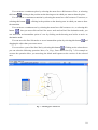
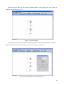
You can select a part of the Petri Net by selecting this button
.Clicking on the selected area
you can select the following operation: Move, Cut, Copy, Paste and Delete (Fig. 7). For example to
execute the operation Move you must drag the black small squares at the vertices of the selected
area.
Fig. 7 – Selecting part of Petri Net
10
Setting parameters
After drawing the net, it is possible to set the parameters for Place, Transition and Arc. These
parameters are different, in relation of the type of net you are analysing.
Parameters for place-transition Petri Nets
You can set the parameters of the places, transitions and arcs by selecting button
and
using double click on the object that you want to set; a window will appear in which you can
execute this operations.
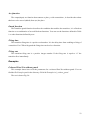
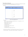
You can set the following parameters for a place (Fig. 8):
-
name;
-
number of tokens;
You can modify the place appearance by setting (Fig. 8):
-
colour of border of circle that represent the place;
-
size of circle that represent the place.
Fig. 8 – Place parameters setting
You can set this parameters for a transition (Fig. 9):
-
name;
-
firing time;
-
firing rate;
11
You can modify the transition appearance by setting (Fig. 9):
-
orientation (horizontal or vertical);
-
colour of filling (for a logical transition) or colour of border (for a timed transition) of
rectangle that represent the transition;
-
size of rectangle that represent the transition.
Fig. 9– Transition parameters setting
You can also modify the transition orientation by selecting the transition insertion button and
clicking on the transition that you want to rotate.
It is possible set the following parameters for an arc (Fig. 10):
-
arc weight;
-
colour of line that represent the arc.
Fig. 10 – Arc parameters setting
12
Parameters for Coloured Petri Nets with guard
As before by selecting button
and using double click:
You can set the following parameters for a place (Fig.11):
-
name;
-
number of token elements;
-
number of tokens;
-
token elements;
You can modify the place appearance by setting (Fig. 11):
-
colour of border of circle that represent the place;
-
size of circle that represent the place.
Fig. 11– Place parameters setting
By clicking on Token elements a windows will appear. It allows you to define the elements of
each token. As shown in Fig. 12the “Number of token elements” is 2 and the “Number of tokens” is
3 . You must insert a single element and you must to press enter.
13
Fig. 12– Token elements
You can set the following parameters for a transition (Fig.13):
-
name;
-
guard;
-
firing time;
-
firing rate;
You can modify the transition appearance by setting (Fig. 13):
-
orientation (horizontal or vertical);
-
colour of filling (for a logical transition) or colour of border (for a timed transition) of
rectangle that represent the transition;
-
size of rectangle that represent the transition.
Fig. 13– Transition parameters setting
14
It is possible set the following parameters for an arc (Fig.14):
-
arc function;
-
colour of line that represent the arc.
Fig.14– Arc parameters setting
In the next session you can find the syntax for the arc function.
15
Parameters for Coloured Petri Nets without guard
As before:
You can set the following parameters for a place (Fig. 15):
-
name;
-
token colours of the place;
You can modify the place appearance by setting (Fig. 15):
-
colour of border of circle that represent the place;
-
size of circle that represent the place.
Fig. 15– Place parameters setting
By clicking on Insert tokens a windows will appear. It allows you to specify the number of
tokens for each colour (Fig. 16). You must insert the number of tokens for each colour and you
must to press enter.
Fig. 16– Number of tokens
You can set the following parameters for a transition (Fig. 17):
-
name;
-
occurrence colours of the transition;
-
firing time;
16
You can modify the transition appearance by setting (Fig. 17):
-
orientation (horizontal or vertical);
-
colour of filling (for a logical transition) or colour of border (for a timed transition) of
rectangle that represent the transition;
-
size of rectangle that represent the transition.
Fig. 17– Transition parameters setting
You can set the following parameters for an arc(Fig. 18)only after you have set the parameters
of the place and of the transition which the arc links. You must to press enter after you have
insert each element of the arc matrix.
-
arc matrix;
-
colour of line that represent the arc.
Fig. 18– Arc parameters setting
17
Parameters for Coloured Modified Hybrid Petri Nets
As before:
You can set the following parameters for both discrete and continuous places (Fig. 19):
-
name;
-
token colors of the place;
As more, for a continuous place you can set the number of attributes in the marking, using the
windows circled in red in Fig. 19.b.
You can modify the place appearance by setting (Fig. 19 – Place parameters setting ( a-discrete
place; b-continuous place)):
-
colour of border of circle that represent the place;
-
size of circle that represent the place.
Fig. 19 – Place parameters setting ( a-discrete place; b-continuous place)
By clicking on Insert tokens a windows will appear. It allows you to specify the number of
tokens for each colour (Fig. 20). You must insert the number of tokens for each colour and you
must to press enter. For marking of continuous places having more than one attribute, values of
attribute have to be separated with a “,” (coma).
Fig. 20– Number of tokens
18
You can set the following parameters both for discrete and continuous transitions (Fig. 21):
-
name;
-
occurrence colours of the transition;
For discrete transition you also can set the:
-
firing time (Fig. 21.a).
As more for continuous transitions you can set:
-
type of the firing speed (0 depending by continuous place marking, 1 in the linear form
Ax+Bu, where x is the marking of the place having an arc entering in the transition; u is an
input value; A and B are matrices inserted by the user) (Fig. 22.b).
You can modify the transition appearance by setting (Fig. 21):
-
orientation (horizontal or vertical);
-
colour of filling (for a logical transition) or colour of border (for a timed transition) of
rectangle that represent the transition;
-
size of rectangle that represent the transition.
Fig. 21– Transition parameters setting (a- discrete transition; b-continuous transition)
19
Fig. 22 Firing speed setting: a- speed depending by the place marking; b – linear speed.
You can set the following parameters for both discrete and continuous arcs (Fig. 23) only after
you have set the parameters of the place and of the transition which the arc links. You must to
press enter after you have insert each element of the arc matrix.
-
arc matrix;
-
colour of line that represent the arc.
Fig. 23 – Arc parameters setting
20
Parameters and function syntax of PNetLab simulator
Since the simulator has not a syntactic interpreter, you must respect some simple rules to
correctly write the parameters of the drawn places, transitions and arcs, the guard functions, the arc
functions.
Before analyse in detail all the parameters you can set, it can be useful to list the main functions,
with a brief description of their operating mode and their syntax for a correct use.
Place(transition) name
The place(transition) name is a simple text label, so you must not follow any rule for it. You can
also associate a comment label to the place pi (transition ti); in this case next to the place pi
(transition ti) the following label is shown: pi-label (ti-label).
Token colours of the place and occurrence colours of the transition
Both token colours of the place and occurrence transition colour must be inserted as strings.
They allow to define both the token colours number and the occurrence colours themselves. It is
possible by simply writing the string of the colours separated by line space. Colours must by
integers.
Number of token elements
The number of token elements is a natural integer number. It defines the size of each token that
stays in the place.
Number of tokens
The number of tokens is a natural integer number.
Token elements
The token elements are integer numbers. They define the elements of each token.
Arc weight
The arc weight is always a positive integer number.
21
Arc matrix
The arc matrix is a positive integer matrix. For an output (input) arc that connect a place p with
a transition t, it describes how many tokens for each token colour and for each occurrence transition
colour has to be moved (added) from (to) the place.
Syntax for arc (guard) functions for coloured Petri Net with guard
There are many functions defined in the PNetLab simulator:
{c1, …,cN}
It builds the token (c1, …, cN).
pr(I, c1, …, ck)
Function projection; from the first reversed token <t> of the place pi it
builds a new token that contains only the elements c1, …, ck of the token
<t>.
conc[<t1>; …;<tN>]
Function link; it builds a new token that contains all the elements of the
tokens <t1>, …, <tN>.
All(i)
It selects all the tokens of the place pi.
ntoken(i)
It returns the number of tokens of the place pi.
BW(k)
It builds k decolourated tokens that contain only one element equals to (1).
Table 1 – Syntax for arc functions and guard functions
You can build an arc (guard) function by combining the functions in Table 1 or using several
mathematical functions in accordance with the C/C++ syntax or using C/C++ functions written by
user. In the last case the C/C++ code for this function must be written in the file F_user.ccp and the
headers of this function must be written in the file F_user.h. Both files are in the
directoryEngine/SimEngine of the simulator.
You must use the C/C++ syntax to combine more Boolean functions, so you must use the
following syntax for the logical operators:
AND &&
OR ||
NOT !
You can use “!” and the round parenthesis “()”to obtain the logical operators NAND and NOR.
You must use the C/C++ syntax also for the following relational operators:
= ==
≠ !=
≥ >=
≤ <=
22
Arc function
The output(input) arc function that connects a place p with a transition t, it describes the tokens
that have to be moved (added) from (to) the place.
Guard function
The transition guard function describes the condition that enables the transition, it is a Boolean
function or a combination of several Boolean functions. You can use the functions defined in Table
1 or other functions defined by user.
Firing time
The transition firing time is a positive real number. It is the delay time from enabling to firing of
a transition. For CPNs with guard the firing time can be also a function.
Firing rate
The transition firing rate is a positive integer number. If the firing rate is equal to “0” the
transition fires immediately.
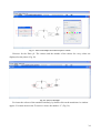
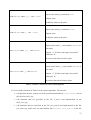
Examples
Coloured Petri Net without guard
This example shows how to set the parameters for a coloured Petri Net without guard. You can
find the file Example.pnml in the directory PNetLab/Examples/col_without_guard.
The net is shown Fig. 24:
23
Fig. 24 – Petri Net Example: draw net
Let suppose:
-
Place p1: colour 1 with 10 tokens; colour 2 with 8 tokens; colour 3 with 5 tokens.
-
Place p2: colour 1 with 0 tokens; colour 3 with 0 tokens.
-
Transition t1: colour 1 and colour 2.
-
Transition t2: colour 1.
-
1

Arc matrix p1t1: 1
0

-
0 1
Arc matrix t1p2: 
.
1 0
-
1 
Arc matrix p2t2:   .
2 
-
3
 
Arc matrix t2p1: 1 .
1
 
2

1.
2 
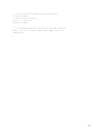
By double click on the Place p1 a window appears and you must write in the Token colours the
string “1 2 3” as shown in Fig. 25:
24
Fig. 25 – Petri Net Example: insert token colors
Subsequently by clicking on Insert tokens you can insert the number of the tokens for every
colour (Fig. 26).
Fig. 26– Petri Net Example: insert tokens
25
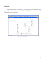
Likewise for the Place p2. The colours and the number of the tokens for every colour are
displayed on the places (Fig. 27).
Fig. 27 – Petri Net Example
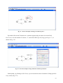
For insert the colours of the transition similarly, by double click on the transition t1 a window
appear. You must insert in the Transition colours the string “1 2” (Fig. 28).
Fig. 28– Petri Net Example: insert transition colures
26
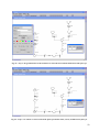
Likewise for transition t2. To insert the arc matrix you must to do a double click on one of the
middle points. A window appears that contains a matrix of zeros and you must insert there the
correspondently arc matrix. The following figure shows as insert the arc matrix for the Arc p1t1.
Fig. 29 – Petri Net Example: insert arc matrix
This operation has to be done for every arc of the net. Only after you have set the parameters for
the whole net, you can compile and you can execute the simulation. These operation are shown in
the next sessions.
27
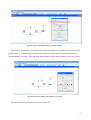
Coloured Petri Net with guard
This example shows how to set the parameters for a coloured Petri Net with guard. You can find
the file Example1.pnml in the directory PNetLab/Examples/col_with_guard.
The net is:
Fig. 30 – Petri Net Example1: draw net
Let suppose:
-
Place p1: 2 tokens with 3 elements, in particular: token 1={1,7,8} and token 2={2,7,8}.
-
Place p2: 0 tokens, with 2 elements.
-
Transition guard t1: pr(1,1)==2.
-
Transition guard t2: pr(2,2)==7.
-
Arc function p1t1: 1.
-
Arc function t1p2: conc[pr(1,1); pr(1,2)].
-
Arc function p2t2: 1.
-
Arc function t2p1: conc[pr(2,1); pr(2,2); {8}].
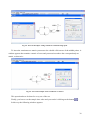
By double click on the Place p1 a window appears and you must write in Number of token
elements the number “3”and in Number of tokens the number “2”as shown in Fig. 31:
28
Fig. 31 – insert number of token elements and number of tokens
Subsequently by clicking on Token elements you can insert all elements of each token (Fig. 32).
Fig. 32 – insert token elements
For the Place p2 you must insert only the Number of token elements. After you must insert the
transition guard function, by double clicking on the transition t1 a window appear:
29
Fig. 33 – transition t1 guard function
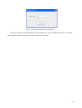
Likewise for transition t2. Finally, to insert the arc function you must to do a double click on the
middle point of an arc and a window appear. In this window you can write the appropriate function.
The following figure shows as insert the arc matrix for the Arc t2p1:
Fig. 34 –insert arc function
30
This operation has to be done for every arc of the net. The arc function is displayed next to the
middle point of the arc. Only after you have set the parameters for the whole net, you can compile
and you can execute the simulation. These operation are shown in the next sessions.
31
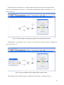
Coloured Modified Hybrid Petri Net
This example shows how to set the parameters for a Coloured Modified Hybrid Petri Net.
The net is:
Fig. 35 – Petri Net Example: draw net
Let suppose:
Discrete places:
-
Place p1: 2 colours; token number of colour 1 = 1; token number of colour 2 = 1.
-
Place p2: 2 colours; token number of colour 1 = 0; token number of colour 2 = 0.
Continuous place:
-
Place pc1: 2 coloured marking with 2 attributes;
values of attributes for colour 1 = <0.5 , 0.3>;
values of attributes for colour 2 = <0.8 , 0.9>;
Discrete Transitions:
-
Transition t1: 2 colours;
-
Transition t2: 2 colours;
Continuous Transitions:
-
Transition tc1: 2 colours; linear firing speed (Ax+Bu) with
0 1
0
, , u = 0.8
1 0
1
Discrete Arcs:
-
1
0
1
Arc t2p2: 0
Arc p1t2: 0
.
1
0
.
1
32
-
1
0
1
Arc t1p1: 0
Arc p2t1: 0
.
1
0
.
1
Continuous Arcs:
1,1 0
0
1,1 1,1 0
Arc p1tc1: 0
1,1 1,1 0
Arc tc1p1: 0
1,1 - Arc pc1tc1: -
By double click on the Place p1 a window appears and you must write in Token color the string “1
2”as shown in Fig. 31:
Fig. 36 – insert token colour for discrete places
Subsequently by clicking on Insert tokens you can insert the number of the tokens for every
colour (Fig. 37).
33
Fig. 37– Petri Net Example: insert discrete places’ tokens
Likewise for the Place p2. The colours and the number of the tokens for every colour are
displayed on the places (Fig. 38).
Fig. 38– Petri Net Example
For insert the colours of the transition similarly, by double click on the transition t1 a window
appear. You must insert in the Transition colours the number “2” (Fig. 39).
34
Fig. 39- Petri Net Example: discrete transition colours
Likewise for transition t2. To insert the arc matrix you must to do a double click on one of the
middle points. A window appears that contains a matrix of zeros and you must insert there the
correspondently arc matrix. The following figure shows as insert the arc matrix for the Arc p1t1.
Fig. 40–Petri Net Example: insert discrete arc matrix
This operation has to be done for every arc of the net.
35
By double click on the Place pc1 a window appears and you must write in the first field of
Token color the number of colours, “2”, and in the second filed the number of attributes, “2”, as
shown in Fig. 31:
Fig. 41– Petri Net Example: setting continuous place colours and attributes number.
Subsequently by clicking on Insert tokens you can insert the value of tokens’ attributes for
every colour (Fig. 37).
Fig. 42– Petri Net Example: setting continuous place attributes values.
The marking of the continuous place is displayed near the place, as shown in Fig. 38.
36
Fig. 43 – Petri Net Example: marking of continuous places.
By double click on the Transition tc1 a window appears and you must write in the field
Occurrence color the number of colours, “2”, and in the field Type the firing speed type “1”, as
shown in Fig. 312:
Fig. 44 – Petri Net Example: setting continuous transition parameters.
Subsequently by clicking on Set Velocity you can insert the value of transition’s firing speed for
every colour (Fig. 373).
37
Fig. 45– Petri Net Example: setting continuous transition firing speed.
To insert the continuous arc matrix you must to do a double click on one of the middle points. A
window appears that contains a matrix of zeros and you must insert there the correspondently arc
matrix, as shown in :
Fig. 46 – Petri Net Example: insert continuous arc matrix
This operation has to be done for every arc of the net.
Finally, you have to set the sample time value and you can do it clicking on the button
.
In this way the following windows appears:
38
Fig. 47 – Petri Net Example: insert sample time.
Only after you have set the parameters for the whole net, you can compile and you can execute
the simulation. These operation are shown in the next sessions.
39
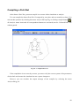
Compiling a Petri Net
After drawn a Petri Net, you must compile it to execute either simulation or analysis.
You can compile the drawn Petri Net if composed by one place and one transition at least. You
can run this operation by selecting the menu AnalysisCompiling or clicking compile button
,
all Analysis menu items and all correspondent buttons are activated (not for Coloured Petri Net
without guard).
Fig. 48 – A compiled Petri net
If the compilation is not correctly execute, you must verify the correct syntax of the parameters
of the whole net because the simulator has not a syntax interpreter.
However you can visualize the output message of the compiler by selecting the menu
AnalysisLog file.
40
Simulation of a Petri Net
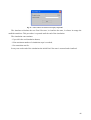
Before executing a simulation of a Petri Net, you must set several parameters in an appropriate
window, opened by selecting the menu AnalysisSimulation parameters(Fig. 49). You can set
these following parameters:
•
simulation mode;
•
initial instant;
•
final instant;
•
maximum number of simulation steps;
•
conflicts management;
It is possible to choose if you want to write the out files with the report of simulation or not. At
this point you can start the simulation by selecting the menu AnalysisSimulation or clicking on
simulation button
.
Fig. 49 –Simulation parameters setting
PNetLab manages conflicts by using the following resolution policies:
•
Predefined Scheduling order: PNetLab assigns a static priority to the transition in
conflict, based on the order in which they have been drawn;
•
Same firing rate: transition in conflict relation have the same firing probability;
41
•
Stochastic firing rate: transition in conflict relation have a firing probability defined a
priori by the user;
•
Controller: the subroutine Controller is called to solve the conflict, the conflict
resolution is charged to the user, who has the responsibility of programming the proper
conflict resolution policy.
If you don’t set the simulation parameters, you can start a simulation in Off-Line mode that lasts
maximum 1000 times units and maximum 100 simulation steps. The conflicts management is in
accordance with the Predefined Scheduling order and the output files will be written.
If you start a new simulation, the parameters of the old simulation will be valid if you don’t
modify the simulation parameters,.
You can execute a simulation in Off-Line mode or in Step-by-Step mode. You can also execute
the second one in sequential mode or in concurrent mode. In the next sub-sessions you can find
more information on the simulation mode.
Simulation in Off-Line mode
The Off-Line mode simulation allows you to execute a simulation without interaction. At the
end a simulation window is opened by which you can observe the Petri Net evolution by clicking on
forward button
or backward button
to visualize on the drawing area all the states that the
Petri Net assumes during the simulation. In the same simulation window you can read several useful
information such as the current simulation step, the current simulation time and the transition fired
in the precedent state (Fig. 50).
42
Fig. 50 – Simulation in Off-Line mode
For the Coloured Petri Nets without guard, we have the same simulation window in the OffLine mode simulation. It also shows the colours under which the transitions fire.
Fig. 51 – Off-Line simulation windows
As shown in Fig. 51, at the first step, the transition t1fires under the colourc1and under
colourc2, the transition t2fires under the colourc1.
You must click on stop simulation button
to terminate this simulation. The initial state of
Petri Net is restored and visualized.
Simulation in sequential Step-by-Step mode
The simulation in sequential Step-by-Step mode allows the user to interact with the simulator.
This mode is not available with the hybrid nets.
The simulator takes the simulation parameters and it starts an interactive simulation by
colouring in orange the enabled transitions (Fig. 52), disabling all the active menus and all the
active buttons and enabling only the end simulation button .
43
Fig. 52 – Simulation in sequential step-by-step mode
For both place-transition and Coloured Petri Nets with guard, you can choose which transition
to be fired simply by click; for the Coloured Petri Nets without guard, you must choose the colour
under which the transition fires. Clicking on the transition, you will see a windows showing the
enabled colours (Fig. 53).You can choose one of the enabled colours by click on the button “Ok”.
Fig. 53 – Select colours in sequential step-by-step mode
The simulator calculates the new Petri Net state, it visualizes the state and the new enabled
transitions are coloured in orange. This procedure is repeated till the end of the simulation.
The simulation can terminate:
- if you click the end simulation button;
- if the maximum number of simulation steps is reached;
- if no transition can fire.
In any case at the end of the simulation the initial Petri Net state is restored and it is visualized.
44
Simulation in concurrent Step-by-Step mode
The simulation in concurrent Step-by-Step mode allows the user to interact with the simulator.
This mode is not available with the hybrid nets.
It is possible that more transitions can fire simultaneously and a transitions can fire under more
colours simultaneously.
The simulator takes the simulation parameters and it starts an interactive simulation by
colouring in orange the enabled transitions, disabling all the active menus and all the active buttons
and enabling only the start simulation button
and the end simulation button .
You can now choose which transitions has to fire by selecting them; the simulator colours in red
these transitions (Fig. 54). They fire when you click on the start simulation button.
You can disable the transitions selected by clicking again.
Fig. 54 – Simulation in concurrent step-by-step mode
As described before, you must choose the colours under which the transitions fire for the
coloured Petri Nets without guard also. The transition becomes red only after you specify either the
colour or the colours, if more than one, under which the transition fires. You must select the colours
under which a transition fires and write them on the appropriate field separated by line space (Fig.
55). This operation should be done for any transition you want fire simultaneously when you click
on the start simulation button.
45
Fig. 55 – Select colours in concurrent step-by-step mode
The simulator calculates the new Petri Net state, it visualizes the state, it colours in orange the
enabled transitions. This procedure is repeated until the end of the simulation.
The simulation can terminate:
- if you click the end simulation button;
- if the maximum number of simulation steps is reached;
- if no transition can fire.
In any case at the end of the simulation the initial Petri Net state is restored and visualized.
46
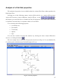
Analysis of a Petri Net properties
This analysis of properties is not available neither for coloured Petri Nets without guard nor for
Hybrid petri Nets.
Selecting one of this following menus, AnalysisCoverability tree, AnalysisP-invariants,
AnalysisT-invariants, AnalysisSiphons, AnalysisTraps, or one
of
this buttons, you can define how to calculate the Petri Net properties. The result of this calculation
is visualized, in textual form, in a separate window of a text editor.
You can analyse this following properties:
•
coverability tree;
•
P-invariants;
•
T-invariants;
•
siphons;
•
traps.
You can also visualize the Petri Net matrixes by selecting the menu AnalysisIncidence
matrixes, or clicking this button
.
The next example shows some Petri Net properties for the net in Fig. 56. You can find this file,
Cat_Mouse.pnml, in the directory PNetLab/Examples/P-T_net.
Fig. 56 – Petri Net properties
47
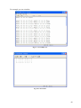
For example you can visualize:
Fig. 57– Coverability tree
Fig. 58– P-Invarinats
48
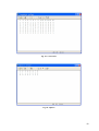
Fig. 59– T-Invarinats
Fig. 60– Siphons
49
Fig. 61– Traps
Fig. 62 – Pre, Post and Incidence matrices
50
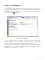
Including a control algorithm
PNetLab simulator allows you to execute a supervisory control policy of the Petri Net by a
controller, that is a control algorithm that disables several enabled transitions in accordance with a
control politics. You must write this algorithm in C++ in the file Controller.cpp. You can visualize
it by clicking this button
(Fig. 63).
Fig. 63 – Control algorithm writing
You must always write the control algorithm both in the file Controller.cpp and in the
predetermined method controller() of the C++ class Controller. You must never
modify the name and the position of this file so that the simulator can correctly run.
You can access to several information about the Petri Net state during the simulation to write a
control algorithm; you can also disable transitions and add/remove tokens from places. You can
perform these, using these following C++ functions.
51
int m(char *p_i)
Input: place name p_i.
Output: number of tokens of the place pi.
int m(int i)
Input: indexi of the place pi.
Output: number of tokens of the place pi.
Input: indexi and index j of the Petri Net
intmatInc(int i, int j)
incidence matrix (1≤i≤number_of_places,
1≤j≤number_of_transitions)
Output: element cij of the incidence matrix.
Input: none.
intnPosti()
Output: number of places of the Petri Net.
Input: none.
intnTrans()
Output: number of transitions of the Petri Net.
Input: place name p_i, index token i,index
intcompToken(char *p_i, int i, int j)
element j
Output: element j of the token i of the place pi.
Input: place index p_i, index token i, index
intcompToken(intp_i, int i, int j)
element j
Output: element j of the token i of the place pi.
52
Input: place name p_iand tokentoken.
voidaddToken(char *p_i, int *token)
Output: none.
It adds the token to the place.
Input: place index p_i and token token.
voidaddToken(intp_i, int *token)
Output: none.
It adds the token to the place.
Inputi: place name p_iand number idToken of
the token.
intdelToken(char *p_i, intidToken)
Output: “1” if token removing is successful,
otherwise “0”.
It removes the token from the place.
Inputi: place index p_i and number idToken of
the token.
intdelToken(intp_i, intidToken)
Output: “1” if token removing is successful,
otherwise “0”.
It removes the token from the place.
Table 2 – Usable C++ function to write a control algorithm
You can call the functions in Table 2 in the control algorithm. You can also:
•
call functions that are written out of the predetermined method controller(), but in
the file Controller.cpp;
•
call functions that are specified in the file F_user.h and implemented in the
fileF_user.cpp;
•
call functions that are specified in the file file_name.h and implemented in the file
file_name.cpp; in this case you must add the line #include “file_name.h” in the file
53
Controller.cpp. You must also add the files file_name.handfile_name.cpp in the
directory Engine/SimEngine(SimEngine_new) of simulator; finally you must modify the
file buildsim.bat in the directory Engine/SimEngine(SimEngine_new) of simulator in this
way:
cd..
cd Engine
cd SimEngine(SimEngine_new)
funz_arco
guardie
cl/c file_name.cpp
cl /c F_user.cpp
cl/c Controller.cpp
cl /c Simulatore.cpp
link /OUT:Simulatore.exe Simulatore.obj Simula.obj Arco.obj Trans.obj
Posto.obj
Rete.obj
eventlist.obj
Funzioni.obj
F_user.obj
RND.obj
file_name.obj Controller.obj
You must restore the original file buildsim.bat if you don’t want to include a control algorithm
anymore.
You must always compile the Petri Net to activate the written control algorithm.
After closing the program, the file Controller.cpp is stored in the directory Engine/SimEngine
(SimEngine_new); if you restart the simulator, the precedent file Controller.cpp is loaded when you
compile a new Petri Net and the control algorithm is applied to the simulation and the analysis of
the Petri Net. It may cause several unexpected behaviours or mis-functionalities of the simulator.
Then you must always verify that the file Controller.cppis correct.
In the following example, a control algorithm that uses the Xpress functions is shown. You can
find
this
control
algorithm
file
ControllerXpressExample.cpp,
in
the
directory
PNetLab/Examples/P-T_net/XpressExample, this algorithm enforces the behaviour of the Petri Net
XpressExample.pnml that you can find in the same directory.
54
Example:
#include <stdlib.h>
#include <stdio.h>
#include "Controller.h"
#include "Rete.h"
#include "Funzioni.h"
#include "F_user.h"
#include "mat_lib.h"
#include "prog_lint.h"
#include "xprs.h"
extern bool endContr; //End control algorithm
extern Rete r; //Petri Net
extern int *CV; //Vector transitions enabled
extern int **runtimeConflict; //Structural conflict transitions
extern bool *realConflict; //Real conflict transitions
void Controller::controller() {
intnrow, ncol, nvgmec=1, i, j;
nrow=nPosti();
// Number of places
ncol=nTrans();
// Number of transitions
// Define the incidence matrix C and initialize it
int **C=NULL;
C=dmat_int(nrow, ncol, 0);
// Define the constraint matrix Lgmec and initialize it
int **Lgmec=NULL;
Lgmec=dmat_int(nvgmec, nrow, 0);
//Build the incidence matrix C by using the PNetLab function matInc()
for (i=0; i<nrow; i++)
for (j=0; j<ncol; j++)
C[i][j]=matInc(i+1, j+1);
// Build the constraint matrix Lgmec
Lgmec[0][0]=1;
// Define vector Kgmec
intkgmec[]={2};
// In this example GMEC is m(1)<=1
// Definition of the vector utran which specifies the controllable and
// uncontrollable transitions, utran[i-1]=1 means that transition "ti" is uncontrollable
int *utran=NULL;
utran=dvet_int(ncol, 0);
utran[0]=1; utran[5]=1;
utran[6]=1; utran[7]=1;
55
// Load the current PN marking by using function m(i)
int *marcatura=NULL;
marcatura=dvet_int(nrow, 0);
for(i=1; i <= nrow; i++)
marcatura[i-1]=m(i);
// Call extern Xpress© function mpli that solve GMEC constraint
mpli(C, nrow, ncol, marcatura, Lgmec, kgmec, nvgmec, utran, CV);
endContr=true;
}
56
Example
In the following example, the simulation of a coloured timed Petri Net with guard is shown
(Fig.
64).
You
can
find
the
file
Example2.pnml
in
the
directory
PNetLab/Examples/col_with_guard.
Fig. 64– Petri Net Example2
57
Fig. 65 – Step 1: the guard function of the transition t1 selects the first and the third token of the place p1.
Fig. 66 – Step 2: two tokens are removed from the places p2 and the token (1,2,3,4) is added to the place p3.
58
Fig. 67– Step 3: the token (1,2,3,4) is removed from the place p3 and three tokens are added to the place p4
Fig. 68– Step 4: the arc function {0,3,0,0,2,0,0,1,0} adds three token to the place p5 if his token number of token
elements is equal to three
59
Fig. 69 – Step 5: the arc function pr(8,1,2,3) select the elements 1, 2, 3 of the token of the place p5
Fig. 70 – Step 6: the conflict among the transitions t6 and t7 is solved by using guard functions
60
Fig. 71– Step 7: the firing time of the transition t8 is a user function written in the file F_user.cpp
The user defines this following function in the file F_user.cpp:
/****************************************************************/
// function: double traveltime(int x, int y);
// it calculate the necessary time to reach the position {x,y}
// in accordance with the function max{x/Vx, y/Vy}.
double traveltime(int x, int y) {
double Vx = 50.5;
double Vy = 75.8;
double tx = x/Vx;
double ty = y/Vy;
if (tx>ty) return tx;
else return ty;
}
In this function the firing time of the transition t8 depends on the token colour of the place p8.
The following header of this function is written in the file F_user.h:
double traveltime(int x, int y);
61