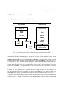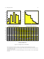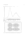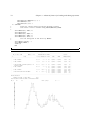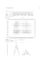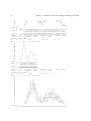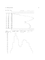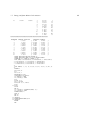
1
CERN Program Library Long Writeups Y250
HBOOK
Statistical Analysis and Histogramming
Reference Manual
Information Technology Division
CERN Geneva, Switzerland
Copyright Notice
HBOOK – Statistical Analysis and Histogramming
CERN Program Library entry Y250
c Copyright CERN, Geneva 1995–1998
Copyright and any other appropriate legal protection of these computer programs and associated
documentation reserved in all countries of the world.
These programs or documentation may not be reproduced by any method without prior written consent of the Director-General of CERN or his delegate.
Permission for the usage of any programs described herein is granted apriori to those scientific
institutes associated with the CERN experimental program or with whom CERN has concluded a
scientific collaboration agreement.
Requests for information should be addressed to:
CERN Program Library Office
CERN-IT Division
CH-1211 Geneva 23
Switzerland
Tel. +41 22 767 4951
Fax. +41 22 767 8630
Email: [email protected]
Trademark notice: All trademarks appearing in this guide are acknowledged as such.
Contact Person:
Olivier Couet /IT
([email protected])
Technical Realization:
Michel Goossens /IT
([email protected])
Edition – August 1998
Foreword
History
HBOOK is a Fortran1 callable package for histogramming and fitting. It was originally developed in the
1970s and has since undergone continuous evolution culminating in the current version, HBOOK 4.
Many people have contributed to the design and development of HBOOK, through discussions, comments and suggestions.
For many years and up to November 1994 René Brun has been responsible for the HBOOK program.
Paolo Palazzi was involved in the original design. D. Lienart has been in charge of the parametrization
part. Fred James is the author of routine HDIFF and of the minimization package Minuit, which forms the
basis of the fitting routines. The idea of Profile histograms has been taken from the HYDRA system. The
Column-wise-Ntuple routines were implemented by Fons Rademakers. The multi-dimensional quadratic
fit package HQUAD is the work of John Allison. J. Linnemann and his colleagues of the D0 experiment
contributed the routine HDIFFB. Pierre Aubert is the author of the routines to associate labels with
histograms. Roger Barlow and Christine Beeston (OPAL) have developed the HMCMLL package. Julian
Bunn is the author of the HNFORM routine.
Preliminary remarks
This manual serves at the same time as a Reference manual and as a User Guide for the HBOOK
system. After a short introductory chapter, where the basic ideas are explained, the following chapters
describe in detail the calling sequences for the different user routines.
In this test examples are in monotype face and strings to be input by the user are underlined. In the
index the page where a routine is defined is in bold, page numbers where a routine is referenced are in
normal type.
In the description of the routines a * following the name of a parameter indicates that this is an output
parameter. If another * precedes a parameter in the calling sequence, the parameter in question is both
an input and output parameter.
Some informations about HBOOK can also be found on the Web in the “PAW frequently asked questions” page
http://wwwinfo.cern.ch/asdcgi/listpawfaqs.pl
This document has been produced using LATEX [1] with the cernman style option, developed at CERN.
1
A C interface is also distributed by the CERN Program Library, created using the tool f2h
i
ii
Table of Contents
1 Introduction
1
1.1
Data processing flow in particle experiments . . . . . . . . . . . . . . . . . . . . . . . .
1
1.2
HBOOK and its output options . . . . . . . . . . . . . . . . . . . . . . . . . . . . . . .
2
1.3
What you should know before you start . . . . . . . . . . . . . . . . . . . . . . . . . .
3
1.3.1
HBOOK parameter conventions . . . . . . . . . . . . . . . . . . . . . . . . . .
4
1.4
A basic example . . . . . . . . . . . . . . . . . . . . . . . . . . . . . . . . . . . . . . .
5
1.5
HBOOK batch as the first step of the analysis . . . . . . . . . . . . . . . . . . . . . . .
8
1.5.1
1.6
Adding some data to the RZ file . . . . . . . . . . . . . . . . . . . . . . . . . .
11
HPLOT interface for high quality graphics . . . . . . . . . . . . . . . . . . . . . . . . .
13
2 One and two dimensional histograms – Basics
2.1
16
Booking . . . . . . . . . . . . . . . . . . . . . . . . . . . . . . . . . . . . . . . . . . .
16
2.1.1
One-dimensional case . . . . . . . . . . . . . . . . . . . . . . . . . . . . . . .
16
2.1.2
Two-dimensional case . . . . . . . . . . . . . . . . . . . . . . . . . . . . . . .
16
2.2
Filling . . . . . . . . . . . . . . . . . . . . . . . . . . . . . . . . . . . . . . . . . . . .
17
2.3
Editing . . . . . . . . . . . . . . . . . . . . . . . . . . . . . . . . . . . . . . . . . . . .
18
2.4
Copy, rename, reset and delete . . . . . . . . . . . . . . . . . . . . . . . . . . . . . . .
18
3 Ntuples
20
3.1
CWN and RWN – Two kinds of Ntuples . . . . . . . . . . . . . . . . . . . . . . . . . .
20
3.2
Row-Wise-Ntuples (RWN) . . . . . . . . . . . . . . . . . . . . . . . . . . . . . . . . .
22
3.2.1
Booking a RWN . . . . . . . . . . . . . . . . . . . . . . . . . . . . . . . . . .
22
3.2.2
Filling a RWN . . . . . . . . . . . . . . . . . . . . . . . . . . . . . . . . . . .
22
More general Ntuples: Column-Wise-Ntuples (CWN) . . . . . . . . . . . . . . . . . . .
25
3.3.1
Booking a CWN . . . . . . . . . . . . . . . . . . . . . . . . . . . . . . . . . .
26
3.3.2
Describing the columns of a CWN . . . . . . . . . . . . . . . . . . . . . . . . .
27
3.3.3
Creating CHFORM dynamically . . . . . . . . . . . . . . . . . . . . . . . . . . .
29
3.3.4
Filling a CWN . . . . . . . . . . . . . . . . . . . . . . . . . . . . . . . . . . .
31
3.4
Making projections of a RWN . . . . . . . . . . . . . . . . . . . . . . . . . . . . . . .
33
3.5
Get information about an Ntuple . . . . . . . . . . . . . . . . . . . . . . . . . . . . . .
35
3.5.1
Retrieve the contents of a RWN into an array . . . . . . . . . . . . . . . . . . .
35
3.5.2
Retrieve the contents of a CWN into a common block . . . . . . . . . . . . . . .
37
3.5.3
Generate a user function . . . . . . . . . . . . . . . . . . . . . . . . . . . . . .
39
3.5.4
Optimizing event loops . . . . . . . . . . . . . . . . . . . . . . . . . . . . . . .
41
3.6
Ntuple operations . . . . . . . . . . . . . . . . . . . . . . . . . . . . . . . . . . . . . .
41
3.7
Ntuple examples . . . . . . . . . . . . . . . . . . . . . . . . . . . . . . . . . . . . . .
43
3.3
iii
4 Advanced features for booking and editing operations
4.1 Overview of booking options . . . . . . . . . . . . . . . . . . . . . . . . . . . . . . . .
4.1.1 Histograms with non-equidistant bins . . . . . . . . . . . . . . . . . . . . . . .
54
54
54
4.1.2
4.1.3
Profile histograms . . . . . . . . . . . . . . . . . . . . . . . . . . . . . . . . .
Rounding . . . . . . . . . . . . . . . . . . . . . . . . . . . . . . . . . . . . . .
54
55
4.1.4
4.1.5
Projections, Slices, Bands . . . . . . . . . . . . . . . . . . . . . . . . . . . . .
Statistics . . . . . . . . . . . . . . . . . . . . . . . . . . . . . . . . . . . . . .
55
57
4.1.6
4.1.7
Function Representation . . . . . . . . . . . . . . . . . . . . . . . . . . . . . .
Reserve array in memory . . . . . . . . . . . . . . . . . . . . . . . . . . . . . .
57
59
4.1.8 Axis labels and histograms . . . . . . . . . . . . . . . . . . . . . . . . . . . . .
Filling Operations . . . . . . . . . . . . . . . . . . . . . . . . . . . . . . . . . . . . . .
4.2.1 Fast Filling Entries . . . . . . . . . . . . . . . . . . . . . . . . . . . . . . . . .
59
60
60
4.2.2
4.2.3
Global Filling . . . . . . . . . . . . . . . . . . . . . . . . . . . . . . . . . . . .
Filling histograms using character variables . . . . . . . . . . . . . . . . . . . .
63
64
Editing operations . . . . . . . . . . . . . . . . . . . . . . . . . . . . . . . . . . . . . .
4.3.1 Index and General Title . . . . . . . . . . . . . . . . . . . . . . . . . . . . . . .
78
79
4.3.2
4.3.3
4.3.4
What to Print (1-dimensional histogram) . . . . . . . . . . . . . . . . . . . . .
Graphic Choices (1-dimensional histogram) . . . . . . . . . . . . . . . . . . . .
Scale Definition and Normalization . . . . . . . . . . . . . . . . . . . . . . . .
80
82
83
4.3.5
4.3.6
Page Control . . . . . . . . . . . . . . . . . . . . . . . . . . . . . . . . . . . .
Selective Editing . . . . . . . . . . . . . . . . . . . . . . . . . . . . . . . . . .
85
85
4.3.7
4.3.8
Printing after System Error Recovery . . . . . . . . . . . . . . . . . . . . . . .
Changing Logical unit numbers for output and message files . . . . . . . . . . .
87
87
5 Accessing Information
5.1 Testing if a histogram exists in memory . . . . . . . . . . . . . . . . . . . . . . . . . .
5.2 Testing if a ntuple is a RWN or a CWN . . . . . . . . . . . . . . . . . . . . . . . . . .
93
93
93
4.2
4.3
5.3
5.4
List of histograms . . . . . . . . . . . . . . . . . . . . . . . . . . . . . . . . . . . . . .
Number of entries . . . . . . . . . . . . . . . . . . . . . . . . . . . . . . . . . . . . . .
93
94
5.5
5.6
Histrogram attributes Contents . . . . . . . . . . . . . . . . . . . . . . . . . . . . . . .
Contents . . . . . . . . . . . . . . . . . . . . . . . . . . . . . . . . . . . . . . . . . . .
94
95
5.7
5.8
Errors . . . . . . . . . . . . . . . . . . . . . . . . . . . . . . . . . . . . . . . . . . . .
Associated function . . . . . . . . . . . . . . . . . . . . . . . . . . . . . . . . . . . . .
96
98
5.9 Abscissa to channel number . . . . . . . . . . . . . . . . . . . . . . . . . . . . . . . .
5.10 Maximum and Minimum . . . . . . . . . . . . . . . . . . . . . . . . . . . . . . . . . .
5.11 Rebinning . . . . . . . . . . . . . . . . . . . . . . . . . . . . . . . . . . . . . . . . . .
98
99
99
5.12 Integrated contents . . . . . . . . . . . . . . . . . . . . . . . . . . . . . . . . . . . . . 100
5.13 Histogram definition . . . . . . . . . . . . . . . . . . . . . . . . . . . . . . . . . . . . 100
5.14 Statistics . . . . . . . . . . . . . . . . . . . . . . . . . . . . . . . . . . . . . . . . . . . 101
iv
6 Operations on Histograms
102
6.1
Arithmetic Operations
6.2
Statistical differences between histograms . . . . . . . . . . . . . . . . . . . . . . . . . 103
6.3
. . . . . . . . . . . . . . . . . . . . . . . . . . . . . . . . . . . 102
6.2.1
Weights and Saturation . . . . . . . . . . . . . . . . . . . . . . . . . . . . . . . 104
6.2.2
Statistical Considerations . . . . . . . . . . . . . . . . . . . . . . . . . . . . . . 104
Bin by bin histogram comparisons . . . . . . . . . . . . . . . . . . . . . . . . . . . . . 106
6.3.1
Choice of TOL: . . . . . . . . . . . . . . . . . . . . . . . . . . . . . . . . . . . 108
7 Fitting, parameterization and smoothing
7.1
7.2
112
Fitting . . . . . . . . . . . . . . . . . . . . . . . . . . . . . . . . . . . . . . . . . . . . 112
7.1.1
One and two-dimensional distributions . . . . . . . . . . . . . . . . . . . . . . 113
7.1.2
Fitting one-dimensional histograms with special functions . . . . . . . . . . . . 114
7.1.3
Fitting one or multi-demensional arrays . . . . . . . . . . . . . . . . . . . . . . 115
7.1.4
Results of the fit . . . . . . . . . . . . . . . . . . . . . . . . . . . . . . . . . . 116
7.1.5
The user parametric function . . . . . . . . . . . . . . . . . . . . . . . . . . . . 117
Basic concepts of MINUIT . . . . . . . . . . . . . . . . . . . . . . . . . . . . . . . . . 118
7.2.1
Basic concepts - The transformation for parameters with limits. . . . . . . . . . 118
7.2.2
How to get the right answer from MINUIT . . . . . . . . . . . . . . . . . . . . 119
7.2.3
Interpretation of Parameter Errors: . . . . . . . . . . . . . . . . . . . . . . . . . 119
7.2.4
MINUIT interactive mode . . . . . . . . . . . . . . . . . . . . . . . . . . . . . 121
7.3
Deprecated fitting routines . . . . . . . . . . . . . . . . . . . . . . . . . . . . . . . . . 124
7.4
Parametrization . . . . . . . . . . . . . . . . . . . . . . . . . . . . . . . . . . . . . . . 125
7.5
Smoothing . . . . . . . . . . . . . . . . . . . . . . . . . . . . . . . . . . . . . . . . . . 131
7.6
Random Number Generation . . . . . . . . . . . . . . . . . . . . . . . . . . . . . . . . 135
7.7
Fitting with finite Monte Carlo statistics . . . . . . . . . . . . . . . . . . . . . . . . . . 135
7.7.1
Example of fits . . . . . . . . . . . . . . . . . . . . . . . . . . . . . . . . . . . 144
8 Memory Management and input/output Routines
8.1
Memory usage and ZEBRA . . . . . . . . . . . . . . . . . . . . . . . . . . . . . . . . . 157
8.1.1
8.2
157
The use of ZEBRA . . . . . . . . . . . . . . . . . . . . . . . . . . . . . . . . . 157
Memory size control . . . . . . . . . . . . . . . . . . . . . . . . . . . . . . . . . . . . 158
8.2.1
Space requirements . . . . . . . . . . . . . . . . . . . . . . . . . . . . . . . . . 158
8.3
Directories . . . . . . . . . . . . . . . . . . . . . . . . . . . . . . . . . . . . . . . . . . 160
8.4
Input/Output Routines
8.5
Exchange of histograms between different machines . . . . . . . . . . . . . . . . . . . . 171
8.6
RZ directories and HBOOK files . . . . . . . . . . . . . . . . . . . . . . . . . . . . . . 171
. . . . . . . . . . . . . . . . . . . . . . . . . . . . . . . . . . . 165
v
9 Global sections and shared memory
9.1 Sharing histograms in memory on remote machines . . . . . . . . .
9.1.1 Memory communication . . . . . . . . . . . . . . . . . . .
9.2 Mapping global sections on VMS . . . . . . . . . . . . . . . . . .
9.2.1 Using PAW as a presenter on VMS systems (global section)
9.3 Windows and Unix (Sun and DecStation only!) shared memory . . .
9.4
9.5
.
.
.
.
.
.
.
.
.
.
.
.
.
.
.
.
.
.
.
.
.
.
.
.
.
.
.
.
.
.
.
.
.
.
.
.
.
.
.
.
.
.
.
.
.
.
.
.
.
.
.
.
.
.
.
174
174
174
175
176
177
9.3.1 Using PAW and Unix shared memory (Sun and DecStation only) . . . . . . . . . 178
Access to remote files from a PAW session . . . . . . . . . . . . . . . . . . . . . . . . . 179
Using PAW as a presenter on OS9 systems . . . . . . . . . . . . . . . . . . . . . . . . . 180
10 HBOOK Tabular Overview
181
List of Figures
1.1
Schematic presentation of the various steps in the data analysis chain . . . . . . . . . . .
1.2
1.3
1.4
1.5
Writing data to HBOOK with the creation of a HBOOK RZ file .
Output generated by job HTEST . . . . . . . . . . . . . . . . . .
Adding data to a HBOOK RZ file . . . . . . . . . . . . . . . . .
Output generated by HPLOT on printer with graphics capabilities
.
.
.
.
10
10
12
15
3.1
3.2
Schematic structure of a RWN Ntuple . . . . . . . . . . . . . . . . . . . . . . . . . . .
Schematic structure of a CWN Ntuple . . . . . . . . . . . . . . . . . . . . . . . . . . .
21
21
4.1
Example of the use of HLABEL . . . . . . . . . . . . . . . . . . . . . . . . . . . . . .
67
7.1
Monte Carlo distributions (left) and data distribution (right) . . . . . . . . . . . . . . . . 145
8.1
8.2
8.3
The layout of the /PAWC/ dynamic store . . . . . . . . . . . . . . . . . . . . . . . . . . 157
The ZEBRA data structure used for two-dimensional histograms . . . . . . . . . . . . . 159
Different kinds of HBOOK directories . . . . . . . . . . . . . . . . . . . . . . . . . . . 160
9.1
Visualise histograms in global section . . . . . . . . . . . . . . . . . . . . . . . . . . . 176
9.2
9.3
Visualise histograms in Unix shared memory . . . . . . . . . . . . . . . . . . . . . . . 178
Visualising histograms on OS9 modules from PAW . . . . . . . . . . . . . . . . . . . . 180
.
.
.
.
.
.
.
.
.
.
.
.
.
.
.
.
.
.
.
.
.
.
.
.
.
.
.
.
.
.
.
.
.
.
.
.
.
.
.
.
.
.
.
.
8
List of Tables
3.1
The CERN personnel Ntuple . . . . . . . . . . . . . . . . . . . . . . . . . . . . . . . .
46
4.1
Available HBOOK options . . . . . . . . . . . . . . . . . . . . . . . . . . . . . . . . .
81
10.1 HBOOK Routine calling sequences . . . . . . . . . . . . . . . . . . . . . . . . . . . . 181
vi
Chapter 1: Introduction
Data processing is an important aspect of particle physics experiments since the volume of data to be
handled is quite large, a single LEP experiment producing of the order of a terabyte of data per year.
As a result, every particle physics laboratory has a large data processing centre even though more than
50% of the computation is actually carried on in universities or other research establishments. Particle
physicists from various countries are in close contact on a continental and world wide basis, the information exchanged being mainly via preprints and conferences. The similarities in experimental devices
and problems, and the close collaboration, favour the adoption of common software methodologies that
sometimes develop into widely used standard packages. Examples are the histograming, fitting and data
presentation package HBOOK, its graphic interface hplot [2] and the Physics Analysis Workstation
(paw) system [3], which have been developed at CERN.
HBOOK is a subroutine package to handle statistical distributions (histograms and Ntuples) in a Fortran
scientific computation environment. It presents results graphically on the line printer, and can optionally
draw them on graphic output devices via the hplot package. paw integrates the functionalities of the
hbook and hplot (and other) packages into an interactive workstation environment and provides the
user with a coherent and complete working environment, from reading a (mini)DST, via data analysis to
preparing the final data presentation.
These packages are available from the CERN Program Library (see the copyright page for conditions).
They are presently being used on several hundred different computer installations throughout the world.
1.1 Data processing flow in particle experiments
In the late sixties and early seventies a large fraction of particle physicists were active in bubble chamber
physics. The number of events they treated varied between a few hundreds (neutrino) to several tens of
thousands (e.g. strong interaction spectroscopy). Normally users would reduce there raw “measurement”
tapes after event reconstruction onto Data Summary Tapes (DST) and extract from there mini and micro
DSTs, which would then be used for analysis. In those days a statistical analysis program SUMX [4]
would read each event and compile information into histograms, two-dimensional scatter diagrams and
‘ordered lists’. Facilities were provided (via data cards) to select subset of events according to criteria
and the user could add routines for computing, event by event, quantities not immediately available.
Although the idea and formalism of specifying cuts and selection criteria in a formal way were a very
nice idea, the computer technology of those days only allowed the data to be analysed in batch mode on
the CDC or IBM mainframes. Therefore it was not always very practical to run several times through the
data and a more lightweight system HBOOK [5, 6], easier to learn and use, was soon developed.
It was in the middle seventies, when larger proton and electron accelerators became available, that
counter experiments definitively superseded bubble chambers and with them the amount of data to be
treated was now in the multi megabyte range. Thousands of raw data tapes would be written, huge reconstruction programs would extract interesting data from those tapes and transfer them to DSTs. Then,
to make the analysis more manageable, various physicists would write their own mini-DST, with a reduced fraction of the information from the DST. They would run these (m,µ)DSTs through HBOOK,
whose functionality had increased substantially in the meantime [7, 8]. Hence various tens of one- or
two-dimensional histograms would be booked in the initialization phase and the interesting parameters
would be read sequentially from the DST and be binned in the histograms or scatter plots. Doing this
was very efficient memory wise (although 2-dim. histograms could still be very costly), but of course all
correlations, not explicitly plotted, were lost.
1
2
Chapter 1. Introduction
HBOOK in those days still had its own memory management, but with version 4 [9], which became
available in 1984, the ZEBRA data memory manager was introduced. This not only allowed the use of all
memory managament facilities of ZEBRA, but at the same time it became possible to use the sequential
FZ and random access RZ [10] input-output possiblities of that system. This allows “histograms” to
be saved and transferred to other systems in an easy way. At about the same time Ntuples, somewhat
similar in functionality to “events” as written on a miniDST were implemented. This way the complete
correlation matrix between the various Ntuple elements can be reconstructed at will. The last few years
multi Mflop machines have become available on the desktop, and “farms” of analysis machines are being
set up to “interactively” reconstruct events directly from the raw data as registered in the experimental
setup, hence bypassing the “batch” reconstruction step. The first Ntuple implementation can be thought
of as a static large two-dimensional array, one dimension representing the number of events and the
other a number of characteristics (floating point numbers) stored for each event. With the present version
of HBOOK Ntuples can contain complex substructures of different data types, which allow a certain
dynamicity. Moreover tools have been developed to dynamically share data between various processes
(Unix) or global sections (VMS). This makes it now possible to sample events as they are registered in the
experimental setup or, when the computing power is available, to reconstruct, vizualise and analize events
in real time as they are recorded in the experimental apparatus. It is expected that this will progressively
eliminate the intermediate Batch/DST analysis step and allow, with the help of Monte Carlo events and
calibration data, an (almost) immediate response to the data taking needs of a large experiment.
1.2 HBOOK and its output options
The HBOOK system consists of a few hundred Fortran subroutines which enable the user to symbolically define, fill and output one- and two-dimensional density estimators, under the form of histograms,
scatter-plots and tables and to handle Ntuples.
Some interesting features of HBOOK are:
– The basic operations require the knowledge of just a few subroutine calls that can be learned in
half an hour, reading a few pages of documentation. The internal structure of the package is also
such that the options that are not directly called by the user program are not loaded in memory.
– Histograms and plots are represented on the line printer in a standard format that contains the
picture and some numerical information. Several options are available to modify the presentation,
mainly in the case of one dimensional histograms. By default, one histogram per page is printed,
writing a possible common title, date, individual title, drawing the countour of the histogram
between the minimum and maximum channel content, with the contents scale adjusted to fit in one
page, followed by channel number, contents and scale, and some statistical information (entries,
mean value, standard deviation and so on). If the number of channels is greater than 100, the
histogram is printed on several pages.
– Printing options permit to add or suppress some information, choose a different graphic presentation and modify the mapping of histograms on output pages. Histograms can also be printed with
channels oriented along rows instead of columns, to avoid splitting the ones with many channels.
Logarithmic contents scale can be selected. Various alternative output choices are illustrated in the
examples.
About 120 subroutines are directly accessible to the user program, via Fortran calls of the type
CALL H.....(P1,P2,..)
1.3. What you should know before you start
3
This is the only interface between a Fortran program and the dynamic data structure managed by HBOOK,
which thus remains hidden from the average user.
The functionality of HBOOK
The various user routines of HBOOK can be subdivided by functionality as follows:
Booking
Declare a one- or two-dimensional histogram or a Ntuple.
Projections
Project two-dimensional distributions onto both axes.
Ntuples
Way of writing micro data-summary-files for further processing. This
allows projections of individual variables or correlation plots. Selection
mechanisms may be defined.
Function representation
Associates a real function of 1 or 2 variables to a histogram.
Filling
Enter a data value into a given histogram, table or Ntuple.
Access to information
Transfer of numerical values from HBOOK-managed memory to Fortran variables and back.
Arithmetic operations
On histograms and Ntuples.
Fitting
Least squares and maximum likelihood fits of parametric functions to
histogramed data.
Monte Carlo testing
Fitting with finite Monte Carlo statistics.
Differences between histograms Statistical tests on the compatibility in shape between histograms
using the Kolmogorov test.
Parameterization
Expresses relationships between as linear combinations of elementary
functions.
Smoothing
Splines or other algorithms.
Random number generation
Based on experimental distributions.
Archiving
Information is stored on mass storage for further reference in subsequent programs.
Editing
Choice of the form of presentation of the histogramed data.
1.3 What you should know before you start
The basic data elements of HBOOK are the histogram (one- and two-dimensional) and the Ntuple. The
user identifies his data elements using a single integer. Each of the elements has a number of attributes
associated with it.
The package is organised as part of a library, from which at load time unsatisfied externals are searched
and loaded. In this way only those subroutines actually used will be loaded, therefore minimising the
space occupied in memory by the code. Unfortunately, given the way Fortran works and although the
package is structured as much as possible in the sense of selective loading, some unused subroutines will
usually be present.
HBOOK uses the ZEBRA [10] data structure management package to manage its memory (see chapter
8). The working space of HBOOK is an array, allocated to the labelled common /PAWC/. In ZEBRA terms this is a ZEBRA store. It is thus necessary to reserve as many locations as required with a
4
Chapter 1. Introduction
declarative statement in the main program. The actual length of the common is defined most safely via a
PARAMETER statement, as shown below:
PARAMETER (NWPAWC = 50000)
COMMON /PAWC/ HMEMOR(NWPAWC)
Furthermore HBOOK must be informed of the storage limit via a call to HLIMIT. This is discussed in
detail in section 8.2 on page 158. In the case above this would correspond to
CALL HLIMIT(NWPAWC)
At execution time, when histograms are booked, they are accomodated in common /PAWC/ in booking
order, up to the maximum size available.
Note that a call to HLIMIT will automatically initialise the ZEBRA system via a call to the routine
MZEBRA. If ZEBRA has already been initialised, (MZEBRA has already been called), then HLIMIT
should be called with a negative number indicating the number of words required, e.g.
CALL HLIMIT(-NWPAWC)
1.3.1 HBOOK parameter conventions
Histogram or Ntuple Identiers
Histograms and Ntuples in HBOOK are identified by a positive or negative integer. Thus the histogram
identifier ID = 0 is illegal at booking time. However it is a convenient way to specify that the option or
operation applies to all known histograms in the current working directory (e.g. output, input, printing).
All routines for which a zero identifier is meaningful are mentioned explicitly.
Parameter types
In agreement with the Fortran standard, when calling an HBOOK routine the type of each parameter
must correspond to the one described in the routine’s calling sequence in this manual. Unless explicitly
stated otherwise, parameters whose names start with I, J, K, L, M or N are integer, the rest real,
with the exception of those beginning with the string CH, which correspond to character constants.
Data packing
All booking commands that reserve space for histograms or plots require the “packing” parameter VMX.
It corresponds to the estimated maximum population of a single bin, on the basis of which a suitable
number of bits per channel will be allocated. This allows several channels to be packed in one machine
word, and thus to require less storage space (at the expense of packing and unpacking processing time).
A value VMX=0.0 signals that no packing is to be performed and that each histogram channel will occupy
one machine word.
1.4. A basic example
5
1.4 A basic example
Below a simple example is given describing how to use HBOOK for booking, filling and printing simple
histograms. After telling HBOOK the length of the /PAWC/ common block to be 10000 words with a
call to HLIMIT, a global title to appear on all histograms is specified by calling HTITLE. Next a 100
bin one-dimensional histogram with identifier 10 is booked with a call to HBOOK1, followed by the
booking using a call to HBOOK2 of a two-dimensional histogram with identifier 20 and consisting of
100 times 40 cells. The DO-loop labelled 10 fills the one-dimensional histogram 10, while the nested DO
loops labelled 20 and 30 look after filling the two-dimensional histogram 20. In both cases a call is made
to routine HFILL. Finally a call to HISTDO writes an index with information about all histograms as
well as a lineprinter representation of the histograms on standard output.
Example of how to produce simple histograms
PROGRAM HSIMPLE
*
PARAMETER (NWPAWC = 10000)
COMMON/PAWC/H(NWPAWC)
*.___________________________________________
CALL HLIMIT(NWPAWC)
*
Set global title
*
CALL HTITLE(’EXAMPLE NO = 1’)
*
Book 1-dim histogram and scatter-plot
*
CALL HBOOK1(10,’EXAMPLE OF 1-DIM HISTOGRAM’,100,1.,101.,0.)
CALL HBOOK2(20,’EXAMPLE OF SCATTER-PLOT’,100,0.,1.,40,1.,41.,30.)
*
Fill 1-dim histogram
*
DO 10 I=1,100
W=10*MOD(I,25)
CALL HFILL(10,FLOAT(I)+0.5,0.,W)
10 CONTINUE
*
Fill scatter-plot
*
X=-0.005
DO 30 I=1,100
X=X+0.01
DO 20 J=1,40
Y=J
IW=MOD(I,25)*MOD(J,10)
IWMAX=J-MOD(I,25)+10
IF(IW.GT.IWMAX)IW=0
CALL HFILL(20,X,Y,FLOAT(IW))
20
CONTINUE
30 CONTINUE
*
Print all histograms with an index
*
CALL HISTDO
END
Output Generated
6
Chapter 1. Introduction
EXAMPLE NO = 1
.............................................................................................................................
.
.
.
HBOOK
HBOOK CERN
VERSION
4.13
HISTOGRAM AND PLOT INDEX
17/12/91
.
.
.
.............................................................................................................................
.
.
. NO
TITLE
ID B/C ENTRIES DIM
NCHA
LOWER
UPPER
ADDRESS LENGTH .
.
.
.............................................................................................................................
.
.
.
.
.
1 EXAMPLE OF 1-DIM HISTOGRAM
10 32
100 1 X
100
0.100E+01
0.101E+03
79369
149 .
.
.
.
.
.
2 EXAMPLE OF SCATTER-PLOT
20
5
4000 2 X
100
0.000E+00
0.100E+01
79217
760 .
.
Y
40
0.100E+01
0.410E+02
78482
726 .
.
.
.............................................................................................................................
MEMORY UTILISATION
MAXIMUM TOTAL SIZE OF COMMON /PAWC/
80000
1.4. A basic example
7
EXAMPLE NO = 1
-------------EXAMPLE OF 1-DIM HISTOGRAM
HBOOK
ID =
10
DATE
17/12/91
NO =
1
250
240
230
220
210
200
190
180
170
160
150
140
130
120
110
100
90
80
70
60
50
40
30
20
10
-I
-I
-I
-I
-II
-II
-II
-II
-I I
-I I
-I I
-I I
-I I
-I I
-I I
-I I
-I
I
-I
I
-I
I
-I
I
-I
I
-I
I
-I
I
-I
I
-I
I
-I
I
-I
I
-I
I
-I
I
-I
I
-I
I
-I
I
-I
I
-I
I
-I
I
-I
I
-I
I
-I
I
-I
I
-I
I
-I
I
-I
I
-I
I
-I
I
-I
I
-I
I
-I
I
-I
I
-I
I
-I
I
-I
I
-I
I
-I
I
-I
I
-I
I
-I
I
-I
I
-I
I
-I
I
-I
I
-I
I
-I
I
-I
I
-I
I
-I
I
-I
I
-I
I
-I
I
-I
I
-I
I
-I
I
-I
I
-I
I
-I
I
-I
I
-I
I
-I
I
-I
I
-I
I
-I
I
-I
I
-I
I
-I
I
-I
I
-I
I -I
I -I
I -I
I
-I
I -I
I -I
I -I
I
CHANNELS 100
10
1
0
1
0
1
2
3
4
5
6
7
8
9
0
1234567890123456789012345678901234567890123456789012345678901234567890123456789012345678901234567890
CONTENTS 100
10
1.
111111111122222
111111111122222
111111111122222
111111111122222
123456789012345678901234 123456789012345678901234 123456789012345678901234 123456789012345678901234
000000000000000000000000 000000000000000000000000 000000000000000000000000 000000000000000000000000
LOW-EDGE 100
10
1.
1
1111111111222222222233333333334444444444555555555566666666667777777777888888888899999999990
1234567890123456789012345678901234567890123456789012345678901234567890123456789012345678901234567890
* ENTRIES =
100
* BIN WID = 0.1000E+01
* ALL CHANNELS = 0.1200E+05
* MEAN VALUE
= 0.5433E+02
* UNDERFLOW = 0.0000E+00
* R . M . S = 0.2854E+02
* OVERFLOW = 0.0000E+00
EXAMPLE NO = 1
-------------EXAMPLE OF SCATTER-PLOT
HBOOK
ID =
20
DATE
17/12/91
NO =
2
CHANNELS 100 U 0
1 O
10 N 0
1
2
3
4
5
6
7
8
9
0 V
1 D 1234567890123456789012345678901234567890123456789012345678901234567890123456789012345678901234567890 E
************************************************************************************************************
OVE
*
* OVE
40
*
* 40
39
*
9IR*
9IR*
9IR*
9IR*
* 39
38
*
8GO**
8GO**
8GO**
8GO**
* 38
37
*
7ELS*
7ELS*
7ELS*
7ELS*
* 37
36
*
6CIOU*
6CIOU*
6CIOU*
6CIOU*
* 36
35
*
5AFKPU*
5AFKPU*
5AFKPU*
5AFKPU*
* 35
34
*
48CGKOS*
48CGKOS*
48CGKOS*
48CGKOS*
* 34
33
*
369CFILORU
369CFILORU
369CFILORU
369CFILORU
* 33
32
*
2468ACEGIKMOQS
2468ACEGIKMOQS
2468ACEGIKMOQS
2468ACEGIKMOQS
* 32
31
*
+23456789ABCDEFGHIJK
+23456789ABCDEFGHIJK
+23456789ABCDEFGHIJK
+23456789ABCDEFGHIJK
* 31
30
*
* 30
29
*
9IR
9IR
9IR
9IR
* 29
28
*
8GO*
8GO*
8GO*
8GO*
* 28
27
*
7ELS
7ELS
7ELS
7ELS
* 27
26
*
6CIOU
6CIOU
6CIOU
6CIOU
* 26
25
*
5AFKP
5AFKP
5AFKP
5AFKP
* 25
24
*
48CGKO
48CGKO
48CGKO
48CGKO
* 24
23
*
369CFILO
369CFILO
369CFILO
369CFILO
* 23
22
*
2468ACEGIK
2468ACEGIK
2468ACEGIK
2468ACEGIK
* 22
21
*
+23456789ABCDEF
+23456789ABCDEF
+23456789ABCDEF
+23456789ABCDEF
* 21
20
*
* 20
19
*
9I
9I
9I
9I
* 19
18
*
8GO
8GO
8GO
8GO
* 18
17
*
7EL
7EL
7EL
7EL
* 17
16
*
6CI
6CI
6CI
6CI
* 16
15
*
5AFK
5AFK
5AFK
5AFK
* 15
14
*
48CG
48CG
48CG
48CG
* 14
13
*
369CF
369CF
369CF
369CF
* 13
12
*
2468ACE
2468ACE
2468ACE
2468ACE
* 12
11
*
+23456789A
+23456789A
+23456789A
+23456789A
* 11
10
*
* 10
9
*
9
9
9
9
*
9
8
*
8G
8G
8G
8G
*
8
7
*
7E
7E
7E
7E
*
7
6
*
6C
6C
6C
6C
*
6
5
*
5A
5A
5A
5A
*
5
4
*
48
48
48
48
*
4
3
*
369
369
369
369
*
3
2
*
2468
2468
2468
2468
*
2
1
*
+2345
+2345
+2345
+2345
*
1
UND
*
* UND
************************************************************************************************************
LOW-EDGE
0
0000000000111111111122222222223333333333444444444455555555556666666666777777777788888888889999999999
0
0123456789012345678901234567890123456789012345678901234567890123456789012345678901234567890123456789
*
* ENTRIES =
4000
PLOT
I
I
---------I---------I---------
8
Chapter 1. Introduction
* SATURATION AT=
31
* SCALE .,+,2,3,.,., A,B,
* STEP = 1.00
* MINIMUM=0.000
STATISTICS
I
10488I
---------I---------I--------I
I
1.5 HBOOK batch as the first step of the analysis
MAINFRAME
WORKSTATION
Batch Job
Interactive Data
Analysis with PAW
HBOOK
ZEBRA
Tapes
KUIP
HPLOT
Raw Data
DST
Many
Tapes
HBOOK
HIGZ
ZEBRA
RZ Files
Interactive access
via RLOGIN
or file transfer
using ZFTP
SIGMA
COMIS
MINUIT
High quality
graphics output
Figure 1.1: Schematic presentation of the various steps in the data analysis chain
Although it is possible to define histograms interactively in a PAW session, and then read the (many
thousands of) events, in general for large data samples the relevant variables are extracted from the Data
Summary Files or DSTs and stored in histograms or an Ntuple. Histograms require to make a certain
choice as to the range of values for the plotted parameter, because the binning, or the coarseness, of
the distribution has to be specified when the histogram is defined (booked). Also only one- and twodimensional histograms are possible, hence the correlations between various parameters can be difficult
to study. Hence in many cases it is more appropriate to store the value of the important parameters for
each event in an Ntuple. This approach preserves the correlation between the parameters and allows
selection criteria to be applied on the (reduced) data sample at a later stage.
In general, the time consuming job of analysing all events available on tape is run on a mainframe or
CPU server, and the important event parameters are stored in a Ntuple to allow further detailed study.
For convenience the Ntuple can be output to disk for each run, and then at a later stage the Ntuples can
be merged in order to allow a global interactive analysis of the complete data sample (see Figure 1.1).
A typical batch job in which data are analysed offline and some characteristics are stored in HBOOK is
shown in Figure 1.2. HBOOK is initialised by a call to HLIMIT, which declares a length of 20000 words
1.5. HBOOK batch as the first step of the analysis
9
for the length of the /PAWC/ dynamic store. Then the one- and two- dimensional histograms 110 and
210 are filled respectively according to the functions HTFUN1 and HTFUN2 and the histograms are output
to a newly created file HTEST.DAT. The output generated by the program is shown in Figure 1.3.
10
Chapter 1. Introduction
PROGRAM HTEST
PARAMETER (NWPAWC=20000)
COMMON/PAWC/H(NWPAWC)
EXTERNAL HTFUN1,HTFUN2
*.-----------------------------------------------------------CALL HLIMIT(NWPAWC)
*
Book histograms and declare functions
CALL HBFUN1(100,’Test of HRNDM1’,100,0.,1.,HTFUN1)
CALL HBOOK1(110,’Filled according to HTFUN1’,100,0.,1.,1000.)
CALL HBFUN2(200,’Test of HRNDM2’,100,0.,1.,40,0.,1.,HTFUN2)
CALL HSCALE(200,0.)
CALL HBOOK2(210,’Filled according to HTFUN2’,100,0.,1.,40,0.,1.,30.)
*
Fill histograms
DO 10 I=1,10000
X=HRNDM1(100)
CALL HFILL(110,X,0.,1.)
CALL HRNDM2(200,X,Y)
CALL HFILL(210,X,Y,1.)
10 CONTINUE
*
Save all histograms on file HTEST.DAT
CALL HRPUT(0,’HTEST.DAT’,’N’)
CALL HDELET(100)
CALL HDELET(200)
CALL HPRINT(0)
END
FUNCTION HTFUN2(X,Y)
*
Two-dimensional gaussian
HTFUN2=HTFUN1(X)*HTFUN1(Y)
RETURN
END
FUNCTION HTFUN1(X)
*
Constants for gaussians
DATA C1,C2/1.,0.5/
DATA XM1,XM2/0.3,0.7/
DATA XS1,XS2/0.07,0.12/
*
Calculate the gaussians
A1=-0.5*((X-XM1)/XS1)**2
A2=-0.5*((X-XM2)/XS2)**2
X1=C1
X2=C2
IF(ABS(A1).GT.0.0001)X1=C1*EXP(A1)
IF(ABS(A2).GT.0.0001)X2=C2*EXP(A2)
*
Return function value
HTFUN1=X1+X2
RETURN
END
Figure 1.2: Writing data to HBOOK with the creation of a HBOOK RZ file
Fill according to HTFUN2
Filled according to HTFUN1
HBOOK
ID =
110
DATE
02/09/89
NO =
2
HBOOK
ID =
210
DATE
02/09/89
NO =
4
CHANNELS 100 0
1
10 0
1
2
3
4
5
6
7
8
9
0
I 1 1234567890123456789012345678901234567890123456789012345678901234567890123456789012345678901234567890
I I
********************************************************************************************************
I I
OVE
*
* OVE
I-I.975 *
* 40
--I I
.95
*
++
2
2 2++ +3 +
++
+ +
2+
3 2 + 2++++
+ 2
+
* 39
-I
I.925 *
+
+
2 ++ 32+++ +22 22+
+++
+
+ +
+ 22+2+++ +2++
+ + +
* 38
I
I
.9
*
223 +3+ +3 3++333223 +2 2
+ +
++2+ +
232+322 2+++ +24+
+
* 37
I
I
.875 *
+
++ +2++++ 342533 443224++2 2 +
+ ++23 + +42+3222233+++3+++2 22+ ++
+ + +
* 36
-I
I.85
*
++ + 5+35+3333483475 65+2+ + ++ +
+33+3 +2 +2335222+235 522 24+
++
2
* 35
I
I
.825 *
++ 2+2 558335876736583+ 2 +2+ + +
3
224+533623+35252+54 32+452++3 332 +++++
* 34
-I
I
.8
*
++
+ 532 656562546C8A88936324332+ +2+23 +332+2236433657234455556+4635+222 +23 +3 +
* 33
I
I.775 *
+2 33 375B7274C6A66A782+323++2+23 +5++3+5222256768365258276374+86334+ 32
+++ +
* 32
-I
I
.75
*
+ 2+ 2 45523786A79FB98B6AD4855224+ + ++23323+5755552468283746644543 443324 5223++ 2
* 31
I
I .725 *
+ ++4+22+637A785B8BBBA6B4656922++ 2 23 24 2+5464+435552843286C6246623636+3+ 2 3 2 3+2
* 30
I
I-I
.7
*
+
22 +2 735ABCA89G8C8A6DA5765+3+322 2+2++52234445475+355864768724+B74632+23 +3
3+
+ * 29
-I
I
.675 *
23 +4+3364HBBAFCFCBB98945C7933++ 2 5+3 +4225243752 75787896C367+475443+32242422 2 +
* 28
I
I
.65
*
+ + ++5+3795498GAC96CB9A79E6645 34 3+3 ++24537234424532777657445+4746235+2+3++ 4+2 2
* 27
I
I
-I.625 *
+
3 647774A9CE67G99BAB6B233233 4+ 2 322 42 44364+657735+735736733+4+23234 +++++2 +
* 26
I
II --I I- -I .6
*
+ ++3+342233874B8C966896565+5242+5 +2+++++2+5225+42544535456A265357253+2222+ 2+2++ + +2 * 25
I
I-I--I
I-II-I.575 *
++ + +5 74535525677984573453422 +2
++ 2 +++4+2 3526525235+4243342+32+ 23 2+
* 24
--I
I-I
I
.55
*
++ +226+584568349865+433 +2222 +
++ +4444352326542332823+444332 +2 2 + +
* 23
I
I
- -I
I
.525 *
++++2+65436+3A753535+22+++2+++ ++ + ++2 +2 ++4++2+ 224224+32 2+ ++++ 2
+
* 22
I
I
I-I
I-.5
*
22 4+23+6425 84543+++42 +2
+++2 2 + 2+2+ 3+ 24++2334223+ 223 +2
+
+
* 21
I
I-I
I
.475 *
+
+5334+7333+22 ++2+ + 3+
2 +4 +32 2 222+2 + 33++ 222 + +3++
+
* 20
-I
I-I
I---.45
*
+ 433244397 2++23232+ 24 +2
++ ++2+ 2+ +2+33 ++4 +3 ++2+3
+ +
* 19
-I
I
--I
I.425 *
+ ++ 2+ 22+24636432646+5+322 4 +++ + 2++ ++ +22+533+3++3+ +432 +322++2+
2+ ++ +
* 18
I
I
-I
I
.4
*
+++3237549588A9725H724545++33+33 + + 2 24 4 +A4633 39 25636343322+82++ ++ + +2+ +
* 17
-I
I-- I
I- .375 *
+++3+374879CCCADLD48996CE54365232 +2+2342347+563264636547B47925542444434+2+322 2+ +2
* 16
-I
I-- ----I-I
I-I.35
*
+++ +4637549EC87D8IHDICI9B754655432++23233+2554368886H68B9667889677A635C+4+223333+22 +
* 15
I
I-I
I--.325 *
+ ++++ 2445949CHHDFNHJRHIHKLDD5DC3545422233 24564875549A8E7899B4F4BC3CA7E597842+67242+++++
* 14
--I
I-.3
*
++++++2667889EDFEHULQHI*IKFIFA878666336+6+48526B79777BCCEBBAEEED58E96997A4674763463++++ 2+ * 13
--I
I -.275 *
+ ++++ 3546898BEMPNIURPH*NOECDC8958E442+3542+68554B37466AAGCEEACAC7A476599962365 343++2 +2
* 12
-------I
I-II-.25
*
+
2344658A9DAJPLDENQGDHJEEBAA93 +3225322+4259A576784DA9B98B56A85CD859797A5843523223+ 22
* 11
.225 *
3 256778BA6CEJGIEAICGCHA4A242+43+++52427545466927A78866BB66795655763454656 2 3 +++
* 10
CHANNELS 100
0
1
.2
*
+2++4357A69BC88AAFAA5665432+434 +++ ++++343233668554584442CA7664745+4++34+++2 + +++
*
9
10
0
1
2
3
4
5
6
7
8
9
0
.175 *
+ 3 3436344766755264526++3 2+ + ++ +42 22 2+32345++353562 34 33+++4 +3 +++ +
*
8
1
1234567890123456789012345678901234567890123456789012345678901234567890123456789012345678901234567890
.15
*
2+ + +3+44+262542+4225 232 ++++
222 + 2+ +23+242 32+222 2++342 22
22+ 2 +
*
7
.125 *
+
+2 +++22+32+ 3+++2
+ +42 + 2+ +
+ 2+
+ + ++
*
6
CONTENTS 100
111222222323222211111
1111111111111111111111
.1
*
+ +
+ +2+
++
+
+2+
+
++
+++ +
*
5
10
1 12224578227034888392975189442985544344445467789101235335456543453430088887545443322111
.075 *
+ 2 +
+
+
+
*
4
1.
22345055038484428230601947383077660674994445157562761227948358021717653142735611669210337304276
.05
*
+
*
3
.025 *
+
*
2
LOW-EDGE
1.
111111111122222222223333333333444444444455555555556666666666777777777788888888889999999999
*
*
1
*10** 1
0
0123456789012345678901234567890123456789012345678901234567890123456789012345678901234567890123456789
UND
*
* UND
********************************************************************************************************
* ENTRIES =
10000
* ALL CHANNELS = 0.1000E+05
* UNDERFLOW = 0.0000E+00
* OVERFLOW = 0.0000E+00
LOW-EDGE
0 0000000000111111111122222222223333333333444444444455555555556666666666777777777788888888889999999999
* BIN WID = 0.1000E-01
* MEAN VALUE
= 0.4846E+00
* R . M . S = 0.2199E+00
0 0123456789012345678901234567890123456789012345678901234567890123456789012345678901234567890123456789
340
330
320
310
300
290
280
270
260
250
240
230
220
210
200
190
180
170
160
150
140
130
120
110
100
90
80
70
60
50
40
30
20
10
*
*
*
*
*
ENTRIES =
10000
SATURATION AT=
31
SCALE .,+,2,3,.,., A,B,
STEP =
1
* MINIMUM=0
PLOT
STATISTICS
Figure 1.3: Output generated by job HTEST
I
I
---------I---------I--------I 9991
I
---------I---------I--------I
I
1.5. HBOOK batch as the first step of the analysis
11
1.5.1 Adding some data to the RZ file
A second run using program HTEST1 below shows how to add some data to the HBOOK RZ file created
in the job HTEST (Figure 1.2). After opening the file HTEST.DAT, created in the previous run, in update
mode (’U’ option) with the name EXAM2, a new directory NTUPLE is created, known as //EXAM2/NTUPLE
as seen in the output of HLDIR command at the end of the output. One-dimensional (10) and twodimensional (20) histograms and an Ntuple (30) are booked. Each Ntuple element or “event” is characterised by three variables (labelled ’X’, ’Y’ and ’Z’). The Ntuple data, when the initial size of
1000 words is exhausted, will be written to the directory on disk specified in the call to HBOOKN, i.e.
//EXAM2/NTUPLE, and the data in memory are replaced with those newly read. A one- and a twodimensional projection of X and X/Y are then made onto histograms 10 and 20 respectively, before they
are printed and written on the HBOOK RZ file. At the end the current and parent directories are listed.
The contents of the latter shows that the data written in the first job (HTEST) are indeed still present in
the file under the top directory //EXAM2. The call to RZSTAT shows usage statistics about the RZ file.
Example of adding data to a HBOOK RZ file
PROGRAM HTEST1
PARAMETER (NWPAWC=20000)
COMMON/PAWC/H(NWPAWC)
DIMENSION X(3)
CHARACTER*8 CHTAGS(3)
DATA CHTAGS/’
X
’,’
Y
’,’
Z
’/
*.---------------------------------------------------CALL HLIMIT(NWPAWC)
*
Reopen data base
LRECL = 0
CALL HROPEN(1,’EXAM2’,’HTEST.DAT’,’U’,LRECL,ISTAT)
CALL HMDIR(’NTUPLE’,’S’)
CALL HBOOK1(10,’TEST1’,100,-3.,3.,0.)
CALL HBOOK2(20,’TEST2’,30,-3.,3.,30,-3.,3.,250.)
CALL HBOOKN(30,’N-TUPLE’,3,’//EXAM2/NTUPLE’,
+
1000,CHTAGS)
*
DO 10 I=1,10000
CALL RANNOR(A,B)
X(1)=A
X(2)=B
X(3)=A*A+B*B
CALL HFN(30,X)
10 CONTINUE
*
CALL HPROJ1(10,30,0,0,1,999999,1)
CALL HPROJ2(20,30,0,0,1,999999,1,2)
CALL HPRINT(0)
CALL HROUT(0,ICYCLE,’ ’)
CALL HLDIR(’ ’,’ ’)
CALL HCDIR(’\’,’ ’)
CALL HLDIR(’ ’,’ ’)
CALL RZSTAT(’ ’,999,’ ’)
CALL HREND(’EXAM2’)
END
12
Chapter 1. Introduction
TEST1
HBOOK
ID =
10
DATE
02/09/89
NO =
1
280
270
260
250
240
230
220
210
200
190
180
170
160
150
140
130
120
110
100
90
80
70
60
50
40
30
20
10
- I I - I I I
- I I-I- I I-I--I I I-I-I
I I II
I I
II
I-I
I- - --I
I -I-I-I
I-II-I
I
I
I-- -I
I --I-I
I II
-I
I-II-I
I--I
I---I
I
I
I
I
I-----I
I-I
I----I
I------I
I-I
I----- ----I
I----------I-I
I--------
CHANNELS 100
10
1
0
1
0
1
2
3
4
5
6
7
8
9
0
1234567890123456789012345678901234567890123456789012345678901234567890123456789012345678901234567890
CONTENTS 100
10
1.
11111111111111122222222221222222111111111111111
1 1111333334446669000123434878888132522637496233109788775524421007777655443322222111
1266487877127932587516069303434644322909949809367004036056844525243975324963516782565365312194856211
LOW-EDGE
-------------------------------------------------3222222222222222211111111111111111
111111111111111112222222222222222
0988776554432211099887665543322100998776654433211000112334456677899001223345566788990112234455677889
0482604826048260482604826048260482604826048260482606284062840628406284062840628406284062840628406284
1.
0
0
* ENTRIES =
10000
* BIN WID = 0.6000E-01
* ALL CHANNELS = 0.9969E+04
* MEAN VALUE
=-0.3907E-02
* UNDERFLOW = 0.1200E+02
* R . M . S = 0.9857E+00
* OVERFLOW = 0.1900E+02
TEST2
HBOOK
CHANNELS
ID = 20
DATE 02/09/89
NO = 2
10 U 0
1
2
3 O
1 N 123456789012345678901234567890 V
**************************************
OVE
*
+ ++ +232++2+ +++
* OVE
2.8
*
++ 2
+2 + 2 +
* 30
2.6
*
2 2+ +34+++ ++
+
* 29
2.4
*
2+ 3322343+ 3++ +
* 28
2.2
*
+ 2
247236663524+23++
+
* 27
2
*
+
2+23769597A75 6+2+ 2
* 26
1.8
*
+ 5598576EBCDAA53357 2+ +
* 25
1.6
*
++3278CC9JFO8F98C86643+2+
* 24
1.4
*
344686AAGJJMEMIDFG964232+
+ * 23
1.2
*
++++44BBJGMQOPWNICCGI97322++ + * 22
1
*
2+545BGOMTSX*VYTJMCFA755++2
* 21
.8
*
2+4799DHSRUX****VXRQJC57635+
* 20
.6
*
+ +25CBEKLZ********MXGGCI4322 3 * 19
.4
* 2
4+779BN*U*********YOIFB862
* 18
.2
* 2 ++266CCLR************OIHA464+2 4 * 17
* + 3238ECX*T***********YKPC772
+ * 16
.2
* + +423D6LDS**X********ZUMGC543+ 2 * 15
.4
* + 2347CAHSSX*********UMK75D2 3 + * 14
.6
*
2334AAKML*V**********IIH9773++ + * 13
.8
*
+22565CLJL*X******Z*TL9H948+ +
* 12
1
* 2 2 32666EMLN****Q*ULLQMABB342+ 2 * 11
1.2
*
+ 22377BDIUS*P***TTUNBDA545+2
* 10
1.4
* + + 2 +689E7KKNWUNRIHJCEA472+++ + *
9
1.6
*
2+3+74BCMJIGOIKEIAAD6643++
2 *
8
1.8
* + + +2222856AA8HGJACB6786+2+2++
*
7
2
*
+
2 +273598EDC5977634++
*
6
2.2
* +
+ ++2+274977548883+++2 +++
*
5
2.4
*
+ +3367558445+442+
+
*
4
2.6
*
+2 + 2224+6++7234 +
+
*
3
2.8
*
+ 33+3+322++ +
*
2
3
*
++ ++ 22 2 +4+2 2
*
1
UND
*
+ + 23 +2+++
+
* UND
**************************************
LOW-EDGE
--------------1. 32222211111
1111122222
0
086420864208642024680246802468
*
I
19 I
* ENTRIES =
10000
PLOT
-------I--------I------* SATURATION AT=
255
12 I 9936 I
19
* SCALE .,+,2,3,.,., A,B,
STATISTICS
-------I--------I------* STEP =
1
* MINIMUM=0
I
14 I
********************************************************
* NTUPLE ID=
30 ENTRIES= 10000
N-TUPLE
*
********************************************************
* Var numb *
Name
*
Lower
*
Upper
*
********************************************************
*
1
*
X
* -.422027E+01 * 0.386411E+01 *
*
2
*
Y
* -.411076E+01 * 0.378366E+01 *
*
3
*
Z
* 0.485187E-04 * 0.179518E+02 *
********************************************************
===> Directory : //EXAM2/NTUPLE
30 (N)
N-TUPLE
10 (1)
TEST1
20 (2)
TEST2
===> Directory : //EXAM2
100 (1)
Test of HRNDM1
110 (1)
Filled according to HTFUN1
200 (2)
Test of HRNDM2
210 (2)
Fill according to HTFUN2
NREC
34
41
NWORDS
34066
40438
QUOTA(%)
.21
.26
FILE(%)
DIR. NAME
.21
//EXAM2/NTUPLE
.26
//EXAM2
Figure 1.4: Adding data to a HBOOK RZ file
1.6. HPLOT interface for high quality graphics
13
1.6 HPLOT interface for high quality graphics
hplot is a package of Fortran subroutines for producing hbook output suitable for graphic devices
or in PostScript. It is designed to produce drawings and slides of a quality suitable for presentations at
conferences and scientific publications. It does not produce all the numerical information of the HBOOK
output routines. It is not restricted by the line printer’s poor resolution and unique character sets but it
uses the full graphics capabilities of the targeted output device.
HPLOT can access an HBOOK data structure and transform it into drawings using the HIGZ graphics
package. Some of the available options are :
– Predefined ISO standard paper size (A4, A3, etc.), horizontal or vertical orientation, with suitable
margins. Other sizes are also possible.
– Combination of several plots on the same page, either by windowing or superimposition, or both,
with different symbols to distinguish them.
– Titles on the axes and text anywhere on the picture, using various fonts, containing, e.g., Greek or
special characters.
– Three-dimensional surface representations for two-dimensional histograms (with hidden-line and
hidden-surface removal).
– Colour (if the hardware allows it), hatching, grey levels,. . . .
As a simple example of the use of HPLOT let us consider a program similar to the one in Figure 1.4.
After opening a file on unit 10 to write the metafile output (Fortran OPEN statement), we book, then
fill the Ntuple projections, and finally plot them. The call to HPLINT initialises HPLOT and HPLCAP
redirects the metafile output to unit 10. The parameters given to HPLOT instruct the program to output
all histograms in the current working directory to the metafile using “standard” option, while HPLEND
closes the metafile. See the HPLOT user’s guide [2] for more details. The result of the job and the
resulting PostScript file can be compared to the “lineprinter” output in Figure 1.4.
Example of a simple HPLOT program
PROGRAM HPTEST
COMMON/PAWC/H(80000)
DIMENSION X(3)
CHARACTER*8 CHTAGS(3)
DATA CHTAGS/’
X
’,’
Y
’,’
Z
’/
*.-----------------------------------------------------------CALL HLIMIT(80000)
*
Reopen data base
OPEN(UNIT=10,file=’hplot.meta’,form=’formatted’,status=’unknown’)
CALL HBOOK1(10,’TEST1’,100,-3.,3.,0.)
CALL HBOOK2(20,’TEST2’,30,-3.,3.,30,-3.,3.,250.)
CALL HBOOKN(30,’N-TUPLE’,3,’ ’,1000,CHTAGS)
*
DO 10 I=1,10000
CALL RANNOR(A,B)
X(1)=A
X(2)=B
X(3)=A*A+B*B
CALL HFN(30,X)
10 CONTINUE
*
14
Chapter 1. Introduction
CALL
CALL
CALL
CALL
CALL
CALL
CALL
END
HPROJ1(10,30,0,0,1,999999,1)
HPROJ2(20,30,0,0,1,999999,1,2)
HPLINT(0)
HPLCAP(-10)
HPLOT(0,’ ’,’ ’,0)
HPLEND
HINDEX
1.6. HPLOT interface for high quality graphics
Output Generated
Version 1.13/05 of HIGZ started
...........................................................................................................
.
.
.
HBOOK
HBOOK CERN
VERSION
4.13
HISTOGRAM AND PLOT INDEX
06/02/92
.
.
.
...........................................................................................................
.
.
. NO
TITLE
ID B/C ENTRIES DIM
NCHA
LOWER
UPPER
ADDRESS LENGTH .
.
.
...........................................................................................................
.
.
.
.
.
1 TEST1
10 32
10000 1 X
100 -0.300E+01
0.300E+01
78388
144 .
.
.
.
.
.
2 TEST2
20
8
10000 2 X
30 -0.300E+01
0.300E+01
78240
298 .
.
Y
30 -0.300E+01
0.300E+01
77963
268 .
.
.
.
3 N-TUPLE
30
N
77914
39 .
.
.
.
.
...........................................................................................................
MEMORY UTILISATION
MAXIMUM TOTAL SIZE OF COMMON /PAWC/
80000
Figure 1.5: Output generated by HPLOT on printer with graphics capabilities
15
Chapter 2: One and two dimensional histograms – Basics
2.1 Booking
2.1.1 One-dimensional case
CALL HBOOK1
(ID,CHTITL,NX,XMI,XMA,VMX)
Action: Books a one-dimensional histogram.
Input parameter description:
ID
histogram identifier, integer non zero
CHTITL
histogram title (character variable or constant up to 80 characters)
NX
number of channels
XMI
lower edge of first channel
XMA
upper edge of last channel
VMX
upper limit of single channel content (see below).
VMX=0. means 1 word per channel (no packing).
Special values:
– If XMA≤XMI, origin and binwidth are calculated automatically, and one word is reserved per channel.
– Zero (0) is an illegal histogram identifier.
– If the histogram ID already exists it will be deleted and recreated with the new specifications. A
warning message is printed.
– VMX is used to compute the number of bits to be allocated per histogram channel. If VMX<1. then
one full word is reserved per channel. When filling a histogram with weights the latter are truncated
to the nearest integer unless one full word is reserved per channel (i.e., VMX = 0.). Filling with
negative weights will give meaningless results unless one word per channel has been allocated.
Automatic calculation of limits (XMA≤XMI) forces one word per channel.
2.1.2 Two-dimensional case
CALL HBOOK2
(ID,CHTITL,NX,XMI,XMA,NY,YMI,YMA,VMX)
Action: Books a two-dimensional histogram.
Input parameter description:
ID
histogram identifier, integer
CHTITL
histogram title (character variable or constant up to 80 characters)
NX
number of channels in X
16
2.2. Filling
17
XMI
lower edge of first X channel
XMA
upper edge of last X channel
NY
number of channels in Y
YMI
lower edge of first Y channel
YMA
upper edge of last Y channel
VMX
maximum population to store in 1 cell.
Remarks:
– Similar to HBOOK1, apart from automatic binning.
– By default, a 2-dimensional histogram will be printed as a scatterplot.
– If the option TABL is selected via CALL HIDOPT(ID,’TABL’) the 2-dimensional histogram will
be printed as a table.
– When editing the table, the number of columns NCOL used to write the content of one cell depends
on the value of VMX as follows NCOL = ALOG10(VMX) + 2. When VMX is zero, the contents is
printed in 10 columns in floating point format (including sign). If necessary, all contents are
multiplied by a power of 10, this number being reported at the bottom of the table.
2.2 Filling
CALL HFILL
(ID,X,Y,WEIGHT)
Action: Fills a 1-dimensional or a 2-dimensional histogram. The channel which contains the value X
and for two-dimensionals the cell that contains the point (X,Y), gets its contents increased by WEIGHT.
All booked projections, slices, bands, are filled as well.
Input parameter description:
ID
histogram identifier
X
value of the abscissa
Y
value of the ordinate
WEIGHT
event weight (positive or negative)
Remarks:
– If one full word per channel is reserved at booking time, WEIGHT is taken with its floating point
value. In case of packing (i.e. more than one channel per word), WEIGHT must be positive and will
be truncated to the nearest integer (WEIGHT<0 will give meaningless results)
– See section 4.2 on page 60 for alternative filling routines.
18
Chapter 2. One and two dimensional histograms – Basics
2.3 Editing
CALL HISTDO
Action: Outputs all booked histograms to the line printer. An index is printed at the beginning specifying
the characteristics and storage use of each histogram.
Remark:
– If a histogram is empty, a message declares this condition, and the histogram is not printed.
CALL HPRINT
(ID)
Action: Outputs a given histogram to the line printer.
Histogram identifier.
ID
Remarks:
– CALL HPRINT(0) is equivalent to CALL HISTDO apart from not printing the index
– When a histogram is empty a message declares this condition and the histogram is not printed.
Some available booking options are shortly listed below. For a full description see chapter 4.
–
–
–
–
–
–
–
Creation of histograms with non-equidistant bins
Creation of profile histograms
Rounded scale
Projections and slices of 2-dimensional histograms
More statistical information
Comprehensive booking and filling with user-supplied functions of one or two real variables.
Dynamic creation of ordinary Fortran arrays (HARRAY)
2.4 Copy, rename, reset and delete
CALL HCOPY
(ID1,ID2,CHTITL)
Action: Generates histogram ID2 as a copy of ID1, apart from the title.
Input parameter description:
ID1
existing identifier
ID2
non existing identifier
CHTITL
new title. CHTITL=’ ’ means that the old title is kept.
2.4. Copy, rename, reset and delete
CALL HCOPYR
19
(ID1,ID2,CHTITL,IBINX1,IBINX2,IBINY1,IBINY2,CHOPT)
Action: Generates histogram ID2 as a copy of a range of the channels of ID1, and optionally copies the
stored errors on the channels. If ID2 already exists, it is deleted and re-created.
The new histogram is created with the same bin width in X (and Y, for 2-D histograms) as in the original
histogram. The bin number range is allowed to exceed the range of the original histogram, in which
case the new histogram will contain bins with zero contents. This possibility is to allow users to copy a
histogram into one of a larger scale.
Input parameter description:
ID1
Existing identifier.
ID2
New identifier.
CHTITL
New title. CHTITL=’ ’ means that the old title is kept.
IBINX1
Bin in X from which to start the channel copy.
IBINX2
Bin in X on which to end the channel copy.
IBINY1
Bin in Y from which to start the channel copy (2-D histograms only).
IBINY2
Bin in Y on which to end the channel copy (2-D histograms only).
CHOPT
CHOPT=’E’ causes the stored errors on each bin to be be copied as well.
CALL HRENID
(IDOLD,IDNEW)
Action: Renames a histogram or Ntuple.
Input parameter description:
IDOLD
Old histogram identifier.
IDNEW
New histogram identifier.
CALL HRESET
(ID,CHTITL)
Action: Resets the contents of all channels of a histogram (and its projections) or Ntuple to zero and
changes optionally the title.
Input parameter description:
ID
identifier of a histogram. ID=0 resets all existing histogram contents.
CHTITL
new title. CHTITL=’ ’ means that the old title is kept.
CALL HDELET
(ID)
Action: Deletes a histogram and releases the corresponding storage space.
Input parameter description:
ID
identifier of a histogram. ID=0 deletes all existing histograms.
See section 1.4 in the introductory chapter for a simple example of how to book, fill and print histograms.
Chapter 3: Ntuples
To introduce the concept of Ntuples, let us consider the following example. A Data Summary Tape
(DST) contains 10000 events. Each event consists of many variables (say NVAR=200) for which we
would like to make some distributions according to various selection criteria.
One possibility is to create and fill 200 histograms on an event-by-event basis while reading the DST.
An alternative solution, particularly interesting during interactive data analysis with the data presentation
system paw [3], is to create one Ntuple. Instead of histograming the 200 variables directly, and therefore
losing the exact values of the variables for each event and their correlations, the variables are first stored
in an Ntuple. (One can of course fill the histograms at the same time!) An Ntuple is like a table where
the 200 variables mentioned above are the columns and each event is a row. The storage requirement is
proportional to the number of columns in one event and can become significant for large event samples.
An Ntuple can thus be regarded as a standard way of storing a DST.
Once the events are stored in this form, it becomes easy, in particular with paw, to make 1- or moredimensional projections of any of the NVAR variables of the events and to change the selection mechanisms, or the binning and so on. Before running the system on a large number of events, the selection
mechanisms can be rapidly tested on a small sample.
3.1 CWN and RWN – Two kinds of Ntuples
In a Row-Wise-Ntuple (RWN) the elements of each row, usually corresponding to an individual event, are
stored contiguously in an HBOOK RZ file. This storage method is similar to that of a conventional DST,
where events are stored sequentially and it is particularly suited for small Ntuples (up to a few Mbytes),
with only a few columns. You can even use an RWN for larger Ntuples (up to about 20 Mbytes) when
you know you want to reference almost all columns in your query commands. A RWN should not be
used if there are more than about 100 columns, or when your queries only references a small number of
columns. A RWN can only contain floating point data. It is created with HBOOKN and filled with HFN.
Routines HGN, HGNF are used to retrieve information about one row.
Figure 3.1 shows schematically how a RWN is laid out in memory, row after row. The buffer size in
memory NWBUFF is specified as the primary allocation parameter NWBUFF of the HBOOKN routine.
Of course, you must have reserved sufficient space in the /PAWC/ common when calling the HBOOK
initialization routine HLIMIT. The lower line shows how the information is written to an RZ file. The
length of the input/output buffer LRECL is specified as an argument of the routine HROPEN. It is evident
that, if you have a small Ntuple and a lot of memory, you can fit the complete Ntuple in memory, thus
speeding up the Ntuple operations.
In a Column-Wise-Ntuple (CWN) the elements of each column are stored sequentially. Data in such
an Ntuple can be accessed in a much more flexible and powerful manner than for a RWN. The CWN
storage mechanism has been designed to substantially improve access time and facilitate compression of
the data, thereby permitting much larger event samples (several hundreds of Mbytes) to be interactively
processed, e.g. using paw. Substantial gains in processing time can be obtained, especially if your queries
only reference a few columns. A CWN is not limited to floating point data, but can contain all basic data
types (real, integer, unsigned integer, logical or character). A CWN is created with routines HBNT,
HBNAME or HBNAMC and filled with HFNT and HFNTB. Information about one row/block/column
can be retrieved with routines HGNT, HGNTB, HGNTV and HGNTF.
20
3.1. CWN and RWN – Two kinds of Ntuples
Ntuple Header
21
( Header created by HBOOKN)
x1y1z1t1,x2y2z2t2,x3y3z3t3,...
( Buffer filled by HFN)
LRECL
HBOOK/RZ direct-access file
NWBUFF
Figure 3.1: Schematic structure of a RWN Ntuple
Ntuple Header
( Header created by HBNT, HBNAME)
( Buffers filled by HFNT)
x1x2x3x4x5...
y1y2y3y4y5...
z1z2z3z4z5...
t1t2t3t4t5...
NWBUFF
LRECL
HBOOK/RZ direct-access file
Figure 3.2: Schematic structure of a CWN Ntuple
Figure 3.2 shows the layout of a CWN Ntuple. The buffer size for each of the columns NWBUFF was set equal to the
record length LRECL (defined with routine HROPEN). A CWN requires a large value for the length of the common
/PAWC/, in any case larger than the number of columns times the value NWBUFF, i.e. NWPAWC>NWBUFF*NCOL. You
can, however, expect important performance improvements by setting the buffer size NWBUFF equal to a multiple
of the record length LRECL (via routine HBSET).
In both figures, xi , yi , zi , ti , etc. represent the columns of event i.
22
Chapter 3. Ntuples
3.2 Row-Wise-Ntuples (RWN)
3.2.1 Booking a RWN
CALL HBOOKN
(ID,CHTITL,NVAR,CHRZPA,NWBUFF,CHTAGS)
Action: Books a RWN in memory or with automatic overflow on an RZ file. Only single precision
floating point numbers (REAL*4 on 32 bit machines) can be stored, no data compression is provided.
Input parameters:
ID
Identifier of the Ntuple.
CHTITL
Character variable containing the title associated with the Ntuple.
NVAR
Number of variables per event (NVAR≤512)
CHRZPA
Character variable containing the path name of a RZ file onto which the contents of the Ntuple
can overflow.
Memory resident Ntuples:
A bank of NWBUFF words is created. Further banks of the same size are added in a
linear chain should additional space be required at filling time.
’RZTOP’ Disk resident Ntuples: (recommended)
A disk resident Ntuple is created if the CHRZPA argument specifies the top directory name of an existing RZ file that has already been opened with HROPEN or
HRFILE. A bank of length NWBUFF is created, as in the case of memory resident
Ntuples. However, each time the bank becomes full it is automatically flushed to
the RZ file, rather than creating additional banks in memory.
’ ’
NWBUFF
Number of words for the primary allocation for the Ntuple.
CHTAGS
Character array of length NVAR, providing a short name (up to eight characters) tagging scheme
for each variable.
Example of the declaration of a memory resident RWN
CHARACTER*2 CHTAGS(5)
DATA CHTAGS/’Px’,’Py’,’Pz’,’Q2’,’NU’/
*
CALL HBOOKN(10,’My first Ntuple’,5,’ ’,1000,CHTAGS)
3.2.2 Filling a RWN
CALL HFN
(ID,X)
Action: Fills a RWN.
Input parameters:
ID
Identifier of the Ntuple.
X
Array of dimension NVAR containing the values for the current event.
3.2. Row-Wise-Ntuples (RWN)
23
Memory resident Ntuples
When a RWN is booked, HBOOK reserves space in memory in which to store the data, as specified by
the NWBUFF argument of routine HBOOKN. As the RWN is filled by a call to HFN, this space will
be successively used until full. At that time, a new memory allocation will be made and the process
continues.
If this data is then written to disk, it appears as one enormous logical record. In addition, it most cases
the last block of data will not be completely filled thus wasting space.
If one tries to reprocess this RWN at a later date, e.g. with paw, there must be enough space in memory
to store the entire Ntuple. This often gives rise to problems and so the following alternative method is
recommended.
Circular buffer
In an online environment you often want to have the last N events inside a buffer, so that the experiment
can be monitored continuously. To make it easier to handle this case, you can use routine HFNOV,
which fills a circular buffer in memory with RWN events, and when the buffer is full, overwrites the
oldest Ntuple.
CALL HFNOV
(ID,X)
Action: Fills a circular buffer with RWNs.
Input parameters:
ID
Identifier of the Ntuple.
X
Array of dimension NVAR containing the values for the current event.
Disk resident Ntuples
Prior to booking the RWN, a new HBOOK RZ file is created using HROPEN. The top directory name of
this file is passed to routine HBOOKN when the Ntuple is booked.
Filling proceeds as before but now, when the buffer in memory is full, it is written to the HBOOK file
and then reused for the next elements of the Ntuple. This normally results in a more efficient utilisation
of the memory, both when the Ntuple is created and when it is reprocessed.
Recommended way of creating a RWN
PROGRAM TEST
PARAMETER (NWPAWC = 15000)
COMMON/PAWC/PAW(NWPAWC)
CHARACTER*8 CHTAGS(5)
DIMENSION EVENT(5)
EQUIVALENCE (EVENT(1),X),(EVENT(2),Y),(EVENT(3),Z)
EQUIVALENCE (EVENT(4),ENERGY),(EVENT(5),ELOSS)
DATA CHTAGS/’X’,’Y’,’Z’,’Energy’,’Eloss’/
*
CALL HLIMIT(NWPAWC)
CALL HROPEN(1,’EXAMPLE’,’EXAMPLE.DAT’,’N’,1024,ISTAT)
IF(ISTAT.NE.0)GO TO 99
*
24
Chapter 3. Ntuples
CALL HBOOKN(10,’A Row-Wise-Ntuple’,5,’//EXAMPLE’,5000,CHTAGS)
CALL HBOOK1(100,’Energy distribution’,100,0.,100.,0.)
*
10
*
DO 10 I=1,10000
CALL RANNOR(X,Y)
Z=SQRT(X*X+Y*Y)
ENERGY=50. + 10.*X
ELOSS=10.*ABS(Y)
CALL HFN(10,EVENT)
CALL HFILL(100,ENERGY,0.,1.)
CONTINUE
CALL HROUT(0,ICYCLE,’ ’)
CALL HREND(’EXAMPLE’)
*
99
CONTINUE
END
When the Ntuple is filled, routine HFN will automatically write the buffer to the directory in the RZ file,
which was specified in the call to HBOOKN (the top directory //EXAMPLE in the example above). If the
current directory (CD) is different, HFN will save and later automatically restore the CD.
The Ntuple created by the program shown above can be processed by paw as follows.
Reading an RWN in a PAW session
PAW
PAW
PAW
PAW
PAW
>
>
>
>
>
Histo/file 1 example.dat
Histo/plot 100
Ntuple/plot 10.energy
Ntuple/plot 10.eloss energy<50
Ntuple/plot 10.eloss%energy x<2.and.sqrt(z)>1
By default HROPEN creates a file that can be extended up to 32000 blocks, i.e. 128 Mbytes for a record
length LREC of 1024 words. If one wishes to create very large Ntuples, one should make two changes to
the above procedure.
– A large value should be used for the record length of the file, e.g. 8192 words (the maximum on
most machines). N.B. the maximum record length on VMS systems is 8191 words. If access
mode RELATIVE is used, the maximum is 4095 words. This remark does not apply to a CWN,
as described later.
– Option Q on HROPEN should be used to override the default number of records allowed.
This can be achieved as by changing the previous call to HROPEN as follows:
Writing very large Ntuple files
COMMON/QUEST/IQUEST(100)
CALL HLIMIT(150000)
*
*
*
*
Create HBOOK file with the maximum record length (32756 bytes)
and maximum number of records (65000)
IQUEST(10) = 65000
CALL HROPEN(1,’EXAMPLE’,’EXAMPLE.DAT’,’NQ’,8192,ISTAT)
IF(ISTAT.NE.0)GO TO 99
3.3. More general Ntuples: Column-Wise-Ntuples (CWN)
25
3.3 More general Ntuples: Column-Wise-Ntuples (CWN)
A CWN supports the storage of the following data types: floating point numbers (REAL*4 and REAL*8),
integers, bit patterns (unsigned integers), booleans and character strings.
Data Compression
Floating point numbers, integers and bit patterns can be packed by specifying a range of values or by
explicitly specifying the number of bits that should be used to store the data. Booleans are always stored
using one bit. Unused trailing array elements will not be stored when an array depends on an index
variable. In that case only as many array elements will be stored as specified by the index variable.
For example, the array definition NHITS(NTRACK) defines NHITS to depend on the index variable NTRACK.
When NTRACK is 16, the elements NHITS(1..16) are stored, when NTRACK is 3, only the elements one
to three (NHITS(1..3)) are stored, etc.
Storage Model
Column wise storage allows direct access to any column in the Ntuple. Histogramming one column
from a 300 column CWN requires reading only 1/300 of the total data set. However, this storage scheme
requires one memory buffer per column as opposed to only one buffer in total for an RWN. By default
the buffer length is 1024 words, in which case a 100 column Ntuple requires 409600 bytes of buffer
space. In general, performance increases with buffer size. Therefore, one should tune the buffer size
(using routine HBSET) as a function of the number of columns and the amount of available memory.
Highest efficiency is obtained when setting the buffer size equal to the record length of the RZ HBOOK
file (as specified in the call to HROPEN). A further advantage of column wise storage is that a CWN can
easily be extended with one or more new columns.
Columns are logically grouped into blocks (physically, however, all columns are independent). Blocks
allow users to extend a CWN with private columns or to group relevant columns together. New blocks
can even be defined after a CWN has been filled. The newly created blocks can be filled using routine
HFNTB. For example, a given experiment might define a number of standard Ntuples. These would be
booked in a section of the code that would not normally be touched by an individual physicist. However,
with a CWN a user may easily add one or more blocks of information as required for their particular
analysis.
Note that arrays are treated as a single column. This means that a CWN will behave like a RWN, with
the addition of data typing and compression, if only one array of NVAR elements is declared. This is not
recommended as one thereby loses the direct column access capabilities of a CWN.
Performance
Accessing a relatively small number of the total number of defined columns results in a huge increase
in performance compared to a RWN. However, reading a complete CWN will take slightly longer than
reading a RWN due to the overhead introduced by the type checking and compression mechanisms and
because the data is not stored sequentially on disk. The performance increase with a CWN will most
clearly show up when using paw, where one typically histograms one column with cuts on a few other
columns. The advantages of having different data types and data compression generally outweighs the
performance penalty incurred when reading a complete CWN.
26
Chapter 3. Ntuples
3.3.1 Booking a CWN
The booking is performed in two stages. Firstly, a call to HBNT is made to declare the Ntuple identifier
and title. Secondly, one or more calls are made to HBNAME or HBNAMC to describe the variables that
are to be stored in the Ntuple. Routine HBNAMC is used to define CHARACTER variables, while all other
variable types are defined with routine HBNAME.
CALL HBNT
(ID,CHTITL,CHOPT)
Action: Books a CWN.
Input parameters:
ID
Identifier of the Ntuple.
CHTITL
Character variable specifying the title associated to the Ntuple.
CHOPT
Character variable specifying the desired options.
for disk resident Ntuples (default).
idem as ’ ’.
for memory resident Ntuples.
’ ’
’D’
’M’
The CWN will be stored in the current HBOOK directory. The variables to be stored in the Ntuple will
be specified with routine HBNAME or HBNAMC described below.
When the CWN will be filled with HFNT, the memory buffers associated with each column will be
written to the file and directory corresponding to the current working directory when HBNT was called.
Remember that when routine HROPEN is called, the current working directory is automatically set to
the top directory of that file. It is therefore convenient to call HBNT immediately after HROPEN. If
this was not the case, routine HCDIR must be called prior to HBNT to set the current working directory.
When the Ntuple has been filled (via calls to HFNT) the resident buffers in memory as well as the Ntuple
header must be written to the file with a call to HROUT. Before calling HROUT, the current working
directory must be set to the current directory when HBNT was called.
CALL HBSET
(CHOPT,IVAL,IERR*)
Action: Set global Ntuple options.
Input parameters:
CHOPT
Character variable specifying the parameter to set.
’BSIZE’
IVAL
Set the buffer size. For each variable (i.e. column) a buffer of BSIZE words is
created in memory. The default for BSIZE is 1024.
Value for the parameter specified with CHOPT.
Output parameters:
IERR
Error return code (=0 means no errors).
3.3. More general Ntuples: Column-Wise-Ntuples (CWN)
27
If the total memory in /PAWC/, allocated via HLIMIT is not sufficient to accomodate all the column
buffers of BSIZE words, then HBNT will automatically reduce the buffer size in such a way that all
buffers can fit into memory. It is strongly recommended to allocate enough memory to /PAWC/ in such
a way that each column buffer is at least equal to the block size of the file. A simple rule of thumb in
the case of no data compression is to have NWPAWC>NCOL*LREC, where NWPAWC is the total number of
words allocated by HLIMIT, LREC is the block size of the file in machine words as given in the call to
HROPEN and NCOL is the number of columns.
3.3.2 Describing the columns of a CWN
CALL HBNAME
(ID, CHBLOK, VARIABLE, CHFORM)
CALL HBNAMC
(ID, CHBLOK, VARIABLE, CHFORM)
Action: Describe the variables to be stored in a CWN (non-character and character variables, respectively).
Input parameters:
ID
Identifier of the Ntuple as in the call to HBNT.
CHBLOK
Character variable of maximum length 8 characters specifying the name by which the block
of variables described by CHFORM is identified.
VARIABLE
The first variable that is described in CHFORM. Variables must be in common blocks but may
not be in a ZEBRA bank. For example, given the common block CEXAM described below,
one would call HBNAME with the argument IEVENT. In the case of character variables, the
routine HBNAMC must be used. In all other cases one should use HBNAME.
CHFORM
Can be either a character string describing the variables to be stored in block CHBLOK or:
’$CLEAR’ To clear the addresses of all variables in the Ntuple.
’$SET’
To set the addresses in which to write the values of all variables in block CHBLOK.
The last two forms are used before reading back the Ntuple data using HGNT, HGNTB,
HGNTV or HGNTF. See also HUWFUN.
With CHFORM the variables, their type, size and, possibly, range (or packing bits) can all be specified at
the same time. Note however that variable names should be unique, even when they are in different
blocks.
The routine HNFORM (see below) can be used to ease the task of generating the CHFORM character string.
In the simplest case CHFORM corresponds to the COMMON declaration. For example:
COMMON /CEXAM/ IEVENT, ISWIT(10), IFINIT(20), NEVENT, NRNDM(2)
can be described by the following CHFORM:
CHFORM = ’IEVENT, ISWIT(10), IFINIT(20), NEVENT, NRNDM(2)’
28
Chapter 3. Ntuples
in this case the Fortran type conventions are followed and the default sizes are taken. Note that to get a
nice one-to-one correspondance between the COMMON and the CHFORM statements the dimensions of
the variables are specified in the COMMON and not in a DIMENSION statement.
The default type and size of a variable can be overridden by extending the variable name with :<t>*<s>:
<t>
type of variable
<s> values
R
I
U
L
C
floating-point
integer
unsigned integer
logical
character
4, 8
4, 8
4, 8
4
[4≤s≤32] (multiple of 4)
default
4
4
4
4
4
routine
HBNAME
HBNAME
HBNAME
HBNAME
HBNAMC
Packing variables in a CWN
Significant data storage savings can be achieved in the Ntuple when the range of a type U, I or R variable
is known. In such cases the number of bits required to store all possible values of the variable is calculated
by HBOOK, and the data suitably packed. For example, an integer run number, IRUN, which takes values
from 8000 to 8007 should be specified as IRUN[8000,8007], and HBOOK will automatically use 3 bits
to store the variable in the resulting Ntuple. By the same token, if the variable is known to only require
a certain number of bits, then this should also be indicated in CHFORM by adding that number after the
type specification using :<b> for types U and I and :<b>:[<min>,<max>] for type R. For example, if
IRUN takes values between 0 and 10, then the declaration should be IRUN:I*4:4 (4 bits are allocated).
Note that the type declaration simply describes how the variable is stored in memory when the HBOOK
program is run, and is not necessarily a description of its size in the resulting Ntuple.
Floating-points are packed into an integer using:
IPACK = ((R - <min>)/(<max> - <min>)*(2**<b> - 1) + 0.5
When the bit-packing specifier :<b>... is not given, HBOOK will store the variable using the number
of bytes given by <s> or the default (see the table above for a list of defaults for each type).
In case the default type and size of a variable should be used, the packing bits can be specified as
::<b>....
If the bit-packing specifier is given, then it must be in the range 1≤b≤8*<s>, where <s> either appears
in the CHFORM declaration, or is the assumed default.
Logical variables are always stored in 1 bit by HBOOK.
Alignment of variables declared in CHFORM
Variables declared in CHFORM must always be aligned on a word boundary. In other words, all variables
(including character strings) must be declared in the calling program with alength that is a multiple of 4
bytes. Character variable names (not their contents) are limited to a maximum of 32 characters.
Variable length Ntuple rows
Variable-length Ntuple rows and looping over array components are also supported to optimize Ntuple
storage and Ntuple plotting. Variable row length occurs when arrays in the Ntuple depend on an index
variable which varies.
3.3. More general Ntuples: Column-Wise-Ntuples (CWN)
29
Example of a variable row length CWN definition
PARAMETER (MAXTRK = 100, MAXHIT = 300)
COMMON /CMTRK/ NTRACK, NHITS(MAXTRK), PX(MAXTRK), PY(MAXTRK),
+
PZ(MAXTRK), XHITS(MAXHIT,MAXTRK), YHITS(MAXHIT,MAXTRK),
+
ZHITS(MAXHIT,MAXTRK)
CALL HBNAME(ID,’VARBLOK2’,NTRACK,
+
’NTRACK[0,100], NHITS(NTRACK)[0,300],’//
+
’PX(NTRACK), PY(NTRACK), PZ(NTRACK), XHITS(300,NTRACK),’//
+
’YHITS(300,NTRACK), ZHITS(300,NTRACK)’)
In this example the number of elements to store in one Ntuple row depends on the number of tracks,
NTRACK. The call to HBNAME declares NTRACK to be an index variable and that the size of the Ntuple
row depends on the value of this index variable.
Ranges of index variables in a CWN
The range of an index variable is specified using [<l>,<u>], where <l> is the lower and <u> the upper
limit of the arrays using this index variable. In the above example the lower limit of NTRACK is 0 and the
upper limit is 100 (= MAXTRK). While filling a CWN HBOOK can also easily test for array out-of-bound
errors since it knows the range of NTRACK.
Only the last dimension of a multi-dimensional array may be variable and the index variable must be
specified in the block where it is used. Array lower bounds must, just like the lower range of the index
variable, be 0.
Multiple calls to HBNAME
HBNAME may be called more than once per block as long as no data has been stored in the block. New
blocks can be added to an Ntuple at any time, even after filling has started, whereas existing blocks may
only be extended before filling has started.
3.3.3 Creating CHFORM dynamically
CALL HNFORM
(CHFORM,CHNAME,LDIM,CHTYPE,XLOW,XHIGH)
Action: Assists with the formation of the character string CHFORM.
Input parameters:
CHFORM
The character string to be started or appended to. The string should be declared of sufficient
length in the calling routine such that it can hold the fully expanded specifications of the Ntuple
variables.
CHNAME
Character variable specifying the name of the variable to be added to CHFORM. If the variable
is dimensioned then CHNAME should contain the dimension specification in brackets, as usual.
For dimension spcifications that are to be computed at run time, the LDIM argument is used,
and a * used as a placeholder in the dimension specification for replacement by HNFORM at
run time. See the examples.
30
Chapter 3. Ntuples
LDIM
Dimension(s) of the variable. If the variable in CHNAME is not dimensioned, or its dimensions
are hard-coded in CHNAME, then LDIM should be set to 0. If there is one * placeholder in the
dimension specification in CHNAME then LDIM should be set to the value of that dimension.
For more than one placeholder, LDIM should be an integer array of appropriate size. See the
examples.
CHTYPE
A character variable specifying the type and bit-packing to be used for the variable in CHNAME.
Possible values for the type are [R,I,U,L,C][*[4..32]]. The bit-packing number should
appear after a ”:”.
XLOW
The lowest value that the variable in CHNAME may take. This may be specified as either a real
or integer value.
XHIGH
The highest value that the variable in CHNAME may take. If XHIGH is less than or equal to XLOW,
then no limits will be encoded by CHFORM.
The following example shows how HNFORM may be used to aid the creation of an Ntuple:
Example of booking an Ntuple with HNFORM and HBNAME
PARAMETER (MAXTRK = 100, MAXHIT = 300)
COMMON /CMTRK/ NTRACK, NHITS(MAXTRK), PX(MAXTRK), PY(MAXTRK),
+
PZ(MAXTRK), XHITS(MAXHIT,MAXTRK), YHITS(MAXHIT,MAXTRK),
+
ZHITS(MAXHIT,MAXTRK)
CHARACTER*500 CHFORM
CHFORM(:) = ’ ’
CALL HNFORM(CHFORM,’NTRACK’,0,’ ’,0.,REAL(MAXTRK))
CALL HNFORM(CHFORM,’NHITS(NTRACK)’,0,’ ’,0.,REAL(MAXHIT))
CALL HNFORM(CHFORM,’PX(NTRACK)’,0,’ ’,0.,0.)
CALL HNFORM(CHFORM,’PY(NTRACK)’,0,’ ’,0.,0.)
CALL HNFORM(CHFORM,’PZ(NTRACK)’,0,’ ’,0.,0.)
CALL HNFORM(CHFORM,’XHITS(*,NTRACK)’,MAXHIT,’ ’,0.,0.)
CALL HNFORM(CHFORM,’YHITS(*,NTRACK)’,MAXHIT,’ ’,0.,0.)
CALL HNFORM(CHFORM,’ZHITS(*,NTRACK)’,MAXHIT,’ ’,0.,0.)
LFORM = INDEX(CHFORM,’ ’)-1
CALL HBNAME(ID,’VARBLOK2’,NTRACK,CHFORM(:LFORM))
Alternative way of booking a CWN
CALL HBOOKNC
(ID,CHTITL,NVAR,BLOCK,TUPLE,CHTAGS)
Action: Provides a way to define a CWN similar to HBOOKN for a RWN.
Input parameters:
ID
Identifier of the CWN. If it does not already exist, it is created.
CHTITL
Character variable specifying the name of the Ntuple (not used if it already exists).
3.3. More general Ntuples: Column-Wise-Ntuples (CWN)
31
NVAR
Number of variables per event (maximum 200).
BLOCK
Name of the block inside the CWN(default is ’Block1’.
TUPLE
Array of dimension NVAR that will contain values at filling time.
CHTAGS
Character array of length NVAR, providing a short name (up to eight characters) tagging scheme
for each variable.
3.3.4 Filling a CWN
CALL HFNT
(ID)
Action: Fill a CWN.
Input parameter:
ID
Identifier of the CWN.
CALL HFNTB
(ID,CHBLOK)
Action: Fill the named block CHBLOK in a CWN.
Input parameters:
ID
Identifier of the Ntuple.
CHBLOK
Character variable specifying the block that is to be filled.
CALL HPRNT
(ID)
Action: Print the definition of the CWN ID as defined by the calls to HBNAME and/or HBNAMC.
Input parameter:
ID
Identifier of the CWN.
Recovery procedure
The Ntuple header, containing the essential definitions associated with an Ntuple, are now written to the
output file when the first buffer is written. If the job producing the Ntuple does not terminate in a clean
way (i.e. the job crashs or you forgot to call HROUT), it is now possible to rebuild the Ntuple header
from the information available in the file. Note, however, that the events corresponding to the last Ntuple
buffer in memory are lost.
CALL HRECOV
(ID,CHOPT)
Action: Recover the information associated with a CWN.
Input parameters:
ID
Identifier of the CWN.
CHOPT
Character variable specifying the option desired. At present Not used at present; ’ ’ should
be specified
32
Chapter 3. Ntuples
Example of saving contents of common variables in an Ntuple
COMMON/GCFLAG/IDEBUG,IDEMIN,IDEMAX,ITEST,IDRUN,IDEVT,IEORUN
+
,IEOTRI,IEVENT,ISWIT(10),IFINIT(20),NEVENT,NRNDM(2)
COMMON/GCTRAK/VECT(7),GETOT,GEKIN,VOUT(7),NMEC,LMEC(MAXMEC)
+ ,NAMEC(MAXMEC),NSTEP ,MAXNST,DESTEP,DESTEL,SAFETY,SLENG
+ ,STEP ,SNEXT ,SFIELD,TOFG ,GEKRAT,UPWGHT,IGNEXT,INWVOL
+ ,ISTOP ,IGAUTO,IEKBIN, ILOSL, IMULL,INGOTO,NLDOWN,NLEVIN
+ ,NLVSAV,ISTORY
COMMON/GCTMED/NUMED,NATMED(5),ISVOL,IFIELD,FIELDM,TMAXFD,DMAXMS
+
,DEEMAX,EPSIL,STMIN,CFIELD,PREC,IUPD,ISTPAR,NUMOLD
CHARACTER*4 TYPE
COMMON/CMCC/TYPE
*
*
*
*
*
*
*
The code to book and fill the Ntuple would look like this:
Initialisation phase.
The calls to HROPEN, HBNT and HBNAME may be placed in different
initialisation routines.
In this example example the Ntuple will be stored in directory //MYFILE.
CALL HROPEN(1,’MYFILE’,’geant.ntup’,’N’,1024,ISTAT)
CALL HBNT(10,’Geant Ntuple’,’ ’)
*
CALL
CALL
CALL
CALL
CALL
CALL
CALL
CALL
*
*
*
*
10
*
*
*
HBNAME(10,
HBNAME(10,
HBNAME(10,
HBNAME(10,
HBNAME(10,
HBNAME(10,
HBNAME(10,
HBNAMC(10,
’RUN’,
’RUN’,
’VECT’,
’GEKIN’,
’INWVOL’,
’NUMED’,
’NSTEP’,
’TYPE’,
IDRUN,
IEORUN,
VECT,
GEKIN,
INWVOL,
NUMED,
NSTEP,
TYPE,
’IDRUN::16,IDEVT::16’)
’IEORUN::16’)
’VECT(6)’)
’GEKIN’)
’INWVOL[1,7],ISTOP[1,7]’)
’NUMED::10’)
’NSTEP::16’)
’TYPE:C’)
To fill the Ntuple, when the common blocks are filled just invoke
routine HFNT which knows the addresses and the number of variables.
DO 10 I = 1, 1000000
...
CALL HFNT(10)
CONTINUE
At the end of the job, proceed as usual
CALL HROUT(10, ICYCLE, ’ ’)
CALL HREND(’MYFILE’)
Disk resident Ntuples
Histograms are never created directly on a disk file. They are always created in the current directory in
memory (//PAWC or //PAWC/subdir). Histograms are saved on the disk file with a call of type CALL
HROUT In case of disk-resident Ntuples, it is the same thing. The Ntuple header (data structure containing
3.4. Making projections of a RWN
33
the column names) is always created in the current directory in memory (//PAWC or //PAWC/subdir).
However, the call to HBNT remembers the current directory on disk (in the case below the CD on disk is
//K0). When you fill the Ntuple, HFNT fills a buffer in memory. When this buffer is full, HFNT knows
what is the CD on disk. The buffer is written into that directory. Note that your current directory on disk
may be somewhere else. HFNT will temporarely change the CD to //K0 and will reset the CD to what it
was before calling HFNT. At the end of your job, you have to save the header and the current buffer in
memory on the disk file. For that you have to:
– –Change the directory in memory where you book the Ntuple. If you do not have subdirectories,
this operation is not necessary.
– –Change the directory on disk where you specified it in HBNT. In the case below //KO.
– –Issue a call to HROUT or HREND.
Creating a disk resident Ntuple
*--
*--
call HCDIR(’//PAWC’,’ ’)
HROPEN sets the directory to //K0, so no call to HCDIR is needed
call HROPEN(50,’K0’,’~/mydir/K0.rz’,’N’,1024,ISTAT)
if (ISTAT.ne.0) write(6,*) ’Error in HROPEN’
call HBNT(1000,’Ntuple’,’D’)
call HLDIR(’//PAWC’,’T’) ! Now you can see the header in //PAWC
call HLDIR(’//K0’,’T’)
! OK, nothing yet on //K0
HBNAME describes the Ntuple
call HBNAME(1000,’Event’,EvtNo,
+
’RunNo:I,Evtno:I,NPos:I,NNeg:I,’//
+
....
....
call HLDIR(’//K0’,’T’) ! Nothing yet on //K0
call HCDIR(’//K0’,’ ’) ! Useless, HFNT remembers that buffers are
written to //KO
call HFNT(1000)
call HLDIR(’ ’,’T’)
! This will not show anything on //K0.
! However if you call HLDIR(’ ’,’TA’) you will
see all Ntuple
! extensions in the case you have many calls to
HFNT.
! In this particular example everything is still
in memory.
....
call HCDIR(’//K0’,’ ’)
! Useless, you are already here
call HLDIR(’//K0’,’ ’)
! same as call hldir(’ ’,’T’)
call RZLDIR(’ ’,’ ’)
call HROUT(0,icycle,’ ’)
*-*
If you call HLDIR(’ ’,’ ’) here you will see the header
*-*
If you call HLDIR(’ ’,’A’) here you will see the header and your Ntuple
extensions
call HREND(’K0’)
3.4 Making projections of a RWN
34
Chapter 3. Ntuples
CALL HPROJ1
(ID,IDN,ISEL,FUN,IFROM,ITO,IVARX)
Action: Fill an existing one-dimensional histogram with data from a RWN.
Input parameters:
ID
Identifier of 1-dimensional histogram, which must have been previously booked with HBOOK1.
IDN
Identifier of the RWN Ntuple.
ISEL
Selection flag
0
<>0
No selection criterion. Events between IFROM and ITO histogrammed with weight one.
Function FUN is called for each event between IFROM and ITP; they are histogrammed
with a weight equal to the value of FUN.
FUN
User function, to be declared EXTERNAL in the calling routine. It has as parameters the array
of variables X and the selection flag ISEL. If FUN=0., no filling takes place for that event.
IFROM
Event number where the histogramming has to start.
ITO
Event number where the histogramming has to end.
IVARX
Sequence number in the Ntuple of the variable to be histogrammed.
Example of the use of a one-dimensional Ntuple projection
PROGRAM MAIN
EXTERNAL WFUNC
CALL HPROJ1(10,20,1,WFUNC,0,0,4)
.....
FUNCTION WFUNC(X,ISEL)
DIMENSION X(*)
WFUNC=0.
IF(ISEL.EQ.1)
THEN
IF(X(2)**2 +X(3)**2.LT.0.)WFUNC=1.
ELSEIF(ISEL.EQ.2) THEN
IF(X(2)**2 +X(3)**2.GT.5.)WFUNC=1.
ELSE
WFUNC=X(5)
ENDIF
END
Note that in an interactive session with paw, the user function FUN can be defined interactively using a
Fortran-like syntax without recompilation and relinking.
CALL HPROJ2
(ID,IDN,ISEL,FUN,IFROM,ITO,IVARX,IVARY)
Action: Same action as HPROJ1, but filling a previously booked 2-dimensional histogram or a profile
histogram. Variable X(IVARX) will be projected onto the X axis and X(IVARY) onto the Y axis for all
entries in the Ntuple between IFROM and ITO inclusive.
The number of entries in an Ntuple can be obtained by HNOENT.
3.5. Get information about an Ntuple
35
3.5 Get information about an Ntuple
CALL HGIVEN
(ID,CHTITL*,*NVAR*,CHTAG*,RLOW*,RHIGH*)
Action: Routine to provide information about an Ntuple.
Input parameters:
ID
Identifier of the Ntuple.
NVAR
Dimension of arrays TAGS, RLOW and RHIGH.
Output parameters:
CHTITL
Character variable containing the title associated with the Ntuple.
NVAR
The original contents is overwritten by the actual dimension of the Ntuple. If ID1 does not
exist or is not an Ntuple NVAR=0 is returned.
CHTAG
Character array of dimension NVAR, which contains the tag names of the Ntuple elements.
RLOW
Array of dimension NVAR, which contains the lowest value for each Ntuple element.
RHIGH
Array of dimension NVAR, which contains the highest value for each Ntuple element.
3.5.1 Retrieve the contents of a RWN into an array
CALL HGN
(ID,*IDN*,IDNEVT,X*,IERROR*)
Action: Copy the contents of a RWN event into an array.
Input parameters:
ID
Identifier of the Ntuple.
IDN
Must be initialized to zero before the first call to HGN.
IDNEVT
Event number
Output parameters:
IDN
Internal HBOOK pointer
X
Array to contain variables for the event chosen.
IERROR
Error return code.
This routine returns in the vector X the contents of the row IDNEVT or Ntuple ID. The vector X must be
of size NVAR, as specified in the call to HBOOKN. If more than one row of the Ntuple is to be processed,
it is more efficient to call first HGNPAR and then HGNF.
CALL HGNPAR
(ID,CHROUT)
Action: Obtains the address and parameters of Ntuple ID.
Input parameters:
ID
Identifier of the Ntuple.
CHROUT
Character variable containing the name of the calling subroutine (printed in case of errors).
This routine sets some internal pointers and must be called before the first call to HGNF for a given
RWN. When accessing more than one row of an Ntuple it is more efficient to call HGNPAR and then
HGNF for each row that is required than to call HGN.
36
Chapter 3. Ntuples
CALL HGNF
(ID,IDNEVT,X*,IERROR*)
Action: Copy the contents of an Ntuple event into an array. The routine HGNPAR must have been called
prior to the first call to HGNF for a given Ntuple.
Input parameters:
ID
Identifier of the Ntuple.
IDNEVT
Event number
Output parameters:
X
Array to contain variables for the event chosen.
IERROR
Error return code.
This routine returns in the vector X the contents of the row IDNEVT or Ntuple ID. The vector X must have
be of size NVAR, as specified in the call to HBOOKN.
Example of access to RWN information
PROGRAM TEST
INTEGER
NWPAWC
PARAMETER (NWPAWC=15000, MTUPLE=5)
COMMON/PAWC/PAW(NWPAWC)
CHARACTER*80 CHTITL
CHARACTER*8 CHTAGS(MTUPLE),CHTAGZ(MTUPLE)
DIMENSION EVENT(MTUPLE),RLOW(MTUPLE),RHIGH(MTUPLE)
EQUIVALENCE (EVENT(1),X),(EVENT(2),Y),(EVENT(3),Z)
EQUIVALENCE (EVENT(4),ENERGY),(EVENT(5),ELOSS)
DATA CHTAGS/’X’,’Y’,’Z’,’Energy’,’Eloss’/
*-- Tell HBOOK how many words are in PAWC.
CALL HLIMIT(NWPAWC)
*-- Book Ntuple
CALL HBOOKN(10,’A Row-Wise-Ntuple’,5,’ ’,5000,CHTAGS)
*-- Fill the Ntuple
DO 10 I=1,1000
CALL RANNOR(X,Y)
Z=SQRT(X*X+Y*Y)
ENERGY=50. + 10.*X
ELOSS=10.*ABS(Y)
CALL HFN(10,EVENT)
10
CONTINUE
*-Obtain the definitions of the Ntuple
NVAR = MTUPLE
CALL HGIVEN(10,CHTITL,NVAR,CHTAGZ,RLOW,RHIGH)
PRINT *,’Definitions of Ntuple # ’,10
PRINT *,’
Title: ’,CHTITL(1:LENOCC(CHTITL))
PRINT *,’
Number of variables: ’,NVAR
DO 20 I=1,NVAR
PRINT 9001,I,RLOW(I),RHIGH(I)
9001 FORMAT(’ Min/Max values for column # ’,I3,1X,F10.5,
+
1X,F10.5)
20
CONTINUE
*-Get the contents of ’event’ # 333
CALL HGNPAR(10,’TEST’)
CALL HGNF(10,333,EVENT,IERR)
PRINT *,IERR,EVENT
3.5. Get information about an Ntuple
*--
99
37
Get the number of events in this Ntuple
CALL HNOENT(10,NEVENT)
PRINT *,NEVENT
CONTINUE
END
3.5.2 Retrieve the contents of a CWN into a common block
CALL HGNT
(ID,IDNEVT,IERR*)
Action:
Retrieve information about a CWN row.
Input parameters:
ID
Identifier of the Ntuple.
IDNEVT
Number of the event about which information is required.
Output parameter:
Error return code (=0 if event was found)
IERR
The information is restored at the addresses specified by HBNAME or HBNAMC (for CHARACTER data).
If the information is being retrieved by a program other than the one that wrote the Ntuple then HBNAME
or HBNAMC must be called as appropriate (see below).
CALL HBNAME(ID,’ ’,0,’$CLEAR’)
CALL HBNAME(ID,CHBLOK,VARIABLE,’$SET’)
These calls are required as HBOOK must obtain the location at which the requested information is to be
returned which is obviously not valid between programs. The first call clears all the addresses stored by
HBOOK for the specified Ntuple and the second one sets the addresses for the variables in block CHBLOK
starting at variable VARIABLE. The second call should be repeated for every block of which data has to
be retrieved. The routine HUWFUN will generate these calls automatically in the skeleton user function.
CALL HGNTB
(ID,CHBLOK,IROW,IERR*)
Action:
Retrieve information about a named block in an Ntuple row.
Input parameters:
ID
Identifier of the Ntuple.
CHBLOK
Character variable specifying the block that is to be retrieved.
IROW
Number of the row about which information is required.
Output parameter:
IERR
Error return code (=0 if row was found)
The information is restored at the addresses specified by HBNAME or HBNAMC (for CHARACTER data).
38
Chapter 3. Ntuples
CALL HGNTV
(ID,CHVAR,NVAR,IROW,IERR*)
Action:
Retrieve information about the named variables in an Ntuple row.
Input parameters:
ID
Identifier of the Ntuple.
CHVAR
Array of character variables specifying the variables that are to be retrieved.
NVAR
Number of character variables specified in CHVAR.
IROW
Number of the row about which information is required.
Output parameter:
IERR
Error return code (=0 if row was found)
The information is restored at the addresses specified by HBNAME or HBNAMC (for CHARACTER data).
You should only call HBNAME for the blocks that contain variables you want to read using HGNTV. If
you call HBNAME for all blocks you should have a PAWC which is at least the same size as the one you
used to create the Ntuple. If not you will run out of memory.
Also changing the buffer size will not help because the buffer used for reading will be the same size as
the buffer used to write the Ntuple.
There is a special option in HBNAME with which you can tell HBNAME to only set the address for a
single variable in a block (this option is used by PAW to reduce memory usage).
To set the address for a single variable call HBNAME (or HBNAMC) as follows:
CALL HBNAME(ID, BLOCK, IADDR, ’$SET:NTVAR’)
This will tell HGNTV to restore the Ntuple variable NTVAR in address IADDR. Using this form of HBNAME will only reserve buffer space for the variables you plan to read and not for all variables in the
block. However, you have to be careful that when you change the list of variable for HGNTV to also add
or remove the correct HBNAME calls.
CALL HGNTF
(ID,IROW,IERR*)
Action:
Retrieve information about all variables specified in a previous call to either HGNT, HGNTB or HGNTV,
in an Ntuple row. This routine is much faster than either HGNT, HGNTB or HGNTV.
Input parameters:
ID
Identifier of the Ntuple.
IROW
Number of the row about which information is required.
Output parameter:
IERR
Error return code (=0 if row was found)
The information is restored at the addresses specified by HBNAME or HBNAMC (for CHARACTER data).
CALL HNTVDEF
(ID1,IVAR,CHTAG,BLOCK,ITYPE)
Action:
Returns the definition as given in HBNAME for the variable with index IVAR in Ntuple ID1. The Ntuple
must already be in memory.
3.5. Get information about an Ntuple
39
3.5.3 Generate a user function
HBOOK can automatically produce a skeleton user selection function, which includes the Ntuple declaration via the calls HBNT, HBNAME and HBNAMC, and can be used in a later run to access the
elements of the Ntuple. Two cases are available; one for use in batch and the other for use with paw.
In the first case the common block names will be those specifed by the user in the call to HBNAME
or HBNAMC. For paw, these common names are /PAWCR4/, /PAWCR8/ and /PAWCCH/ for storing the
“single precision” (LOGICAL, INTEGER and REAL*4), “double precision” (REAL*8 and COMPLEX) and
CHARACTER data respectively.
CALL HUWFUN
(LUN,ID,CHFUN,ITRUNC,CHOPT)
Action:
Write an user function or subroutine to access an Ntuple.
Input parameters:
LUN
Logical unit used to write the user routine. LUN must be opened before this call.
ID
Identifier of the Ntuple.
CHFUN
Character variable specifying the routine name.
ITRUNC
All variable names will be truncated to ITRUNC characters. ITRUNC=0 is no truncation.
CHOPT
Character variable specifying the desired options.
’B’
’P’
Make an user subroutine for batch usage (i.e. with HBNAME and HBNAMC calls)
(default).
Make a paw selection function.
A simple example of the two kinds of skeletons generated with routine HUWFUN is given below. Another more complex example can be found on page 49, where the code of a fully worked out subroutine
based on such a sketeton can also be studied.
In paw, the command UWFUNC generates a skeleton for the RWN or CWN analysis function automatically.
Example of an Ntuple definition and HUWFUN usage
COMMON /CVECT/ V1, V2, V3, V4, V5, V6, V7, V8, V9, V10,
+
V11, V12, V13, V14, V15, V16, V17, V18, V19, V20
...
...
*
*-- book N-tuple 20
*
CALL HBNT(20,’1 block 20 variable N-tuple’, ’ ’)
CALL HBNAME(20,’VECT’,V1,’V1,V2,V3,V4,V5,V6,V7,V8,V9,V10,V11,
+
V12,V13,V14,V15,V16,V17,V18,V19,V20’)
*
...
OPEN(11,FILE=’nt20.f’,STATUS=’UNKNOWN’)
OPEN(12,FILE=’nt20p.f’,STATUS=’UNKNOWN’)
CALL HUWFUN(11, 20, ’NT20’, 0, ’B’)
CALL HUWFUN(12, 20, ’NT20’, 0, ’P’)
...
40
Chapter 3. Ntuples
The HUWFUN output files nt20.f and nt20p.f look like:
File nt20.f
SUBROUTINE NT20
*********************************************************
*
*
* This file was generated by HUWFUN.
*
*
*
*********************************************************
*
*
N-tuple Id:
20
*
N-tuple Title: 1 block 20 variable N-tuple
*
Creation:
11/06/92 18.46.10
*
*********************************************************
*
REAL V1,V2,V3,V4,V5,V6,V7,V8,V9,V10,V11,V12,V13,V14,V15,V16,V17
+ ,V18,V19,V20
COMMON /VECT/ V1,V2,V3,V4,V5,V6,V7,V8,V9,V10,V11,V12,V13,V14,V15
+ ,V16,V17,V18,V19,V20
*
CALL HBNAME(20,’ ’,0,’$CLEAR’)
CALL HBNAME(20,’VECT’,V1,’$SET’)
*
*-Enter user code here
*
*
END
File nt20p.f
REAL FUNCTION NT20()
*********************************************************
*
*
* This file was generated by HUWFUN.
*
*
*
*********************************************************
*
*
N-tuple Id:
20
*
N-tuple Title: 1 block 20 variable N-tuple
*
Creation:
11/06/92 18.46.10
*
*********************************************************
*
COMMON /PAWIDN/ IDNEVT,VIDN1,VIDN2,VIDN3,VIDN(10)
*
REAL V1,V2,V3,V4,V5,V6,V7,V8,V9,V10,V11,V12,V13,V14,V15,V16,V17
+ ,V18,V19,V20
COMMON /PAWCR4/ V1,V2,V3,V4,V5,V6,V7,V8,V9,V10,V11,V12,V13,V14
+ ,V15,V16,V17,V18,V19,V20
*
3.6. Ntuple operations
*
*-*
41
Enter user code here
NT20 = 1.
*
END
3.5.4 Optimizing event loops
paw is able, before starting the loop over the events, to find out which are the columns of the CWN which
are actually referenced in any given query (command line selection expression or COMIS routine). Only
the columns which are referenced will be read from the file.
If you analyse Ntuple data without paw, it is your own responsibility to find out and specify which are
the columns referenced via the routines HGNTV or HGNTB (if all variables in a block are needed).
This optimization can be very important. Assume, for instance, that a 100 Mbyte file contains an Ntuple
consisting of 300 columns, and that 3 columns are referenced. Then without optimization the complete
100 Mbyte file will have to be read, while, by specifying the columns used, only 1 Mbyte will be input.
3.6 Ntuple operations
Duplicate Ntuples
CALL HNTDUP
(ID1,ID2,NEWBUF,CHTITL,CHOPT)
Action: Duplicate the definition of an Ntuple into a new Ntuple with the same definitions as the original
one, but with 0 entries.
Input parameters:
ID1
Identifier of original Ntuple
ID2
Identifier of new Ntuple
NEWBUF
Buffer size
NEWBUF<0
NEWBUF=0
NEWBUF>0
use buffer size of ID1
use current buffer size(10000 for RWN’s)
use actually specified value as buffer size
CHTITL
Character variable specifying the the new title for the duplicate Ntuple. If CHTITL=’ ’ use
the original title.
CHOPT
Character variable specifying the desired option
CHOPT=’ ’
CHOPT=’M’
CHOPT=’A’
use original value (disk or memory resident)
make the Ntuple memory resident
interactive mode: sets the addresses to /PAWCR4/.
42
Chapter 3. Ntuples
Rename a column in an Ntuple
CALL HRENAME
(ID1,CHOLD,CHNEW)
Action: Renames a column in an Ntuple. CHOLD of Ntuple ID into CHNEW. Duplicate the definition
of an Ntuple into a new Ntuple with the same definitions as the original one, but with 0 entries.
Input parameters:
ID1
Identifier of Ntuple
CHOLD
Character variable with old column name
CHNEW
Character variable with new column name
One-dimensional convolution of Ntuple
CALL HCONVOL
(ID1,ID2,ID3,IERROR*)
Action: Perform a one-dimensional convolution of the Ntuple with respect to an other1 . All histograms
must pre-exist prior to calling this routine.
Input parameters:
ID1
Ntuple identifier (this Ntuple can be 1-D or 2-D). It is used as kernel for the convolution of
ID2.
ID2
Ntuple to be convoluted
ID3
Ntuple resulting from the convolution of ID2 with ID1
Output parameters:
IERROR
error return code.
Discussion
This method scales badly for large histograms. The best general algorithm would be to unpack the
histograms, add a suitable number of zeros, do the two FFTs, multiply the transforms, do yet another
FFT and stuff the resulting histogram back into HBOOK. However, for small histograms, the naive
method is probably faster, especially if recoded in terms of lower level calls. It will also work with 1-D
and 2-D kernel-histograms that do not have matched coordinate systems - the FFT method implies equal
binsize in X and Y for the kernel and the histogram to be folded. This simple method uses HBOOK to
avoid this in one (X) dimension at least, corresponding to folding in a constant resolution term.
Example of use
1
Original code written by Per Steinar Iversen ([email protected]).
3.7. Ntuple examples
CALL
CALL
CALL
CALL
CALL
CALL
CALL
CALL
CALL
HBOOK1(1,’Kernel 1 - 1D’,100,-5.0,5.0,0.0)
HBOOK2(2,’Kernel 2 - 2D’,100,-5.0,5.0,100,0.0,100.0,0.0)
HBPRO(2,0.0)
HBOOK2(3,’Kernel 3 - 2D’,100,-5.0,5.0,100,0.0,100.0,0.0)
HBPRO(3,0.0)
HBOOK1(4,’Function’,100,0.0,100.0,0.0)
HBOOK1(5,’Result 1’,100,-10.0,110.0,0.0)
HBOOK1(6,’Result 2’,100,-10.0,110.0,0.0)
HBOOK1(7,’Result 3’,100,-10.0,110.0,0.0)
DO 10 I=1,100000
CALL RANNOR(A,B)
CALL HFILL(1,A,0.0,1.0)
CALL HFILL(1,B,0.0,1.0)
CALL RANNOR(A,B)
CALL HFILL(2,A,100.0*RNDM(I),1.0)
CALL HFILL(2,B,100.0*RNDM(I),1.0)
CALL RANNOR(A,B)
CALL HFILL(3,A,100.0*SQRT(RNDM(I+1)),1.0)
CALL HFILL(3,B,100.0*SQRT(RNDM(I+1)),1.0)
X = 30.0*(RNDM(I)-0.5)+50.0
CALL HFILL(4,X,0.0,1.0)
10 CONTINUE
CALL HCONVOL(1,4,5,IERROR)
CALL HCONVOL(2,4,6,IERROR)
CALL HCONVOL(3,4,7,IERROR)
3.7 Ntuple examples
The first example shows the use of Row-Wise-Ntuples, containing only floating point data.
43
44
Chapter 3. Ntuples
Creating and using a RWN
SUBROUTINE HEXAM7
DIMENSION X(3)
CHARACTER*8 CHTAGS(3)
DATA CHTAGS/’
X
’,’
Y
’,’
Z
’/
*.___________________________________________
*
CALL HROPEN(1,’HEXAM7’,’hexam.dat’,’U’,1024,ISTAT)
CALL HBOOK1(10,’TEST1’,100,-3.,3.,0.)
CALL HBOOK2(20,’TEST2’,20,-3.,3.,20,-3.,3.,250.)
CALL HBOOKN(30,’N-TUPLE’,3,’//HEXAM7,1000,CHTAGS)
*
DO 10 I=1,10000
CALL RANNOR(A,B)
X(1)=A
X(2)=B
X(3)=A*A+B*B
CALL HFN(30,X)
10 CONTINUE
*
CALL HROUT(30,ICYCLE,’ ’)
CALL HPROJ1(10,30,0,0,1,999999,1)
CALL HPROJ2(20,30,0,0,1,999999,1,2)
CALL HPRINT(0)
CALL HROUT(10,ICYCLE,’ ’)
CALL HROUT(20,ICYCLE,’ ’)
CALL HLDIR(’ ’,’ ’)
CALL HREND(’HEXAM7’)
CLOSE (1)
END
Output Generated
TEST1
HBOOK
ID =
10
DATE
17/12/91
NO =
20
250
240
230
220
210
200
190
180
170
160
150
140
130
120
110
100
90
80
70
60
50
40
30
20
10
- --I -I- I
- - I I I I-I
-I-I I I--I
I-I I-I
I---I
--I
I
-- I
I--II-I
I-I
I
I
I
-I
I
-I
I-- I
I-I- - I
I-I -I-I
I-I
--I
I
-I
I-I
I - I
I-I -I-I
I-I
- --I
I-- -I-I
I-I-- -I
I-------II-I
I--------I----I
I-------
CHANNELS 100
10
1
0
1
0
1
2
3
4
5
6
7
8
9
0
1234567890123456789012345678901234567890123456789012345678901234567890123456789012345678901234567890
CONTENTS 100
10
1.
111111111111122222222222222222222211111111111
1
1111221234344665789911044677997990122303341234324100018734232120186756443432222111111
1591794631142995679730577637087033910061276900757760757337734725809812493999812692748547445127656864
LOW-EDGE
--------------------------------------------------3222222222222222211111111111111111
111111111111111112222222222222222
0988776554432211099887665543322100998776654433211000112334456677899001223345566788990112234455677889
0482604826048260482604826048260482604826048260482606284062840628406284062840628406284062840628406284
1.
0
0
* ENTRIES =
10000
* BIN WID = 0.6000E-01
* ALL CHANNELS = 0.9979E+04
* MEAN VALUE
=-0.1499E-01
* UNDERFLOW = 0.1000E+02
* R . M . S = 0.9921E+00
* OVERFLOW = 0.1100E+02
3.7. Ntuple examples
45
TEST2
HBOOK
ID = 20
CHANNELS
10 U 0
1
2 O
1 N 12345678901234567890 V
****************************
*
++22 3+ +
* OVE
*
+ ++233+3+6 ++ +
* 20
*
+ +396353325+3+ +
* 19
*
++2288EBCB89852 + 2
* 18
*
+23+5B7HJIIKC8552++
* 17
* + + 525CTJY*WQWUF864+2
* 16
*
+78BRX******WMF8532
* 15
* 2 328DS**********KC72
* 14
* + 9+6IY**********RGA22 2 * 13
*
378LU**********VI563 2 * 12
* + 43ARX**********TPC63 2 * 11
* + +3IQZ**********UFB53 3 * 10
* + 298PY**********SIB83 + *
9
*
65JS**********QKE55
*
8
* + 4358MT********NN863 + *
7
* + 3 3AIS*******QFF7+4+
*
6
*
44ADKQZYX*YPG942++
*
5
*
+4334BELLKCNE7F66+++
*
4
* + ++ 327598C7943672+3
*
3
*
+ 23467382+2
*
2
*
2 ++++332+42
*
1
*
++2 +++++ 2
* UND
****************************
----------1. 3222111
111222
0
07418529630369258147
OVE
2.7
2.4
2.1
1.8
1.5
1.2
.9
.6
.3
-
.3
.6
.9
1.2
1.5
1.8
2.1
2.4
2.7
3
UND
LOW-EDGE
*
*
*
*
*
ENTRIES =
10000
SATURATION AT=
255
SCALE .,+,2,3,.,., A,B,
STEP = 1.00
* MINIMUM=0.000
DATE
PLOT
STATISTICS
17/12/91
NO =
21
I
11
I
---------I---------I--------10
I 9957
I
11
---------I---------I--------I
11
I
********************************************************
* NTUPLE ID=
30 ENTRIES= 10000
N-TUPLE
********************************************************
* Var numb *
Name
*
Lower
*
Upper
*
********************************************************
*
1
*
X
* -.359595E+01 * 0.396836E+01 *
*
2
*
Y
* -.398909E+01 * 0.381000E+01 *
*
3
*
Z
* 0.748417E-03 * 0.162475E+02 *
********************************************************
===> Directory :
30 (N)
N-TUPLE
10 (1)
TEST1
20 (2)
TEST2
A more complex example - CERN personnel statistics
In order to explain the advantages of the Column-Wise-Ntuple format, we consider a small data sample
containing some characteristics of the CERN staff as they were in 1988. For each member of the staff
there exists one entry in the file. Each entry consists of 11 values, as described in Table 3.1
Note how the constraints on the various variables shown in the table are expressed in the job when
creating the Ntuple.
46
Chapter 3. Ntuples
Variable Name
CATEGORY:
DIVISION:
FLAG:
AGE:
SERVICE:
CHILDREN:
GRADE:
STEP:
NATION:
HRWEEK:
COST:
Description and possible values
Professional category (integer between 100 and 600)
100-199: Scientific staff
200-299: Engineering staff
300-399: Technical support staff
400-499: Crafts and trade support staff
500-529: Supervisory administrative staff
530-559: Intermediate level administrative staff
560-599: Lower level administrative staff
Code for each division (Character variable)
’AG’, ’DD’, ’DG’, ’EF’, ’EP’, ’FI’, ’LEP’, ’PE’,
’PS’, ’SPS’, ’ST’, ’TH’, ’TIS’
A flag where the first four bits have the following significance
Bit 1 = 0 means female otherwise male
Bit 2 = 0 means resident otherwise non-resident
Bit 3 = 0 means single otherwise head of family
Bit 4 = 0 means fixed term contract otherwise indefinite duration contract
Age (in years) of staff member
Number of years of service that the staff member has at CERN
Number of dependent children
Staff member ’s position in Grade scale (integer between 3 and 14)
Staff member ’s position (step) inside given grade (integer between 0 and 15)
Code for staff member’s nationality (character variable)
’AT’, ’BE’, ’CH’, ’DE’, ’DK’, ’ES’, ’FR’, ’GB’,
’GR’, ’IT’, ’NL’, ’NO’, ’PT’, ’SE’, ’ZZ’
Number of contractual hours worked per week (between 20 and 44)
Cost of the staff member to CERN (in CHF)
Table 3.1: The CERN personnel Ntuple
On the next pages we show first the creation run, together with its output and the automatically generated
analysis skeleton, and then the analysis program created based on the skeleton.
Creating the Ntuple
PROGRAM CERN
PARAMETER (NWPAWC = 30000)
PARAMETER (LRECL = 1024)
COMMON /PAWC/ IPAW(NWPAWC)
REAL
RDATA(11)
INTEGER CATEGORY, FLAG, AGE, SERVICE, CHILDREN, GRADE, STEP,
+
HRWEEK, COST
CHARACTER*4
DIVISION, NATION
3.7. Ntuple examples
COMMON /CERN/ CATEGORY, FLAG, AGE, SERVICE, CHILDREN, GRADE,
+
STEP, HRWEEK, COST
COMMON /CERNC/ DIVISION, NATION
CHARACTER*4 DIVS(13), NATS(15)
DATA DIVS /’AG’, ’DD’, ’DG’, ’EF’, ’EP’, ’FI’, ’LEP’, ’PE’,
+
’PS’, ’SPS’, ’ST’, ’TH’, ’TIS’/
DATA NATS /’AT’, ’BE’, ’CH’, ’DE’, ’DK’, ’ES’, ’FR’, ’GB’,
+
’GR’, ’IT’, ’NL’, ’NO’, ’PT’, ’SE’, ’ZZ’/
CALL HLIMIT(NWPAWC)
*
*-- open a new RZ file
*
CALL HROPEN(1,’MYFILE’,’cern.hbook’,’N’,LRECL,ISTAT)
*
*-- book Ntuple
*
CALL HBNT(10,’CERN Population’,’ ’)
*
*-- define Ntuple (1 block with 11 columns)
*
CALL HBNAME(10, ’CERN’, CATEGORY, ’CATEGORY[100,600]:I,
+
FLAG:U:4, AGE[1,100]:I, SERVICE[0,60]:I,
+
CHILDREN[0,10]:I, GRADE[3,14]:I, STEP[0,15]:I,
+
HRWEEK[20,44]:I, COST:I’)
CALL HBNAMC(10, ’CERN’, DIVISION, ’DIVISION:C, NATION:C’)
*
*-- open data file with staff information
*
OPEN(2,FILE=’aptuple.dat’, STATUS=’OLD’)
*
*-- read data and store in Ntuple
*
10
READ(2, ’(10F4.0, F7.0)’, END=20) RDATA
*
CATEGORY = RDATA(1)
DIVISION = DIVS(INT(RDATA(2)))
FLAG
= RDATA(3)
AGE
= RDATA(4)
SERVICE = RDATA(5)
CHILDREN = RDATA(6)
GRADE
= RDATA(7)
STEP
= RDATA(8)
NATION
= NATS(INT(RDATA(9)))
HRWEEK
= RDATA(10)
COST
= RDATA(11)
CALL HFNT(10)
GOTO 10
*
*-- read data of person #100
*
20
I = 100
CALL HGNT(10, I, IER)
IF (IER .NE. 0) THEN
PRINT *, ’Error reading row ’,I
ENDIF
47
48
Chapter 3. Ntuples
PRINT *,’Person 100’,’ ’,CATEGORY,’ ’,DIVISION,’ ’,AGE,’ ’,NATION
*
*-- print Ntuple definition
*
CALL HPRNT(10)
*
*-- write batch version of analysis routine to file staff.f
*
OPEN(3, FILE=’staff.f’, STATUS=’UNKNOWN’)
CALL HUWFUN(3, 10, ’STAFF’, 0, ’B’)
*
*-- write Ntuple buffer to disk and close RZ file
*
CALL HROUT(10, ICYCLE, ’ ’)
CALL HREND(’MYFILE’)
*
END
Output generated by running the above program
***** ERROR in
***** ERROR in
***** ERROR in
***** ERROR in
***** ERROR in
Person 100 415
HFNT
HFNT
HFNT
HFNT
HFNT
PS
:
:
:
:
:
HRWEEK:
HRWEEK:
HRWEEK:
HRWEEK:
HRWEEK:
55 FR
Value
Value
Value
Value
Value
out
out
out
out
out
of
of
of
of
of
range,
range,
range,
range,
range,
event
event
event
event
event
2668
2673
2710
2711
2833
:
:
:
:
:
ID=
ID=
ID=
ID=
ID=
10
10
10
10
10
******************************************************************
* Ntuple ID = 10
Entries = 3354
CERN Population
*
******************************************************************
* Var numb * Type * Packing *
Range
* Block
* Name
*
******************************************************************
*
1
* I*4 *
11
* [100,600]
* CERN
* CATEGORY *
*
2
* U*4 *
4
*
* CERN
* FLAG
*
*
3
* I*4 *
8
* [1,100]
* CERN
* AGE
*
*
4
* I*4 *
7
* [0,60]
* CERN
* SERVICE *
*
5
* I*4 *
5
* [0,10]
* CERN
* CHILDREN *
*
6
* I*4 *
5
* [3,14]
* CERN
* GRADE
*
*
7
* I*4 *
5
* [0,15]
* CERN
* STEP
*
*
8
* I*4 *
7
* [20,44]
* CERN
* HRWEEK
*
*
9
* I*4 *
*
* CERN
* COST
*
*
10
* C*4 *
*
* CERN
* DIVISION *
*
11
* C*4 *
*
* CERN
* NATION
*
******************************************************************
* Block
* Unpacked Bytes * Packed Bytes *
Packing Factor
*
******************************************************************
* CERN
*
44
*
19
*
2.316
*
* Total
*
44
*
19
*
2.316
*
******************************************************************
* Number of blocks = 1
Number of columns = 11
*
******************************************************************
Note the HFNT error messages, which report that out-of-range data were read in the input file. This is
an example of the error checking performed by the CWN routines.
3.7. Ntuple examples
49
Analysis skeleton generated for above example
SUBROUTINE STAFF
*********************************************************
*
*
* This file was generated by HUWFUN.
*
*
*
*********************************************************
*
*
N-tuple Id:
10
*
N-tuple Title: CERN Population
*
Creation:
12/06/92 11.46.34
*
*********************************************************
*
INTEGER CATEGORY,FLAG,AGE,SERVICE,CHILDREN,GRADE,STEP,HRWEEK,COST
CHARACTER DIVISION*4,NATION*4
COMMON /CERN/ CATEGORY,FLAG,AGE,SERVICE,CHILDREN,GRADE,STEP,HRWEEK
+ ,COST
COMMON /CERN1/ DIVISION,NATION
*
CALL HBNAME(10,’ ’,0,’$CLEAR’)
CALL HBNAME(10,’CERN’,CATEGORY,’$SET’)
CALL HBNAMC(10,’CERN’,DIVISION,’$SET’)
*
*-Enter user code here
*
*
END
This skeleton is used in the example below to prepare a job for analysing the Ntuple data sample.
Example of Fortran code based on skeleton
PROGRAM NEWNTUP
PARAMETER (NWPAWC = 30000)
PARAMETER (LRECL = 1024)
COMMON /PAWC/ IPAW(NWPAWC)
CALL HLIMIT(NWPAWC)
CALL HROPEN(1,’MYFILE’,’cern.hbook’,’ ’,LRECL,ISTAT)
CALL HRIN(10,9999,0)
CALL STAFF
CALL HREND(’MYFILE’)
END
SUBROUTINE STAFF
*********************************************************
*
*
* This file was generated by HUWFUN.
*
*
*
*********************************************************
*
*
N-tuple Id:
10
50
Chapter 3. Ntuples
*
N-tuple Title: CERN Population
*
Creation:
12/06/92 11.46.34
*
*********************************************************
*
INTEGER CATEGORY,FLAG,AGE,SERVICE,CHILDREN,GRADE,STEP,HRWEEK,COST
COMMON /CERN/ CATEGORY,FLAG,AGE,SERVICE,CHILDREN,GRADE,STEP,HRWEEK
+ ,COST
CHARACTER DIVISION*4,NATION*4
COMMON /CERN1/ DIVISION,NATION
*
CHARACTER*8 VAR(4)
*
CALL HBNAME(10,’ ’,0,’$CLEAR’)
! Clear addresses in Ntuple
CALL HBNAME(10,’CERN’,CATEGORY,’$SET’) ! Set addresses for variables
CATEGORY...
CALL HBNAMC(10,’CERN’,DIVISION,’$SET’) ! Set addresses for variables
DIVISION...
*
*-Enter user code here
*
*-- book the histograms
*
CALL HBOOK1(101, ’Staff Age’, 45, 20., 65., 0.)
CALL HBOOK1(102, ’Number of years at CERN’, 35, 0., 35., 0.)
CALL HBOOK2(103, ’Grade vs. Step’, 12, 3., 15., 16, 0., 16., 0.)
CALL HBIGBI(101,2)
CALL HBIGBI(102,2)
*
*-- get number of entries
*
CALL HNOENT(10, NLOOP)
*
*-- read only the four desired columns
*
VAR(1) = ’AGE’
VAR(2) = ’SERVICE’
VAR(3) = ’GRADE’
VAR(4) = ’STEP’
CALL HGNTV(10, VAR, 4, 1, IER)
DO 10 I = 1, NLOOP
IF (I.NE.1) CALL HGNTF(10, I, IER)
IF (IER .NE. 0) THEN
PRINT *, ’Error reading row ’, I
ENDIF
CALL HFILL(101, FLOAT(AGE), 0., 1.)
CALL HFILL(102, FLOAT(SERVICE), 0., 1.)
CALL HFILL(103, FLOAT(GRADE), FLOAT(STEP), 1.)
10
CONTINUE
*
CALL HISTDO
*
END
The summary table about the Ntuple shown below, as obtained by running the program above on the
3.7. Ntuple examples
51
CERN Ntuple, should be compared with the table obtained during the creation run, as shown on page 48.
Output Generated
.............................................................................................................................
.
.
.
HBOOK
HBOOK CERN
VERSION
4.17
HISTOGRAM AND PLOT INDEX
09/03/93
.
.
.
.............................................................................................................................
.
.
. NO
TITLE
ID B/C ENTRIES DIM
NCHA
LOWER
UPPER
ADDRESS LENGTH .
.
.
.............................................................................................................................
.
.
.
.
.
1 CERN Population
10
N
27174
37 .
.
.
.
.
.
2 Staff Age
101 32
3354 1 X
45
.200E+02
.650E+02
26527
90 .
.
.
.
.
.
3 Number of years at CERN
102 32
3354 1 X
35
.000E+00
.350E+02
26432
83 .
.
.
.
.
.
4 Grade vs. Step
103 32
3354 2 X
12
.300E+01
.150E+02
26347
298 .
.
Y
16
.000E+00
.160E+02
26074
264 .
.
.
.............................................................................................................................
MEMORY UTILISATION
MAXIMUM TOTAL SIZE OF COMMON /PAWC/
30000
52
Chapter 3. Ntuples
******************************************************************
* Ntuple ID = 10
Entries = 3354
CERN Population
*
******************************************************************
* Var numb * Type * Packing *
Range
* Block
* Name
*
******************************************************************
*
1
* I*4 *
11
* [100,600]
* CERN
* CATEGORY *
*
2
* U*4 *
4
*
* CERN
* FLAG
*
*
3
* I*4 *
8
* [1,100]
* CERN
* AGE
*
*
4
* I*4 *
7
* [0,60]
* CERN
* SERVICE *
*
5
* I*4 *
5
* [0,10]
* CERN
* CHILDREN *
*
6
* I*4 *
5
* [3,14]
* CERN
* GRADE
*
*
7
* I*4 *
5
* [0,15]
* CERN
* STEP
*
*
8
* I*4 *
7
* [20,44]
* CERN
* HRWEEK
*
*
9
* I*4 *
*
* CERN
* COST
*
*
10
* C*4 *
*
* CERN
* DIVISION *
*
11
* C*4 *
*
* CERN
* NATION
*
******************************************************************
* Block
* Unpacked Bytes * Packed Bytes *
Packing Factor
*
******************************************************************
* CERN
*
44
*
19
*
2.316
*
* Total
*
44
*
19
*
2.316
*
******************************************************************
* Blocks = 1
Variables = 11
Columns = 11
*
******************************************************************
Staff Age
HBOOK
ID =
180
176
172
168
164
160
156
152
148
144
140
136
132
128
124
120
116
112
108
104
100
96
92
88
84
80
76
72
68
64
60
56
52
48
44
40
36
32
28
24
20
16
12
8
4
CHANNELS
DATE
09/03/93
NO =
1
-II
II--- I I
II I I--- II I
I
II II--I
I
II--I
I-I
I
I
I
I
I
I
I
I
I
---I
I
II
I
I --II
I
I--I I
-- --I
I
II I
I-II I
I
II I
I
--II I
I
I I--I
I
I
I---I
I
I
I
--I
I
I
I
I
I
I
I
----I
I
I
I
I
I
-I
I -II--- ----I
I II
I I --II I
I--II
-- I I--I I I
I
II--I
I--I
I
I
I-I
I-I
I
----I
I
--I
I
I
I-----I
I
----I
I
10
1
CONTENTS 100
10
1.
LOW-EDGE
101
10
1.
* ENTRIES =
* BIN WID =
0
1
2
3
4
1 2 3 4 5 6 7 8 9 0 1 2 3 4 5 6 7 8 9 0 1 2 3 4 5 6 7 8 9 0 1 2 3 4 5 6 7 8 9 0 1 2 3 4 5
1 1
1 1 1 1 1 1 1 1 1 1 1 1 1 1
1 1 1 3 3 4 4 3 4 4 3 4 4 6 6 7 0 1 9 1 2 5 5 6 5 7 7 6 5 1 2 3 1 9 8 4 5 2 2 1
1 1 7 6 5 8 8 8 3 9 5 9 2 5 3 7 6 4 4 9 0 4 3 3 8 8 1 8 4 9 2 2 2 7 2 0 2 2 9 1 1 9 5 2
2 2 2 2 2 2 2 2 2 2 3 3 3 3 3 3 3 3 3 3 4 4 4 4 4 4 4 4 4 4 5 5 5 5 5 5 5 5 5 5 6 6 6 6 6
0 1 2 3 4 5 6 7 8 9 0 1 2 3 4 5 6 7 8 9 0 1 2 3 4 5 6 7 8 9 0 1 2 3 4 5 6 7 8 9 0 1 2 3 4
3354
.1000E+01
* ALL CHANNELS =
* MEAN VALUE
=
.3354E+04
.4765E+02
* UNDERFLOW =
* R . M . S =
.0000E+00
.8643E+01
* OVERFLOW =
.0000E+00
3.7. Ntuple examples
53
Number of years at CERN
HBOOK
ID =
200
195
190
185
180
175
170
165
160
155
150
145
140
135
130
125
120
115
110
105
100
95
90
85
80
75
70
65
60
55
50
45
40
35
30
25
20
15
10
CHANNELS
DATE
09/03/93
NO =
2
--- II-II I I
II I I
-II--I I
II
I
I
II
I
I
II -- I
I-II II I
I
II II I
I
-II II I
I-- II
II II I
I II
II--II I
I--II
I
I I
I
I
I--I
I -I
I II
--I
I--II
I
I
-I
I-II
I
I
II
I
I
II
I
I
II
-I
I
II
II
I
I
II
II
I
I
II
II
I
I
-II
II
I
I
II
-II
II
I
I
II
II
II
II
I
I
II
II
--II
II
-I
I---- II
II
I I
II
II
I
I--II
--II----I I
II --II
I
I
I
I --II I I
I
I
I
I I I I I --I
I
I
I I I I I I
I
I
I--I I--I I I
I
I
I I
I
I
I I
I-I
I--I
I
10
1
0
1
2
3
1 2 3 4 5 6 7 8 9 0 1 2 3 4 5 6 7 8 9 0 1 2 3 4 5 6 7 8 9 0 1 2 3 4 5
CONTENTS 100
10
1.
LOW-EDGE
102
1
1 1 1 1 1 1 1 1 1 1 1 1 1 1 1 1
4 6 4 4 5 0 2 4 8 2 4 5
3 1 7 3 6 2 9 7 9 9 6 4 3 5 2 2 1 5 5 4 7 1
3 5 2 1 4 9 1 0 9 3 5 5 7 2 8 8 6 5 9 5 7 8 2 4 6 7 2 0 9 0 2 2 7 2 4
10
1.
* ENTRIES =
* BIN WID =
1 1 1 1 1 1 1 1 1 1 2 2 2 2 2 2 2 2 2 2 3 3 3 3 3
1 2 3 4 5 6 7 8 9 0 1 2 3 4 5 6 7 8 9 0 1 2 3 4 5 6 7 8 9 0 1 2 3 4
3354
.1000E+01
* ALL CHANNELS =
* MEAN VALUE
=
.3349E+04
.1943E+02
* UNDERFLOW =
* R . M . S =
.0000E+00
.8124E+01
* OVERFLOW =
Grade vs. Step
HBOOK
ID =
CHANNELS
10 U 0
1
O
1 N 123456789012 V
********************
*
* OVE
*
4*
* 16
*
7
* 15
*
22********
* 14
*
+J*YFB23G
* 13
*
39**QJ6H8
* 12
*
3C*YTL6JE*
* 11
*
36E**N9HD3
* 10
*
2K**VEN85
*
9
*
+38D***NRB25
*
8
*
2GQ***TD8
*
7
*
3S9***UM7+
*
6
*
5I9P*QKG44
*
5
*
298WW*QK72
*
4
*
+9J*S*NK5 +
*
3
*
7EJMYQM6+
*
2
*
32A9GMNM2
*
1
*
* UND
********************
10
11111
1. 345678901234
OVE
15
14
13
12
11
10
9
8
7
6
5
4
3
2
1
UND
LOW-EDGE
*
*
*
*
*
103
ENTRIES =
3354
PLOT
SATURATION AT=
INFINITY
SCALE .,+,2,3,.,., A,B,
STATISTICS
STEP = 1.00
* MINIMUM=0.000E+00
DATE
09/03/93
I
I
---------I---------I--------I 3354
I
---------I---------I--------I
I
NO =
3
.5000E+01
Chapter 4: Advanced features for booking and editing operations
4.1 Overview of booking options
4.1.1 Histograms with non-equidistant bins
CALL HBOOKB
(ID,CHTITL,NCX,XBINS,VMX)
Action: As HBOOK1, but instead of giving the lower and upper limits, an array XBINS of NCX+1 elements is provided.
XBINS(1)
contains the lower edge of the first bin.
XBINS(2)
contains the lower edge of the second bin.
and so on.
...
XBINS(NCX+1)
contains the upper edge of the last bin.
4.1.2 Profile histograms
CALL HBPROF
(ID,CHTITL,NCX,XLOW,XUP,YMIN,YMAX,CHOPT)
Action: Create a profile histogram. Profile histograms are used to display the mean value of Y and its
RMS for each bin in X. Profile histograms are in many cases an elegant replacement of two-dimensional
histograms : the inter-relation of two measured quantities X and Y can always be visualized by a twodimensional histogram or scatter-plot; its representation on the line-printer is not particularly satisfactory,
except for sparse data. If Y is an unknown (but single-valued) approximate function of X, this function
is displayed by a profile histogram with much better precision than by a scatter-plot.
The following formulae show the cumulated contents (capital letters) and the values displayed by the
printing or plotting routines (small letters) of the elements for bin J.
H(J)
l(J)
h(J)
e(J)
=
=
=
=
P
E(J) =
L(J) =
s(J) =
Y
l
H(J)/L(J)
p
s(J)/ L(J)
P
P
Y2
P
l
p
E(J)/L(J) − h(J) ∗ ∗2
The first five parameters are similar to HBOOK1. Only the values of Y between YMIN and YMAX will be
considered.
P
The value of L(J) in the formula L(J) =
l corresponds to the number of entries between YMIN and
YMAX in bin J. To fill a profile histogram, one must use CALL HFILL (ID,X,Y,1.).
H(J) is printed as the channel contents. The errors displayed are s(J) if CHOPT=’S’ (spread option), or
e(J) if CHOPT=’ ’ (error on mean).
Profile histograms can be filled with weights.
The computation of the errors and the text below is based on a proposal by Stephane Coutu1 .
1
Stephane Coutu, [email protected]
54
4.1. Overview of booking options
55
If a bin has N data points all with the same value Y (especially possible when dealing with integers), the
spread in Y for that bin is zero, and the uncertainty
assigned is also zero, and the bin is ignored
in making
√
√ √
subsequent fits. This is a problem. If Y was the correct error in the case above, then Y/ N would
be the correct error here.
In fact, any bin with non-zero number of entries N but with zero spread should
√ √
have an uncertainty Y/ N.
√ √
Yet, is Y/ N really the correct uncertainty? Probably it is only true in the case where the variable Y
is some sort of counting statistics, following a Poisson distribution. This should probably correspond to
the default case. However, Y can be any variable from an original Nntuple, not necessarily distributed
according to a Poisson distribution. Therefore several settings for the option variable CHOPT are possible
to determine how errors should be calculated (S stands for the spread in the formulae below):
’ ’
(Default)
Errors are
”
”
”
”
√
S/ N
for S 6= 0.,
√ √
Y/ N for S = 0, N > 0,
0.
for N = 0.
’S’
Errors are
”
”
”
”
for S 6= 0.,
Y for S = 0, N > 0,
0.
for N = 0.
’I’
Errors are
”
”
”
”
√
S/ N
√
1./ 12.N
0.
S
√
for S 6= 0.,
for S = 0, N > 0,
for N = 0.
The third case above corresponds to integer Y values for which the uncertainty is ±0.5, with the assumption that the probability that Y takes any value between Y − 0.5 and Y + 0.5 is uniform (the same argument
goes for Y uniformly distributed between Y and Y + 1); this could be useful, for instance, for the case
where Y are ADC measurements.
4.1.3 Rounding
CALL HBINSZ
(’YES’/’NO’)
Action: Round the bin size for bookings of subsequent histograms to a reasonable value, i.e.:
1.,1.5,2.,2.5,4.,5. times an integer power of 10. HBINSZ controls a switch that, when on, rounds
the binsize, still respecting the number of bins. The switch is initially off.
Input parameters:
’YES’
enable the ’reasonable rounding’ feature.
’NO’
disable the ’reasonable rounding’ feature.
4.1.4 Projections, Slices, Bands
56
Chapter 4. Advanced features for booking and editing operations
CALL HBPRO
(ID,VMX)
Action: Books the projections of a 2-dimensional histogram as two 1-dimensional histograms.
Input parameters:
ID
identifier of an existing 2-dimensional histogram
ID=0 means book projections for all existing 2-dimensional histograms.
VMX
upper limit of single channel content.
Remark:
– if ID does not exist, or is a 1-dimensional histogram, the call does nothing
– see HBOOK1 for details about VMX
– booking of projections can be executed only after the 2-dimensional histogram with identifier ID
has been booked.
CALL HBPROX (ID,VMX) and
CALL HBPROY (ID,VMX)
Action: Books projection onto X or Y only. See HBPRO for more details.
CALL HBANDX
(ID,YMI,YMA,VMX)
Action: Books a projection onto X, restricted to the Y interval (YMI,YMA).
Input parameters:
ID
identifier of an existing 2-dimensional histogram
YMI
lower limit of Y interval
YMA
upper limit of Y interval
VMX
maximum value to be stored in 1 channel.
The same remarks as for HBPRO apply.
CALL HBANDY
(ID,XMI,XMA,VMX)
Action: As HBANDX but the projection is onto Y.
CALL HBSLIX
(ID,NSLI,VMX)
Action: Books slices along Y of 2-dimensional histograms as NSLI 1-dimensional histograms.
Each slice is a projection onto X restricted to an interval along the Y axis.
Input parameters:
ID
identifier of an existing 2-dimensional histogram
NSLI
number of slices
VMX
maximum value to be stored in 1 channel.
The same remarks as for HBPRO apply.
CALL HBSLIY
(ID,NSLI,VMX)
Action: As HBSLIX but slices are projected onto Y.
4.1. Overview of booking options
57
4.1.5 Statistics
Mean value and standard deviation of 1-dimensional histograms are calculated at editing time, using the
channel contents. If a more accurate calculation is desired, or if more statistical information is needed,
the following option will provide it : CALL HIDOPT (ID,’STAT’)
CALL HBARX
(ID)
Action: Store the errors for 1-dimensional histograms, X-projections, etc., in memory and superimpose
them on the plot during output. This routine must be called after booking but before filling.
Input parameter:
ID
identifier of an existing histogram. ID=0 means all histograms already booked.
If ID corresponds to a 2-dimensional histogram, HBARX acts on all X projections, slices, bands.
v
u i
n
uX
u
Error(i) = t
Wji2
where :
j=1
i bin number
ni number of entries in bin i
Wj i weight of event j in bin i
It is clear that the sum of the squares of weights in each bin must also be stored to perform this calculation.
However when filling with weight always equal to 1, errors can be calculated from bin contents only, and
HBARX, HBARY need not be called. The superimposition of error bars can be selected at output time,
using HIDOPT(ID,’ERRO’) In both cases the values of errors can be printed under the contents, via the
editing option HIDOPT(ID,’PERR’) The entry HPAKE permits user-defined error bar setting.
CALL HBARY
(ID)
Action: As HBARX, it is used to act on Y projections of 2-dimensional histograms.
CALL HBAR2
(ID)
Action: This routine can be used to create the data structure to store errors for 2-D histograms (like
HBARX for 1-Ds). By default, the errors are set to the sqrt(contents).
Input parameter:
ID
identifier of an existing 2-D histogram. ID=0 means all histograms already booked.
The routine HPAKE (or the paw command PUT/ERR) may be used to fill errors. If HBAR2 is not called
before HPAKE, then HPAKE invokes HBAR2 automatically. When HBAR2 is called, routines HFILL
or HF2 will accumulate the sum of the squares of the weights. The errors for 2-D histograms are used
by the fit routines or the Histo/FIT command. The error bars are not drawn by the hplot routines.
4.1.6 Function Representation
CALL HBFUN1
(ID,CHTITL,NX,XMI,XMA,FUN)
Action: Books 1-dimensional histogram and fills it with the values of the external function FUN(X)
computed at the centre of each bin. One computer word per channel is used.
The first five parameters are as for HBOOK1.
58
Chapter 4. Advanced features for booking and editing operations
Input parameters:
ID
histogram identifier, integer non zero
CHTITL
histogram title (character variable or constant up to 80 characters)
NX
number of channels
XMI
lower edge of first channel
XMA
upper edge of last channel
FUN
real function of one variable, to be declared EXTERNAL in the calling subroutine, and to be
supplied by the user.
CALL HBFUN2
(ID,CHTITL,NX,XMI,XMA,NY,YMI,YMA,FUN)
Action: Books a 2-dimensional histogram and fills it with the values of the external function FUN(X,Y),
computed at the centre of each bin. One computer word per channel is used.
The first eight parameters are as for HBOOK2.
Input parameters:
ID
histogram identifier, integer
CHTITL
histogram title (character variable or constant up to 80 characters)
NX
number of channels in X
XMI
lower edge of first X channel
XMA
upper edge of last X channel
NY
number of channels in Y
YMI
lower edge of first Y channel
YMA
upper edge of last Y channel
FUN
real function of two variables, to be declared EXTERNAL in the calling subroutine, and to be
supplied by the user.
CALL HFUNC
(ID,FUN)
Action: Samples the function FUN, which must have been declared EXTERNAL, at the centre of the bins
of a histogram. The function will be superimposed onto the histogram at editing time and its values
optionally printed out (see HIDOPT(ID,’PFUN’)
Input parameters:
ID
identifier of an existing 1-dimensional histogram.
ID=0 signals that the function should be calculated for all existing 1-dimensional histograms.
FUN
External real function, e.g. REAL FUNCTION FUN(X).
The function parameter X will be the central value of a histogram bin. The user must return
the corresponding function at that point as a value in FUN.
4.1. Overview of booking options
59
Remark:
– Not existing for 2-dimensional histograms.
– Function FUN cannot contain any call to an entry of the HBOOK package.
– HFUNC can be called several times for the same histogram identifier ID. If the latter case, the
values of the old function will be overwritten by the new one.
– The chi-squared χ2 , as defined below, will be printed along with the statistical information at the
bottom of the histogram.
with:
χ2 =
nch
X
(C(i) − F (i))2
P ni
2
i=1
j=1
Wji
nch
C(i)
F (i)
ni
Wji
number of channels of histogram
contents of channel i
value of function at centre of channel i
number of entries in channel ii
weight of event j in channel i, i.e.
square root of contents C(i) or
as given by HBARX/HPAKE
4.1.7 Reserve array in memory
CALL HARRAY
(ID,NWORDS,LOC*)
Action: Reserves an array in the memory storage area managed by HBOOK.
Input parameters:
ID
identifier of the array (pseudo-histogram)
NWORDS
length of the array.
Output Parameters
LOC
Address minus one in the internal hbook common block /PAWC/ of the 1st element of the
array, i.e.
COMMON/PAWC/NWPAW,IXPAWC,IHDIV,IXHIGZ,IXKU,FENC(5),LMAIN,HCV(9989)
DIMENSION IQ(2),Q(2),LQ(8000)
EQUIVALENCE (LQ(1),LMAIN),(IQ(1),LQ(9)),(Q(1),IQ(1))
IADDR = Q(LOC+1)
Remark:
At any time the address of preudo-histogram ID can be obtained with HLOCAT(ID,LOC)
4.1.8 Axis labels and histograms
A set of routines, HLABEL, HFC1 and HFC2, allows one to associate labels with histogram channels.
This association can be made before or after a histogram is filled, but it has the advantage that the label
information get stored in the histogram data structure, so that it is available for all future plots in an
automatic way in the HPLOT and PAW packages. Printing histograms with associated alphanumeric
labels is not implemented in the line-printer oriented routines of HBOOK.
60
Chapter 4. Advanced features for booking and editing operations
CALL HLABEL
(ID,NLAB,*CLAB*,CHOPT)
Action: Associates alphanumeric labels with a histogram. This routine can be called for a histogram
after it has been filled, and then the labels specified will be shown on the respective axes. The routine can
also be called before a histogram is filled , and in this case, when filling, a certain order can be imposed.
By default the entries will be automatically ordered.
Input parameters:
ID
Histogram identifier.
NLAB
Number of labels.
CHOPT
Character variable specifying the option desired.
’ ’
’N’
’R’
’X’
’Y’
’Z’
’S’
’T’
As ’N’ below.
Add NLAB new labels read in CLAB to histogram ID.
Read NLAB labels into in CLAB from histogram ID.
X-axis is being treated (default).
Y-axis is being treated.
Z-axis is being treated.
Sorting order of the labels:
’S’ default, as ’SA’;
’SA’ alphabetically;
’SE’ reverse alphabetical order;
’SD’ by increasing channel contents (after filling);
’SV’ by decreasing channel contents (after filling).
Modify (replace) NLAB existing labels read from CLAB in histogram ID.
Input/Output parameter:
*CLAB*
Character variable array with NLAB elements (input and output).
Notes:
– For one-dimensional histograms HLABEL can be called at any time.
– For two-dimensional histograms one must call HLABEL with option ’N’ for each axis between
the call to HBOOK2 and the first call to HFC2.
4.2 Filling Operations
It is possible to speed up the filling process with the loss of some protection, and to globally transfer an
array or a matrix to a histogram.
4.2.1 Fast Filling Entries
If the program that is using HBOOK fills many histograms several times a substantial fraction of time
can be spent by HFILL in searching for the histogram it has to fill, deciding which type of histogram it
is and unpacking and packing bits if more than one channel is to be stored in one computer word. To
reduce the overall filling time, there are several actions that can be taken
4.2. Filling Operations
61
– Bypass part of the logic that finds out the characteristics of the histogram to fill. This can be
achieved by using, instead of HFILL the special filling entries described in this section.
– Avoid packing more than one channel in a computer word.
For these reasons it is recommended to use always HFILL at the development stage, and replace it later
with HF1, HF2, etc. only when a rather stable program is going to be used extensively.
Calls to HFILL and HF1 or HF2 cannot be mixed on the same ID.
CALL HF1
(ID,X,WEIGHT)
Action: Analogous to HFILL on a 1-dimensional histogram but HBARX and HIDOPT(ID,’STAT’) are
ignored.
Input parameters:
ID
histogram identifier
X
value of the abscissa
WEIGHT
event weight
CALL HF1E
(ID,X,WEIGHT,ERRORS)
Action: Analogous to HF1, but also the errors are accumulated.
Input parameters:
ID
histogram identifier.
X
value of the abscissa.
WEIGHT
the content is incremented by WEIGHT.
ERROR
the error is incremented by ERROR**2.
===¿ HF1E Fills a 1-D histogram
SUBROUTINE HF1E(ID,X,W,E)
- ID : Histogram identifier. - X : Value of the abscissa - W : Content is incremented by W - E : Errors is
incremented by E**2
CALL HF2
(ID,X,Y,WEIGHT)
Action: Analogous to HFILL on a 2-dimensional histogram except that projections, bands, slices are not
filled. HBARY is ignored as well.
Input parameters:
ID
histogram identifier
X
value of the abscissa
Y
value of the ordinate
WEIGHT
event weight
62
Chapter 4. Advanced features for booking and editing operations
CALL HFF1
(ID,*NID*,X,WEIGHT)
Action: Analogous to HF1 with the same restrictions. Cannot be used for variable-bin-width histograms.
Input parameters:
ID
histogram identifier
NID
is a histogram-specific variable that has to be provided by the user.
Before the first call, NID must be initialized to 0.
In subsequent calls to HFF1 the constant NID must then be used in order to skip the calculation of the histogram address.
X
value of the abscissa
WEIGHT
event weight
Output parameter:
NID
After the first call to HFF1, NID will contain the current address of histogram ID.
CALL HFF2
(ID,*NID*,X,Y,W)
Action: Analogous to HF2 with the use of the parameter NID as explained for HFF1.
CALL HFPAK1
(ID,NID,V,N)
Action: Fill an histogram using the contents of a vector.
Input parameters:
ID
histogram identifier
V
array containing the values to be entered into the histogram.
N
length (dimension) of the array V
Input/output parameter:
*NID*
address of histogram (see HFF1)
This subroutine has the same effect as
DO 10 I=1,N
10 CALL HFF1(ID,NID,V(I),1.)
where the array V of N words must have been filled previously by the user.
CALL HIPAK1
(ID,NID,IV,N)
Action: Analogous to HFPAK1, except that the user vector contains now integers instead of real numbers.
4.2. Filling Operations
63
4.2.2 Global Filling
A vector or matrix can be transferred into a histogram with a single call.
CALL HPAK
(ID,CONTEN)
Action: Transfer the contents of an array as channel contents into an histogram. The original contents
of the histogram are overwritten.
Input parameters:
ID
an existing histogram identifier
CONTEN
a user array, suitably dimensioned
Remark:
– In the case of a 1-dimensional histogram, the dimension of the array must at least be equal to the
number of histogram channels (NCHAN), i.e. DIMENSION CONTEN(NX) with NX>NCHAN
– In the case of a 2-dimensional histogram, the dimensions of the array must exactly be equal to the
number of histogram channels (NCHANX and NCHANY),
i.e. DIMENSION CONTEN(NX,NY) with NX=NCHAN and NY=NCHANY
Projections and slices, if present for the given histogram, are not filled.
CALL HPAKAD
(ID,CONTEN)
Action: Similar to HPAK, but instead of overwriting the channel contents, the array values are added to
the respective channel contents.
CALL HPAKE
(ID,ERRORS)
Action: Store the contents of an array as the errors for the bins of the 1-dimensional histogram for which
the option HBARX has been invoked.
Input parameters:
ID
histogram identifier
ERRORS
user array containing the errors to be assigned to the histogram bin contents. Its dimension
should be at least equal to the number of channels in histogram ID.
Remark:
If the HBARX option was not set for the given histogram, then it is activited by a call to HPAKE.
64
Chapter 4. Advanced features for booking and editing operations
4.2.3 Filling histograms using character variables
Routines for which, using routine HLABEL, alphanumeric labels were associated with the histogram
channels, are filled with the routines HFC1 and HFC2. These allow, on top of by bin number, to fill an
histogram by specifying a alphanumeric channel identifier.
CALL HFC1
(ID,IBIN,CLAB,W,CHOPT)
Action: Fills a channel in a one-dimensional histogram.
ID
One-dimensional histogram identifier.
IBIN
Number of the bin to be filled (if 6= 0).
CLAB
Character variable containing the label describing the bin (if IBIN=0).
CHOPT
Character variable specifying the option desired.
’ ’ default, as ’S’;
’N’ filling order, i.e. the order of the labels on the plot is given by the sequence in which
they are presented in the successive calls to the routine (this method can be very time
consuming since all channels must be scanned at each call);
’S’ automatic sort;
’U’ if the channel does not exist then the underflow channel is incremented (by default a new
channel is created for each new label).
Remarks:
– If IBIN6=0, then the channel IBIN is filled; CLAB may then be undefined.
– When a label is encountered, which is not yet known, then for options ’N’ and ’S’ a new channel
is added dynamically, while for option ’U’ the underflow channel is incremented.
– Routine HLABEL can be called before or after HFC1.
CALL HFC2
(ID,IBINX,CLABX,IBINY,CLABY,W,CHOPT)
Action: Fills for a two-dimensional histogram the channel identified by position IBINX or label CLABX
and position IBINY or label CLABY with weight W.
ID
Two-dimensional histogram identifier.
IBINX
Number of the X-bin to be filled (if 6= 0).
CLABX
Character variable containing the label describing the X-bin (if IBINX=0).
IBINY
Number of the Y-bin to be filled (if 6= 0).
CLABY
Character variable containing the label describing the Y-bin (if IBINY=0).
W
Weight of the event to be entered into the histogram.
CHOPT
Character variable specifying the option desired.
’ ’
default, as ’S’;
4.2. Filling Operations
’N’
’S’
’U’
65
filling order (see HFC1;
automatic sort (default)
if the channel does not exist then the underflow channel is incremented (by default a new
channel is created for each new label).
Remarks:
–
–
–
–
For efficiency reasons, routine HLABEL must be called before HFC2.
If IBINX6=0, then the channel described by IBINX is filled; CLABX may then be undefined.
If IBINY6=0, then the channel described by IBINY is filled; CLABY may then be undefined.
If the channel described by IBINX or CLABX does not exist, the underflow channel is incremented.
Idem for IBINY and CLABY.
The example below shows different uses of the label routines. The input data are the same as those used
for building the Ntuple on page 45. Three histograms are booked. For the first one (11), the number
of channels (13) is given explicitly, and a call to HLABEL declares all the labels for that histogram.
Then a second histogram (12) is booked with one pre-declared channel. In fact this latter histogram will
be filled with HFC1, in a way completely identical to histogram 11, but channels will be dynamically
added as new labels are encountered. We also create a 2-D histogram (21), where for the y-axis we again
pre-declare labels and we fill it with a call to HFC2. After the loop, where the histograms are filled,
we tell HBOOK to order the labels in the second histogram (12) according to decreasing bin contents.
This shows that it is not necessary, in the 1-D case, to pre-declare the labels of a histogram, but that they
can be added to a histogram “on the fly”, i.e. while filling. The sorting order can be specified after the
histogram is filled. As stated earlier, labels are only printed on graphical output devices, so that one must
use HPLOT/HIGZ to see the effect of the label routines. The calls to the HPLOT/HIGZ routines, used to
generate the PostScript picture shown in Fig. 4.1, are described in the HIGZ/HPLOT manual.
Example of the use of the histogram label routines
PROGRAM CERN
PARAMETER (NWPAWC = 30000)
COMMON /PAWC/ IPAW(NWPAWC)
REAL
RDATA(11)
CHARACTER*4 CHDIV,CHDIVS(13), CHNAT,CHNATS(15)
DATA CHDIVS /’AG’, ’DD’, ’DG’, ’EF’, ’EP’, ’FI’, ’LEP’, ’PE’,
+
’PS’, ’SPS’, ’ST’, ’TH’, ’TIS’/
DATA CHNATS /’AT’, ’BE’, ’CH’, ’DE’, ’DK’, ’ES’, ’FR’, ’GB’,
+
’GR’, ’IT’, ’NL’, ’NO’, ’PT’, ’SE’, ’ZZ’/
CALL HLIMIT(NWPAWC)
*
OPEN(11,FILE=’aptuple.dat’, STATUS=’OLD’)
OPEN(12,file=’hlabexa.ps’,form=’formatted’,status=’unknown’)
CALL HBOOK1(11,’Example HLABEL explicit list’,13,1.,14.,0.)
CALL HBOOK1(12,’Example HLABEL implicit list’,1 ,0.,1. ,0.)
CALL HBOOK2(21,’Example HLABEL 2-D’,13,2.,15.,13,1.,14.,0.)
*
CALL HLABEL(11,13,CHDIVS,’N’)
66
Chapter 4. Advanced features for booking and editing operations
CALL HLABEL(21,13,CHDIVS,’NY’)
*
*-- Loop over input data
*
DO 10 IEVENT = 1, 99999
READ(11, ’(10F4.0, F7.0)’, END=20) RDATA
CHDIV
= CHDIVS(INT(RDATA(2)))
IGRADE
= RDATA(7)
CALL HFC1(11,0,CHDIV,1.,’ ’)
CALL HFC1(12,0,CHDIV,1.,’ ’)
CALL HFC2(21,IGRADE,’ ’,0,CHDIV,1.,’ ’)
10 CONTINUE
20 CALL HLABEL(12,0,’ ’,’SV’)
*
*-- Call the HPLOT/HIGZ routines to print the histos showing the labels
*
CALL HPLINT(0)
CALL HPLCAP(-12)
CALL HPLSET(’VSIZ’,0.20)
CALL HPLSET(’NDVX’,-13.05)
CALL HPLSET(’HCOL’,1105)
CALL HPLSET(’BCOL’,1.5)
CALL HPLSET(’*FON’,-60.)
CALL HPLOPT(’NBOX’,1)
CALL HPLZON(2,2,1,’ ’)
CALL HPLOT(11,’ ’,’ ’,0)
CALL HPLOT(12,’ ’,’ ’,0)
CALL HPLZON(1,2,2,’S’)
CALL HPLOPT(’GRID’,1)
CALL HPLOT(21,’BOX’,’ ’,0)
CALL HPLEND
*
END
4.2. Filling Operations
67
500
500
400
400
300
300
200
200
100
100
0
0
AG DD DG EF EP FI LEP PE PS SPS ST TH TIS
LEP PS EF SPS ST EP DD TIS AG FI PE TH DG
Example HLABEL explicit list
Example HLABEL implicit list
TIS
TH
ST
SPS
PS
PE
LEP
FI
EP
EF
DG
DD
AG
2
3
4
5
6
7
8
9
10
11
12
13
14
Example HLABEL 2-D
Figure 4.1: Example of the use of HLABEL
– The top left picture shows the contents of the histogram ordered alphabetically by label.
– The top right picture shows the same histogram, but with the bins ordered by decreasing contents,
irrespective of their label.
– The lower picture shows a two-dimensional histogram, where the ordinate (Y-axis) ordered alphabetically.
68
Chapter 4. Advanced features for booking and editing operations
Example of booking options
SUBROUTINE HEXAM2
*.==========>
*.
TEST OF SOME BOOKING OPTIONS USING HBOOK RANDOM
*.
NUMBER GENERATORS.
*..=========> ( R.Brun )
COMMON/HDEXF/C1,C2,XM1,XM2,XS1,XS2
DOUBLE PRECISION C1,C2,XM1,XM2,XS1,XS2
EXTERNAL HTFUN1,HTFUN2
*.___________________________________________
*.
*
Booking
*
C1=1.
C2=0.5
XM1=0.3
XM2=0.7
XS1=0.07
XS2=0.12
*
CALL HBFUN1(100,’TEST OF HRNDM1’,100,0.,1.,HTFUN1)
CALL HIDOPT(100,’STAR’)
CALL HCOPY(100,10,’ ’)
*
CALL HBOOK1(110, ’THIS HISTOGRAM IS FILLED ACCORDING TO THE FUNCT
+ION HTFUN1’
+ ,100,0.,1.,1000.)
*
CALL HBFUN2(200,’TEST OF HRNDM2’,100,0.,1.,40,0.,1.,HTFUN2)
CALL HSCALE(200,0.)
CALL HCOPY(200,20,’ ’)
*
CALL HBOOK2(210,’HIST FILLED WITH HFILL AND HRNDM2’ ,100,0.,1.,
+ 40,0.,1.,30.)
*
*
Filling
*
DO 10 I=1,5000
X=HRNDM1(100)
CALL HFILL(110,X,0.,1.)
CALL HRNDM2(200,X,Y)
CALL HFILL(210,X,Y,1.)
10 CONTINUE
*
*
Save all histograms on file ’hexam.dat’
*
CALL HRPUT(0,’hexam.dat’,’N’)
*
CALL HDELET(100)
CALL HDELET(200)
*
*
Printing
*
CALL HPRINT(0)
END
FUNCTION HTFUN1(X)
DOUBLE PRECISION HDFUN1
4.2. Filling Operations
69
HTFUN1=HDFUN1(X)
END
FUNCTION HTFUN2(X,Y)
HTFUN2=HTFUN1(X)*HTFUN1(Y)
END
DOUBLE PRECISION FUNCTION HDFUN1(X)
COMMON/HDEXF/C1,C2,XM1,XM2,XS1,XS2
DOUBLE PRECISION C1,C2,XM1,XM2,XS1,XS2,A1,A2,X1,X2
*
A1=-0.5*((X-XM1)/XS1)**2
A2=-0.5*((X-XM2)/XS2)**2
IF(A1.LT.-20.)THEN
X1=0.
ELSEIF(A1.GT.20.)THEN
X1=1.E5
ELSE
X1=C1*EXP(A1)
ENDIF
IF(A2.LT.-20.)THEN
X2=0.
ELSEIF(A2.GT.20.)THEN
X2=1.E5
ELSE
X2=C2*EXP(A2)
ENDIF
HDFUN1=X1+X2
END
Output Generated
TEST OF HRNDM1
HBOOK
ID =
10
9.75
9.5
9.25
9
8.75
8.5
8.25
8
7.75
7.5
7.25
7
6.75
6.5
6.25
6
5.75
5.5
5.25
5
4.75
4.5
4.25
4
3.75
3.5
3.25
3
2.75
2.5
2.25
2
1.75
1.5
1.25
1
.75
.5
.25
CHANNELS 100
10
10
DATE
17/12/91
NO =
4
****
*
*
*
*
*
*
*
*
*
*
*
*
*
*
********
**
**
*
*
*
*
*
*
*
*
*
*
*
*
*
*
*
*
*
*
*
*
*
*
*
*
*
*
*
*
*
*
*
**
*
*
**
******
*
*
**
*
*
*
***
**
***
***********
0
0
1
*
2
3
4
5
6
7
8
9
1
0
70
Chapter 4. Advanced features for booking and editing operations
1
1234567890123456789012345678901234567890123456789012345678901234567890123456789012345678901234567890
CONTENTS
*10** 1
1.
0
0
0
0
11223345678899999988765443221111111111122223333444444444444444433332222111111
0000000001234681505297653183799848145791483964333346791469146813567899998765318641964197531087654322
0000123583003267539488304339899027929647999998500671879261615911069969969960119505050742236063223694
1247315797649110704725408821516203649039012333618823383230115137101215512101720499659126352424226173
4557197143534774472257850306737109143583172717457650550628417019558717717855896970455185631419095996
LOW-EDGE
*10** 1
1.
0
111111111122222222223333333333444444444455555555556666666666777777777788888888889999999999
0123456789012345678901234567890123456789012345678901234567890123456789012345678901234567890123456789
* ENTRIES =
100
* BIN WID = 0.1000E-01
* ALL CHANNELS = 0.3249E+02
* MEAN VALUE
= 0.4830E+00
* UNDERFLOW = 0.0000E+00
* R . M . S = 0.2198E+00
* OVERFLOW = 0.0000E+00
4.2. Filling Operations
THIS HISTOGRAM IS FILLED ACCORDING TO THE FUNCTION HTFUN1
HBOOK
ID =
110
DATE 17/12/91
NO =
5
172
168
I
164
I
160
-I
156
II 152
II-I
148
I I144
--I
I
140
I
I136
I
I
132
I
I
128
I
I124
-I
I
120
-I
I
116
I
I
112
I
I
108
I
I
104
-I
I100
I
I
96
I
I 92
I
I-I
88
-I
I
84
I
I - 80
I
I I
I I 76
I
I I
I-- -I I I
72
I
I II I- II I I 68
I
I-II
- I I-II-I--I-I
64
I
I
--I I
I60
- I
I
I I -I
I
56
I-I
I
I I-I
I 52
I
I--I
I-I
48
-I
II
I
44
I
I
-I
I- 40
I
I-I
I I
36
I
I
I
I--I32
I
I
-I
I
28
-I
I- - I - -I
I- 24
--I
I-I I I- I
I I-20
-I
I I-II-I
I-I I 16
I
I-I
I-I
12
-I
I-8
- --I
I---4
-----I-I
ICHANNELS 100
10
1
0
1
0
1
2
3
4
5
6
7
8
9
0
1234567890123456789012345678901234567890123456789012345678901234567890123456789012345678901234567890
CONTENTS 100
1111111111111
10
112224658012445755432099687543222121221233455666557776678686676664543343222221111
1.
21124626818147606828212710478511552225771649871850922032539736953183588893942434650812591167574
LOW-EDGE
1.
111111111122222222223333333333444444444455555555556666666666777777777788888888889999999999
*10** 1
0
0123456789012345678901234567890123456789012345678901234567890123456789012345678901234567890123456789
* ENTRIES =
5000
* ALL CHANNELS = 0.5000E+04
* UNDERFLOW = 0.0000E+00
* OVERFLOW = 0.0000E+00
* BIN WID = 0.1000E-01
* MEAN VALUE
= 0.4834E+00
* R . M . S = 0.2184E+00
TEST OF HRNDM2
HBOOK
ID =
20
DATE 17/12/91
NO =
6
CHANNELS 100 U 0
1 O
10 N 0
1
2
3
4
5
6
7
8
9
0 V
1 D 1234567890123456789012345678901234567890123456789012345678901234567890123456789012345678901234567890 E
************************************************************************************************************
OVE
*
* OVE
.975 *
..........................................................................................
* 40
.95
*
..................++++++++..................................................................
* 39
.925 *
................+++++++++++++++..............................................................
* 38
.9
*
.............+++++2222222222+++++.....................++++++++++++++++++.....................
* 37
.875 *
.............+++2223333333333222++++...............++++++++++++++++++++++++++.................
* 36
.85
*
............++++2233444444444433222+++...........++++++++2222222222222222++++++++..............
* 35
.825 *
...........+++2233445566666655443322++++......+++++++222222233333333332222222++++++............
* 34
.8
*
............++223345567778877765543322++++++++++++++2222233333333443333333322222++++++..........
* 33
.775 *
...........+++2334567788999998776544322+++++++++++22223333344444444444444333332222+++++.........
* 32
.75
*
...........++2234567889AAAAAA98876543322+++++++++2222333344445555555555444433332222+++++........
* 31
.725 *
..........+++233456789ABBBBBBA98765443222+++++++222233344445555555555555544443332222+++++.......
* 30
.7
*
..........+++23445789AABCCCCBBA9876543222++++++2222333344455555666666555554443332222+++++.......
* 29
.675 *
..........+++23445789AABCCCCBBA9876543222++++++2222333344455555666666555554443332222+++++.......
* 28
.65
*
..........+++233456789ABBBBBBA98765443222+++++++222233344445555555555555544443332222+++++.......
* 27
.625 *
...........++2234567889AAAAAA98876543322+++++++++2222333344445555555555444433332222+++++........
* 26
.6
*
...........+++2334567789999998776544322+++++++++++22223333344444444444444333332222+++++.........
* 25
.575 *
............++223345567778877765543322++++++++++++++2222233333333443333333322222++++++..........
* 24
.55
*
...........+++2233445566666655443322++++......+++++++222222233333333332222222++++++............
* 23
.525 *
............+++22233444455444433222++++.........+++++++++2222222222222222++++++++..............
* 22
.5
*
............++++2223333333333222++++..............++++++++++++++++++++++++++++................
* 21
.475 *
.............++++22223333332222++++.................++++++++++++++++++++++++..................
* 20
.45
*
.............++++22233333333222++++................++++++++++++++++++++++++++.................
* 19
.425 *
.............+++223334444444433322++++...........+++++++++22222222222222+++++++++..............
* 18
.4
*
...........+++23344566777777665543322+++++..+++++++2222223333333333333333222222++++++..........
* 17
.375 *
..........+++233456789ABBBBBBA98765443222+++++++222233344445555555555555544443332222+++++.......
* 16
.35
*
..........+++2345689BCDFFGHHGGFDCB98754432222222233344455667777888888887777665544433222+++++.....
* 15
.325 *
..........++234578ACEGHJKLLLLKJHGECA97654332222333445566778899AAAAAAAAAA99887766554433222++++....
* 14
.3
*
..........++2235689BDGIKLNOOOONLKIGECA8754433333334455677899AABBBCCCCCCBBBAA998776554433222++++...
* 13
.275 *
..........++2235689BDGIKLNOOOONLKIGECA8754433333334455677899AABBBCCCCCCBBBAA998776554433222++++...
* 12
.25
*
..........++234578ACEFHJKLLLLKJHGECA97654332222333445566778899AAAAAAAAAA99887766554433222++++....
* 11
.225 *
..........+++2345689ACDEFGGGGFEDCB98754432222222223344455666777888888887776665544433222+++++.....
* 10
.2
*
...........++223456789AABBBBAA9876543322++++++++22223333444455555555555544443333222+++++........
*
9
.175 *
...........+++2233455666666665543322+++++....+++++++2222222333333333333222222+++++++...........
*
8
.15
*
.............+++2222333333332222++++...............++++++++++++++++++++++++++.................
*
7
.125 *
...............++++++++++++++...............................................................
*
6
.1
*
..........................................................................................
*
5
.075 *
.....................................................................................
*
4
.05
*
..........................................................................
*
3
.025 *
..................
..........
*
2
*
*
1
UND
*
* UND
************************************************************************************************************
LOW-EDGE
0
0000000000111111111122222222223333333333444444444455555555556666666666777777777788888888889999999999
71
72
Chapter 4. Advanced features for booking and editing operations
0
*
*
*
*
*
0123456789012345678901234567890123456789012345678901234567890123456789012345678901234567890123456789
I
I
PLOT
---------I---------I--------I 422.327I
STATISTICS
---------I---------I--------I
I
ENTRIES =
4000
SATURATION AT=
INFINITY
SCALE .,+,2,3,.,., A,B,
STEP =0.400E-01 * MINIMUM=0.000
4.2. Filling Operations
73
HIST FILLED WITH HFILL AND HRNDM2
HBOOK
ID =
210
DATE
17/12/91
NO =
7
CHANNELS 100 U 0
1 O
10 N 0
1
2
3
4
5
6
7
8
9
0 V
1 D 1234567890123456789012345678901234567890123456789012345678901234567890123456789012345678901234567890 E
************************************************************************************************************
OVE
*
* OVE
.975 *
+
+
+
+
+
+ +
+ + +
* 40
.95
*
+ +22+ +++
+ +
2 + 2
+
+
2
* 39
.925 *
2 + 2+ +
+ +++ ++
+
+
+ +
+ ++
+
* 38
.9
*
+
++2222 +3 3
+2
+ +
+ + + +4
+++2 2
++ +
+ +
* 37
.875 *
++ + +2+ 22 2222+++4 +322 2 +
++2
++ +3 2+2
+++
3+ ++ ++
+
+
* 36
.85
*
++
2 +2 23 +33 82++ + +
+
3++ +
+3+ 3+2+3+ +
+
+
++
* 35
.825 *
+ + +23++ 227+34724 + 3++++2+++ + + + 3 +
2++ 32+2+ ++22 +6 +2 22+2
+
+
* 34
.8
*
+ +2+ +4 +2 + 235565622435+3++
++ +++2 +2+22243 33++2332+24 3++3+ + 2 +
2
* 33
.775 *
+
+++2+33222223545235+33333 33 +++ 2 + ++2+544 2+3 732+332+3422 4 +++ ++ ++ + 2+
* 32
.75
*
2 +53 4525556865446523 ++223 ++3+23 +2+ 3223+4+3++524 3++ 423243+2 2 ++ +
+
* 31
.725 *
+ 33+63224226465624664 233++ 23 23+ + 23 233++52++5+7++34+33232 ++3+++ + 2 +
* 30
.7
*
+
+23+85+2478547767234432 2 22++ +++2+++4 34+ +24333+247
3+342+2 +++5 3
++
* 29
.675 *
+++ 2++25232+545975576+47A4++32+2++ 2+ 2 ++52 + +24533544223 +65323+2+ 2 +2+ +22+
* 28
.65
*
+++ 2+23++2287533442548B324+++ 2+22++++ 2+ 2
3 32+242423 5 +4363+++3 22+ 2 3
+
* 27
.625 *
+ +2 423 255285447559545334 2+3+ + +
+ ++22+ 233434+34 3+332+ 2+2+2 2+++2+2+++ + +
* 26
.6
*
++322 6363354545424255++ + +++ 2+ 3++++ ++2+33+2228433+4+32+ +2 2
+ 2
++ + +
* 25
.575 *
+ + ++ ++3222236+272342322 2 +
+ 2++ + 3 +4 + 2+2+3+2+3+ 3+ 22+ + + 2++
* 24
.55
*
+2+3++3+6 665+22+ +5+ ++ 3++ 2 ++2+ 3
+2 2 2+ 3+ 222++ 2 2
2
+
* 23
.525 *
++ +3 + +2+4 35+2+22+22+ 2++ +
+ +2 +
++2+3222+
+2 + + 2 2 +
+
* 22
.5
*
+ 2 3+ 3332++22 +2+ + ++ + +
++
23+ 2+2+ 2+ ++2 3 + +
+
+
* 21
.475 *
+ ++2 3 +3 2
2+2 +2 ++ +
+
+2 +
+ +
23
2
23 +
+
* 20
.45
*
+ 2 + +35+2 2++22+++23
2
+
+ 3 2 + 2 +++2 2 + 2
+
* 19
.425 *
+
3 +32+ 233+++++++3++ + 2+
+ 3 +2+++ + +
++ + ++2+ + 2++ +
* 18
.4
*
++2 435263522594 4 +324 + ++++
++
+3+3+ 332 4+22522 + 5+ ++++2
+
+
* 17
.375 *
++ ++3+4+2+4578359944+84B53+463+ + +2+ 2222 2423 4 23+5 +65+2+2 2++232 2 +3 ++++
+ +
* 16
.35
*
2 ++ 24223763662898869673+234+2++3++2++ 242324 5353935752246553345 ++52+++5232 2+
+
* 15
.325 *
+ + +++224244796897BAGA8B96944546+32 +2
34224422+569642273485454575A3525+ 3+42++ +2 +
* 14
.3
*
+ 3+ +6244456768EGABBGBB79A 46245 32+4+4622344424+676772+359C+355286244243332+5 ++++++ +
* 13
.275 *
+
+32+3463568EACACCBFB7587557+7532 +3 +54 4533423262597856637+73533A37++432 2++ + + +
* 12
.25
*
++++2+ 2433654EE686EA863DA57667+ 2 2 22 2+22552++25376356364453476246355535233+ +2 +2+
* 11
.225 *
+ 52425363599874645A66836+2+ 23 ++322+3+22+5262 63643382436242+32+233+232
+ + 2
* 10
.2
*
+ ++ 44625892363A484243+32 +2
3+2 32 54+444++++76254+332 +
+++ + + + +
*
9
.175 *
+
2+ 2 23332334432352+5++22 +
+2+ +
2++2 5+ ++424+ +3+ 3+ + ++ + +
*
8
.15
*
+
+ + 2 22+ 22+2++22+2+ 2
+++
+
23 +2+2+ ++2+
+++ 2+
++ ++
*
7
.125 *
+
+ +
+ 2+ + + +
+ +++
2
+
++
+
*
6
.1
*
+ +
+
+
+
+ +
+
*
5
.075 *
+
+
+
+
*
4
.05
*
+
*
3
.025 *
*
2
*
*
1
UND
*
* UND
************************************************************************************************************
LOW-EDGE
0
0000000000111111111122222222223333333333444444444455555555556666666666777777777788888888889999999999
0
0123456789012345678901234567890123456789012345678901234567890123456789012345678901234567890123456789
*
*
*
*
*
ENTRIES =
5000
SATURATION AT=
31
SCALE .,+,2,3,.,., A,B,
STEP = 1.00
* MINIMUM=0.000
PLOT
STATISTICS
I
I
---------I---------I--------I 5000
I
---------I---------I--------I
I
More booking examples
*
*
*
*
*
*
SUBROUTINE HEXAM3
Get all histograms saved in example 2
CALL HROPEN(1,’HEXAM’,’hexam.dat’,’U’,1024,ISTAT)
CALL HRIN(0,9999,0)
CALL HMDIR(’HEXAM3’,’S’)
Print an index of all histograms that are now in memory
CALL HINDEX
Reset hist 110 and 210.
CALL
CALL
CALL
CALL
CALL
CALL
CALL
CALL
*
*
HRESET(110,’ ’)
HRESET(210,’ ’)
HIDOPT(110,’STAT’)
HBARX(210)
HBPROX(210,0.)
HBSLIX(210,3,1000.)
HBANDY(210,0.1,0.5,0.)
HIDOPT(0,’1EVL’)
New filling
DO 10 I=1,2000
adds more options
74
10
*
*
*
Chapter 4. Advanced features for booking and editing operations
CALL HFILL(110,HRNDM1(10),0.,1.)
CALL HRNDM2(20,X,Y)
CALL HFILL(210,X,Y,1.)
CONTINUE
Print new contents using specialized printing routines
Same result could be obtained using HISTDO/HPRINT(0)/HPHS.
CALL
CALL
CALL
CALL
CALL
*
*
HPHIST(110,’HIST’,1)
HPSCAT(210)
HPHIST(210,’PROX’,1)
HPHIST(210,’BANY’,1)
HPHIST(210,’SLIX’,0)
Save all histograms in new directory HEXAM3
CALL HROUT(0,ICYCLE,’ ’)
CALL HREND(’HEXAM’)
CLOSE (1)
END
Output Generated
.............................................................................................................................
.
HBOOK
HBOOK CERN
VERSION
4.13
HISTOGRAM AND PLOT INDEX
17/12/91
.
.............................................................................................................................
. NO
TITLE
ID B/C ENTRIES DIM
NCHA
LOWER
UPPER
ADDRESS LENGTH .
.............................................................................................................................
.
.
.
.
.
1 TEST OF HRNDM1
100 32
-1 1 X
100
0.000E+00
0.100E+01
64912
146 .
.
.
.
.
.
2 TEST OF HRNDM1
10 32
100 1 X
100
0.000E+00
0.100E+01
64764
146 .
.
.
.
.
.
3 THIS HISTOGRAM IS FILLED ACCORDING TO TH
110 10
5000 1 X
100
0.000E+00
0.100E+01
64605
89 .
.
E FUNCTION HTFUN1
.
.
.
.
4 TEST OF HRNDM2
200 32
-1 2 X
100
0.000E+00
0.100E+01
64523
4328 .
.
Y
40
0.000E+00
0.100E+01
60218
4296 .
.
.
.
5 TEST OF HRNDM2
20 32
4000 2 X
100
0.000E+00
0.100E+01
60193
4328 .
.
Y
40
0.000E+00
0.100E+01
55888
4296 .
.
.
.
6 HIST FILLED WITH HFILL AND HRNDM2
210
5
5000 2 X
100
0.000E+00
0.100E+01
55858
763 .
.
Y
40
0.000E+00
0.100E+01
55123
726 .
.
.
.............................................................................................................................
MEMORY UTILISATION
MAXIMUM TOTAL SIZE OF COMMON /PAWC/
80000
THIS HISTOGRAM IS FILLED ACCORDING TO THE FUNCTION HTFUN1
HBOOK
ID =
68
66
64
62
60
58
56
54
52
50
48
46
44
42
40
38
36
34
32
30
28
26
24
22
20
18
16
14
12
10
8
6
4
110
DATE
17/12/91
NO =
1
I -I II
I -II
I I I
I I I-I-I I
I
I
I
I
I
I
--I
I
I
I
I
I--- I
I I
I
I I
-I
I I
I
I
I I
I
-II
I-I-I
-I I
I
- I
I
II -I I -I
I I
I
II I
I II
I I
I-II I
I II
I I
I
-I I I
I- II -I
I I
I
I I- I
I II -II -I-I
I
I
I-I
I II-I I II
I
- - -I
I-I
I-II- I
I I I I
I -I I
I-I - -I I-I
I I
-II I
I- I
I -II I
I-I
I I-I
I I -I I I-I
I-I
I-I- I
II I
I- - I
I-I -II-I
I-I-I- I
I--I
I
- I-I
I-
4.2. Filling Operations
2
-
CHANNELS 100
10
1
CONTENTS
LOW-EDGE
*10** 1
10
1.
1.
0
75
-- I-I
I--
0
1
0
1
2
3
4
5
6
7
8
9
0
1234567890123456789012345678901234567890123456789012345678901234567890123456789012345678901234567890
1
111123234456566654443432111 1 1
11 11211112233223333322332222122111111
11 3154368221187867616584443348583959815682574502969683732245966025146893294712079898422
111111111122222222223333333333444444444455555555556666666666777777777788888888889999999999
0123456789012345678901234567890123456789012345678901234567890123456789012345678901234567890123456789
* ENTRIES =
2000
* BIN WID = 0.1000E-01
* ALL CHANNELS = 0.2000E+04
* MEAN VALUE
= 0.4911E+00
* UNDERFLOW = 0.0000E+00
* R . M . S = 0.2207E+00
* OVERFLOW = 0.0000E+00
* NEQUIVAL = 0.2000E+04
HIST FILLED WITH HFILL AND HRNDM2
HBOOK
ID =
210
DATE
17/12/91
NO =
2
CHANNELS 100 U 0
1 O
10 N 0
1
2
3
4
5
6
7
8
9
0 V
1 D 1234567890123456789012345678901234567890123456789012345678901234567890123456789012345678901234567890 E
************************************************************************************************************
OVE
*
* OVE
.975 *
+
+
++
+
* 40
.95
*
2+
+
+
+
* 39
.925 *
+
+ + ++
+
+2+
+
* 38
.9
*
+
2 ++
+ +
2 + +
+
+
* 37
.875 *
+
2+++3 2 +2
+
+
+2
+ +
+
2
* 36
.85
*
+
+4+ 2++++++++2 + +
+ ++
+ + + +
2
+
+
* 35
.825 *
++
+++4 +2 +4+ +
+ ++
+
+
++
2+ ++++ + ++
2
+ +
* 34
.8
*
++
3 2223223+2++3+
2 + +
++
+ 2
+ +2 +2++2
++ +
+
* 33
.775 *
+
+ +3 + 2+2 +2+53+ + 2++ + +
+
+++ +2 2
42 + + +
3 +
2
* 32
.75
*
+
+ 22
+3+3 2+32+3 +
+ + + 2 + +2+ 2 +++23 3+2+
+
+ +
* 31
.725 *
+
+ + 43 325+3+ 2+
++ + + + +
+++
++ 2+522 3+ + ++ +++ +
+
* 30
.7
*
+ + +++ ++4++2++2 +2++552 2 ++ +
2 +22
++2 +32++ ++23 ++ +
2
+
* 29
.675 *
+ 342223526+24+ +++++++2 +
+ + 2+++ 3++2++3+2+ + +3+ + +2
+
* 28
.65
*
++
2223+233+342 2++ 22+
+ ++2 + +++2++
+6 2 +2
++++ 2++ + ++
+ + +
* 27
.625 *
+ ++ ++++2+3++42+2 2+5++2+ + + +
+
+2+ + 2+ 22 4+3+2 + + 2 ++ 2 ++ +
* 26
.6
*
+ ++ 3+2+32+2 2 2 2 2+ + + +
+
+22 ++ + +2 + 2 2 +22 + ++3
* 25
.575 *
+
+ + + +++2 2 ++2+2+
+
+
2 +22+
2 2+ 2
+ +
++ +
* 24
.55
*
++
2+ 2+ +2 3
++
2 +
2 2 +
+3
++2+ +
++
* 23
.525 *
+ ++ ++2++2+2
+
+
+ + + +
+ + + + +
+
+
* 22
.5
*
2+ ++ + +++
++++ ++
+
2 2 ++
++
* 21
.475 *
++
+ +
+
+ +2 +
+
++
++ +
+ 2 +
+
* 20
.45
*
+ +
++ +
+
+
+ +
+ +
2
+
+
* 19
.425 *
2+ ++ +++++++ 3 +
+ +
+
+ +
++
+ ++ +++
+ + ++
+
* 18
.4
*
+
+++2+ ++ 2 3 + 242 23+ 3+++ + ++
2 +3+ 2+
+
++ 2+3 3
2 ++ +
* 17
.375 *
+ ++ ++3+
2232 +42++322++ 2
++
3 + 2 +2+22
+++++2+++4+++
++2+
* 16
.35
*
2 3++ 3232 +2+2633+4 +32 +32
+ ++
+
2++ 2+++3+2+2 + 3+45 +2 + + 2++
+
* 15
.325 *
+
22+322234+443 555+4252 +3 ++++ 2 ++++33+2+ 2+ 42222+2 +4 532+ 33 2 +
+
+
* 14
.3
*
+++ +42243+46334+475443334++++ +2 +
+2 2+ ++2+ 2 44++2332++2+2+++ 22
+2+ + +
* 13
.275 *
++3 6+255325823646443+2+3+2
2+
23 ++22++ 3+334452 22442 22+ 2+2+2 2 2+++ +
* 12
.25
*
+
3+22+2+2+95+446335++422++
2
+2 ++++ 2++2223422++242++53++22+++
+
* 11
.225 *
+ ++ + 22++235347344+45 2 ++ +
+ 22+++ 23 33+++++23++++ +3 23++++ +22 +
* 10
.2
*
2+ 222++2+4 2++3+ ++ ++++ 22++ + + + 2 2 222+2+ ++ 2 4+2
+ ++ + ++ +
*
9
.175 *
+
+3 +
4++3+ ++ +++
+
+
+ +
+ +
+++
++++
+3
+ +
*
8
.15
*
++
++ ++++2
+ ++ +
++ + +
+ +
+ +
++ 22 +
*
7
.125 *
+
++ + 2++++ 2
+
+
+
+
*
6
.1
*
+ +
+
+
*
5
.075 *
+ +
+
*
4
.05
*
*
3
.025 *
*
2
*
*
1
UND
*
* UND
************************************************************************************************************
LOW-EDGE
0
0000000000111111111122222222223333333333444444444455555555556666666666777777777788888888889999999999
0
0123456789012345678901234567890123456789012345678901234567890123456789012345678901234567890123456789
*
*
*
*
*
ENTRIES =
2000
SATURATION AT=
31
SCALE .,+,2,3,.,., A,B,
STEP = 1.00
* MINIMUM=0.000
PLOT
STATISTICS
I
I
---------I---------I--------I 2000
I
---------I---------I--------I
I
HIST FILLED WITH HFILL AND HRNDM2
HBOOK
ID =
76
74
72
70
68
66
64
62
60
58
56
54
52
50
48
46
44
42
40
38
36
34
32
30
28
26
24
22
20
18
210
PROJECTION X
I
I
I
I I
I
0 II
I II II
II II II
II II I0
0I II 0II
II 0 IIII
I0II IIII I
IIII IIII II
IIII I 0III
I0I 0 IIII
I
I I II0I
I
I I I0I0
II
I I
III
II
I
III
I0I
I I
0III
I I
IIII
III
II0I
III
I I0
0I0
II II
I0I
II II
III
II
I
III
00
I
I II
I
I II
I0
0I
III
DATE
17/12/91
I
I
I
0
I
I
I
I
I
0
II
II III
IIIIIII
I
IIII0 0
I
I I00II I
II I I0II0I I
0II 0 IIIII
NO =
3
I
I
I
0
I
I
I
I I I
I
I I 0
I
IIIII II
I0III I0
IIIIIIIII
I 0I0 0II0I
I III IIIII
0 I I I00I
II
I
I II
II II
I
II IIII 00 I
I00IIII I
II
II
II
00
II
II
II
76
Chapter 4. Advanced features for booking and editing operations
16
14
12
10
8
6
4
2
III
II0
0 I
I I
I 0I
0II0
I0 I
00 I
CHANNELS 100
10
1
0III I
I0I I 0I
I 0I II I
II0II I
I I0 I0 I I III I
III0II0I0I
0
II 0IIII
I
0 I 0I0
I
I I
I
0II0III 0I
IIII0
II I
I II
I0II
I I00
0 II I
I I II0II
00I00I I
II II0000
0
1
0
1
2
3
4
5
6
7
8
9
0
1234567890123456789012345678901234567890123456789012345678901234567890123456789012345678901234567890
CONTENTS
10
1.
1112234335545656654443331111 11 1
1111131222223233242323222231111111 11 1
115475274447031969770012586101693260270696854072602204137731817684481677649975290445442121
LOW-EDGE
*10** 1
1.
0
111111111122222222223333333333444444444455555555556666666666777777777788888888889999999999
0123456789012345678901234567890123456789012345678901234567890123456789012345678901234567890123456789
* ENTRIES =
2000
* BIN WID = 0.1000E-01
* ALL CHANNELS = 0.2000E+04
* MEAN VALUE
= 0.4847E+00
* UNDERFLOW = 0.0000E+00
* R . M . S = 0.2204E+00
* OVERFLOW = 0.0000E+00
HIST FILLED WITH HFILL AND HRNDM2
HBOOK
ID =
BAND Y
210
NO =
88
84
80
76
72
68
64
60
56
52
48
44
40
36
32
28
24
20
16
12
8
4
1
BAND Y
XMIN=
0.1000E+00
DATE
XMAX=
17/12/91
NO =
4
0.5000E+00
-II
II
II
-III I
I I
-I I
I
II
I
I
I
I
I
-I-I
I--I I
I
I
I I- -I
I
-I
I-II
I
I
I
I
-I
I
I
I-I
I-I
I
--I
I ---I
II
I -I
I
I
I-I
I----I
I-
CHANNELS
10
1
0
1
2
3
4
1234567890123456789012345678901234567890
CONTENTS
10
1.
1123678875431 11111344443233221
3234280076140895066690028139343257552
LOW-EDGE
*10** 1
1.
0
0
111122223333444455556666777788889999
0257025702570257025702570257025702570257
0505050505050505050505050505050505050505
* ENTRIES =
1108
* BIN WID = 0.2500E-01
* ALL CHANNELS = 0.1108E+04
* MEAN VALUE
= 0.4800E+00
* UNDERFLOW = 0.0000E+00
* R . M . S = 0.2231E+00
* OVERFLOW = 0.0000E+00
HIST FILLED WITH HFILL AND HRNDM2
HBOOK
ID =
SLICE X
34
33
32
31
30
29
28
27
26
25
24
23
22
21
20
19
18
17
16
15
14
13
12
11
10
9
8
7
6
5
4
3
2
1
CHANNELS 100
10
1
210
NO =
1
SLICE X
YMIN=
0.0000E+00
YMAX=
DATE
17/12/91
NO =
5
0.3333E+00
I
I
I
I
I
I
I
I I
I I0 I
I II II
I II III
0I II III
II II I0I I
II 0IIIIII I
II I I0IIIII
II I III0III
I0II IIIIIII
I
III II III0
II
II 0I I0II
II I II I II0I I
IIII I0 I
III II
I I0II I I
III II
I 0III I I
II II
I III0 I
I I0
I II0I I
I0I
0 I II
III
III II
III
I III I
0I II
I III
I IIII
I 0 0
I IIII
0II I
I I00I
III I
0II0
III0
IIII
II I
I I
II00 I
00II
II
II
II
00 I
IIII
III0
0I
II
I
I
I
I
I
I I
I
I
I I
I
0II I 0
I I
III III
I
I I I IIIII 0II
I
I I 0 IIIII III
I
I I IIIII00 IIII IIII I
I 0 IIII III I0 I I0II I
I
II 0 I II00 III I I IIIIIII II
III II II 0II IIII I 0I0I00I0I II
IIIIII III III
0I I IIIIIIIII I0 I
I00III II III
II
III II0I0 0I I
0III0
0I I
I0
I0I IIIIIIII I III
IIII0I I I0
I
I
I III 0IIII
III II I II
I
I
0 III000 I
I0
I 0 I
I II0III I
0I
I
I 0 IIIIII0 I
I
I
00I 0
0
1
0
1
2
3
4
5
6
7
8
9
0
1234567890123456789012345678901234567890123456789012345678901234567890123456789012345678901234567890
4.2. Filling Operations
CONTENTS
10
1.
LOW-EDGE
*10** 1
1.
0
77
1 1111221221222111 11
1 1 1 11111 111
1
11226471745235063882418799235665 6634 236775603165390062286416969199797478253444112 1
111111111122222222223333333333444444444455555555556666666666777777777788888888889999999999
0123456789012345678901234567890123456789012345678901234567890123456789012345678901234567890123456789
* ENTRIES =
751
* BIN WID = 0.1000E-01
* ALL CHANNELS = 0.7510E+03
* MEAN VALUE
= 0.4820E+00
* UNDERFLOW = 0.0000E+00
* R . M . S = 0.2188E+00
* OVERFLOW = 0.0000E+00
78
Chapter 4. Advanced features for booking and editing operations
HIST FILLED WITH HFILL AND HRNDM2
HBOOK
ID =
SLICE X
210
NO =
2
SLICE X
YMIN=
25
24
23
22
21
20
19
18
17
16
15
14
13
12
11
10
9
8
7
6
5
4
3
2
1
0.3333E+00
YMAX=
DATE
I I
I I I
I
I III
I
I IIIII I I
I IIIII I I
I0 0IIII I I
II IIIII0II 0 I
II IIII0III III
II IIIIIII00III0 I
II I0IIIIIIIIIII I
I 00 II 0 IIIIIIIIII
I IIIII II I I III 0III
I IIIII 0I I
II0 III0
I IIIIIIII I
I I II
I 0II II
I I 0I
0 I00 II
I
II
I III 0
I I
II III I
I IIII
II II I
IIII
I I I
I
0III I II
I 0 I
I000 IIIII
I0 I 0
IIIII 0II00
II I I
IIII I00II
II0II I
0IIIIII
00I 0
I0
CHANNELS 100
10
1
17/12/91
NO =
6
0.6667E+00
I
I
I
I
I
I
0
I
I I
I
I I
I I
I
I I I
II I
I I
I I 0
IIII I
I I
IIII I
II0II
0 I
III0 I
IIIII
I
I I
0III III I0III
I
II 0I IIIII III0II0I
I I
I
III II II00I IIIII I0
I I
0I I I II IIII
00III II I III II
II I 0 I0I0 II I II0I II I II0I 0I
II 0 I III II I III
I I IIII II
I0 II I III
I III
I0II0I0II0 I
IIII
0
0
III0I II III
II0
I I
I
0I0II I0 II0
0I
I I
I
I II
I 0I
II
0
I I
I II
I
I
II
I0
0I
I
I
I
0I
I0
I
0
0
1
0
1
2
3
4
5
6
7
8
9
0
1234567890123456789012345678901234567890123456789012345678901234567890123456789012345678901234567890
CONTENTS
10
1.
LOW-EDGE
*10** 1
1.
0
1 11111 112121111111111
1 1
1111 1
111111
1124150410055936050897739471365552143344 963473821858200355998124109464568648634 23 21
1
111111111122222222223333333333444444444455555555556666666666777777777788888888889999999999
0123456789012345678901234567890123456789012345678901234567890123456789012345678901234567890123456789
* ENTRIES =
707
* BIN WID = 0.1000E-01
* ALL CHANNELS = 0.7070E+03
* MEAN VALUE
= 0.4943E+00
* UNDERFLOW = 0.0000E+00
* R . M . S = 0.2244E+00
* OVERFLOW = 0.0000E+00
HIST FILLED WITH HFILL AND HRNDM2
HBOOK
ID =
SLICE X
210
NO =
3
26
25
24
23
22
21
20
19
18
17
16
15
14
13
12
11
10
9
8
7
6
5
4
3
2
1
SLICE X
YMIN=
0.6667E+00
YMAX=
DATE
17/12/91
NO =
7
0.1000E+01
I
II
I
II II II
II II II
I
II II II
I
0I II II
I
I0 II I0
I
II 00 0I
I
II IIIIIII
0
I
IIIIIIIIII I
II
I
IIIIIIIIIII
I II
I
IIIII IIII
II II
II
I 0 00II
II II
0I
0 I III0
II 0
II I I I II0I
I
I I I0 I I
II I I I IIII
I
I
I I 0I IIII
II0 I I
II I I
I I I II II IIIII I
I II0
I I I
0 I 0 I0 III II0I I
I III
IIII0
IIIII II I I 00II I
I
0 III
I0III
II0II 0I
I III0 0
I
I 0I
IIIII I
I IIIIII II
0 IIIIIII IIIIII
I
II I I
0I00
II I III I I 0I0 I I I
IIIIIIIIIII0 I
I I III
I
I II II0II IIIIII0 0 I I I I I
00 II00000I IIII
II I
0 I 00I
I II III0I 0I000II I I I I 0
II 00IIIIII I0II
II I
I III0III0
00II0II0III0III
0 I
II IIIIIII I0I00 II00 I0
0 00I0 I
II I0 I
I 0
I
0I II 00II 0I
CHANNELS 100
10
1
CONTENTS
10
1.
LOW-EDGE
*10** 1
1.
0
0
1
0
1
2
3
4
5
6
7
8
9
0
1234567890123456789012345678901234567890123456789012345678901234567890123456789012345678901234567890
11 221111121111
11 11
1 3112133273069103994904423575582243213233324149575927931268388974473344444512322 1122 12
111111111122222222223333333333444444444455555555556666666666777777777788888888889999999999
0123456789012345678901234567890123456789012345678901234567890123456789012345678901234567890123456789
* ENTRIES =
542
* BIN WID = 0.1000E-01
* ALL CHANNELS = 0.5420E+03
* MEAN VALUE
= 0.4760E+00
* UNDERFLOW = 0.0000E+00
* R . M . S = 0.2167E+00
* OVERFLOW = 0.0000E+00
4.3 Editing operations
Histograms are output on the line printer by calling HISTDO or HPRINT, according to the following
specifications:
4.3. Editing operations
79
One-dimensional histograms
One histogram per page is printed, writing the global title, date, title, drawing the contour of the histogram in the range between the minimum and the maximum content, with the contents scale adjusted to
fit on one page, followed by channel number, contents, and low edge of each channel, plus some statistics
about the histogram itself (entries, mean value, standard deviation and so on). If the number of channels
is greater than 100, the histogram is printed on several pages.
Two-dimensional histograms
They can use more than one page, according to the number of channels in X and Y, and in X and Y both
channel number and lower edge of each channel are printed.
The plot statistics reported at the bottom consists of a table of 9 numbers, corresponding to the total
contents in each of the following classes:
N1 = underflow X
, overflow Y
N2 = X inside range , overflow Y
N3 = overflow X
, overflow Y
N1
N2
N3
N4 = underflow X
, Y inside range
N4
N5
N6
N5 = X inside range , Y inside range
N6 = overflow X
, Y inside range
N7
N8
N9
N7 = underflow X
, underflow Y
N8 = X inside range , underflow Y
N9 = overflow X
, underflow Y
Any of these numbers can in fact be smaller than the real sum of the contents, in the case of saturation
of a cell.
For information on how to suppress the plot statistics, see HIDOPT(ID,’NPST’)
All projections, bands and slices follow the plot they refer to as 1-dimensional histograms in the order in
which they were booked.
Histograms are printed with the channels oriented along computer printer output columns, so if they
extend to more than 100 channels they will be chopped into pieces of 100 channels each and printed one
after the other on separate pages. The same is true for 2-dimensional histograms, the limit for tables
being related to the maximum value that has to be stored in each channel (see remarks about HTABLE).
Using the entries described in this chapter, it is possible to modify the standard output format, adding or
suppressing some information, choosing a different printed presentation, and modifying the mapping of
histograms onto computer output pages.
One-dimensional histograms can also be printed with channels oriented along rows instead of columns,
to avoid chopping up those having more than 100 channels.
All editing entries must be executed before calling HISTDO or HPRINT. Some of them can be executed
any time after the booking, others require that the histogram is already full, so it is good practice to group
them (perhaps in one single subroutine) and execute them just before printing.
4.3.1 Index and General Title
It is sometimes convenient to print just the index of plots without printing all the plots themselves.
80
Chapter 4. Advanced features for booking and editing operations
CALL HINDEX
Action: Prints the index.
Remark:
Routine HISTDO generates the index automatically.
CALL HTITLE
(CHGTIT)
Action: Defines a general title to be printed as the header line of each histogram.
Input parameter:
CHGTIT
general title (character variable of up to 80 characters).
Remark:
– See HBOOK1 about passing the title
– A call to this routine does not destroy any given individual histogram titles.
4.3.2 What to Print (1-dimensional histogram)
Each 1-dimensional histogram output consists of several parts, some compulsory and some optional:
general title
identifier, date and title
the histogram itself
channel numbers
channel contents
error values
value of the superimposed function (if any)
integrated contents
low edge of channels
statistical information
compulsory (if defined)
compulsory
default = yes
default = yes
default = yes
default = no
default = no
default = no
default = yes
default = yes
Routine HIDOPT can be used to change the above defaults.
CALL HIDOPT
(ID,CHOPT)
Action: Select an option for a given histogram.
Input parameters:
ID
Histogram identifier. If ID=0 the option is set for all histograms.
CHOPT
Character variable specifying the option chosen (see table 4.1.)
4.3. Editing operations
Option Action
SETD*
Set all options to the default values
SHOW
Print all the options currently set
BLAC
1 Dim histogram printed with X characters (see HPCHAR)
CONT*
1 Dim histogram is printed with the contour option
STAR
1 Dim histogram is printed with a * at the Y value (see HPCHAR)
SCAT*
Print a 2 Dim histogram as a scatter-plot
TABL
Print a 2 Dim histogram as a table
PROS*
Plot errors as the Spread of each bin in Y for profile histograms
PROE
Plot errors as the mean of each bin in Y for profile histograms
STAT
Mean value and RMS computed at filling time (double precision)
NSTA*
Mean value and RMS computed from bin contents only
ERRO
Errors bars printed as SQRT(contents)
NERR*
Do not print print error bars
INTE
Print the values of integrated contents bin by bin
NINT*
Do not print integrated contents
LOGY
1 Dim histogram is printed in Log scale in Y
LINY*
1 Dim histogram is printed in linear scale in Y
PCHA*
Print channel numbers
NPCH
Do not print channel numbers
PCON*
Print bin contents
NPCO
Do not print bin contents
PLOW*
Print values of low edge of the bins
NPLO
Do not print the low edge
PERR
Print the values of the errors for each bin
NPER*
Do not print the values of the errors
PFUN
Print the values of the associated function bin by bin
NPFU*
Do not print the values of the associated function
PHIS*
Print the histogram profile
NPHI
Do not print the histogram profile
PSTA*
Print the values of statistics (entries,mean,RMS,etc.)
NPST
Do not print values of statistics
ROTA
Print histogram rotated by 90 degrees
NROT*
Print histogram vertically
1EVL
Force an integer value for the steps in the Y axis
AEVL*
Steps for the Y axis are automatically computed
2PAG
Histogram is printed over two pages
1PAG*
Histogram is printed in one single page
A star ’*’ indicates that the option is the default setting.
Table 4.1: List of available HBOOK options, which can be set by HIDOPT
81
82
Chapter 4. Advanced features for booking and editing operations
CALL HSTAF
(CHOPT)
If CHOPT=’YES’ statistics are computed at filling time. All the histograms created (via HBOOK1 or
HBOOK2) after a CALL HSTAF(’YES’), will have the IDOPT option ’STAT’ automatically activated.
This is very useful when histograms are created in an indirect way like in the command NT/PLOT. The
way to activate this option in paw is:
PAW > OPTION HSTA
PAW > NT/PLOT 10.x IDH=100
4.3.3 Graphic Choices (1-dimensional histogram)
A histogram is normally represented by drawing its contour, with a channel being represented by one
character along the printed line at a displacement corresponding to the bin contents, but alternative
graphic presentations are available. If some contents are negative a dotted line is drawn at Y=0.
CALL HPCHAR
(CHOPT,CHAR)
Action: Selects a printing character different from the default for histograms that are not drawn contour
only, or for superimposed functions.
Input parameters:
CHOPT
Printing option for which the character applies. It can be:
’BLAC’
’FUNC’
’STAR’
CHAR
when HIDOPT(ID,’BLAC’) is called
when HBFUN1, HFUNC or HIDOPT(ID,’STAR’) have been called.
when HBFUN1, HFUNC or HIDOPT(ID,’STAR’) have been called.
Character chosen.
Example:
CALL HPCHAR (’STAR’,’.’)
Replaces the asterisk with a dot in all histograms with the HIDOPT(ID,’STAR’) option selected.
CALL HBIGBI
(ID,NCOL)
Action: For a given 1-dimensional histogram prints one channel over a certain number of columns.
Input parameters:
ID
Histogram identifier
NCOL
Number of columns to be used per bin.
NCOL=0 meams use the full width of the page.
Remark:
– HBIGBI will be applied to histograms output across the page only, i.e. if NCHAN*NCOL≤100.
If this relation is not fulfilled, then the value of NCOL will be reduced till it obeys the inequality.
No restrictions if the histogram is printed down the page (HIDOPT(ID,’ROTA’)).
– If the histogram is 2-dimensional, the “bigbin” option is selected on all its projections, etc.
– It can be redefined at any time.
4.3. Editing operations
83
4.3.4 Scale Definition and Normalization
Note that, whenever a multiplication by a power of ten appears in the output, it means that the quantity it
refers to has been multiplied by that factor before being printed.
The scaling of the contents while outputing a 1-dimensional histogram is chosen by default to be linear
and to span the interval between the minimum and the maximum of the contents of the channels.
The options described below allow:
–
–
–
–
–
the choice of a logarithmic contents scale
the definition of the limits of the scale
the choice of the minimum step of the scale to be an integer
the choice of the same scale for several histograms so that they can be compared more easily
the normalisation of the total contents to a given value
If the identifier corresponds to a 2-dimensional histogram, they act on projections, slices, bands if any.
CALL HMAXIM (ID,FMAX) and
CALL HMINIM (ID,FMIN)
Action: The scale limits for a histogram are not calculated automatically, but they as set to the specified
values. The histogram contents are left intact.
Input parameters:
ID
Histogram identifier.
ID=0 Meams apply limit to all existing histograms.
FMAX(FMIN)
Maximum (minimum) for contents scale of given histogram.
When FMAX≤FMIN then the maximum and minimum values of the scale are computed
automatically.
These routines can be called as often as desired for a given histogram.
CALL HCOMPA
(IDVECT,N)
Action: Compare the contents of all histograms whose identifiers are contained in array IDVECT and
assign them the same vertical scale. The comparison is made on the basis of the contents at the time
routine is called.
Input parameters:
IDVECT
Array of N elements that contain the identifiers of the histograms to be compared The array
must be dimensioned in the calling program to a length larger or equal to N.
N
Number of histograms to be compared
N=0 Means compare all existing 1-dimensional histograms.
Remark:
This routine can be called as often as desired to recompute the histogram scales.
84
Chapter 4. Advanced features for booking and editing operations
CALL HNORMA
(ID,XNORM)
Action: Normalizes the total contents of a 1-dimensional histogram when printing it. Original contents
are left intact.
Input parameters:
ID
Histogram identifier
ID=0 Meams apply normalization factor to all existing histograms
XNORM
Normalization factor to be applied to histogram when printing.
XNORM=0 is illegal.
Remarks:
– If a function is superimposed, it is not affected by the normalization
– The histogram can have error bars
– The normalization factor can be redefined at any time.
CALL HSCALE
(ID,FACTOR)
Action: The contents scale for a scatter plot is multiplied by a given factor.
Input parameters:
ID
Histogram identifier
ID=0 Means apply scaling factor to to all existing 2-dimensional histograms.
FACTOR
Scaling factor to be applied to the contents scale.
FACTOR=0 means automatic scaling. The range will be from the minimum to the maximum
of the actual contents.
In a scatter-plot the contents scale starts at 0. and increases in steps of 1. The content of each channel is
represented by one character, using the following scheme:
Value
1
2
3
.
.
.
.
+
2
3
.
.
.
Character
Range
0<x<1
1≤x<2
2≤x<3
3≤x<4
..
.
9
10
11
12
.
.
.
9
A
B
C
.
.
.
9 ≤ x < 10
10 ≤ x < 11
11 ≤ x < 12
12 ≤ x < 13
..
.
overflow
*
VMX ≤ x
4.3. Editing operations
85
Remarks:
– The call has no effect on the projection of histogram ID.
– The scale can be redefined several times.
4.3.5 Page Control
Plots are output on the line printer file, each of them starting at the beginning of a new page. The page
size is an installation default. One dimensional histograms take one page, and are printed across the
page.
All those defaults can be overwritten as follows.
CALL HSQUEZ
(’YES’/’NO’)
Action: Suppres / reestablish page eject.
CALL HPAGSZ
(NLINES)
Action: Changes the number of lines per page.
Input parameter:
NLINES
Number of lines per page. The initial value of this parameter is system dependent (generally
56).
4.3.6 Selective Editing
Editing routines that draw histograms use a considerable amount of core, due to the complexity of the
tasks they have to perform.
If the editing is performed by HISTDO or HPRINT, all the routines that deal with 1-dimensional histograms, rotated 1-dimensional histograms, 2-dimensional histograms, get loaded even if not used (e.g.
even in the case where only 1-dimensional in standard format are required).
In such cases, selective editing options for different classes can be used to replace HISTDO or HPRINT.
CALL HPHIST
(ID,CHOICE,NUM)
Action: Edits 1-dimensional histogram or projection, slice or band of a 2-dimensional histogram on the
line printer, in the standard representation.
Input parameters:
ID
Histogram identifier. ID=0 means edit all existing histograms.
CHOICE
Character variable that selects subhistograms (irrelevant for the one-dimensional case). See
routine HUNPAK for possible values.
CHOICE=’ ’ is equivalent to CHOICE=’HIST’
NUM
Serial order of the slice or band. NUM=0 is the same as NUM=1
Routine HPHIST ignores the option HIDOPT(ID,’ROTA’)
86
Chapter 4. Advanced features for booking and editing operations
CALL HPROT
(ID,CHOICE,NUM)
Action: Analogous to HPHIST, but with a presentation down the page. Parameters, special values and
remarks are the same as for HPHIST.
CALL HPSCAT
(ID)
Action: Edits a 2-dimensional histogram as a scatter-plot.
Input parameter:
Histogram identifier (2-dimensional).
ID=0 means to edit all histograms.
ID
Remark:
– The 2-dimensional histogram with identifier ID might have been booked as a table and will be
output as a scatter-plot
– Projections are not printed, see HPHS.
CALL HPTAB
(ID)
Action: Edits a 2-dimensional histogram as a table.
Input parameter:
Histogram identifier (2-dimensional).
ID=0 means to edit all histograms.
ID
Remark:
– The 2-dimensional histogram with identifier ID might have been booked as a scatterplot but it will
be output as a table.
The following two routines can be used to save space when the program does not print tables and rotated
1-dimensional histograms.
CALL HPHS
(ID)
Action: Analogous to HPRINT, but ignore tables and HIDOPT(ID,’ROTA’).
CALL HPHST
(ID)
Action: Analogous to HPRINT, but ignore HIDOPT(ID,’ROTA’).
4.3. Editing operations
87
4.3.7 Printing after System Error Recovery
The operating systems of some computers define CP time limits for job execution, and abort the job with
a system error when this occurs. In most of the cases, users recover from the time limit error transfering
control to a summary subroutine that will eventually edit the histograms, calling, e.g. HISTDO. This
can be inconvenient if the time limit condition has been reached in HISTDO or other printing routines,
because the printing will restart from the beginning. To avoid this, HBOOK can be instructed to start
printing just where it stopped before.
CALL HPONCE
Action: In case of system error recovery during histogram editing, a possible recovery editing will start
where the original printing stopped.
Remark:
If HPONCE has been called before printing, then a histogram that has been output completely will no
longer be printed.
4.3.8 Changing Logical unit numbers for output and message files
The output file, containing the histograms, is by default the line printer file, where also error messages
will be written.
The names of the result and error files can be redefined using:
CALL HOUTPU (LOUT) and
CALL HERMES (LERR)
Action: Replaces the logical unit value for the results (HOUTPU) or the error messages (HERMES).
Input parameters:
LOUT
logical unit number of the file with the printed output
LERR
logical unit number of the file with error messages
88
Chapter 4. Advanced features for booking and editing operations
Example of printing options
SUBROUTINE HEXAM4
*.==========>
*.
TEST PRINTING OPTIONS
*..=========> ( R.Brun )
DATA XMIN,XMAX/0.,1./
*.___________________________________________
*
*
Get hist 110 from data base
*
CALL HRGET(110,’hexam.dat’,’ ’)
*
*
Book 2 new histograms
*
CALL HBOOK1(1000,’TEST OF PRINTING OPTIONS’,40,1.,41.,0.)
CALL HBOOK1(2000,’TEST OF BIG BIN’,20,XMIN,XMAX,0.)
CALL HIDOPT(1000,’ERRO’)
*
*
Fills new IDs
*
DO 10 I=1,40
J=2*I-1
W=HI(110,J)+HI(110,J+1)
CALL HFILL(1000,FLOAT(I),0.,W)
10 CONTINUE
*
DO 20 I=1,20
J=5*I
W=SQRT(HI(110,J))
CALL HIX(2000,I,X)
CALL HF1(2000,X,W)
20 CONTINUE
*
*
Set various printing options
*
CALL HIDOPT(110,’BLAC’)
CALL HIDOPT(110,’NPLO’)
CALL HIDOPT(110,’NPST’)
CALL HPHIST(110,’HIST’,1)
CALL HMAXIM(110,100.)
CALL HIDOPT(110,’1EVL’)
CALL HIDOPT(110,’NPCH’)
CALL HPHIST(110,’HIST’,1)
*
CALL HIDOPT(1000,’NPCH’)
CALL HIDOPT(1000,’NPCO’)
CALL HPROT(1000,’HIST’,1)
CALL HIDOPT(1000,’LOGY’)
CALL HPRINT(1000)
CALL HIDOPT(1000,’INTE’)
CALL HIDOPT(1000,’PERR’)
CALL HIDOPT(1000,’ROTA’)
CALL HPRINT(1000)
*
CALL HBIGBI(2000,5)
CALL HIDOPT(2000,’NPCO’)
CALL HIDOPT(2000,’NPLO’)
CALL HPRINT(2000)
*
4.3. Editing operations
89
END
Output Generated
THIS HISTOGRAM IS FILLED ACCORDING TO THE FUNCTION HTFUN1
HBOOK
ID =
172
168
164
160
156
152
148
144
140
136
132
128
124
120
116
112
108
104
100
96
92
88
84
80
76
72
68
64
60
56
52
48
44
40
36
32
28
24
20
16
12
8
4
110
DATE
17/12/91
NO =
8
7
X
X
2X
XX 5
XX5X
XXXX7
25XXXXX
XXXXXXX5
XXXXXXXX
XXXXXXXX
XXXXXXXX2
5XXXXXXXXX
5XXXXXXXXXX
XXXXXXXXXXX
XXXXXXXXXXX
XXXXXXXXXXX
5XXXXXXXXXXX2
XXXXXXXXXXXXX
XXXXXXXXXXXXX 7
XXXXXXXXXXXXX7X
XXXXXXXXXXXXXXXX
XXXXXXXXXXXXXXXX 5
2 7
XXXXXXXXXXXXXXXX X
2
X X 5
XXXXXXXXXXXXXXXX X
X2X 2X X X
XXXXXXXXXXXXXXXX XX
XXX2 XX X X 2
XXXXXXXXXXXXXXXX2XX
2 XXXX2XXXX2XXXX
XXXXXXXXXXXXXXXXXXX
75X XXXXXXXXXXXXXX7
X XXXXXXXXXXXXXXXXXXX
XXX 7XXXXXXXXXXXXXXX
XXXXXXXXXXXXXXXXXXXXX
XXX2XXXXXXXXXXXXXXXX 5
XXXXXXXXXXXXXXXXXXXXXX
X5XXXXXXXXXXXXXXXXXXXX2X
5XXXXXXXXXXXXXXXXXXXXXX2
XXXXXXXXXXXXXXXXXXXXXXXX
XXXXXXXXXXXXXXXXXXXXXXXX
5XXXXXXXXXXXXXXXXXXXXXXXX5 X
XXXXXXXXXXXXXXXXXXXXXXXX2
7XXXXXXXXXXXXXXXXXXXXXXXXXX X
XXXXXXXXXXXXXXXXXXXXXXXXX
XXXXXXXXXXXXXXXXXXXXXXXXXXX52XX
XXXXXXXXXXXXXXXXXXXXXXXXX
2
5XXXXXXXXXXXXXXXXXXXXXXXXXXXXXXX
7XXXXXXXXXXXXXXXXXXXXXXXXX7 5 X 7 2XXXXXXXXXXXXXXXXXXXXXXXXXXXXXXXX2 X
2XXXXXXXXXXXXXXXXXXXXXXXXXXXX2X X X2 XXXXXXXXXXXXXXXXXXXXXXXXXXXXXXXXXX X25
5XXXXXXXXXXXXXXXXXXXXXXXXXXXXXXX X5XX5XXXXXXXXXXXXXXXXXXXXXXXXXXXXXXXXXXXXXX 7
XXXXXXXXXXXXXXXXXXXXXXXXXXXXXXXX5XXXXXXXXXXXXXXXXXXXXXXXXXXXXXXXXXXXXXXXXXXX7X
7XXXXXXXXXXXXXXXXXXXXXXXXXXXXXXXXXXXXXXXXXXXXXXXXXXXXXXXXXXXXXXXXXXXXXXXXXXXXXX77
5 5XXXXXXXXXXXXXXXXXXXXXXXXXXXXXXXXXXXXXXXXXXXXXXXXXXXXXXXXXXXXXXXXXXXXXXXXXXXXXXXXXX5727
5225XX5XXXXXXXXXXXXXXXXXXXXXXXXXXXXXXXXXXXXXXXXXXXXXXXXXXXXXXXXXXXXXXXXXXXXXXXXXXXXXXXXXXXXXXXX
CHANNELS 100
10
1
CONTENTS 100
10
1.
0
1
0
1
2
3
4
5
6
7
8
9
0
1234567890123456789012345678901234567890123456789012345678901234567890123456789012345678901234567890
1111111111111
112224658012445755432099687543222121221233455666557776678686676664543343222221111
21124626818147606828212710478511552225771649871850922032539736953183588893942434650812591167574
THIS HISTOGRAM IS FILLED ACCORDING TO THE FUNCTION HTFUN1
HBOOK
ID =
110
DATE
17/12/91
NO =
9
100
96
92
88
84
80
76
72
68
64
60
56
52
48
44
40
36
32
28
24
20
16
12
8
4
XXXXXXXXXXXXX
XXXXXXXXXXXXX 7
XXXXXXXXXXXXX7X
XXXXXXXXXXXXXXXX
XXXXXXXXXXXXXXXX 5
2 7
XXXXXXXXXXXXXXXX X
2
X X 5
XXXXXXXXXXXXXXXX X
X2X 2X X X
XXXXXXXXXXXXXXXX XX
XXX2 XX X X 2
XXXXXXXXXXXXXXXX2XX
2 XXXX2XXXX2XXXX
XXXXXXXXXXXXXXXXXXX
75X XXXXXXXXXXXXXX7
X XXXXXXXXXXXXXXXXXXX
XXX 7XXXXXXXXXXXXXXX
XXXXXXXXXXXXXXXXXXXXX
XXX2XXXXXXXXXXXXXXXX 5
XXXXXXXXXXXXXXXXXXXXXX
X5XXXXXXXXXXXXXXXXXXXX2X
5XXXXXXXXXXXXXXXXXXXXXX2
XXXXXXXXXXXXXXXXXXXXXXXX
XXXXXXXXXXXXXXXXXXXXXXXX
5XXXXXXXXXXXXXXXXXXXXXXXX5 X
XXXXXXXXXXXXXXXXXXXXXXXX2
7XXXXXXXXXXXXXXXXXXXXXXXXXX X
XXXXXXXXXXXXXXXXXXXXXXXXX
XXXXXXXXXXXXXXXXXXXXXXXXXXX52XX
XXXXXXXXXXXXXXXXXXXXXXXXX
2
5XXXXXXXXXXXXXXXXXXXXXXXXXXXXXXX
7XXXXXXXXXXXXXXXXXXXXXXXXX7 5 X 7 2XXXXXXXXXXXXXXXXXXXXXXXXXXXXXXXX2 X
2XXXXXXXXXXXXXXXXXXXXXXXXXXXX2X X X2 XXXXXXXXXXXXXXXXXXXXXXXXXXXXXXXXXX X25
5XXXXXXXXXXXXXXXXXXXXXXXXXXXXXXX X5XX5XXXXXXXXXXXXXXXXXXXXXXXXXXXXXXXXXXXXXX 7
XXXXXXXXXXXXXXXXXXXXXXXXXXXXXXXX5XXXXXXXXXXXXXXXXXXXXXXXXXXXXXXXXXXXXXXXXXXX7X
7XXXXXXXXXXXXXXXXXXXXXXXXXXXXXXXXXXXXXXXXXXXXXXXXXXXXXXXXXXXXXXXXXXXXXXXXXXXXXX77
5 5XXXXXXXXXXXXXXXXXXXXXXXXXXXXXXXXXXXXXXXXXXXXXXXXXXXXXXXXXXXXXXXXXXXXXXXXXXXXXXXXXX5727
5225XX5XXXXXXXXXXXXXXXXXXXXXXXXXXXXXXXXXXXXXXXXXXXXXXXXXXXXXXXXXXXXXXXXXXXXXXXXXXXXXXXXXXXXXXXX
CONTENTS 100
10
1.
1111111111111
112224658012445755432099687543222121221233455666557776678686676664543343222221111
21124626818147606828212710478511552225771649871850922032539736953183588893942434650812591167574
90
Chapter 4. Advanced features for booking and editing operations
TEST OF PRINTING OPTIONS
HBOOK
ID =
1000
DATE 17/12/91
NO = 10
100
1
1
1
1
1
1
2
2
2
2
2
2
3
3
3
10
1
3
4
6
8
9
1
2
4
6
7
9
0
2
4
5
7
8
0
2
3
1.
6
2
8
4
0
6
2
8
4
0
6
2
8
4
0
6
2
8
4
0
6
LOW EDGE I---I---I---I---I---I---I---I---I---I---I---I---I---I---I---I---I---I---I---I---I---I--2
2
3
O
4
O
5
IOI
6
OI
7
IOI
8
IO-I
9
IO-I
10
I-O-I
11
I-O--I
12
I--O--I
13
I--O---I
14
I---O---I
15
I---O---I
16
I---O----I
17
I---O---I
18
I---O---I
19
I--O--I
20
I--O--I
21
I-O--I
22
I-O-I
23
IO-I
24
IO-I
25
IO-I
26
IO-I
27
IO-I
28
I-O-I
29
I-O-I
30
I-O--I
31
I--O--I
32
I-O--I
33
I--O--I
34
I--O--I
35
I--O--I
36
I--O--I
37
I--O---I
38
I--O--I
39
I--O--I
40
I-O--I
LOW EDGE I---I---I---I---I---I---I---I---I---I---I---I---I---I---I---I---I---I---I---I---I---I--100
10
1.
1
6
3
2
4
8
6
4
* ENTRIES =
40
* BIN WID = 0.1000E+01
8
0
1
1
2
9
6
1
2
8
1
4
4
1
6
0
1
7
6
* ALL CHANNELS = 0.4556E+04
* MEAN VALUE
= 0.2331E+02
1
9
2
2
0
8
2
2
4
2
4
0
2
5
6
2
7
2
2
8
8
* UNDERFLOW = 0.0000E+00
* R . M . S = 0.9558E+01
3
0
4
3
2
0
3
3
6
* OVERFLOW = 0.0000E+00
TEST OF PRINTING OPTIONS
HBOOK
ID =
354.814
316.228
281.838
251.189
223.872
199.526
177.828
158.489
141.254
125.893
112.202
100
89.125
79.433
70.795
63.096
56.234
50.119
44.668
39.811
35.481
31.623
28.184
25.119
22.387
19.953
17.783
15.849
14.125
12.589
11.22
10
8.913
7.943
7.079
6.31
5.623
5.012
4.467
3.981
3.548
3.162
2.818
2.512
2.239
LOW-EDGE
10
1.
1000
DATE
0I
0I00
II I
0
0
I
II
0
0
I
II
0
I
II
0
0
I
I
0
I
I
0
I
I
I
0
I
I
I
0
I
17/12/91
NO =
11
I II
00I000I
0 II0III0
0II
II
II 0
0
0
I
I
0
I
I II
0I00I
I0II0
I I
I
I
I
0
I
II
I
I0
II
II
0I
II
I
I
I
II
II
II
II
00
1111111111222222222233333333334
1234567890123456789012345678901234567890
* ENTRIES =
40
* BIN WID = 0.1000E+01
* ALL CHANNELS = 0.4556E+04
* MEAN VALUE
= 0.2331E+02
* UNDERFLOW = 0.0000E+00
* R . M . S = 0.9558E+01
* OVERFLOW = 0.0000E+00
4.3. Editing operations
91
TEST OF PRINTING OPTIONS
HBOOK
ID =
1000
DATE
100
10
1.
0
0
LOW EDGE
3
4
5
6
7
8
9
10
11
12
13
14
15
16
17
18
19
20
21
22
23
24
25
26
27
28
29
30
31
32
33
34
35
36
37
38
39
40
LOW EDGE
INTEGRAT
2
4
10
18
32
61
106
179
295
485
725
1008
1336
1640
1925
2151
2337
2484
2608
2690
2738
2778
2825
2873
2916
2985
3079
3192
3319
3431
3581
3726
3864
4013
4161
4307
4444
4556
INTEGRAT
ERRORS
1.414
1.414
2.449
2.828
3.742
5.385
6.708
8.544
10.77
13.784
15.492
16.823
18.111
17.436
16.882
15.033
13.638
12.124
11.136
9.055
6.928
6.325
6.856
6.928
6.557
8.307
9.695
10.63
11.269
10.583
12.247
12.042
11.747
12.207
12.166
12.083
11.705
10.583
ERRORS
100
10
1.
0
0
2
0
0
2
5
1
3
1
6
3
9
8
5
0
1
6
3
1
7
9
4
1
0
0
0
1
2
5
9
1
5
8
5
17/12/91
1
9
9
5
2
5
1
2
NO =
3
1
6
2
3
9
8
1
5
0
1
2
6
3
1
0
7
9
4
3
12
1
0
0
0
0
1
2
5
8
9
1
5
8
4
9
1
9
9
5
3
2
5
1
1
9
3
1
6
2
3
I---I---I---I---I---I---I---I---I---I---I---I---I---I---I---I---I---I---I---I---I---I---I-O--------I
O--------I
I--------O-----I
I-------O----I
I----O---I
I---O--I
I--O-I
I-O-I
I-O-I
I-OI
IOI
IOI
IOI
IOI
IOI
I-OI
IO-I
IO-I
IO-I
I-O-I
I--O-I
I--O-I
I-O--I
I--O-I
I--O-I
I-O-I
IO-I
I-OI
I-OI
IO-I
I-OI
I-OI
IO-I
IO-I
IO-I
IOI
I-OI
IO-I
I---I---I---I---I---I---I---I---I---I---I---I---I---I---I---I---I---I---I---I---I---I---I-1
1
1
1
2
3
1
1
1
1
2
3
3
5
6
7
0
2
5
9
5
1
2
2
3
3
5
6
7
0
2
5
9
5
1
9
0
3
9
0
5
8
9
1
6
0
5
1
9
0
3
9
0
5
8
9
1
6
8
1
1
4
0
8
4
5
1
2
0
1
6
8
1
1
4
0
9
5
5
2
2
1
2
0
3
0
9
9
3
9
3
* ENTRIES =
40
* ALL CHANNELS = 0.4556E+04
* UNDERFLOW = 0.0000E+00
* OVERFLOW = 0.0000E+00
* BIN WID = 0.1000E+01
* MEAN VALUE
= 0.2331E+02
* R . M . S = 0.9558E+01
TEST OF BIG BIN
HBOOK
ID =
2000
DATE 17/12/91
NO = 13
13.25
----13
I
I
12.75
I
I
12.5
I
I
12.25
I
I
12
I
I
11.75
I
I
11.5
I
I
11.25
I
I----11
-----I
I
10.75
I
I
10.5
I
I
10.25
I
I
10
I
I
9.75
I
I
9.5
I
I
9.25
I
I----9
I
I
----8.75
I
I
I
I----8.5
I
I
I
I
8.25
I
I
I
I----8
I
I
-----I
I
7.75
I
I
I
I
7.5
I
I
I
I
7.25
I
I
I
I
7
-----I
I
I
I----6.75
I
I
I
I----6.5
I
I
I
I
6.25
I
I
I
I
6
I
I
I
I
5.75
I
I
I
I
5.5
I
I
-----I
I
5.25
I
I----I
I
5
I
I
I
I
4.75
I
I
I
I----4.5
I
I
I
I
4.25
I
I-----I
I
4
I
I
3.75
I
I
3.5
-----I
I----3.25
I
I
3
I
I
2.75
I
I
2.5
I
I
2.25
I
I
2
-----I
I----1.75
I
I
1.5
I
I
1.25
I
I
1
I
I
.75
I
I
.5
I
I
.25
I
I
92
10
0
1
1
* ENTRIES =
20
* BIN WID = 0.5000E-01
Chapter 4. Advanced features for booking and editing operations
CHANNELS
2
3
4
5
6
7
8
* ALL CHANNELS = 0.1282E+03
* MEAN VALUE
= 0.4963E+00
9
1
0
1
2
3
4
* UNDERFLOW = 0.0000E+00
* R . M . S = 0.2391E+00
5
2
6
7
8
9
0
* OVERFLOW = 0.0000E+00
Chapter 5: Accessing Information
The information contained in a histogram/ntuple can be made available in local Fortran variables with
the commands described below. It is possible to access channel contents (all together or individually)
and also mean value and standard deviation of 1-dimensional distributions.
5.1 Testing if a histogram exists in memory
LOGVAR
= HEXIST
(ID)
Action: Returns a logical value of .TRUE. if and histogram exists and .FALSE. otherwise.
Input parameter:
ID
Histogram identifier
Remark:
HEXIST has to be declared LOGICAL in the calling routine.
5.2 Testing if a ntuple is a RWN or a CWN
LOGVAR
= HNTNEW
(ID)
Action: Returns a logical value of .TRUE. if ID is a CWN and .FALSE. otherwise.
Input parameter:
ID
Ntuple identifier
Remark:
HNTNEW has to be declared LOGICAL in the calling routine.
5.3 List of histograms
CALL HID1
(IDVECT*,N*)
Action: Returns the number and identifiers of all existing 1-dimensional histograms.
Output Parameters:
IDVECT
Array which will contain the histogram identifiers, in booking order. Its dimension should
be at least equal to the number of 1-dimensional histograms.
N
Number of 1-dimensional histograms.
CALL HID2
(IDVECT*,N*)
Action: Returns the number and identifiers of all existing 2-dimensional histograms. (see HID1).
CALL HIDALL
(IDVECT*,N*)
Action: Returns the number and identifiers of all existing histograms. (see HID1).
93
94
Chapter 5. Accessing Information
5.4 Number of entries
CALL HNOENT
(ID,NOENT*)
Action: Provides the number of entries of a memory resident histogram, plot or Ntuple. N.B. The
value returned includes also the contents of the overflow and underflow bins.
Input parameter:
ID
Histogram identifier
Output Parameter:
NOENT
Number of entries in the given histogram.
5.5 Histrogram attributes Contents
CALL HKIND
(ID,KIND*,CHOPT)
Action: Returns the attributes of a histogram
Input parameters:
ID
Histogram identifier
CHOPT
Character variable specifying desired option.
’ ’
’A’
(default) only KIND(1) is filled, according to the following convention:
-1
unknown kind of histogram;
0
identifier ID does not exits;
1
one-dimensional plot;
2
two-dimensional plot;
3
table;
4
Ntuple;
8
profile histogram.
More complete information on histogram; all “status bits” characterizing the histogram are expanded into the vector KIND(32), using the following conventions:
5.6. Contents
95
KIND( 1)
KIND( 2)
KIND( 3)
KIND( 4)
KIND( 5)
KIND( 6)
KIND( 7)
KIND( 8)
KIND( 9)
KIND(10)
KIND(11)
KIND(12)
KIND(13)
KIND(14)
KIND(15)
KIND(16)
Output parameter:
KIND
HBOOK1
HBOOK2
HTABLE
NTUPLE
Automatic binning
Variable bin sizes
HBSTAT
Profile histogram
HBARX
HBARY
HERROR
HFUNC
HROTAT
HPRFUN
HPRLOW
HPRHIS
KIND(17)
KIND(18)
KIND(19)
KIND(20)
KIND(21)
KIND(22)
KIND(23)
KIND(24)
KIND(25)
KIND(26)
KIND(27)
KIND(28)
KIND(29)
KIND(30)
KIND(31)
HBIGBI
HNORMA
HSCALE
HMAXIM
HMINIM
HINTEG
H2PAGE
H1EVLI
HPRSTA
HLOGAR
HBLACK
HSTAR
HPRCHA
HPRCON
HPRERR
Integer array (of dimension 32) which will contain the information returned about histogram
ID. See above for a detailed explanation of its contents.
5.6 Contents
CALL HUNPAK
(ID,CONTEN*,CHOICE,NUM)
Action: Transfer the contents of a histogram or a selected projection of a 2-dimensional histogram into
a local array.
Input parameters:
ID
Histogram identifier
CHOICE
Character variable selecting subhistograms (irrelevant for the 1-dimensional case)
’HIST’
’PROX’
’PROY’
’SLIX’
’SLIY’
’BANX’
’BANY’
NUM
the 2-dimensional histogram itself. Default CHOICE=’ ’ is equivalent to ’HIST’.
X projection
Y projection
X slice
Y slice
X band
Y band
Serial order of the slice or band that is requested. If NUM=0, it is assumed to be 1.
Output Parameter:
CONTEN
Array to be dimensioned at least to the number of channels of the histogram (or projection),
i.e. DIMENSION CONTEN(NX) in the 1-dimensional case and DIMENSION CONTEN(NX,NY)
in the 2-dimensional case.
96
Chapter 5. Accessing Information
VARIAB
= HI (ID,I) and
VARIAB
= HIJ (ID,I,J)
Action: These functions return the channel contents in a given histogram bin in the 1-dimensional and
2-dimensional case respectively.
Input parameters:
ID
Histogram identifier.
I
Bin number for X-coordinate. For I=0 HI returns the number of underflows in X.
J
(HIJ only) Bin number for Y-coordinate. For J=0 HIJ returns the number of underflows in Y.
When NX, NY are respectively the number of channels in X and Y and I=NX+1, J=NY+1, then HI/HIJ
returns the number of overflows
VARIAB
= HX (ID,X) and
VARIAB
= HXY (ID,X,Y)
Action: These functions return the channel contents in a given histogram of the bin which contains a
given value in X (1-dimensional case) or a given pair of (X,Y) (2-dimensional case).
Input parameters:
ID
Histogram identifier
X
X-value
Y
Y-value (2-dimensional case, i.e. HXY only)
5.7 Errors
CALL HUNPKE
(ID,CONTEN*,CHOICE,NUM)
Action: Transfer the error contents of a histogram or a selected projection of a 2-dimensional histogram
into the local array.
Input parameters:
ID
Histogram identifier
CHOICE
Character variable selecting subhistograms (irrelevant for the 1-dimensional case)
’HIST’
’PROX’
’PROY’
’SLIX’
’SLIY’
’BANX’
’BANY’
the 2-dimensional histogram itself
X projection
Y projection
X slice
Y slice
X band
Y band
CHOICE=’ ’ is equivalent to ’HIST’.
NUM
Serial order of the slice or band that is requested.
If NUM=0, it is assumed to be 1.
5.7. Errors
97
Output Parameter:
CONTEN
VARIAB
Array to be dimensioned at least to the number of channels of the histogram (or projection),
i.e. DIMENSION CONTEN(NX) in the 1-dimensional case and DIMENSION CONTEN(NX,NY)
in the 2-dimensional case.
= HIE
(ID,I)
Action: Returns the value of the error that has been stored in a given 1-dimensional histogram channel.
This corresponds to the square root of the sum of the squares of the weights.
Input parameters:
ID
Histogram identifier.
I
Channel (bin) number.
When HBARX has not been called HIE returns the square root of the contents of the given channel.
VARIAB
= HXE
(ID,X)
Action: Analogous to HIE but referring to the channel that contains a given X-value.
Input parameters:
ID
Histogram identifier.
X
X-value.
The same remark as for HIE applies.
VARIAB
= HIJE
(ID,I,J)
Action: Returns the value of the error that has been stored in a given 2-dimensional histogram channel.
This is usually the square root of the contents of the channel, unless the user has filled his own values for
the errors using HPAKE.
Input parameters:
ID
Histogram identifier.
I
Channel number in X ordinate.
J
Channel number in Y ordinate.
VARIAB
= HXYE
(ID,X,Y)
Action: The same as for HIJE, except that the cell that contains both X and Y is computed, and the error
in that cell returned.
Input parameters:
ID
Histogram identifier.
X
X value of point.
Y
Y value of point.
98
Chapter 5. Accessing Information
5.8 Associated function
VARIAB
= HIF
(ID,I)
Action: Function returning the value of the associated function that has been stored in a given histogram
channel. The function value will be zero if no associated function exists.
Input parameters:
ID
Histogram identifier.
I
Channel (bin) number.
5.9 Abscissa to channel number
CALL HXI (ID,X,I*) and
CALL HXYIJ (ID,X,Y,I*,J*)
Action: Return the number of the channel (cell) which contains a given value in X (1-dimensional case)
or a given pair of (X,Y) (2-dimensional case).
Input parameters:
ID
Histogram identifier
X
X-value
Y
Y-value (2-dimensional case, i.e. HXYIJ only)
Output Parameters:
I
Channel number in X-dimension.
Under/Overflows give I=0 or I=NCHANX+1 respectively.
J
Channel number in Y-dimension (2-dimensional case, i.e. HXYIJ only).
Under/Overflows give J=0 or J=NCHANY+1 respectively.
CALL HIX (ID,I,X*) and
CALL HIJXY (ID,I,J,X*,Y*)
Action: Returns the X-coordinate of the lower edge of a given channel (1-dimensional case) or the X-Y
coordinate pair if a given cell (2-dimensional case).
Input parameters:
ID
Histogram identifier.
I
Channel or cell number in X-dimension, with 1 ≤ I ≤ NCHANX.
J
Cell number in Y-dimension with 1 ≤ J ≤ NCHANY. (2-dimensional case, i.e. HIJXY only)
Output Parameters:
X
X-coordinate of lower edge of channel or cell.
Y
Y-coordinate of lower edge of cell. (2-dimensional case, i.e. HIJXY only).
5.10. Maximum and Minimum
99
5.10 Maximum and Minimum
VARIAB
= HMAX (ID) and
VARIAB = HMIN (ID)
Action: Returns the maximum or minimum channel contents of a histogram (without underflow and
overflow). In the case of a 2-dimensional histogram the returned value does not take into account projections.
Input parameter:
ID
Histogram identifier.
5.11 Rebinning
CALL HREBIN
(ID,X*,Y*,EX*,EY*,N,IFIRST,ILAST)
Action: The specified channels of a 1-dimensional histogram are cumulated (rebinned) into new bins.
The final contents of the new bin is the average of the original bins.
Input parameters:
ID
Histogram identifier
N
Number of elements in the output arrays X,Y,EX,EY.
IFIRST
First histogram channel on which the rebinning has to be performed.
ILAST
Last histogram channel on which the rebinning has to be performed.
Output Parameters:
X
Array containing the new abscissa values.
Y
Array containing the cumulated contents.
EX
Array containing the X errors.
EY
Array containing the Y errors.
The abscissa errors on the rebinned histogram are calculated to be half the bin width.
If the standard deviation on the abscissa values is instead required, then specify N as a negative number.
In this case, the returned abscissa error for each bin is the bin width divided by the square root of 12.
This routine may also be used for histograms with unequal bin widths.
100
Chapter 5. Accessing Information
Example:
CALL HREBIN (ID,X,Y,EX,EY,25,11,85)
This call will regroup channels 11 to 85 three by three (25 bins) and return new abscissa, contents and
error values in the output arrays. In this case the errors in X will be equal to 1.5*BINWIDTH.
CALL HREBIN (ID,X,Y,EX,EY,NCHAN,1,NCHAN)
This example shows a convenient way (using one subroutine call) to return the abscissa, contents and
errors for a 1-dimensional histogram. Note that in this case the errors in X are equal to 0.5*BINWIDTH.
5.12 Integrated contents
VARIAB
= HSUM
(ID)
Action: Returns the integrated contents of a histogram (without underflow and overflow). In the case of
a 2-dimensional histogram the returned value does not take into account projections.
Input parameter:
ID
Histogram identifier.
5.13 Histogram definition
CALL HDUMP
(ID)
Action: Prints a dump of the HBOOK storage area corresponding to a given histogram.
Input parameter:
ID
Histogram identifier.
ID=0 will dump the whole of the HBOOK central memory storage area.
CALL HGIVE
(ID,CHTITL*,NX*,XMI*,XMA*,NY*,YMI*,YMA*,NWT*,LOC*)
Action: Returns the booking parameters and address of a given histogram.
Input parameter:
ID
Histogram identifier, cannot be zero.
Output Parameters:
CHTITL
Histogram title (must be declared CHARACTER*80)
NX
Number of channels in X
XMI
Lower edge of first X channel
XMA
Upper edge of last X channel
NY
Number of channels in Y (zero for a 1-dimensional histogram)
YMI
Lower edge of first Y channel
YMA
Upper edge of last Y channel
NWT
Number of machine words for the title. If there is no title, NWT is returned as 0 .
LOC
Address of the histogram in the common /PAWC/.
5.14. Statistics
101
5.14 Statistics
VARIAB
= HSTATI
(ID,ICASE,CHOICE,NUM)
Action: This function of type REAL returns the mean value, standard deviation or number of equivalent
events of a 1-dimensional distribution. Underflows and overflows are not included in the calculation.
Input parameters:
ID
Histogram identifier
ICASE
1 Mean value
2 Standard deviation
3 Number of equivalent events
CHOICE
See HUNPAK
NUM
See HUNPAK
If HIDOPT(ID,’STAT’) has been called, the results are based on the information stored at filling time.
Otherwise the results are based on the channel contents only. If xi and wi represent the value and contents
of event i, then one has the following relations:
Expectation value E(x) =
Pn
wi x i
Pi=1
n
i=1
wi
Mean value = E(x)
Central moment of order n, M (n) = E((x − E(x))n )
Standard deviation =
Number of equivalent events =
q
M (2)
(
Pn
wi )2
2
i=1 wi
Pni=1
Chapter 6: Operations on Histograms
6.1 Arithmetic Operations
Histograms can be added, subtracted, divided or multiplied, provided their number of channels are the
same.
CALL HOPERA
(ID1,CHOPER,ID2,ID3,C1,C2)
Action: Fills an histogram I3 with values such that, logically (operands are the bin contents)
ID3 = C1 * ID1 (OPERATION) C2 * ID2
Input parameters:
ID1,ID2 Operand histogram identifiers.
CHOPER
Character variable specifying the kind of operation to be performed (+,-,*,/);
’B’ compute binomial errors;
’E’ compute error bars on the resulting histograms correctly, assuming that the input histograms ID1 and ID2 are independent.
For instance /BE will generate binomial errors for the division of ID1 by ID2.
ID3
Identifier of the histogram containing the result after the operation.
C1,C2
Multiplicative constants.
Remark:
–
–
–
–
–
–
–
–
–
–
ID1, ID2 and ID3 must have the same number of channels.
If histogram ID3 is not empty, its contents are overwritten
The output histogram ID3 can be either one of the input histograms ID1 or ID2.
If histogram ID3 does not exist, it is created by HOPERA with the same specification as for
histogram ID1.
The mean value, standard deviation, etc. are calculated from the contents of the resulting histogram
ID3, unless the ’STAT’ option is active and the operation is an addition or subtraction, in which
case they are computed exactly.
A division by zero gives zero.
Negative results for bin contents in a packed histogram are meaningless
The number of entries in the resulting histogram ID3 is set to the sum of the entries in histograms
ID1 and ID2.
When an operation is performed on two 1-dimensional histograms with the sum of the squares of
the weights stored (option HBARX), the error on the resulting histogram is calculated supposing
that the contents of the two input histograms ID1 and ID2 are uncorrelated. This is valid also for
projections, slices and bands of 2-dimensional histograms.
If histogram ID3 is packed the number of bits allocated per channel (cell) has to be sufficient to
store the results.
102
6.2. Statistical differences between histograms
103
6.2 Statistical differences between histograms
CALL HDIFF
(ID1,ID2,PROB*,CHOPT)
Action: Statistical test of compatibility in shape between two histograms using the Kolmogorov test.
The histograms are compared and the probability that they could come from the same parent distribution
is calculated.
The comparison may be done between two 1-dimensional histograms or between two 2-dimensional
histograms. For further details on the method, see 6.2.2 below.
Input parameters:
ID1
Identifier of first histogram to be compared.
ID2
Identifier of second histogram to be compared.
CHOPT
A character string specifying the options desired.
Debug printout, produces a blank line and two lines of information at each call, including the identifier numbers ID, the number of events in each histogram, the value
of PROB, and the maximum Kolmogorov distance between the two histograms. For
2-dimensional histograms, there are two Kolmogorov distances (see below). If option
’N’ is specified, there is a third line of output giving the probalility PROB for shape
and normalization alone separately.
’F1’ Histogram ID1 has no errors (it is a function).
’F2’ Histogram ID2 has no errors (it is a function).
’N’
Include a comparison of the relative normalization of the two histograms, in addition
to comparing the shapes. The output parameter PROB is then a combined confidence
level taking into account absolute contents.
’O’
Overflow, requests that overflow bins be taken into account (also valid for 2-dim).
’U’
Underflow, requests that underflow bins be taken into account (also valid for 2-dim).
For 2-dimensional histograms only
’L’
Left, include X-underflows in the calculation.
’R’
Right, include X-overflows in the calculation.
’B’
Bottom, include Y-underflows in the calculation.
’T’
Top, include Y-overflows in the calculation.
’D’
Output Parameter:
PROB
The probability of compatibility between the two histograms.
Remark:
– Options ’O’ and ’U’ can also refer to 2-dimensional histograms, so that, for example the string
’UT’ means that underflows in X and Y and overflows in Y should be included in the calculation.
– The histograms ID1 and ID2 must exist and already have been filled before the call to HDIFF.
They must also have identical binning (lower and upper limits as well as number of bins).
104
Chapter 6. Operations on Histograms
– The probability PROB is returned as a number between zero and one. A values close to one indicates
very similar histograms, and a value near zero means that it is very unlikely that the two arose from
the same parent distribution.
– By default (no options selected with CHOPT) the comparison is done only on the shape of the two
histograms, without consideration of the difference in number of events, and ignoring all underflow
and overflow bins.
6.2.1 Weights and Saturation
Weighted 1-dimensional histograms
It is possible to compare weighted with weighted histograms, and weighted with unweighted histograms,
but only if HBOOK has been instructed to maintain the necessary information by appropriate calls (before
filling) to HBARX. However it is not possible to take into account underflow or overflow bins if the
events are weighted.
Saturated 1-dimensional histograms
If there is saturation (more than the maximum allowed contents in one or more bins), the probability
PROB is calculated as if the bin contents were exactly at their maximum value, ignoring the saturation.
This usually will result in a higher value of PROB than would be the case if the memory allowed the full
contents to be stored, but not always. It should therefore be realized that the results of HDIFF are not
accurate when there is saturation, and it is the user’s responsability to avoid this condition.
2-dimensional histograms
Routine HDIFF cannot work if the events are weighted, since, in the current version of HBOOK, the
necessary information is not maintained. HDIFF will also refuse to compare 2-dimensional histograms
if there is saturation, since it does not have enough information in this case.
6.2.2 Statistical Considerations
The Kolmogorov Test
The calculations in routine HDIFF are based on the Kolmogorov Test (See, e.g. [11], pages 269-270).
It is usually superior to the better-known Chisquare Test for the following reasons:
– It does not require a minimum number of events per bin, and in fact it is intended for unbinned
data (this is discussed below).
– It takes account not only of the differences between corresponding bins, but also the sign of the
difference, and in particular it is sensitive to a sequence of consecutive deviations of the same sign.
In discussing the Kolmogorov test, we must distinguish between the two most important properties of
any test: its power and the calculation of its confidence level.
6.2. Statistical differences between histograms
105
The Power
The job of a statistical test is to distinguish between a null hypothesis (in this case: that the two histograms
are compatible) and the alternative hypothesis (in this case: that the two are not compatible). The power
of a test is defined as the probability of rejecting the null hypothesis when the alternative is true. In
our case, the alternative is not well-defined (it is simply the ensemble of all hypotheses except the null)
so it is not possible to tell whether one test is more powerful than another in general, but only with
respect to certain particular deviations from the null hypothesis. Based on considerations such as those
given above, as well as considerable computational experience, it is generally believed that tests like
the Kolmogorov or Smirnov-Cramer-Von-Mises (which is similar but more complicated to calculate) are
probably the most powerful for the kinds of phenomena generally of interest to high-energy physicists.
This is especially true for two-dimensional data where the Chisquare Test is of little practical use since
it requires either enormous amounts of data or very big bins.
The Confidence Level for 1-dimensional data
Using the terms introduced above, the confidence level is just the probability of rejecting the null hypothesis when it is in fact true. That is, if you accept the two histograms as compatible whenever the value of
PROB is greater than 0.05, then truly compatible histograms should fail the test exactly 5% of the time.
The value of PROB returned by HDIFF is calculated such that it will be uniformly distributed between
zero and one for compatible histograms, provided the data are not binned (or the number of bins is very
large compared with the number of events). Users who have access to unbinned data and wish exact
confidence levels should therefore not put their data into histograms, but should save them in ordinary
Fortran arrays and call the routine TKOLMO which is being introduced into the Program Library. On
the other hand, since HBOOK is a convenient way of collecting data and saving space, the routine HDIFF
has been provided, and we believe it is the best test for comparison even on binned data. However, the
values of PROB for binned data will be shifted slightly higher than expected, depending on the effects
of the binning. For example, when comparing two uniform distributions of 500 events in 100 bins, the
values of PROB, instead of being exactly uniformly distributed between zero and one, have a mean value
of about 0.56. Since we are physicists, we can apply a useful rule: As long as the bin width is small
compared with any significant physical effect (for example the experimental resolution) then the binning
cannot have an important effect. Therefore, we believe that for all practical purposes, the probability
value PROB is calculated correctly provided the user is aware that:
– The value of PROB should not be expected to have exactly the correct distribution for binned data.
– The user is responsible for seeing to it that the bin widths are small compared with any physical
phenomena of interest.
– The effect of binning (if any) is always to make the value of PROB slightly too big. That is, setting
an acceptance criterion of (PROB>0.05 will assure that at most 5% of truly compatible histograms
are rejected, and usually somewhat less.
The Confidence Level for Two-dimensional Data
The Kolmogorov Test for 2-dimensional data is not as well understood as for one dimension. The basic
problem is that it requires the unbinned data to be ordered, which is easy in one dimension, but is not welldefined (i.e. not scale-invariant) in higher dimensions. Paradoxically, the binning which was a nuisance
in one dimension is now very useful, since it enables us to define an obvious ordering. In fact there are
106
Chapter 6. Operations on Histograms
two obvious orderings (horizontal and vertical) which give rise to two (in general different) Kolmogorov
distance measures. Routine HDIFF takes the average of the two distances to calculate the probability
value PROB, which gives very satisfactory results. The precautions necessary for 1-dimensional data also
apply to this case.
6.3 Bin by bin histogram comparisons
CALL HDIFFB
(ID1,ID2,TOL,NBINS,CHOPT,NBAD*,DIFFS*)
Action: Compare two histograms, bin by bin. For each bin, return the probability that the contents are
from the same distribution. For details of the method see below.
The comparison may be done between two 1-dimensional histograms, two 2-dimensional histograms, or
between two profile histograms.
Input parameters:
ID1
The first histogram to be compared. The “reference” histogram in options A and C.
ID2
The second histogram to be compared. The “data” histogram in options A and C.
ID1, ID2 are a pair of 1-D, 2-D, or profile histograms booked with the same number of bins.
TOL
The tolerance for a passing the test. Under options S and C, TOL is a number between 0 and
1 which represents the smallest probability considered as an acceptable match. TOL=0.05 will
cause DIFFS to reject the bin as bad if there is less than a 5% probability the two bins came
from the same distribution. Under option A, TOL is the degree of precision of match required for
the test to be considered as passed. TOL=2.0 means that a data bin differing from the reference
mean by less than 2.0 times the reference error is compatible.
NBINS
The number of bins in the comparison. For a 1-dimensional histogram, this is the number of
bins plus 0, 1 or 2, depending on whether the overflow and underflow channels are included.
For a 2-dimensional histogram, this will have the total number of bins plus room for overflow
bins along any of the axes requested. For more detail, see the discussion of DIFFS below.
CHOPT
A string allowing specification of the following options:
N
O
U
R
L
T
B
Use the absolute contents of each histogram, thus including the normalization of the histogram as well as its shape in the comparison. By default, for the S and C options, in 1and 2-dimensional histograms, the means are adjusted for the relative numbers of entries
(including any overflow or underflow bins requested) in ID1 and ID2. No adjustment is
ever made for profile histograms.
Overflow, requests that overflow bins be taken into account.
Underflow, requests that underflow bins be taken into account.
Right overflow bin. For a 2-dimensional histogram, it includes the X-Axis overflow bin in
the comparisons. If the O option is used, this is automatic.
Left underflow bin. Same as above, but the X-Axis underflow is used. The U option uses
this automatically.
Top overflow bin. Same as R, but for the Y-Axis.
Bottom underflow bin. Option L for the Y-Axis.
6.3. Bin by bin histogram comparisons
S
C
A
Z
D
107
Statistical comparison. Calculates the probability that both bins were produced from a
distribution with the same mean. This probability is referred to in TOL and DIFFS.
Compatibility test. Considers bins of the reference histogram (ID1) as perfectly describing
the true distribution. Calculates the probability that the data (from ID2) was produced from
that distribution. For 1- or 2-dimensional histograms, the Poisson mean is deduced from
ID1. For profile histograms, the test assumes a Gaussian with mean and standard deviation
given by the ID1. The C option should be used when comparing data to a function, a wellknown reference, or a calibration distribution.
Absolute test. Like the C test, except that TOL and DIFFS are in terms of the number of
standard deviations, rather probability. The test is on the number of standard deviations by
which the data from ID2 deviates from the mean. Both the mean and the standard deviation
are deduced from ID1. Error bars must be on for this option. This forbids overflow bins,
underflow bins, and 2-dimensional histograms. The A option ignores bins with zero contents
in reference histogram.
Ignores bins with zero contents in the comparison. For the S option, ignores bins with zero
contents in either histogram. For the C and A option, ignores bins with zero contents in the
reference histogram. The default action is to consider all bins as significant.
Debug printout, dumps the critical variables in the comparisons, along with indicators of
its weight, etc. The default (no options selected) does the S option (statistical comparison),
ignores underflow and overflow bins, and automatically corrects for the difference in entries
between ID1 and ID2.
Output parameters:
NBAD*
The number of bins failing the compatibility test according to the criteria defined by TOL and
CHOPT.
DIFFS* An array of length the number of bins being compared, which gives the results of the test bin
by bin (confidence levels for options S and C, deviations for option A). Results are passed back
in the form:
1-D
2-D
DIFFS(NX) for no over or underflow or DIFFS(0:NX+1), for overflow and/or underflow.
DIFFS(NX,NY) or DIFFS(0:NX+1, 0:NY+1).
When to use HDIFFB instead of HDIFF:
HDIFFB treats the histogram bins individually, while HDIFF treats the histogram as a whole. In HDIFF,
one is comparing the overall shapes of a probability distribution. Typically, an event is entered only
in one channel, and the choice of channel depends on a measured value of a continuous coordinate, so
that it makes sense for downward fluctuations in one bin to be considered as compensated by upward
fluctuations in another bin. In HDIFFB, each bin is considered independently, except, perhaps, for an
overall normalization factor which is the sum over all bins.
Thus HDIFFB is appropriate when:
– It makes sense to identify a single channel as “bad”, for example if the bin contents correspond to
hits in a given detector element.
– The data is heterogeneous, for example if the contents are counts versus trigger bit.
– You have already found a discrepancy on a shape with HDIFF and wish to focus on where disagreement is worst.
108
Chapter 6. Operations on Histograms
A plot of hits versus detector element, where the detector elements cover some angular range, is an
example of a histogram which might be considered with either comparison utility. The choice depends
on the question you wish to answer:
– If you want to know if the angular distribution looks the same, use HDIFF.
– If you want a report on bad detector elements, use HDIFFB.
6.3.1 Choice of TOL:
If you choose 0.05 for TOL, you should expect 5 or so bad bins per trial from a histogram with 100
channels. For monitoring, you must compromise between the number of false messages you can tolerate
(based on the total number of channels you monitor), and the amount of data you will need to collect
to claim a channel is bad. In general, a somewhat smaller fraction of channels than TOL will be flagged
as bad, since for discrete distributions (Poisson statistics), the probability is quantized. For example, the
probability might be 0.053 for 4 entries, and 0.021 for 3. If TOL=0.05, only bins with 3 or fewer entries
would be flagged as bad.
When to use the S option:
The S option should be used when both histograms are filled with statistical data, for example a momentum distribution from two successive data runs. Using the S option when comparing data to a function
or known reference yields poor results because it attributes errors to both histograms. In this case, the C
option should be selected.
When to use the C option:
The C option assumes that the reference histogram contains the theoretically expected values with no
(or negligible) errors. Examples might be a flat distribution hand-inserted as the expectation for a phi
distribution, or a long data run to be compared with shorter data runs.
When to use the A option:
The A option can be used as an equivalent to the C option by choosing TOL in terms of standard deviations
instead of probability, and returns z values in DIFFS for each bin.
The A option is intended for setting by hand absolute minima and maxima. To restrict an efficiency
between 80 and 100%, load the reference histogram with a mean of 0.9 (via HPAK) and the error bar of
0.1 (via HPAKE), and use HDIFFB with TOL=1.0 and the A option. The N option should also be selected
for this application.
Comparison of Weighted versus Unweighted events:
This is in general undesirable, as it forces you into the less accurate Gaussian approximation. Thus
it is preferable, for example, to have unweighted Monte Carlo events if you need to use HDIFFB to
compare with data. The only useful case is if the weighted histogram is the reference histogram in the C
comparison, which only makes sense if you have much better accuracy than your data.
6.3. Bin by bin histogram comparisons
109
Using Profile histograms:
The N option is irrelevant for profile histograms. The overflow/underflow options are illegal for profile
histograms because insufficient information is stored to calculate the error bars. None of the test options
(S, C, or A) check on the number of entries in a profile histogram bin. (To do that, make a separate 1dimensional histogram.) This has an unexpected effect when the number of entries are small. Bins with
no entries always pass the S and C options (no data is compatible with any distribution), so in such cases
more bins pass than called for by TOL.
Values of DIFFS:
The value of DIFFS may depend somewhat on the value of TOL chosen, as the approximation chosen to
calculate DIFFS depends on both the number of entries and on the size of TOL (how accurately DIFFS
must be calcuated).
The S option sometimes returns a confidence level of 1.0 in the small statistics calculation, i.e. there is no
probability that the two numbers came from different distributions. This is due to finite precision. Values
slightly higher than 1.0 will be returned when the two content values are identical, since no statistical
test could claim they came from different distributions.
Other notes:
The normalization scaling (used unless N option selected) is based on channel contents for all channels
requested (including overflow/underflow), provided you select one of the overflow/underflow options.
Negative bin contents are flagged as bad bins in S, C options.
Statistical methods and numerical notes:
(For simplicity, this is written as if the N option were in effect.)
The methods used for the S and C options are correct for unweighted events and Poisson statistics for 1or 2- dimensional histograms. Errors may result in either the S and C options for small tolerances if bin
contents are greater than the largest allowed integer.
For the S option with unweighted events, the test (which is uniformly most powerful) treats N = sum of
the two bin contents as having chosen via a binomial distibution which histogram to enter. The binomial
parameter p is given by the relative normalization of the histograms (0.5 if the total number of entries in
each histogram was the same). For DIFFS values greater than TOL, the first two digits are correct. For
values less than TOL, the two digits to the right of the first non-zero TOL digit are significant, i.e. for
TOL=0.0001, 0.000xxx are significant. One can force higher accuracy by setting TOL smaller (or even 0),
but calculation time will increase, and warning messages will be issued. A Gaussian approximation is
used when there are 25 or more events in each bin, and TOL>0.001.
The C option for unweighted events in the data histogram simply calculates the Poisson probability of
finding n, the ID2 bin value, given a mean equal to the bin value of ID1. A Gaussian approximation is
used when the the mean is 106 or larger, and TOL is 0.001 or larger. Given the expected mean, the choice
of TOL implies bounds (n< , n> ) on n (i.e. n within these bounds passes). An error occurs when the
approximations used in calculating DIFFS give an incorrect value for n< or n> . No such errors occur
for mean < 105 and TOL > 10−15 . The errors in n< or n> are less than 2 for mean < 106 , TOL > 10−6 ,
or mean < 107 , TOL > 10−5 . There is a maximum n beyond which DIFFS returns zero, so bins with
n > nmax always fail. For mean < 107 , this is irrelevant for values of TOL > 10−9 .
110
Chapter 6. Operations on Histograms
For the profile histogram S option, HDIFFB calculates the t test probability that both bin means were
produced from a population with the same mean. The C option calculates the probability of finding the
value in ID1 given a Gaussian with µ and σ given by the ID2 contents. Small numbers of entries for
either test give DIFFS values which are too large, and HDIFFB will reject too many events in profile
histograms.
For weighted events, the S and C options use a Gaussian approximation. This results in DIFFS values
which are too low. HDIFFB rejects too many bins for weighted events, particularly for small numbers of
equivalent events.
Error messages of HDIFFB:
Warning: Zero tolerance
The passed value TOL is less than or equal to 0. TOL=0. can be used to force highest accuracy in the
S option.
Warning: Only one comparison at a time, please.
More than one type of comparison was selected. Only one of options S, C, and A may be used. The
default S option will be used.
Warning: Different binning.
The XMIN values for a 1-dimensional histogram or the XMIN and/or YMIN values on a 2-dimensional
histogram are different. This may give inaccurate results.
Warning: Weighted or saturated events in 2-dimensions.
HBOOK does not compute error bars for two dimensional histograms, thus weighted event are not
allowed, and HDIFFB can not compute the correct statistics. An answer is still given, but it is
probably not right. The only reliable case is a weighted 2-dimenension histogram as the reference
histogram for the C option.
Sum of histogram contents is zero!
The sum of the content bins is zero.
Histograms must be the same dimension.
A 1-dimensional and a 2-dimensional histogram have been specified. In order for the routine to
work, both must be the same dimensionality.
Both histograms must be the standard or profile type.
Two different types of histograms have been specified. Both must be profile or non-profile. You
cannot mix types.
Not enough bins in DIFFS to hold result.
The parameter NBINS is less that the number of bins in the histograms.
Number of channels is different.
The number of channels in the two histograms to compare are different. They must be the same
before the routine will process the data.
U/O/L/R/T/B Option with weighted events.
HBOOK does not compute an error bar for over-/under-flow bins, thus it may not be used with
weighted events.
U/O/L/R/T/B Option with profile histograms.
HBOOK does not compute an error bar for over-/under-flow bins, thus it may not be used with
profile histograms.
6.3. Bin by bin histogram comparisons
111
Weighted options and no HBARX.
The user had not told HBOOK to figure the error bars for the histograms. Therefore, the operations
will not be valid.
A-option with no error bars on reference histogram.
The user has not told HBOOK to compute error bars for the reference histogram. This error is also
returned when the user attempts to select the A option to compare 2-dimensional histograms.
Statistical comments:
The methods used for the S and C mode are correct for unweighted events and Poisson statistics for one
or two-dimensional histograms. For weighted events, a Gaussian approximation is used, which results in
DIFFS values which are too low when there are fewer than 25 or so “equivalent events” (defined under
HSTATI) per bin. This is caused by either few entries or by wide fluctuation in weights. The result is
that HDIFFB rejects to many bins in this case.
Comparisons for profile histograms assume Gaussian statistics for the S and C mode comparisons of the
channel mean. Fewer that 25 or so events will result in DIFFS values which are too large. The result is
that HDIFFB rejects too many event in these low statistic cases.
Chapter 7: Fitting, parameterization and smoothing
7.1 Fitting
The fitting routines in HBOOK are based on the Minuit package [12]. Minuit is conceived as a tool to
find the minimum value of a multi-parameter function and analyze the shape of the function around
the minimum. The principal application is foreseen for statistical analysis, working on chisquare or loglikelihood functions, to compute the best-fit parameter values and uncertainties, including correlations
between the parameters. It is especially suited to handle difficult problems, including those which may
require guidance in order to find the correct solution.
In the case of χ2 minimization, the final fitted parameter values correspond to the minimum of the χ2
function as defined below:
2
χ =
n X
C(I) − F (X(I), A1 , A2 , ..., Ak ) 2
E(I)
i=1
where the following definitions are used:
n
Number of channels (cells) in the 1-dimensional or 2-dimensional histogram (HFITH, HFITHN)
or number of points of the distribution (HFITV)
C(I)
Contents of channel (cell) I
E(I)
Error on C(I)
X(I)
Coordinate(s) of centre of channel (cell) I or coordinate vector of point I of the distribution
A1 ..Ak
Parameters of the parametric function.
F
Parametric function to be fitted to the data points.
Remarks:
– If no errors are specified by the user, they are taken to be the square root of the bin contents. In
this case:
– empty channels are ignored by the fitting procedure;
– If at least one of C(I)<0, then E(I) is set to 1 for all channels (cells).
– If errors are correctly defined via HBARX or HPAKE, then all channels will be taken into account.
The minimization algorithm requires the calculation of derivatives of the function with respect to the
parameters and this is normally done numerically by the fitting routine. If the analytical expression of
the derivatives is known, the fit can be speeded up by making use of this information (see option D in the
control flag of the various fitting routines).
For a log-likelihood fit, the likelihood is formed by determining the Poisson probability that given a
number of entries in a particualar bin, the fit would predict its value. This is then done for each bin, and
the sum of the logs is taken as the likelihood.
112
7.1. Fitting
113
7.1.1 One and two-dimensional distributions
CALL HFITH
(ID,FUN,CHOPT,NP,*PARAM*,STEP,PMIN,PMAX,SIGPAR*,CHI2*)
Action: Fits a given parametric function to the contents of a 1- or 2-dimensional histogram, and optionally superimposes it to the 1-dimensional histogram when editing.
Input parameters:
ID
Histogram identifier.
FUN
Parametric function (to be declared EXTERNAL, see 7.1.5)
Can be defined interactively in the interactive version (see paw manual)
CHOPT
Character variable specifying the desired options.
’B’
’D’
’E’
’F’
’K’
’L’
’M’
’N’
’Q’
’R’
’U’
’V’
’W’
Some or all parameters are bounded. The arrays STEP, PMIN and PMAX must be specified. By default all parameters vary freely.
The user specifies the derivatives of the function analytically by providing the user
routine HDERIV. By default derivatives are computed numerically.
Perform a detailed error analysis using the MINUIT routines HESSE and MINOS
Force storing of the result of the fit bin by bin with the histogram for an any-dimensional
histogram.
’KM’ means: do to reset the parameters of Application HMINUIT.
Use the logaritmic Likelihood fitting method. By default the chisquared method is used.
Invoke interactive MINUIT.
The results of the fit are not stored bin by bin with the histogram. By default the function
is calculated at the centre of each bin in the specified range.
Quiet mode. No printing.
Fit a Restricted area of a 1-D or 2-D histogram. The limits for the fit are given using
in the vector IQUEST is in the communication common /QUEST/IQUEST(100), as follows:
IFXLOW = IQUEST(11) specifies the lower limit in X,
IFXUP = IQUEST(12) specifies the upper limit in X,
IFYLOW = IQUEST(13) specifies the lower limit in Y (2-D),
IFYUP = IQUEST(14) specifies the upper limit in Y (2-D).
User function value is taken from /HCFITD/FITPAD(24),FITFUN, see section 7.1.5.
All calculations are performed in double precision.
Verbose mode. Results are printed after each iteration. By default only final results are
printed.
Set the event weights equal to one. By default weights are taken according to statistical
errors.
NP
Number of parameters (NP≤25).
PARAM
Array of dimension NP with initial values for the parameters.
STEP
Array of dimension NP with initial step sizes for the parameters (’B’ option only).
PMIN
Array of dimension NP with the lower bounds for the parameters (’B’ option only).
114
PMAX
Chapter 7. Fitting, parameterization and smoothing
Array of dimension NP with the upper bounds for the parameters (’B’ option only).
Output parameters:
PARAM
Array of dimension NP with the final fitted values of the parameters.
SIGPAR Array of dimension NP with the standard deviations on the final fitted values of the parameters.
CHI2
Chisquared of the fit.
7.1.2 Fitting one-dimensional histograms with special functions
CALL HFITHN
(ID,CHFUN,CHOPT,NP,*PAR*,STEP,PMIN,PMAX,SIGPAR*,CHI2*)
Action: Fits the given special function to the contents of a one-dimensional histogram, and optionally
superimposes it to the histogram when editing.
Input parameters:
ID
Histogram identifier.
CHFUN
Character variable specifying the desired parametric function. Possible keywords are:
G
E
Pn
to fit gaussian PAR(1)*exp(-0.5*((x-PAR(2))/PAR(3))**2).
PAR(1) corresponds to the normalization,
PAR(2) corresponds to the mean value, and
PAR(3) corresponds to the half width of the Gaussian.
to fit exponential exp(PAR(1)+PAR(2)*x)
to fit polynomyal PAR(1)+PAR(2)*x+PAR(3)*x**2......+PAR(n+1)*x**n
Any combination of these keywords with the 2 operators + or * is allowed, e.g. ’p4+g’, a combination of a 4th degree polynomial and a gaussian, which needs eight parameters or p2*g+g,
a second degree polynomyal and 2 gaussians, needing 9 parameters. The order of the parameters in PAR must correspond to the order of the basic functions. For example, in the first case
above, PAR(1:5) apply to the polynomial of degree 4 and PAR(6:8) to the gaussian while in
the second case PAR(1:3) apply to the polynomial of degree 2, PAR(4:6) to the first gaussian
and PAR(7:9) to the second gaussian. Blanks are not allowed in the expression.
CHOPT
’B’
’D’
’E’
’F’
’L’
’M’
’N’
’Q’
’R’
Some or all parameters are bounded. The arrays STEP, PMIN and PMAX must be specified. By default all parameters vary freely.
The user is assumed to compute derivatives analytically using the routine HDERIV. By
default, derivatives are computed numerically.
Perform a detailed error analysis using the minuit routines HESSE and MINOS
Force storing of the result of the fit bin by bin with the histogram.
Use the logaritmic Likelihood fitting method. By default the chisquared method is used.
Invoke interactive minuit.
The results of the fit are not stored bin by bin with the histogram. By default the function
is calculated at the centre of each bin in the specified range.
Quiet mode. No printing.
Fit a Restricted area of the 1-D histogram. IFTLOW = IQUEST(11) specifies the lower
limit of the minimization domain,
IFTUP = IQUEST(12) specifies the upper limit of the minimization domain.
7.1. Fitting
’V’
’W’
115
Verbose mode. Results are printed after each iteration. By default only final results are
printed.
Set event weights to one. By default weights are taken according to statistical errors.
NP
Number of parameters.
PAR
Array of dimension NP with initial values for the parameters.
STEP
Array of dimension NP with initial step sizes for the parameters (’B’ option only).
PMIN
Array of dimension NP with the lower bounds for the parameters (’B’ option only).
PMAX
Array of dimension NP with the upper bounds for the parameters (’B’ option only).
Output parameters:
PAR
Array of dimension NP with the final fitted values of the parameters.
SIGPAR Array of dimension NP with the standard deviations on the final fitted values of the parameters.
CHI2
Chisquared of the fit.
7.1.3 Fitting one or multi-demensional arrays
CALL HFITV
(N,NDIM,NVAR,X,Y,EY,FUN,CHOPT,NP,*PAR*,STEP,PMIN,PMAX,SIGPAR*,
CHI2*)
Action: Fits a given parametric function to a number of value pairs with associated errors.
Input parameters:
N
Number of points to be fitted.
NDIM
Declared first dimension of array X.
NVAR
Dimension of the distribution.
X
Array of dimension N containing the X-coordinates of the points to be fitted.
Y
Array of dimension N containing the Y-coordinates of the points to be fitted.
EY
Array of dimension N containing the errors on the Y-coordinates of the points to be fitted.
FUN
Parametric function (to be declared EXTERNAL)
CHOPT
Character variable specifying the desired options.
’B’
’D’
’E’
’L’
’M’
’Q’
’U’
Some or all parameters are bounded. The arrays STEP, PMIN and PMAX must be specified. By default all parameters vary freely.
The user provides the derivatives of the function analytically by specifying the user
routine HDERIV. By default derivatives are computed numerically.
Perform a detailed error analysis using the minuit routines
Use the logaritnic Likelihood fitting method. By default the chisquared method is used.
Invoke interactive MINUIT.
Quiet mode. No printing.
User function value is taken from /HCFITD/FITPAD(24),FITFUN, see section 7.1.5.
All calculations are performed in double precision.
116
Chapter 7. Fitting, parameterization and smoothing
’V’
’W’
Verbose mode. Results are printed after each iteration. By default only final results are
printed.
Set the event weights equal to one. By default weights are taken according to statistical
errors. HESSE and MINOS
NP
Number of parameters (NP≤25).
PAR
Array of dimension NP with initial values for the parameters.
STEP
Array of dimension NP with initial step sizes for the parameters (’B’ option only).
PMIN
Array of dimension NP with the lower bounds for the parameters (’B’ option only).
PMAX
Array of dimension NP with the upper bounds for the parameters (’B’ option only).
Output parameters:
PAR
Array of dimension NP with the final fitted values of the parameters.
SIGPAR Array of dimension NP with the standard deviations on the final fitted values of the parameters.
CHI2
Chisquared of the fit.
7.1.4 Results of the fit
When the fit is complete, the parameters and the errors on the parameters are returned to the calling
program. By default (unless option ’N’ is specified), the fitted parameters, the errors on these parameters,
their names (see below), the chi-squared and the number of degrees of freedom of the fit are stored in a
data structure associated to the histogram ID when routines HFITH and HFITHN are invoked.
– For HFITH the value of the fitted function in each histogram channel is also stored in the histogram
data structure. The parameters are given the default names: P1, P2,...,Pn.
– For HFITHN the type of the function being fitted is stored instead of the fitted values for each
channel.
The information stored in the associated data structure is used during the printing/plotting phase. In
particular it is written when the histogram is stored in a file with HROUT.
Naming the parameters of a fit
CALL HFINAM
(ID,CHPNAM,NPAR)
Action: Modify the names of the fitted parameters in the data structure associated with the given histogram.
Input parameter:
ID
Histogram identifier.
CHPNAM
CHARACTER array specifying the name(s) to be given to the parameter(s) of the fit (truncated
to 8 characters).
NPAR
Number of parameters specified.
7.1. Fitting
117
Retrieving the fitted parameters
CALL HGFIT
(ID,NFPAR*,NPFITS*,FITCHI*,FITPAR*,FITSIG*,FITNAM*)
Action: Retrieve the fitted parameters values from the data structure associated with a given histogram.
Input parameter:
Histogram identifier.
ID
Output parameters:
NFPAR
Number of parameters.
NPFITS Number of data points used in the fit.
FITCHI χ2 of the fit.
FITPAR Array of dimension at least NFPAR, containing the value of the fitted parameters.
FITSIG Array of dimension at least NFPAR, containing the standard deviations of values of the fitted
parameters.
FITNAM Character array of dimension at least NFPAR, containing the names of the fitted parameters
(truncated to 8 characters). See also HFINAM above.
7.1.5 The user parametric function
When routines HFITH and HFITV are invoked, a user parametric function FUN, specified as an argument
to those routines, is called during the minimization procedure.
If the ’U’ option is specified with these routines, the user function is calculated in double precision (in
the case of HFITHN with the predefined functions (G,E,Pn) double precision is always used). In this
case you must reference the common block /HCFITD/, which contains the parameter values in double
precision, and store the resulting function value in variable FITFUN, as shown in the example below.
Example of user function in double precision
*
*
FUNCTION UFIT(X)
The dimension of DPAR
|| MUST be 24!
VV
DOUBLE PRECISION DPAR(24),FITFUN
COMMON/HCFITD/DPAR,FITFUN
FITFUN = DPAR(1)+DPAR(2)*SQRT(X) +DPAR(3)/X
UFIT=FITFUN
END
Even is you do not want to use a double precision function value (i.e. you do not specify the ’U’ option),
you should still compute the fit function as accurately as possible, using double precision variables in
strategic places. This function should also be protected against possible arithmetic exception conditions,
like under or overflows and negative arguments for square roots or logarithms.
118
Chapter 7. Fitting, parameterization and smoothing
User specified derivatives
CALL HDERIV
(DERIV)
Action: User provided subroutine, which calculates the derivatives of the parameters of the function
being fitted. This routine must be called from the user function FUN when option ’D’ is selected with
HFITH or HFITN.
Input parameter:
DERIV
Array containing the derivatives of the function being fitted.
7.2 Basic concepts of MINUIT
The minuit package acts on a multiparameter Fortran function to which one must give the generic
name FCN. In the paw/hbook implementation, the function FCN is called HFCNH when the command
Histo/Fit (paw) or the routine HFITH are invoked. It is called HFCNV when the command Vector/Fit
or the routine HFITV are invoked. The value of FCN will in general depend on one or more variable parameters.
To take a simple example, suppose the problem is to fit a polynomial through a set of data points with the
command Vector/Fit. Routine HFCNV called by HFITV calculates the chisquare between a polynomial
and the data; the variable parameters of HFCNV would be the coefficients of the polynomials. Routine
HFITV will request MINUIT to minimize HFCNV with respect to the parameters, that is, find those
values of the coefficients which give the lowest value of chisquare.
7.2.1 Basic concepts - The transformation for parameters with limits.
For variable parameters with limits, MINUIT uses the following transformation:
!
Pint
Pext − a
= arcsin 2 b − a − 1
a
Pext = a + b −
2 (sin Pint + 1)
so that the internal value Pint can take on any value, while the external value Pext can take on values
only between the lower limit a and the upper limit b. Since the transformation is necessarily non-linear, it
would transform a nice linear problem into a nasty non-linear one, which is the reason why limits should
be avoided if not necessary. In addition, the transformation does require some computer time, so it slows
down the computation a little bit, and more importantly, it introduces additional numerical inaccuracy
into the problem in addition to what is introduced in the numerical calculation of the FCN value. The
effects of non-linearity and numerical roundoff both become more important as the external value gets
closer to one of the limits (expressed as the distance to nearest limit divided by distance between limits).
The user must therefore be aware of the fact that, for example, if he puts limits of (0, 1010 ) on a parameter,
then the values 0.0 and 1.0 will be indistinguishable to the accuracy of most machines.
The transformation also affects the parameter error matrix, of course, so MINUIT does a transformation
of the error matrix (and the “parabolic” parameter errors) when there are parameter limits. Users should
however realize that the transformation is only a linear approximation, and that it cannot give a meaningful result if one or more parameters is very close to a limit, where ∂Pext /∂Pint ≈ 0. Therefore, it is
recommended that:
7.2. Basic concepts of MINUIT
119
– Limits on variable parameters should be used only when needed in order to prevent the parameter
from taking on unphysical values.
– When a satisfactory minimum has been found using limits, the limits should then be removed if
possible, in order to perform or re-perform the error analysis without limits.
7.2.2 How to get the right answer from MINUIT
MINUIT offers the user a choice of several minimization algorithms. The MIGRAD (Other algorithms
are available with Interactive MINUIT, as described on Page 121) algorithm is in general the best minimizer for nearly all functions. It is a variable-metric method with inexact line search, a stable metric
updating scheme, and checks for positive-definiteness. Its main weakness is that it depends heavily on
knowledge of the first derivatives, and fails miserably if they are very inaccurate. If first derivatives are
a problem, they can be calculated analytically inside the user function and communicated to paw via the
routine HDERIV.
If parameter limits are needed, in spite of the side effects, then the user should be aware of the following
techniques to alleviate problems caused by limits:
Getting the right minimum with limits.
If MIGRAD converges normally to a point where no parameter is near one of its limits, then the existence
of limits has probably not prevented MINUIT from finding the right minimum. On the other hand, if one
or more parameters is near its limit at the minimum, this may be because the true minimum is indeed at
a limit, or it may be because the minimizer has become “blocked” at a limit. This may normally happen
only if the parameter is so close to a limit (internal value at an odd multiple of ± π
2 that MINUIT prints
a warning to this effect when it prints the parameter values.
The minimizer can become blocked at a limit, because at a limit the derivative seen by the minimizer
∂F/∂Pint is zero no matter what the real derivative ∂F/∂Pext is.
∂F
∂F ∂Pext
∂F
=
=
=0
∂Pint
∂Pext ∂Pint
∂Pext
Getting the right parameter errors with limits.
In the best case, where the minimum is far from any limits, MINUIT will correctly transform the error
matrix, and the parameter errors it reports should be accurate and very close to those you would have
got without limits. In other cases (which should be more common, since otherwise you wouldn’t need
limits), the very meaning of parameter errors becomes problematic. Mathematically, since the limit is an
absolute constraint on the parameter, a parameter at its limit has no error, at least in one direction. The
error matrix, which can assign only symmetric errors, then becomes essentially meaningless.
7.2.3 Interpretation of Parameter Errors:
There are two kinds of problems that can arise: the reliability of MINUIT’s error estimates, and their
statistical interpretation, assuming they are accurate.
Statistical interpretation:
For discussuion of basic concepts, such as the meaning of the elements of the error matrix, or setting of
exact confidence levels (see [11]).
120
Chapter 7. Fitting, parameterization and smoothing
Reliability of MINUIT error estimates.
MINUIT always carries around its own current estimates of the parameter errors, which it will print
out on request, no matter how accurate they are at any given point in the execution. For example, at
initialization, these estimates are just the starting step sizes as specified by the user. After a MIGRAD
or HESSE step, the errors are usually quite accurate, unless there has been a problem. MINUIT, when it
prints out error values, also gives some indication of how reliable it thinks they are. For example, those
marked CURRENT GUESS ERROR are only working values not to be believed, and APPROXIMATE ERROR
means that they have been calculated but there is reason to believe that they may not be accurate.
If no mitigating adjective is given, then at least MINUIT believes the errors are accurate, although there
is always a small chance that MINUIT has been fooled. Some visible signs that MINUIT may have been
fooled are:
–
–
–
–
Warning messages produced during the minimization or error analysis.
Failure to find new minimum.
Value of EDM too big (estimated Distance to Minimum).
Correlation coefficients exactly equal to zero, unless some parameters are known to be uncorrelated
with the others.
– Correlation coefficients very close to one (greater than 0.99). This indicates both an exceptionally
difficult problem, and one which has been badly parameterized so that individual errors are not
very meaningful because they are so highly correlated.
– Parameter at limit. This condition, signalled by a MINUIT warning message, may make both the
function minimum and parameter errors unreliable. See the discussion above “Getting the right
parameter errors with limits”.
The best way to be absolutely sure of the errors, is to use “independent” calculations and compare them,
or compare the calculated errors with a picture of the function. Theoretically, the covariance matrix for a
“physical” function must be positive-definite at the minimum, although it may not be so for all points far
away from the minimum, even for a well-determined physical problem. Therefore, if MIGRAD reports
that it has found a non-positive-definite covariance matrix, this may be a sign of one or more of the
following:
A non-physical region: On its way to the minimum, MIGRAD may have traversed a region which has
unphysical behaviour, which is of course not a serious problem as long as it recovers and leaves such a
region.
An underdetermined problem: If the matrix is not positive-definite even at the minimum, this may
mean that the solution is not well-defined, for example that there are more unknowns than there are
data points, or that the parameterization of the fit contains a linear dependence. If this is the case,
then MINUIT (or any other program) cannot solve your problem uniquely, and the error matrix will
necessarily be largely meaningless, so the user must remove the underdeterminedness by reformulating
the parameterization. MINUIT cannot do this itself.
Numerical inaccuracies: It is possible that the apparent lack of positive-definiteness is in fact only
due to excessive roundoff errors in numerical calculations in the user function or not enough precision.
This is unlikely in general, but becomes more likely if the number of free parameters is very large, or if
7.2. Basic concepts of MINUIT
121
the parameters are badly scaled (not all of the same order of magnitude), and correlations are also large.
In any case, whether the non-positive-definiteness is real or only numerical is largely irrelevant, since in
both cases the error matrix will be unreliable and the minimum suspicious.
An ill-posed problem: For questions of parameter dependence, see the discussion above on positivedefiniteness.
Possible other mathematical problems are the following:
Excessive numerical roundoff: Be especially careful of exponential and factorial functions which get
big very quickly and lose accuracy.
Starting too far from the solution:
infinity in some variables.
The function may have unphysical local minima, especially at
7.2.4 MINUIT interactive mode
With the routines HFITH or HFITV and the M option, HBOOK goes into interactive mode and gives
control to the MINUIT program. In this case, the user may enter MINUIT control statements directly.
Overview of available MINUIT commands
CLEar
Resets all parameter names and values to undefined. Must normally be followed by a PARAMETER
command or equivalent, in order to define parameter values.
CONtour par1 par2 [devs][ngrid]
Instructs MINUIT to trace contour lines of the user function with respect to the two parameters whose
external numbers are par1 and par2. Other variable parameters of the function, if any, will have their
values fixed at the current values during the contour tracing. The optional parameter [devs] (default
value 2.) gives the number of standard deviations in each parameter which should lie entirely within the
plotting area. Optional parameter [ngrid] (default value 25 unless page size is too small) determines
the resolution of the plot, i.e. the number of rows and columns of the grid at which the function will be
evaluated.
EXIT
End of Interactive MINUIT. Control is returned to paw.
FIX parno
Causes parameter parno to be removed from the list of variable parameters, and its value will remain
constant (at the current value) during subsequent minimizations, etc., until another command changes its
value or its status.
HELP [SET][SHOw]
Causes MINUIT to list the available commands. The list of SET and SHOw commands must be requested
separately.
122
Chapter 7. Fitting, parameterization and smoothing
HESse [maxcalls]
Instructs MINUIT to calculate, by finite differences, the Hessian or error matrix. That is, it calculates
the full matrix of second derivatives of the function with respect to the currently variable parameters,
and inverts it, printing out the resulting error matrix. The optional argument [maxcalls] specifies the
(approximate) maximum number of function calls after which the calculation will be stopped.
IMProve [maxcalls]
If a previous minimization has converged, and the current values of the parameters therefore correspond
to a local minimum of the function, this command requests a search for additional distinct local minima.
The optional argument [maxcalls] specifies the (approximate) maximum number of function calls after
which the calculation will be stopped.
MIGrad [maxcalls][tolerance]
Causes minimization of the function by the method of Migrad, the most efficient and complete single
method, recommended for general functions (see also MINImize). The minimization produces as a
by-product the error matrix of the parameters, which is usually reliable unless warning messages are
produced. The optional argument [maxcalls] specifies the (approximate) maximum number of function
calls after which the calculation will be stopped even if it has not yet converged. The optional argument
[tolerance] specifies required tolerance on the function value at the minimum. The default tolerance is
0.1. Minimization will stop when the estimated vertical distance to the minimum (EDM) is less than
0.001*[tolerance]*UP (see SET ERR).
MINImize [maxcalls][tolerance]
Causes minimization of the function by the method of Migrad, as does the MIGrad command, but
switches to the SIMplex method if Migrad fails to converge. Arguments are as for MIGrad.
MINOs [maxcalls][parno][parno]...
Causes a Minos error analysis to be performed on the parameters whose numbers [parno] are specified.
If none are specified, Minos errors are calculated for all variable parameters. Minos errors may be
expensive to calculate, but are very reliable since they take account of non-linearities in the problem
as well as parameter correlations, and are in general asymmetric. The optional argument [maxcalls]
specifies the (approximate) maximum number of function calls per parameter requested, after which the
calculation will be stopped for that parameter.
RELease parno
If parno is the number of a previously variable parameter which has been fixed by a command: FIX
parno, then that parameter will return to variable status. Otherwise a warning message is printed and
the command is ignored. Note that this command operates only on parameters which were at one time
variable and have been FIXed. It cannot make constant parameters variable; that must be done by
redefining the parameter with a PARAMETER command.
7.2. Basic concepts of MINUIT
123
REStore [code]
If no [code] is specified, this command restores all previously FIXed parameters to variable status. If
[code]=1, then only the last parameter FIXed is restored to variable status.
SCAn [parno][numpts][from][to]
Scans the value of the user function by varying parameter number [parno], leaving all other parameters
fixed at the current value. If [parno] is not specified, all variable parameters are scanned in sequence.
The number of points [numpts] in the scan is 40 by default, and cannot exceed 100. The range of the
scan is by default 2 standard deviations on each side of the current best value, but can be specified as
from [from] to [to]. After each scan, if a new minimum is found, the best parameter values are retained
as start values for future scans or minimizations. The curve resulting from each scan is plotted on the
output unit in order to show the approximate behaviour of the function. This command is not intended
for minimization, but is sometimes useful for debugging the user function or finding a reasonable starting
point.
SEEk [maxcalls][devs]
Causes a Monte Carlo minimization of the function, by choosing random values of the variable parameters, chosen uniformly over a hypercube centered at the current best value. The region size is by default
3 standard deviations on each side, but can be changed by specifying the value of [devs].
SET ERRordef up
Sets the value of up (default value= 1.), defining parameter errors. MINUIT defines parameter errors as
the change in parameter value required to change the function value by up. Normally, for chisquared fits
up=1, and for negative log likelihood, up=0.5.
SET LIMits [parno][lolim][uplim]
Allows the user to change the limits on one or all parameters. If no arguments are specified, all limits
are removed from all parameters. If [parno] alone is specified, limits are removed from parameter
[parno]. If all arguments are specified, then parameter [parno] will be bounded between [lolim] and
[uplim]. Limits can be specified in either order, MINUIT will take the smaller as [lolim] and the larger
as [uplim]. However, if [lolim] is equal to [uplim], an error condition results.
SET PARameter parno value
Sets the value of parameter parno to value. The parameter in question may be variable, fixed, or constant,
but must be defined.
SET PRIntout level
Sets the print level, determining how much output MINUIT will produce. The allowed values and their
meanings are displayed after a SHOw PRInt command. Possible values for level are:
-1
No output except from SHOW commands
124
Chapter 7. Fitting, parameterization and smoothing
0
Minimum output (no starting values or intermediate results)
1
Default value, normal output
2
Additional output giving intermediate results.
3
Maximum output, showing progress of minimizations.
SET STRategy level
Sets the strategy to be used in calculating first and second derivatives and in certain minimization methods. In general, low values of level mean fewer function calls and high values mean more reliable
minimization. Currently allowed values are 0, 1 (default), and 2.
SHOw XXXX
All SET XXXX commands have a corresponding SHOw XXXX command. In addition, the SHOw
commands listed starting here have no corresponding SET command for obvious reasons. The full list
of SHOw commands is printed in response to the command HELP SHOw.
SHOw CORrelations
Calculates and prints the parameter correlations from the error matrix.
SHOw COVariance
Prints the (external) covariance (error) matrix.
SIMplex [maxcalls][tolerance]
Performs a function minimization using the simplex method of Nelder and Mead. Minimization terminates either when the function has been called (approximately) [maxcalls] times, or when the estimated
vertical distance to minimum (EDM) is less than [tolerance]. The default value of [tolerance] is
0.1*UP (see SET ERR).
7.3 Deprecated fitting routines
Fitting histograms – Long version
CALL HFITL
(ID,FUN,NP,*P*,CHI2*,IC,SIG*,COV*,ST,PMI,PMA)
Use HFITH instead.
Fitting histograms – Short version
CALL HFITS
(ID,FUN,NP,*P*,CHI2*,IC,SIG*)
Use HFITH instead.
7.4. Parametrization
125
Non-equidistant points in a multi-dimensional space – Long version
CALL HFITN
(X,Y,EY,NPTS,N1,NVAR,FUN,NP,*P*,CHI2*,IC,SIG*,COV*
Use HFITV instead.
Non-equidistant points in a multi-dimensional space – Short version
CALL HFIT1
(X,Y,EY,N,FUN,NP,*P*,CHI2*,IC,SIG*)
Use HFITV instead.
Histogram Fitting with Special Functions
CALL HFITEX
(ID,AA*,BB*,CHI2*,IC,SIG*)
Use HFITHN instead as CALL HFITHN(ID,’E’,’ ’,2,PAR,STEP,PMIN,PMAX,SIGPAR,CHI2).
CALL HFITGA
(ID,C*,AV*,SD*,CHI2*,IC,SIG*)
Use HFITHN instead as CALL HFITHN(ID,’G’,’ ’,3,PAR,STEP,PMIN,PMAX,SIGPAR,CHI2).
CALL HFITPO
(ID,NP,A*,CHI2*,IC,SIG*)
Use HFITHN instead as CALL HFITHN(ID,’Pn’,’ ’,NP,PAR,STEP,PMIN,PMAX,SIGPAR,CHI2),
where n=NP-1 in the second argument ’Pn’.
7.4 Parametrization
In analyzing experimental data, it is sometimes very important to be able to parametrize relationships
among data by means of linear combinations of elementary functions. One of these expansions is the
well known Taylor series which is an expansion of an analytic function using as elementary functions
(regressors) the powers of the independent variables. In the case of the Taylor series, the coefficients
of the linear combination are a well known expression involving the derivatives of the function to be
represented at a given (initial) point. Even if the Taylor series is very powerful for its noticeable features
and its analytical simplicity, from the point of view of the numerical analist it might be not the best
expansion in terms of elementary functions. Ideally one would like to use the smallest possible number
of regressors, in order to describe the relationship among data with a given precision, and this is not
always guaranteed using the Taylor series. Another feature of the monomials is that they do not form a
complete orthonormal set of functions, in the sense of the Hilbert spaces, while other functions, which
possess this feature, may be more computationally convenient to use.
The entries HPARAM (for histograms and scatter plots) and HPARMN (for n-dimensional distributions)
perform regressions on the data in order to find the best parametrization in terms of elementary functions
(regressors).
Let us suppose that we have collected NP sets of NDIM+1 data, being (yi , x1,i . . . xN DIM,i ) with 1 ≤
i ≤NP the ith set. Here yi is the value observed at the coordinates x1,i . . . xNDIM,i . NDIM must be greater or
equal to 1 and it is the dimensionality of our parametrization problem, that is the number of independent
126
Chapter 7. Fitting, parameterization and smoothing
variables that we want to use in order to parametrize our data. In the case of a histogram NDIM is clearly
1, x is the centre of a histogram channel, y is the contents of the corresponding channel and NP is the
number of channels of the histogram. In the case of a scatter plot NDIM is 2, x1 and x2 are the ordinate
and abscissa of the centre of a cell, y is the contents of the cell and NP is NX*NY, the total number of
cells. In case of histograms or scatter plots the entry HPARAM should be used. For data which are not
contained in an HBOOK histogram or scatter plot and for higher dimensionality sets (NDIM ≤ 10) the entry
HPARMN has to be used. We could express a possible expansion of our data in elementary functions in
the following way:
y1 = c1 ∗ F1 (x1,1 , · · · , xN DIM,1 ) + · · ·
+cN CO ∗ FN CO (x1,1 , · · · , xN DIM,1 ) + u1
..
.
yN P
= c1 ∗ F1 (x1,N P , · · · , xN DIM,N P ) + · · ·
+cN CO ∗ FN CO (x1,N P , · · · , xN DIM,N P ) + uN P
where we are summing NCO elementary functions each one multiplied by its own coefficient. In other
words we are pretending that our data points are fitted by the given expansion but for a residual, namely
ui . The expansion itself is the linear combination of the regressors Fj computed at the j th data point. The
strategy of the two entries is to minimize the residual variance from fitting various possible regressors
out of a set which is either system or user-defined. The previous expression can be rewritten in a more
synthetical notation:
y array of NP data points
F matrix of regressors (NP lines times NCO columns)
with
y = Fc + u
c array of NCO coefficients
u array for the NP residuals
As already said, we want to use the smallest possible number of regressors for a given set of data points,
which yields the desired fit (in the terms explained below). That is to say that the rank of the matrix F
should be NCO. If it were smaller, then some (at least one) of the columns could be represented as a linear
combination of others, and so, rearranging the coefficients, we could get rid of these regressors.
The residual variance is minimized under the following constraints:
1 The NP values of the residuals should have a mean of 0.
2 The residuals should be independently distributed. This means that their covariance matrix has the
form of a positive diagonal matrix (we call it D).
3 The regressors should be linearly independent.
Hypothesis 2 implies that (F t F )−1 exists, where D(F t F )−1 is the covariance matrix of the coefficients.
The coefficients and regressors are determined iteratively until the convergence criteria for the fit are
reached. The user has the choice to specify that the criteria are met either when the residual variance
stops decreasing or when the multiple correlation coefficient reaches the value specified via the input
parameter R2MIN (see later). Once the list of all possible regressors has been established, at each step the
one which gives the highest drop in the residual sum of squares is added to the expansion. In addition,
all previously chosen regressors are tested for possible rejection, using standard test statistics (F-tests),
as it can happen that a regressor becomes superfluous at a later stage of the fitting process.
7.4. Parametrization
127
The routines offer three choices for the regressors: standard elementary functions, user-given elementary
functions or user-given regressors. In the first two cases each regressor is the product of NDIM elementary
functions, one for each variable (the constant function may be included in the set). This means that in
the first two cases we will have a matrix of NDIM*NCO elementary functions, and the array of regressors
will be the result of the scalar product of the NDIM columns of this matrix. In the last case each regressor
is user-defined, and we have just NCO regressors to be specified as user functions (see below). The NCO
regressors have to be linearly combined with the NCO coefficients contained in the output array COEFF to
obtain the parametrization. Each elementary function, either standard or user-defined is identified by a
three digit code, let’s say nnm. The last digit, m, is a one digit code specifying the kind of regressor used,
with the following meaning:
0
Standard elementary function
1
User-provided elementary function
2
User-provided regressor
The first two digits define the function number. In the first two cases, we have NDIM*NCO of these codes
arranged in an array, so that the first NDIM codes are the code of the elementary functions to be multiplied
to obtain the first regressor. For system defined elementary functions nn is the degree of the polynomial.
For user-provided regressors, the meaning of this code is user-defined, in the sense that the user is free
to give any meaning he wishes to this code in the routine he has to supply. In the case of user-provided
regressors, we will have just NCO regressor codes in the array ITERM at the end of the fitting process.
Only one code is needed to define a user-given regressor, whereas NDIM codes are needed to specify a
regressor composed of elementary functions.
The parametrization routines will select the most efficient subset of regressors out of the set selected by
the user, in the sense of the criteria specified above.
Once the initial set of regressors has been specified, the user still has the opportunity to tell the system
how to make a further selection among those regressors, before the fitting process actually starts:
– The maximum degrees of the standard polynomials for each independent variable are given by
MAXPOW (array of dimension NDIM). This input parameter is mandatory and there is no default
provided for it.
– The total degree of a regressor made up from the product of standard polynomials, may be limited
by setting PSEL (via HSETPR) to a positive value <NDIM. PSEL controls the exclusion of the
combinations of standard polynomials which give the higher order regressors (see the description
of this parameter).
– Each initial regressor, whose code is passed to the logical function HSELBF, written by the user,
may be accepted or rejected according to user criteria
– The argument ITERM (under control of IC below) may be used as input to the routines to contain
the list of the codes of the acceptable regressors.
As soon as the best parametrization is obtained, the user may call the function HRVAL(X), which is
of type DOUBLE PRECISION and which returns the value of the parametrization, computed at point X,
where X is an array of dimension NDIM.
The program can handle up to 10 dimensions (i.e. NDIM≤ 10) Up to 50 regressors may appear in the
final expression. This is controlled by the PNCX parameter set by the routine HSETPR (see below).
128
Chapter 7. Fitting, parameterization and smoothing
Memory requirements: a 1-dimensional histogram with 100 channels and with the maximum number of
regressors PNCX set to 10, requires in DOUBLE PRECISION version, less than 5000 words; for large values
of PNCX and a large number of points, memory behaves roughly as 2*NP*PNCX (DOUBLE PRECISION).
Histograms and plots
CALL HPARAM
(ID,IC,R2MIN,MAXPOW,COEFF*,ITERM*,NCO*)
Input parameters:
ID
Histogram or plot identifier.
IC
Control word (see below)
R2MIN
Maximum required value of multiple correlation coefficient
MAXPOW
Maximum degrees of standard polynomials (INTEGER array of size NDIM)
ITERM
Acceptable function codes (see explanation above) (INTEGER array of size ≤PNBF, see explanation above)
Output parameters:
NCO
number of regressors in final expression.
COEFF
Coefficients of terms (DOUBLE PRECISION array of size NCO)
ITERM
Accepted regressors codes (INTEGER array of size NDIM*NCO or NCO, see explanation above)
IC is a coded integer with the following fields:
IC = N ∗ 107 + R ∗ 106 + C ∗ 105 + B ∗ 104 + T ∗ 103 + W ∗ 102 + P ∗ 10 + S
S
This switch controls the superimposition of the result when printing the histogram, it is effective
only for 1-dimensional histograms
1
0
P
This switch controls the amount of information printed during the fitting process
0
1
2
W
Minimal output: the residual sum of squares is printed
Normal output: in addition, the problem characteristics and options are printed; also the standard deviations and confidence intervals of the coefficients
extensive output: the results of each iteration are printed with the normal output
This switch controls the weights to applied to the data during the fit
0
1
T
Resulting parametric fit superimposed on histogram
No superposition
weights on histogram contents are already defined via HBARX or HPAKE. If not they are
taken to be equal to the square-root of the contents
weights are equal to 1
This switch controls the system-defined elementary functions set to use
0
1
Monomials will be selected as the standard elementary functions
Chebyshev polynomials with a definition region: [−1, 1]
7.4. Parametrization
2
3
4
5
B
2
Regressors are products of standard polynomials (see preceeding switch)
Regressors are products of user-defined elementary functions. The user should write a DOUBLE
PRECISION function HELEFT(IEF,X) where IEF is the elementary function code in the sense
explained above: 10 times the function code plus 1. The function code number can vary from
1 to PNEF, number of user supplied elementary functions. PNEF has to be specified by the
user before calling HPARAM, via a call to the routine HSETPR described below. The seconf
parameter X is the point where the function should be calculated.
Regressors are user-defined, in this case the variable PNBF, number of basic functions, must
be set by the user via a call to HSETPR (see below). User regressors values are to be returned by the user-supplied DOUBLE PRECISION function HBASFT(IBF,X) where IBF is the
user-defined regressor code in the sense explained above: 10 times the regressor code plus 2.
The regressor code number can vary from 1 to PNBF, number of basic functions used for the
parametrization. PNBF has to be specified by the user before calling HPARAM, via a call to
the routine HSETPR described below, in the case that the switches B or C of the control parameter IC have the value 2. The parameter X is an array of length NDIM defining the coordinate
where the regressor should be calculated.
This switch controls the selection of the regressors
0
1
2
R
Legendre polynomials with a definition region: [−1, 1]
shifted Chebyshev polynomials with a definition region: [0, 1]
Laguerre polynomials with a definition region: [0, +∞]
Hermite polynomials with a definition region: [−∞, +∞]
This switch controls the kind of regressor used in the fit
0
1
C
129
Regressors are selected by the system. The parameter PSEL and the array MAXPOW help the
user in controlling the total degree of each regressor (see below).
for each elementary function or for each regressor, the logical function HSELBF(ELEF) gets
called once before the beginning of the actual fitting procedure to set up the table of available
elementary functions or regressors. IELEF is the code of the regressor or of the function
being tested for acceptance. A value of .TRUE. returned will cause the regressor/elementary
function to be accepted. The default version of this function which is supplied in HBOOK always
returns the value .TRUE., while the user may want to write his own version of this function to
exclude some of the regressors or of the elementary functions (according to the value of the B
switch he has selected).
The input array ITERM contains a list of selected regressors or elementary functions according
to the value of the switch B. The array has to be at least NDIM*PNBF words and the variable
PNBF, maximum number of elementary functions or regressors, should have been set via a call
to HSETPR. In the case of elementary functions, the element ITERM(IDIM+(IBF-1)*NDIM)
is the function of the variable xIDIM to be multiplied by the coefficent number IBF, given
a maximum expected number of PNBF coefficents. This can be of course reduced by the
fitting program under considerations of linear dependency, as stated above, returning only NCO
coefficents, thus after the fit ITERM will identify which regressors were actually used. In the
case of user-defined regressors, only the first PNBF position of the ITERM array need to be
filled, and the array will contain directly the code of the selected user-defined regressors.
This switch controls the system selection mechanism for the regressors:
130
Chapter 7. Fitting, parameterization and smoothing
0
1
2
N
Stepwise regression, the regression is calculated as explained before, and selected regressors
may be eliminated in a further step of the procedure
Forward regression. The backward stage is suppressed: a regressor included at one time will
always remain in the regression later on
Fixed-term regression: all selected regressors will appear in the final expression
This switch controls the normalization of the X range during the computation.
0
1
2
3
No normalization of X-range
X scaled in the range [−1, 1]
X scaled in the range [0, 1]
X scaled in the range [0, +∞]
The value of R2MIN is used to determine the satisfactory end of the fitting process. If 0 <R2MIN< 1,
this value will be compared to the current sum of the squares of the residuals to determine whether the
fit should be stopped or continued. If R2MIN≥ 1, the fitting process will be halted when the residual
variance is minimal.
Various parameters which are relevant for the parametrization can be set via the routine HSETPR.
CALL HSETPR
(CHNAME,VALUE)
Input parameters:
CHNAME Name of the parameter to be set (of type CHARACTER)
VALUE
Value assigned to parameter CHNAME (of type REAL)
Possible values for CHNAME are:
’PNEF’ This parameter specifies to the system the number of elementary functions that are supplied
by the user, in case the switch B of the IC parameter is set to 1. The system will build PNBF
basic regressors made up by products of NDIM elementary functions, possibly user selected, as
specified by the switch C of the parameter IC.
’PNBF’ This parameter must be specified in case user regressors are used (B switch of IC set to 2), or
in case the ITERM contains on input the selected regressors or basic elementary functions (C
switch of IC parameter set to 2). The parameter is ignored in the other cases. This is the total
number of user-defined regressors or elementary functions which the system will use for the
parametrization process. Please note that in case of user given regressors, if the C switch of
the IC parameter is either 0 or 1, the logical function HSELBF(ELEF) will always be called in
order to verify the inclusion of the regressor IELEF in the list for the current fitting operation.
’PSEL’ This parameter is used only in case of system-supplied elementary functions. It is the maximum limit for the sum of the terms POW(I)/MAXPOW(I) in each regressor, where POW(I) is
the power of the system-supplied elementary function for the Ith variable (1 ≤I<NDIM) and
MAXPOW(I) is the user supplied maximum value for the degree of the system-supplied elementary functions for the Ith variable. This value must be 0<VALUE<NDIM. Note that setting PSEL
to 0 selects the constant term for all the regressors. Setting PSEL to a value ≥NDIM has the
effect of removing any limitation on the total degree of the regressors, leaving MAXPOW(I) as
the only effective limitation on the degree of the the elementary functions. This means that the
total degree of the regressors can be equal to the sum of the NDIM elements of MAXPOW(I). The
system supplied default is 1.
7.5. Smoothing
131
’PFLV’ This parameter determines the F-test significance level for rejection of already included regressors; by default it is set to 1. A higher value makes it more difficult for regressors to remain in
the regression. The value of PFLV has to be > 0.
’PLUN’ This parameter indicates the logical unit for writing the Fortran code of the function FPARAM(X).
which gives the value of the parametrization at point X. This Fortran code can be compiled and
used in subsequent jobs. By default no code is written.
’PNBX’ Maximum number of regressors that may be entered as input to the fitting process (after selection). By default PNBX is set to 500; setting PNBX to an appropriate value will avoid wasting
space in dynamic area /PAWC/. This parameter may be set to the same value of PNBF or PNEF
whichever is appropriate to save space.
’PNCX’ Maximum number of regressors that may appear in the final expression of the parametrization
(this number has to be ≤ 50). Default setting is 50. The same remark applies as for PNBX.
Distributions
CALL HPARMN
(X,Y,EY,NP,NVAR,IC,R2MIN,MAXPOW,COEFF*,ITERM*,NCO*)
Input parameters:
X
Coordinates of data points (array of size NP*NVAR)
Y
Data to fit (array of length NP)
EY
Errors on data (array of length NP)
NP
Number of points to fit
NVAR
Dimension of X-space
MAXPOW
see HPARAM
IC
see HPARAM
R2MIN
see HPARAM
Output parameters:
See HPARAM. The only difference concerns option W of IC, where:
– W = 0 errors are taken from EY
– W = 1 errors are set to 1
7.5 Smoothing
Histograming is the least expensive and most popular density estimator, but has several statistical drawbacks. To name only two, it fails to identify structures that are much narrower than the bin size, and
exhibits sharp discontinuities (statistical fluctuations) among adjacent low population bins.
The first problem is usually solved by adapting the bin width to the experimental resolution, or by rebinning after looking at the histogram. To filter out the statistical fluctuations, smoothing algorithms can
be applied.
Three such techniques are implemented in HBOOK, the so called 353QH (HSMOOF), the method of Bsplines (HSPLI1, HSPLI2, HSPFUN), and multiquadric smoothing (HQUAD). Before trying them out
references [13, 14, 15, 16], and [16] should be consulted, and results taken with care.
132
Chapter 7. Fitting, parameterization and smoothing
CALL HSMOOF
(ID,ICASE,CHI2*)
Action: Routine to smooth a 1-dimensional histogram according to algorithm 353QH, TWICE (see [13]).
Input parameters:
ID
Histogram identifier
ICASE
0 and 1 replace original histogram by smoothed version;
2 superimposes as a function when editing.
Output Parameter:
CHI2
chisquare χ2 between original and smoothed histogram.
Remark:
– The mean value and standard deviation are recalculated if ICASE=1
– The routine can be called several times for the same histogram identifier ID, for ICASE=1 or 2.
CALL HSPLI1
(ID,IC,N,K,CHI2*)
Action: B-splines smoothing of a 1-dimensional histogram.
Input parameters:
ID
Identifier of an existing 1-dimensional histogram
IC
Superimposition flag (IC=0 is identical to IC=1)
1 Replaces original contents by the value of the spline;
2 Superimposes the spline function when editing.
N
Number of knots (when N≤0 then N=13).
K
Degree of the splines (when K≥3 then K=3).
Output Parameter:
CHI2
chisquare χ2 between original and smoothed histogram.
Remarks:
– HSPLI1 can be called several times for the same histogram identifier ID, for any value of the
parameters
– If the distribution to be smoothed exibits NP statistically relevant peaks then a rule of thumb to
define the number of knots is, N = 4*NP+6 for a spline of degree 3.
7.5. Smoothing
CALL HSPLI2
133
(ID,NX,NY,KX,KY)
Action: B-splines smoothing of a 2-dimensional histogram.
Input parameters:
ID
Identifier of an existing 2-dimensional
NX
Number of knots in the X interval (when NX≤0 then NX=13).
NY
Number of knots in the Y interval (when NY≤0 then NY=13).
KX
Degree of the spline in X (when KX≥3 then KX=3).
KY
Degree of the spline in Y (when KY≥3 then KY=3).
Remark:
– The original contents of the histogram are replaced by the value of the spline approximation.
– See the remark about the number of knots for routine HSPLI1.
S
= HSPFUN
(ID,X,N,K)
Action: Performs a B-spline smoothing of a 1-dimensional histogram and returns the value at a given
abscissa point.
Input parameters:
ID
Identifier of an existing 1-dimensional histogram
X
Abscissa
N
Number of knots (when N≤0 then N=13).
K
Degree of the splines (when K≥3 then K=3).
CALL HQUAD
(ID,CHOPT,MODE,SENSIT,SMOOTH,NSIG*,CHISQ*,NDF*,FMIN*,FMAX*,
IERR*)
Action: This routine fits multiquadric radial basis functions to the bin contents of a histogram or the
event density of an Ntuple. (For Ntuples this is currently limited to “simple” ones, i.e., with 1, 2 or 3
variables; all events are used – no selection mechanism is implemented. Thus the recommended practice
at the moment is to create a “simple” Ntuple and fill it from your “master” Ntuple with the NTUPLE/LOOP
command and an appropriate SELECT.FOR function.) Routine HQUAD is called automatically in paw
by the existing command SMOOTH. For a complete description of the method see reference [16].
Input parameters:
ID
Histogram or Ntuple ID.
CHOPT
Character variable containing option characters:
0
Replace original histogram by smoothed.
134
Chapter 7. Fitting, parameterization and smoothing
2
V
MODE
Do not replace original histogram but store values of smoothed function and its parameters.
(The fitted function is regenerated from the values or the parameters with the FUNC option
in HISTOGRAM/PLOT for histograms or with NTUPLE/DRAW for Ntuples.)
Verbose.
Mode of operation
0
3
4
Same as MODE = 3 (see below).
find significant points and perform unconstrained fit. If the histogram or Ntuple is unweighted perform a Poisson likelihood fit, otherwise a least squares fit (see MODE = 4).
force an unconstrained least squares fit in all cases. (This is a linear least squares problem
and therefore the most efficient possible since it allows a single step calculation of the best
fit and covariances. But note it assumes gaussian errors, even for low statistics, including
the error on zero being 1.)
SENSIT
Sensitivity parameter. It controls the sensitivity to statistical fluctuations (see Remarks).
SENSIT = 0. is equivalent to SENSIT = 1.
SMOOTH
Smoothness parameter. It controls the (radius of) curvature of the multiquadric basis functions.
SMOOTH = 0. is equivalent to SMOOTH = 1.
Output parameters:
NSIG
no. of significant points or centres found, i.e., no. of basis functions used.
CHISQ
chi-squared (see Remarks).
NDF
no. of degrees of freedom.
FMIN
minimum function value.
FMAX
maximum function value.
IERR
error flag, 0 if all’s OK. (Hopefully helpful error messages are printed where possible.)
Remarks:
– Empty bins are taken into account. (Poisson statistics are used for the unweighted case.)
√
– The multiquadric basis functions are r 2 + ∆2 , where r is the radial distance from its “centre”,
and ∆ is a scale parameter and also the curvature at the “centre”. “Centres”, also referred to as
“significant points”, are located at points where the 2nd differential or Laplacian of event density
is statistically significant.
– The data must be statistically independent, i.e., events (weighted or unweighted) drawn randomly
from a parent probability distribution or differential cross-section, e.g., you cannot further smooth
a previously smoothed distribution.
– For histograms, the chi-squared (CHISQ) is that of the fit to the original histogram assuming gaussian errors on the original histogram even for low statistics, including the error on zero being 1.
It is calculated like this even for a Poisson likelihood fit; in that case the maximum likelihood
may not correspond to the minimum chi-squared, but CHISQ can still be used, with NDF (the no.
of degrees of freedom), as a goodness-of-fit estimator. For Ntuples, an internally generated and
temporary histogram is used to calculate CHISQ in the same way.
7.6. Random Number Generation
135
7.6 Random Number Generation
R = HRNDM1
(ID)
Action: Returns a random number distributed according to the contents of 1-dimensional histogram.
Input parameter:
ID
Identifier of an existing 1-dimensional histogram according to whose distribution random numbers
have to be generated.
Remark:
– The first time HRNDM1 is called on a given histogram with identifier ID, the channel contents of
the original histogram are replaced by the integrated channel contents, normalized to 1.
– The histogram ID must be booked with 1 bin/word (VMX=0)
– If the histogram ID does not exist, zero is returned
– If the histogram ID is empty, or if the sum of its channel contents is not positive, a message is
printed and a flat distribution is assumed.
CALL HRNDM2
(ID,RX*,RY*)
Action: Returns a random point (RX, RY) distributed according to the contents of a 2-dimensional
histogram.
Input parameter:
Identifier of a 2-dimensional histogram
ID
Output parameters
RX,RY
Random numbers.
Remark:
– Same as HRNDM1
– These 2 entries can be used in conjunction with HBFUN1 and HBFUN2 respectively.
7.7 Fitting with finite Monte Carlo statistics
Most of the following text is taken from [17] - see this publication for more discussion and details of the
algorithm, and examples.
Analysis of results from HEP experiments often involves estimation of the composition of a sample of
data, based on Monte Carlo simulations of the various sources. Data values (generally of more than one
dimension) are binned, and because the numbers of data points in many bins are small, a χ2 minimisation is inappropriate, so a maximum likelihood technique using Poisson statistics is often used. This
package incorporates the fact that the Monte Carlo statistics used are finite and thus subject to statistical
fluctuations.
136
Chapter 7. Fitting, parameterization and smoothing
The Problem.
A common problem arises in the analysis of experimental data. There is a sample of real data, each
member of which consists of a set of values {xr } – for example, a set of Z decay events with inclusive
leptons, for each of which there is a value of {p` , p`t , T, Evis }, or a set of measured particle tracks, each
with {p, dE
dx , cos θ}. You know that these arise from a number of sources: the lepton events from direct
b decays, cascade b decays, c decays, and background, the tracks from π, K, and p hadrons. You wish to
determine the proportions Pj of the different sources in the data.
There is no analytic form available for the distributions of these sources as functions of the {xr },
only samples of data generated by Monte Carlo simulation. You therefore have to bin the data, dividing the multidimensional space spanned by the {xr } values into n bins. This gives a set of numbers
{d1 , d2 ...dn }, where di is the number of events in the real data that fall into bin i. Let fi (P1 , P2 ...Pm )
be the predicted number of events in the bin, given by the strengths Pj and the numbers of Monte Carlo
events aji from source j in bin i.
f i = ND
m
X
Pj aji /Nj
(7.1)
j=1
where ND is the total number in the data sample,and Nj the total number in the MC sample for source
j.
ND =
n
X
Nj =
di
i=1
n
X
aji
(7.2)
i=1
The Pj are then the actual proportions and should sum to unity. It is convenient to incorporate these
normalisation factors into the strength factors, writing pj = ND Pj /Nj , giving the equivalent form
fi =
m
X
pj aji
(7.3)
j=1
One approach is then to estimate the pj by adjusting them to minimise
χ2 =
X (di − fi )2
di
i
(7.4)
This χ2 assumes that the distribution for di is Gaussian; it is of course Poisson, but the Gaussian is a
good approximation to the Poisson at large numbers.
Unfortunately it often happens that many of the di are small, in this case one can go back to the original
Poisson distribution, and write down the probability for observing a particular di as
e−fi
fidi
di !
(7.5)
and the estimates of the proportions pj are found by maximising the total likelihood or, for convenience,
its logarithm (remembering ab = eb ln a , and omitting the constant factorials)
ln L =
n
X
di ln fi − fi
(7.6)
i=1
This accounts correctly for the small numbers of data events in the bins, and is a technique in general
use. It is often referred to as a “binned maximum likelihood” fit.
7.7. Fitting with finite Monte Carlo statistics
137
But this does not account for the fact that the Monte Carlo samples used may also be of finite size,
leading to statistical fluctuations in the aji . In Equation 7.1 it can be seen that these are damped by a
factor ND /Nj , but we cannot hope that this is small.
So: disagreements between a particular di and fi arise from incorrect pj , from fluctuations in di , and
from fluctations in the aji . Binned maximum likelihood reckons with the first two sources, but not the
third. In the χ2 formalism of Equation 7.4 this can be dealt with by adjusting the error used in the
denominator
X
(di − fi )2
χ2 =
(7.7)
2 P a /N 2
di + ND
j ji
j
i
but this still suffers from the incorrect Gaussian approximation. The problem is to find the equivalent
treatment for the binned maximum likelihood method.
Methodology.
The correct way to view the problem is as follows. For each source, in each bin, there is some (unknown)
expected number of events Aji . The prediction for the number of data events in a bin is not Equation 7.3
but
fi =
m
X
pj Aji
(7.8)
j=1
From each Aji the corresponding aji is generated by a distribution which is in fact binomial, but can be
taken as Poisson if Aji << Nj (which is indeed the case, as our problem is just that a large number of
total events gives a small number in each bin.)
The total likelihood which is to be maximised is now the combined probability of the observed {di } and
the observed {aji } and we want to maximise
ln L =
n
X
di ln fi − fi +
i=1
m
n X
X
aji ln Aji − Aji
(7.9)
i=1 j=1
The estimates for the pj (which we want to know) and the Aji (in which we’re not really interested) are
found by maximising this likelihood. This is the correct methodology to incorporate the MC statistics:
unfortunately it consists of a maximisation problem in m × (n + 1) unknowns. However, the problem
can be made much more amenable.
The Solution.
To find the maximum we differentiate Equation 7.9 (including Equation 7.8 for fi ) and set the derivatives
to zero. This gives two sets of equations, those for the differentials with respect to pj
n
X
di Aji
i=1
fi
− Aji = 0
∀j
(7.10)
and those for the differentials with respect to Aji
di pj
aji
− pj +
−1=0
fi
Aji
∀i, j
(7.11)
138
Chapter 7. Fitting, parameterization and smoothing
These m×(n+1) simultaneous equations are nonlinear and coupled (remembering that the fi that appear
in them are functions of the pj and the Aji ). However they can be remarkably simplified. Equations 7.11
can be rewritten
di
1 aji
1−
= (
− 1)
∀i, j
(7.12)
fi
pj Aji
The left hand side depends on i only, so write it as ti .
ti = 1 −
The right hand side then becomes
Aji =
di
fi
(7.13)
aji
1 + p j ti
(7.14)
which is a great simplification: for a given set of pj , the n × m unknown quantities Aji are given by the
n unknown quantities ti .
The ti are given by Equation 7.13. If di is zero then ti is 1: if not then
X
X pj aji
di
= fi =
pj Aji =
1 − ti
1 + p j ti
j
j
(7.15)
If these n equations are satisfied, with Equation 7.14 used to define the Aji , then all the m × n Equations 7.11 are satisfied.
The method adopted by HMCLNL is (for a given set of pj ), to solve equations 7.15 for the ti , thus giving
the Aji via equation 7.14. The log likelihood may then be calculated using equation 7.9. The maximum
of the likelihood may then be found using numerical means - HMCMLL uses MINUIT to perform this
maximisation (this is equivalent to solving equations 7.10).
Although there are n equations 7.15, to be solved numerically, this does not present a problem. They are
not coupled, and each equation clearly has one and only one solution in the ‘allowed’ region for ti , i.e.
the region where the Aji are all positive, which lies between t = −1/pmax and t = 1 (pmax being the
largest of the pj ). t = 0 is a suitable place to start, and Newton’s method readily gives a solution. Special
considerations apply when there are no events from one or more of the MC sources - more details of the
solution can be found in [17].
Other points concerning the solution
Some nice points emerge from the algebra. The Equations 7.10 can be written more simply as
n
X
ti Aji = 0
∀j
(7.16)
i=1
Also one can replace
di
fi
by 1 + (Aji − aji )/pj Aji , from Equation 7.12, and the equations then reduce to
X
i
Aji =
X
aji
∀j
(7.17)
i
These are telling us that the estimates of the Aji for some source will change the shape of the distribution
from that of the MC data aji , but will not change the overall total number.
7.7. Fitting with finite Monte Carlo statistics
139
Equation 7.11 can be multiplied by Aji and summed over j to give
X
di − pj Aji + aji − Aji = 0
j
summing over i, and using Equation 7.17, gives
X
di =
XX
i
i
ND =
pj aji
j
X
p j Nj
(7.18)
j
which nicely returns the normalisation, and makes clear the significance of the pj . It is interesting that
such an automatic normalisation does not occur in the χ2 minimisation technique of Equation 7.4. If the
different pj are allowed to float independently they return a set of values for which the fitted number of
events is generally less than the actual total number, as downward fluctuations have a smaller assigned
error and are given higher weight.
Weighted Events
In some problems it is necessary to apply weights to the Monte Carlo data before comparing it with the
real data.
An example occurs when events are detected with some efficiency, which differs from bin to bin, and the
form of which is known exactly. Rather than reject MC events on a random basis, it is more effective to
include them all, weighted by the appropriate efficiency.
Another such instance arises if MC data has been generated according to one function, but another one
is desired. For example, data on {p, dE
dx , cos θ} may have been generated using some form of the BetheBloch Equation
dE
= F0 (p, θ, mj )
dx
and with hindsight it is realised that some other form F1 (p, θ, mj ) is more correct. This can be accomodated by weighting each bin by
wji = F1 /F0
In such a case the predicted number of events in each bin is modified and Equation 7.8 becomes
fi =
m
X
pj wji Aji
(7.19)
j=1
The likelihood function of Equation 7.9 is unchanged. The differentials of Equation 7.10 become
n
X
di
(
i=1
fi
− 1)wji Aji = 0
∀j
(7.20)
and the differentials with respect to the Aji give the equivalents of Equations 7.14 and 7.15.
Aji =
aji
1 + pj wji ti
(7.21)
140
Chapter 7. Fitting, parameterization and smoothing
X pj wji aji
di
= fi =
1 − ti
1 + pj wji ti
j
(7.22)
The solution of these 4 sets of equations proceeds as before. Notice that, as one would expect, if wji is
the same for all i, then this merely amounts to a scaling of the Monte Carlo strength pj .
So far this assumes that the weight is the same for all events from a given source in a given bin: the
quantity wji . This may not be the case if either (a) the bin size is so large that the weight factor varies
significantly within the bin or (b) the weight factor depends not only on the variable(s) x used in making
the comparison but also on some other variable(s) – call it z – which is not binned and used in the
comparison; perhaps it does not exist in the real data. In either case the weights of different events from
the same source in the same bin can be different.
In such a case the Equations 7.19 – 7.22 still apply, with wji equal to the ideal average weight for source
j in bin i. This may be a known quantity: more likely it has to be estimated using the actual weights
attached to the MC data values themselves.
At this point one has to worry whether the discrepancy between the average actual weight and the true
average weight should be included in the fitting procedure, estimation and errors. Now in practice this
method of weighting only works satisfactorily if the weights do not differ very much. The variance of a
P
sum of weights from Poisson sources is i wi2 [18] and thus the proportional error on the bin contents
q
√
P 2 P
i wi /
i wi is greater than the 1/ N obtained from unweighted Poisson statistics, and this effect
get worse as the spread of weights, w2 − w 2 , gets larger. Fluctuations in a small number of events with
large weights will swamp the information obtained from low weight events. Thus in any application the
spread in weights for a source in a bin should be small, and this means that the resulting uncertainty in
its value will also be small.
Some insight can be gained by noting that in the set of Equations 7.19 – 7.22 the weights wji always
appear together with the pj . (Equation 7.20 can be multiplied by pj to make this explicit). Thus if the
weights are all too high by some factor the strengths will be low by exactly the same factor. So the error
in the pj estimates resulting from uncertainties in the weights is of the same order as that uncertainty,
and in any application this should be small.
In HMCINI, the weight distributions provided are normalised so that
X
wji aji =
i
X
aji = Nj
i
and the normalisation factors (These should always be 1 unless there is an efficiency component to the
distribution) are preserved. Inclusion of weights is then regarded as a two stage problem.
1. The fitting of the reweighted Monte Carlo distributions to the data distribution, in which the Monte
Carlo normalisation is preserved, to find a set of fractions Pj 0. These correspond to the fractions
of each source actually present in the data sample you provide.
2. The transformation of the Pj 0 into the Pj , the fractions of each source which were present in the
data sample before the efficiencies were applied to the data.
This is implemented as follows. The user (or HMCMLL) calls HMCLNL with the Pj . These are transformed into the Pj 0 within HMCLNL using the normalisation factors αj calculated by HMCINI.
P
Pj 0 = P
Pj
× αj Pj
j αj Pj
j
7.7. Fitting with finite Monte Carlo statistics
141
P
where
αj =
i
wji aji
Nj
and HMCLNL calculates the correct log-likelihood using the Pj 0 and the normalised weight distributions.
HBOOK routines
The following three routines are intended to help with problems of the above type. Subroutine HMCMLL
uses minuit to perform the log-likelihood maximisation and return a set of fractions. Functions HMCINI
and HMCLNL are provided for those who wish to perform the fit themselves.
N.B. Real parameters and functions are all REAL*8 (Double precision on most machines).
CALL HMCMLL
(IDD,IDM,IDW,NSRC,CHOPT,IFIX,FRAC,FLIM,START,
STEP,UP,PAR*,DPAR*)
Action: Fits the given Monte Carlo distributions to the data distribution, using a binned maximum
likelihood fit which includes the effect of both data and Monte Carlo statistics, and allows weights to
be provided for each Monte Carlo distribution. The data, Monte Carlo and weight distributions must be
presented in identically binned 1 dimensional histograms. Weight distributions which just change the
shape of the Monte Carlo spectra (i.e. not efficiency distributions) must be normalised so that
X
i
wji aji =
X
aji = Nj .
i
The best estimate of the fraction of each Monte Carlo distribution present in the data distribution is
returned, with an error estimate where required.
Input parameters:
IDD
Data histogram identifier.
IDM
Array of dimension NSRC containing Monte Carlo histogram identifiers.
IDW
Array of dimension NSRC containing weight histogram identifiers. (’W’ option only).
NSRC
Number of Monte Carlo sources. Must be greater than 1.
CHOPT
’F’
’L’
’W’
’S’
’N’
’P’
Fix one or more of the fractions. Default is for all fractions to vary freely.
Set limits on the fractions as given in FLIM. Default is no limits.
Use the weight histograms provided. For non existent weight histograms, and if the ’W’
option is not requested, a dummy weight histogram in which all entries are 1 is booked.
Scan the likelihood function with respect to each fit parameter, before and after the fit.
If the ’N’ option is specified, the function will only be scanned once for each parameter.
Do not perform the fit.
Use the parameter start points and initial step sizes provided in START and STEP. If the
’P’ option is not specified then the start point for each free parameter is
1 − Σf
NSRC − Nf
, where Σf is the sum of the fixed fractions, and Nf is the number of fixed fractions;
and the initial step size is 0.01.
142
Chapter 7. Fitting, parameterization and smoothing
’E’
Perform a detailed error analysis using the MINUIT routines HESSE and MINOS.
IFIX
Array of dimension NSRC containing ’1’ if a parameter is to be fixed in the fit, ’0’ otherwise.
(’F’ option only).
FRAC
Array of dimension NSRC with the values at which parameters are to be fixed. (’F’ option only).
FLIM
Array of dimension (2,NSRC) with the lower, then upper limits on the parameters. (’L’ option
only.)
START
Array of dimension NSRC with the start values for each parameter. (’P’ option only - if ’P’
option is chosen then default start values are used if values in START are negative).
STEP
Array of dimension NSRC with initial step values for each parameter. (’P’ option only - if ’P’
option is chosen then default step values are used if values in STEP are negative).
UP
UP value for the error estimate (’E’ option only). Default 0.5 (if user supplies negative or zero
value for UP when ’E’ option is chosen). See the Minuit manual for definition of UP.
Output parameters:
PAR
Array of dimension NSRC with the final fitted values of the parameters.
DPAR
Array of dimension NSRC with the errors on the final fitted values of the parameters.
CALL HMCINI
(IDDATA,IDMC,IDWT,NSRC,CHOPT,IERR)
Action: Initialisation routine for function HMCLNL, needs to be called each time a new set of histograms
is introduced (generally once at the beginning of each fit). Performs some error checking and sets up a
dummy weight histogram if necessary.
Input parameters:
IDDATA Data histogram identifier.
IFIXMC Array of dimension NSRC containing ’1’ if a
IDMC
Array of dimension NSRC containing Monte Carlo histogram identifiers.
IDWT
Array of dimension NSRC containing weight histogram identifiers. (’W’ option only).
NSRC
Number of Monte Carlo sources.
CHOPT
’W’
IERR
VARIAB
Use the weight histograms provided. For non existent weight histograms, and if the W
option is not requested, a dummy weight histogram in which all entries are 1 is booked.
Error flag - set to 1 if the parameters sent to HMCINI were not usable (e.g. incompatibility between data and MC histograms, number of MC sources less than 2), 0
otherwise.
= HMCLNL
(FRAC)
Action: HMCLNL is a double precision function giving the log likelihood (including effect of both data
and Monte Carlo statistics) that the data distribution arose from a distribution given by combining the
Monte Carlo distributions, weighted by the weights provided, using the fractions given in FRAC. HMCINI
must be called before this function may be used.
Input parameters:
FRAC
Array of dimension NSRC containing the fraction of each Monte Carlo distribution you wish to
assume is in the data distribution, in order to calculate the log likelihood.
7.7. Fitting with finite Monte Carlo statistics
143
Example of use of HMCMLL
PROGRAM MCSTAT
PARAMETER (NPAWC=10000)
COMMON/PAWC/H(NPAWC)
INTEGER NMCSRC
PARAMETER (NMCSRC=2)
* declarations for HMCMLL
INTEGER IDDATA,IDMC(NMCSRC),IDWT(NMCSRC),IFIXMC(NMCSRC)
DOUBLE PRECISION FLIM(2,NMCSRC),FSTART(NMCSRC),
+ FSTEP(NMCSRC),FUP,FRAC(NMCSRC),ANS(NMCSRC),DANS(NMCSRC)
DATA IDDATA,IDMC,IDWT/10,1301,1302,1351,1352/
CALL HLIMIT(NPAWC)
* Set ’UP’ to correspond to 70% confidence level for 2 parameter fit.
FUP=1.2
* Read in your data, Monte Carlo and Weight histograms
CALL HRGET(10,’HMCHIS.PAW’,’ ’)
DO 20 JSRC=1,NMCSRC
CALL HRGET(IDMC(JSRC),’HMCHIS.PAW’,’ ’)
CALL HRGET(IDWT(JSRC),’HMCHIS.PAW’,’ ’)
20
CONTINUE
* perform log likelihood maximisation and error analysis,
* using user weights + setting limits on the fractions.
WRITE(6,1000)
1000
FORMAT(’ ** Fit with error analysis - use user weights
+and limits’,/)
FLIM(1,1)=0.0
FLIM(2,1)=1.0D0
FLIM(1,2)=0.0
FLIM(2,2)=1.0D0
CALL HMCMLL(IDDATA,IDMC,IDWT,NMCSRC,’EWL’,IFIXMC,
+ FRAC,FLIM,FSTART,FSTEP,FUP,ANS,DANS)
END
The program fits the first two histograms shown (1302 is dotted) to the second. The weights for the first
distribution are all 1, for the second they are all 0.8.
Output Generated
** Fit with error analysis - use user weightsand limits
MINUIT RELEASE 93.08 INITIALIZED.
DIMENSIONS 100/ 50
MCMLL: You have 2 free fractions and 0 fixed
PARAMETER DEFINITIONS:
NO.
NAME
VALUE
1 ’P1
’
0.50000
2 ’P2
’
0.50000
**********
**
1 **CALL FCN
1.000
**********
STEP SIZE
0.10000E-01
0.10000E-01
EPSMAC=
LIMITS
0.00000E+00
0.00000E+00
0.56E-16
1.0000
1.0000
144
Chapter 7. Fitting, parameterization and smoothing
**********
**
2 **SET ERR
**********
**********
**
3 **MIGRAD
**********
0.5000
FIRST CALL TO USER FUNCTION AT NEW START POINT, WITH IFLAG=4.
START MIGRAD MINIMIZATION. STRATEGY 1. CONVERGENCE WHEN EDM .LT. 0.50E-04
FCN=
-8317.393
EXT PARAMETER
NO.
NAME
1
P1
2
P2
FROM MIGRAD
EDM= unknown
VALUE
0.50000
0.50000
STATUS=INITIATE
STRATEGY= 1
CURRENT GUESS
ERROR
0.10000E-01
0.10000E-01
ERR DEF= 0.50
8 CALLS
10 TOTAL
NO ERROR MATRIX
STEP
SIZE
0.20001E-01
0.20001E-01
FIRST
DERIVATIVE
-8.1370
8.7598
MIGRAD MINIMIZATION HAS CONVERGED.
MIGRAD WILL VERIFY CONVERGENCE AND ERROR MATRIX.
COVARIANCE MATRIX CALCULATED SUCCESSFULLY
FCN=
-8319.763
EXT PARAMETER
NO.
NAME
1
P1
2
P2
FROM MIGRAD
STATUS=CONVERGED
EDM= 0.66E-08
STRATEGY= 1
VALUE
0.64665
0.35335
EXTERNAL ERROR MATRIX.
0.570E-02-0.460E-02
-0.460E-02 0.507E-02
ERROR
0.75183E-01
0.70935E-01
ERR DEF= 0.50
NDIM=
50
NPAR=
45 CALLS
47 TOTAL
ERROR MATRIX ACCURATE
STEP
SIZE
0.25797E-02
0.24335E-02
2
ERR DEF=
FIRST
DERIVATIVE
-0.77581E-03
-0.10448E-02
0.50
PARAMETER CORRELATION COEFFICIENTS
NO. GLOBAL
1
2
1 0.85488 1.000-0.855
2 0.85488 -0.855 1.000
**********
**
4 **SET ERR
1.200
**********
MCMLL: SET UP VALUE TO 1.20
MCMLL: FOR 2 FREE PARAMETERS
**********
**
5 **MINOS
**********
MINUIT TASK: *** HBOOK New ll maximisation
FCN=
-8319.763
EXT PARAMETER
NO.
NAME
1
P1
2
P2
FROM MINOS
STATUS=SUCCESSFUL
EDM= 0.66E-08
STRATEGY= 1
VALUE
0.64665
0.35335
7.7.1 Example of fits
SUBROUTINE HEXAM5
*.==========>
72 CALLS
119 TOTAL
ERROR MATRIX ACCURATE
PARABOLIC
MINOS ERRORS
ERROR
NEGATIVE
POSITIVE
0.11579
-0.11144
0.12598
0.10932
-0.11560
0.10891
ERR DEF=
1.2
7.7. Fitting with finite Monte Carlo statistics
Figure 7.1: Monte Carlo distributions (left) and data distribution (right)
*.
OPERATIONS ON HISTOGRAMS AND FITTING
*..=========> (R.Brun, modified by M.Goossens)
COMMON/HFPAR/PAR(6)
COMMON/HFGAUS/AG,BG,CG
DOUBLE PRECISION AG,BG,CG
DIMENSION X(100),Y(100)
DIMENSION XF(4000,2),YF(4000),EY(4000),SIGPAR(6)
DOUBLE PRECISION COV(6,6)
EXTERNAL HFUNF,HFUNFV,HFUNGA
CHARACTER*12 TITL1
DATA TITL1/’TITLE OF ID1’/
*.___________________________________________
*
*
GET hist 110 from data base
*
CALL HRGET(110,’hexam.dat’,’ ’)
CALL HRGET(210,’hexam.dat’,’ ’)
*
*
CALL HBOOK1(1,TITL1,100,0.,1.,0.)
CALL HCOPY(1,2,’TITLE OF ID = 2’)
*
*
Gets information from ID=110 and fills new IDs 1,2
*
CALL HUNPAK(110,X,’HIST’,1)
CALL UCOPY(X,Y,100)
CALL VZERO(X(51),50)
CALL HPAK(1,X)
CALL HPHIST(1,’HIST’,1)
CALL VZERO(Y,50)
145
146
Chapter 7. Fitting, parameterization and smoothing
CALL HPAK(2,Y)
CALL HPHIST(2,’HIST’,1)
*
*
*
*
adds 1 and 2. Identifier 3 is created and will contain
result of addition
CALL HOPERA(1,’+’,2,3,1.,1.)
CALL HCOPY(3,4,’ ’)
*
*
*
*
*
*
*
*
Fits 3 with function HFUNF, similar to example 2 .
Initializes parameters. Prints results of the last
iteration.
Superimpose result of fit to the histogram
The result of this fit can be compared with the initial
parameters of example 2
PAR(1)
PAR(2)
PAR(3)
PAR(4)
PAR(5)
PAR(6)
=
=
=
=
=
=
40.
20.
0.4
0.6
0.1
0.1
*
CALL HFITH(3,HFUNF,’V’,6,PAR(1),ST,PMI,PMA,SIGPAR,CHI2)
*
CALL HPHIST(3,’HIST’,1)
*
*
*
*
*
*
*
Fits a two-dimensional distribution (xf,yf) with HFITN
initialize parameters. Prints results of the last
iteration.
Errors EY automatically computed as SQRT(yf)
NY=0
DO 10 J=1,40
DO 5 I=1,100
CONT=HIJ (210,I,J)
IF (CONT.EQ.0.) GOTO 5
NY=NY+1
YF(NY)=CONT
EY(NY)=SQRT(CONT)
CALL HIJXY (210,I,J,X1,X2)
XF(NY,1)=X1+0.005
XF(NY,2)=X2+0.0125
5
CONTINUE
10 CONTINUE
PAR(1) = 3.
PAR(2) = 1.
PAR(3) = 0.3
PAR(4) = 0.7
PAR(5) = 0.07
PAR(6) = 0.12
*
*
*
CALL HFITV (NY,NY,1,XF,YF,EY,HFUNFV,’V’,6,PAR(1),ST,PMI,PMA,
+
SIGPAR,CHI2)
Get covariance matrix of last fit from Minuit.
Minuit parameters on 4-byte machines are Double precision
CALL MNEMAT(COV,6)
WRITE(31,*) ’ COVARIANCE MATRIX’
WRITE(31,*) ’ *****************’
7.7. Fitting with finite Monte Carlo statistics
DO 20 I=1,6
WRITE(31,’(6(D12.4,1X))’) (COV(I,J),J=1,I)
20 CONTINUE
*
*
*
Gaussian fit. Prints first and last iterations.
AG = 2.
BG = 0.4
CG = 0.1
CALL HDELET (0)
CALL HBFUN1 (1,’ ’,100,0.,1.,HFUNGA)
CALL HBOOK1 (5,’ ’,100,0.,1.,1000.)
DO 30 I=1,5000
XR=HRNDM1 (1)
CALL HFILL (5,XR,0.,1.)
30 CONTINUE
*
PAR(1) = 200.
PAR(2) = 0.4
PAR(3) = 0.1
CALL HFITHN(5,’G’,’ ’,3,PAR(1),ST,PMI,PMA,SIGPAR,CHI2)
CALL HPRINT (5)
CALL HDELET (0)
*
END
*
*
FUNCTION HFUNF(X)
COMMON/HFPAR/PAR(6)
DOUBLE PRECISION A1,A2,C1,C2,XM1,XM2,XS1,XS2,X1,X2
Force double precision calculation
C1 = PAR(1)
C2 = PAR(2)
XM1 = PAR(3)
XM2 = PAR(4)
XS1 = PAR(5)
XS2 = PAR(6)
*
*
A1=-0.5*((X-XM1)/XS1)**2
A2=-0.5*((X-XM2)/XS2)**2
IF(A1.LT.-20.)THEN
X1=0.
ELSEIF(A1.GT.20.)THEN
X1=1.E5
ELSE
X1=C1*EXP(A1)
ENDIF
IF(A2.LT.-20.)THEN
X2=0.
ELSEIF(A2.GT.20.)THEN
X2=1.E5
ELSE
X2=C2*EXP(A2)
ENDIF
HFUNF=X1+X2
END
FUNCTION HFUNFV (X)
DIMENSION X(*)
Compute function value for 2-dim point X
HFUNFV = HFUNF(X(1)) + HFUNF(X(2))
END
147
148
Chapter 7. Fitting, parameterization and smoothing
FUNCTION HFUNGA (X)
COMMON/HFGAUS/AG,BG,CG
DOUBLE PRECISION AG,BG,CG
HFUNGA=AG*EXP(-0.5*((X-BG)/CG)**2)
END
7.7. Fitting with finite Monte Carlo statistics
149
Output Generated
TITLE OF ID1
HBOOK
ID =
1
DATE 18/05/92
NO =
14
172
168
I
164
I
160
-I
156
II 152
II-I
148
I I144
--I
I
140
I
I136
I
I
132
I
I
128
I
I124
-I
I
120
-I
I
116
I
I
112
I
I
108
I
I
104
-I
I100
I
I
96
I
I 92
I
I-I
88
-I
I
84
I
I 80
I
I I
76
I
I I
72
I
I I68
I
I-II
64
I
I
60
- I
I
56
I-I
I
52
I
I48
-I
I44
I
I
40
I
I36
I
I
32
I
I
28
-I
I- - I
24
--I
I-I I
20
-I
I I16
I
I-II
12
-I
I
8
- --I
I
4
-----I-I
I
CHANNELS 100
0
1
10
0
1
2
3
4
5
6
7
8
9
0
1
1234567890123456789012345678901234567890123456789012345678901234567890123456789012345678901234567890
CONTENTS 100
1111111111111
10
112224658012445755432099687543222121
1.
211246268181476068282127104785115522257716498
LOW-EDGE
1.
111111111122222222223333333333444444444455555555556666666666777777777788888888889999999999
*10** 1
0
0123456789012345678901234567890123456789012345678901234567890123456789012345678901234567890123456789
* ENTRIES =
100
* BIN WID = 0.1000E-01
* ALL CHANNELS = 0.2825E+04
* MEAN VALUE
= 0.3087E+00
* UNDERFLOW = 0.0000E+00
* R . M . S = 0.7466E-01
* OVERFLOW = 0.0000E+00
TITLE OF ID = 2
HBOOK
ID =
2
DATE 18/05/92
NO =
15
84
82
- I
80
I I
78
I I 76
I I I I
74
I-I -I I I
72
I I II I I
70
I I- II I I 68
I I II-I -I-I
66
- I I-I I-I I
64
- I I
I62
I-I I
I
60
I I -I
I
58
I I I
I
56
I I I
I
54
I I-I
I 52
- I
I I
50
I-I
I-I
48
I
I
46
I
I
44
I
I
42
-I
I- I
40
-I
I I
38
I
I I
36
I
I I34
I
I--II
32
I
I
30
-I
I
28
I
I 26
I -I
I- I
24
I I
I I
22
I- I
I I-20
II I
I-I I 18
II-I
I I
16
I
I-I
14
I
I
12
I
I-10
I
I
8
I
I - 6
I
I-I-I
4
I
I2
I
I
CHANNELS 100
0
1
10
0
1
2
3
4
5
6
7
8
9
0
1
1234567890123456789012345678901234567890123456789012345678901234567890123456789012345678901234567890
CONTENTS 10
221233455666557776678686676664543343222221111
1.
71850922032539736953183588893942434650812591167574
LOW-EDGE
*10** 1
1.
0
111111111122222222223333333333444444444455555555556666666666777777777788888888889999999999
0123456789012345678901234567890123456789012345678901234567890123456789012345678901234567890123456789
150
* ENTRIES =
100
* BIN WID = 0.1000E-01
Chapter 7. Fitting, parameterization and smoothing
* ALL CHANNELS = 0.2175E+04
* MEAN VALUE
= 0.7102E+00
* UNDERFLOW = 0.0000E+00
* R . M . S = 0.1063E+00
* OVERFLOW = 0.0000E+00
7.7. Fitting with finite Monte Carlo statistics
MINUIT RELEASE 90.10 INITIALIZED.
DIMENSIONS 100/ 50 EPSMAC= 0.89E-15
**********
**
1 **SET EPS 0.1000E-06
**********
FLOATING-POINT NUMBERS ASSUMED ACCURATE TO
0.100E-06
**********************************************
*
*
* Function minimization by SUBROUTINE HFITH *
* Variable-metric method
*
* ID =
3 CHOPT = V
*
*
*
**********************************************
Convergence when estimated distance to minimum (EDM) .LT. 0.10E-03
PARAMETER DEFINITIONS:
NO.
NAME
VALUE
STEP SIZE
LIMITS
1 ’P1
’
40.000
12.000
no limits
2 ’P2
’
20.000
6.0000
no limits
3 ’P3
’
0.40000
0.12000
no limits
4 ’P4
’
0.60000
0.18000
no limits
5 ’P5
’
0.10000
0.30000E-01
no limits
6 ’P6
’
0.10000
0.30000E-01
no limits
**********
**
2 **SET PRINT 0.0000
**********
**********
**
3 **MIGRAD
1160.
1.000
**********
MIGRAD MINIMIZATION HAS CONVERGED.
MIGRAD WILL VERIFY CONVERGENCE AND ERROR MATRIX.
FCN=
81.55959
FROM MIGRAD
STATUS=CONVERGED
391 CALLS
392 TOTAL
EDM= 0.21E-05
STRATEGY= 1
ERROR MATRIX ACCURATE
EXT PARAMETER
STEP
FIRST
NO.
NAME
VALUE
ERROR
SIZE
DERIVATIVE
1
P1
154.37
3.8591
0.97447
-0.16735E-03
2
P2
74.934
2.1210
0.51925
0.16237E-03
3
P3
0.30351
0.15347E-02
0.76783E-03 -0.91430
4
P4
0.70017
0.29587E-02
0.17713E-02
0.19339
5
P5
0.69299E-01
0.12334E-02
0.28758E-03
0.39057
6
P6
0.11985
0.27357E-02
0.62656E-03
0.52392
CHISQUARE = 0.9164E+00 NPFIT =
95
TITLE OF ID1
HBOOK
ID =
3
DATE 18/05/92
NO =
16
172
168
I
164
I
160
-I
156
I***
152
*I-I
148
I I*
144
-*I
I
140
I
I*
136
*
I
132
I
I*
128
I
I124
*I
I
120
-I
I*
116
I
I
112
*
I
108
I
I *
104
-I
I100
I
I
96
*
I *
92
I
I-I
88
-I
I
84
*
I - 80
I
I*I
I I 76
I
I I
I--****** I
72
*I
I II**- II I**I 68
I
I-*I
- ** I-II-I--**I
64
I
I
--I* I
*60
* I
*
I * -I
*
56
I-I
I
I*I-I
I*52
I
I--*
I-*
48
*I
*I*
I*
44
I
I
-*
I-* 40
I
***
I **
36
*I
I
*I
I--I*
32
I
*
*-I
I*
28
*-I
I* - I -**-I
I-*24
*-I
I***I**- I
I *-20
-I
I *-II-I
I-I** 16
*
I-I
I**
12
**I
I**
8
- *-I
I****
4
************I
I*
CHANNELS 100
0
1
10
0
1
2
3
4
5
6
7
8
9
0
1
1234567890123456789012345678901234567890123456789012345678901234567890123456789012345678901234567890
CONTENTS 100
1111111111111
10
112224658012445755432099687543222121221233455666557776678686676664543343222221111
1.
21124626818147606828212710478511552225771649871850922032539736953183588893942434650812591167574
LOW-EDGE
1.
111111111122222222223333333333444444444455555555556666666666777777777788888888889999999999
*10** 1
0
0123456789012345678901234567890123456789012345678901234567890123456789012345678901234567890123456789
* ENTRIES =
200
* ALL CHANNELS = 0.5000E+04
* UNDERFLOW = 0.0000E+00
* OVERFLOW = 0.0000E+00
* BIN WID = 0.1000E-01
* MEAN VALUE
= 0.4834E+00
* R . M . S = 0.2184E+00
* CHISQUAR = 0.8156E+02
151
152
Chapter 7. Fitting, parameterization and smoothing
**********************************************
*
*
* Function minimization by SUBROUTINE HFITV *
* Variable-metric method
*
* ID =
0 CHOPT = V
*
*
*
**********************************************
Convergence when estimated distance to minimum (EDM) .LT.
PARAMETER DEFINITIONS:
NO.
NAME
VALUE
STEP SIZE
1 ’P1
’
3.0000
0.90000
2 ’P2
’
1.0000
0.30000
3 ’P3
’
0.30000
0.90000E-01
4 ’P4
’
0.70000
0.21000
5 ’P5
’
0.70000E-01 0.21000E-01
6 ’P6
’
0.12000
0.36000E-01
**********
**
4 **SET PRINT 0.0000
**********
**********
**
5 **MIGRAD
1160.
1.000
**********
MACHINE ACCURACY LIMITS FURTHER IMPROVEMENT.
0.10E-03
LIMITS
no limits
no limits
no limits
no limits
no limits
no limits
MIGRAD MINIMIZATION HAS CONVERGED.
MIGRAD WILL VERIFY CONVERGENCE AND ERROR MATRIX.
EIGENVALUES OF SECOND-DERIVATIVE MATRIX:
-0.1596E+01 -0.6458E+00 0.3800E+00 0.7478E+00 0.1277E+01 0.5837E+01
MINUIT WARNING IN HESSE
============== MATRIX FORCED POS-DEF BY ADDING
1.6018
TO DIAGONAL.
MIGRAD TERMINATED WITHOUT CONVERGENCE.
FCN=
1709.709
EXT PARAMETER
NO.
NAME
1
P1
2
P2
3
P3
4
P4
5
P5
6
P6
FROM MIGRAD
STATUS=FAILED
EDM= 0.41E+02
STRATEGY= 1
VALUE
2.4709
1.8247
0.27725
0.70933
0.90472E-01
0.21181
CHISQUARE = 0.9282E+00
COVARIANCE MATRIX
*****************
0.5367E-02
0.9472E-03
0.1387E-02
0.4548E-05 -0.9488E-06
-0.1520E-04 -0.2581E-04
-0.2597E-03 -0.7556E-04
0.1100E-03 -0.3230E-04
APPROXIMATE
ERROR
0.73263E-01
0.37237E-01
0.24789E-02
0.51778E-02
0.47875E-02
0.75383E-02
197 CALLS
198 TOTAL
ERR MATRIX NOT POS-DEF
STEP
SIZE
0.00000
0.00000
0.00000
0.00000
0.00000
0.00000
FIRST
DERIVATIVE
4.1109
8.5400
-125.59
132.72
-302.38
-63.830
NPFIT = 1848
0.6145E-05
0.1647E-05
-0.2361E-06
-0.1566E-05
0.2681E-04
0.2208E-05
0.1904E-05
**********************************************
*
*
* Function minimization by SUBROUTINE HFITH *
* Variable-metric method
*
* ID =
5 CHOPT =
*
*
*
**********************************************
0.2292E-04
-0.2129E-04
0.5683E-04
7.7. Fitting with finite Monte Carlo statistics
153
Convergence when estimated distance to minimum (EDM) .LT.
FCN=
69.87250
FROM MIGRAD
STATUS=CONVERGED
EDM= 0.38E-05
STRATEGY= 1
EXT PARAMETER
NO.
NAME
1
P1
2
P2
3
P3
VALUE
199.30
0.39761
0.98783E-01
CHISQUARE = 0.1075E+01
NPFIT =
ERROR
3.5192
0.14150E-02
0.10313E-02
0.10E-03
64 CALLS
65 TOTAL
ERROR MATRIX ACCURATE
STEP
SIZE
0.84934
0.10059E-02
0.24990E-03
FIRST
DERIVATIVE
-0.13509E-03
-1.6362
-1.7442
68
EXAMPLE NO = 5
--------------
HBOOK
ID =
5
DATE
18/05/92
NO =
17
230
220
210
200
190
180
170
160
150
140
130
120
110
100
90
80
70
60
50
40
30
20
10
- I
I I
****** **I I--*I*I I
I *I
* I-I
I-I*
*I-I
I*
*I
I*
-I
I*
-*I
I *-*-I
I--*I
*I
I
*I
**I
*
*I
I*
*I
I-*
*-I
I *-*-I
I-I*I
-*I
**-**
I-**
***
I-***
****************I
I************************************
CHANNELS 100
10
1
0
1
0
1
2
3
4
5
6
7
8
9
0
1234567890123456789012345678901234567890123456789012345678901234567890123456789012345678901234567890
CONTENTS 100
10
1.
LOW-EDGE
*10** 1
1.
0
1
111111111211211121111111
1 112233456889131356586199288608541122964655231111
2224268062313614000760053587389243868095597245890427768955738341
11
1
111111111122222222223333333333444444444455555555556666666666777777777788888888889999999999
0123456789012345678901234567890123456789012345678901234567890123456789012345678901234567890123456789
* ENTRIES =
5000
* BIN WID = 0.1000E-01
* CHISQUAR = 0.6987E+02
* ALL CHANNELS = 0.5000E+04
* MEAN VALUE
= 0.3984E+00
* UNDERFLOW = 0.0000E+00
* R . M . S = 0.9985E-01
* OVERFLOW = 0.0000E+00
Example of parametrization and smoothing
SUBROUTINE HEXAM6
*.==========>
*.
PARAMETRIZATION
SMOOTHING
*..=========> ( R.Brun )
DOUBLE PRECISION COEFF
DIMENSION ITERM(15),COEFF(15)
*.___________________________________________
*
*
Get hist 110 from data base
*
CALL HRGET(110,’hexam.dat’,’ ’)
*
*
Find best parametrization of histogram in terms of powers
*
of shifted Tchebychev polynomials
*
also produces the corresponding fortran function (here on
*
standard output)
*
*
154
Chapter 7. Fitting, parameterization and smoothing
CALL
CALL
CALL
CALL
CALL
CALL
*
*
*
*
HCOPY(110,1,’ ’)
HSETPR(’PNBX’,15.)
HSETPR(’PNCX’,15.)
HSETPR(’PLUN’,31.)
HPARAM(1,3011,1.,14,COEFF,ITERM,NCO)
HPRINT(1)
ID=2 is smoothed with B-splines
statistical errors (sqrt of contents) are drawn
CALL
CALL
CALL
CALL
END
HCOPY(110,2,’ ’)
HSPLI1(2,2,14,3,CHI2)
HIDOPT(2,’ERRO’)
HPHIST(2,’HIST’,1)
Output Generated
****************************************
*
*
*
MULTIDIMENSIONAL PARAMETRIZATION
*
*
*
****************************************
FIT CHARACTERISTICS AND OPTIONS
*******************************
ID =
1
DIM = 1
WORKING SPACE IN /PAWC/ =
5045
0 USER-DEFINED BASIC FUNCTIONS
0 USER-DEFINED ELEMENTARY FUNCTIONS
MAX NUMBER OF REGRESSORS = 15
MAX POWERS OF POLYNOMIALS IN EACH DIM = 14
AMOUNT OF OUTPUT = 1
WEIGHTING TYPE = 0
CLASS OF POLYNOMIALS = 3
CLASS OF BASIC FUNCTIONS = 0
BASIC FUNCTION SELECTION MODE = 0
REGRESSION MODE = 0
X-NORMALIZATION TYPE = 0
POWER LIMITOR = 1.00
F-TEST LEVEL =
1.00
PARAMETRIZATION SUPERIMPOSED ON HISTOGRAM
FORTRAN CODE FPARAM WRITTEN ON UNIT 31
FITTING PROCESS WILL STOP WHEN THE RESIDUAL VARIANCE HITS A MINIMUM
15 CANDIDATE BASIC FUNCTIONS WERE RETAINED FOR THE FIT
NUMBER OF POINTS TO FIT =
95
SUM OF SQUARES OF Y-VALUES =
5000.0
MACHINE PRECISION = 0.22E-15
FITTING PROCESS STOPPED AS RESIDUAL VARIANCE HITS MINIMUM
R2 = 0.98543
12 REGRESSORS INCLUDED
FINAL RESULTS OF THE FIT
************************
ITERATION
RSS
R2ADJ
REGRESSOR
COEFF. VALUE
TERM OF PARAMETRIZATION
7.7. Fitting with finite Monte Carlo statistics
13
72.841
0.98350
1
2
3
4
5
6
7
8
9
10
11
12
155
40.320
-32.156
29.461
-20.018
7.7912
-18.482
-7.0469
-9.0691
4.4675
6.4382
-3.9874
3.1189
0
20
60
80
100
50
110
10
130
90
140
30
%%%%%%%%%%%%%%%%%%%%%%%%%%%%%%%%%%%%%%%%%%%%%%%%%%%%%%%%%%
REGRESSOR STANDARD DEVIATION
CONFIDENCE INTERVAL
1
0.70650
[ 39.144
, 41.495
]
2
1.0509
[ -33.904
, -30.407
]
3
0.85147
[ 28.044
, 30.877
]
4
0.90853
[ -21.530
, -18.506
]
5
0.82336
[ 6.4213
, 9.1611
]
6
1.0259
[ -20.189
, -16.775
]
7
0.78401
[ -8.3514
, -5.7425
]
8
1.0731
[ -10.854
, -7.2836
]
9
0.68036
[ 3.3355
, 5.5995
]
10
0.83660
[ 5.0463
, 7.8301
]
11
0.85716
[ -5.4135
, -2.5612
]
12
1.1372
[ 1.2267
, 5.0110
]
DOUBLE PRECISION FUNCTION FPARAM (X)
DOUBLE PRECISION COEFF,P,P0,P1,P2,HELEFT,HBASFT
DIMENSION X(1),COEFF(12),IBASFT( 1,12)
DATA COEFF/ 0.40319615E+02,-0.32155589E+02, 0.29460772E+02,
+-0.20017895E+02, 0.77912196E+01,-0.18481896E+02,
+-0.70469122E+01,-0.90690550E+01, 0.44674803E+01,
+ 0.64381900E+01,-0.39873663E+01, 0.31188760E+01
+/
DATA IBASFT/ 0, 20, 60, 80,100, 50,110, 10,130, 90,140, 30
+/
FPARAM=0.
DO 25 K=1,12
P=1.
DO 15 I=1, 1
NUM=IBASFT(I,K)/10
ITYP=IBASFT(I,K)-NUM*10
IF (NUM.NE.0) THEN
IF (ITYP.EQ.0) THEN
P0=1.
P1=2*X (I)-1.
DO 10 J=2,NUM
P2=2*(2*X (I)-1.)*P1-P0
P0=P1
10 P1=P2
P=P*P1
END IF
IF (ITYP.EQ.1) P=P*HELEFT(NUM,X (I))
IF (ITYP.EQ.2) THEN
P=HBASFT(NUM,X )
GOTO 20
END IF
END IF
15 CONTINUE
20 FPARAM=FPARAM+COEFF(K)*P
25 CONTINUE
RETURN
END
156
Chapter 7. Fitting, parameterization and smoothing
THIS HISTOGRAM IS FILLED ACCORDING TO THE FUNCTION HTFUN1
HBOOK
ID =
1
DATE 17/12/91
NO = 18
172
168
I
164
I
160
-I
156
II 152
I**I
148
* *144
-*I
*
140
I
I136
*
*
132
I
I
128
*I
I*
124
-I
I
120
-I
I*
116
*
I
112
I
I
108
I
I *
104
-I
I100
*
I
96
I
I *
92
I
I-I
88
*I
I
84
I
I*- 80
I
I I
I I 76
*I
I I
I-******** I
72
I
I ***I- II I *I 68
I
I-II
- *I I-II-I--**I
64
I
I
--I* I
*60
* I
*
I** -I
*
56
I-I
I
* I-I
I*52
I
I*
-*I
I-*
48
*I
I*
I*
44
*
I
*
*I
I-* 40
I
I*I
I *I
36
*
*I
*
*I
I--*32
I
I
*-I
**
28
*-I
I* - I - *-I
I-*24
*
--I
I*I I ** I
I **20
-*
****II-I
I-I **16
*
*
I-I
I-**
12
*I
I-*
8
*
-***I
I****
4
******-I
I*
CHANNELS 100
0
1
10
0
1
2
3
4
5
6
7
8
9
0
1
1234567890123456789012345678901234567890123456789012345678901234567890123456789012345678901234567890
CONTENTS 100
1111111111111
10
112224658012445755432099687543222121221233455666557776678686676664543343222221111
1.
21124626818147606828212710478511552225771649871850922032539736953183588893942434650812591167574
LOW-EDGE
1.
111111111122222222223333333333444444444455555555556666666666777777777788888888889999999999
*10** 1
0
0123456789012345678901234567890123456789012345678901234567890123456789012345678901234567890123456789
* ENTRIES =
5000
* ALL CHANNELS = 0.5000E+04
* UNDERFLOW = 0.0000E+00
* OVERFLOW = 0.0000E+00
* BIN WID = 0.1000E-01
* MEAN VALUE
= 0.4834E+00
* R . M . S = 0.2184E+00
* CHISQUAR = 0.7284E+02
THIS HISTOGRAM
HBOOK
ID =
185
180
175
170
165
160
155
150
145
140
135
130
125
120
115
110
105
100
95
90
85
80
75
70
65
60
55
50
45
40
35
30
25
20
15
10
5
CHANNELS 100
10
1
CONTENTS 100
10
1.
LOW-EDGE
1.
*10** 1
0
IS FILLED ACCORDING TO THE FUNCTION HTFUN1
2
DATE 17/12/91
NO = 19
I
I
0
II I
IIII
0IIII
III I0I
III**I0I
00* I*II
I* I *0I
I*I
III
III
*I
I*
*
0I
I
I*I
I*
II
I
0
0*I
I*
III
II
I0* I
I
*
II I
I
I I I
I
I *0I
III I0 0 I
*I
II
0I0I***II I0II
I*0
I I ****I0I***IIIII
*
I I
III**III0II 0 I**00I
II
0 *
00*II I I0I I 0I **0 I
00
I *
III*II0
I I II I *II
*II
0I
0I*I 0I
**
I
0 I
I*
III*
I
0I* I
*I
I0*
I**I
I 0* 0I
I
I0
I*I
II**0
*I
I* I I I
*I
00 * I
II0
0** 0 0I**0
II I**0II
I*0I
I0I*****I0I
0I**0 I
*II
I I 0 I0I
I0 I**0
I*I
0 I I
0**0
I0 0*I
I****0I
********
II0**
0
1
0
1
2
3
4
5
6
7
8
9
0
1234567890123456789012345678901234567890123456789012345678901234567890123456789012345678901234567890
1111111111111
112224658012445755432099687543222121221233455666557776678686676664543343222221111
21124626818147606828212710478511552225771649871850922032539736953183588893942434650812591167574
111111111122222222223333333333444444444455555555556666666666777777777788888888889999999999
0123456789012345678901234567890123456789012345678901234567890123456789012345678901234567890123456789
* ENTRIES =
5000
* BIN WID = 0.1000E-01
* CHISQUAR = 0.9674E+02
* ALL CHANNELS = 0.5000E+04
* MEAN VALUE
= 0.4834E+00
* UNDERFLOW = 0.0000E+00
* R . M . S = 0.2184E+00
* OVERFLOW = 0.0000E+00
Chapter 8: Memory Management and input/output Routines
8.1 Memory usage and ZEBRA
The hbook system uses the zebra data manager to store its data elements in a COMMON block /PAWC/
(shared with the kuip and higz packages, when the latter are also used, as is the case in paw). In fact
the first task of a hbook user is to declare the length of this common to zebra by a call to HLIMIT, as is
seen in figures 1.2 and 1.4
In the /PAWC/ data store, the hbook, higz and kuip packages have all their own division (see [10] for
more details on the notion of divisions) as follows (see figure 8.1):
LINKS
Some locations at the beginning of /PAWC/ for zebra pointers.
WORKS
Working space (or division 1) used by the various packages storing information in /PAWC/
HBOOK
Division 2 of the store. Reserved to hbook.
HIGZ
A division reserved for the higz graphics package. This division only exists when higz is
called.
KUIP
A division reserved for the kuip user interface package. This division only exists when kuip
is called.
SYSTEM The zebra system division. It contains some tables, as well as the Input/Output buffers for
HRIN and HROUT.
COMMON/PAWC/NWPAW,IXPAWC,IHDIV,IXHIGZ,IXKU,FENC(5),LMAIN,HCV(9989)
DIMENSION IQ(2),Q(2),LQ(8000)
EQUIVALENCE (LQ(1),LMAIN),(IQ(1),LQ(9)),(Q(1),IQ(1))
link
area
work
area
free
space
HBOOK
div
HIGZ
div
KUIP
div
system
div
Figure 8.1: The layout of the /PAWC/ dynamic store
8.1.1 The use of ZEBRA
Inside the hbook division the various data elements are stored as a zebra data structure, one for each
“identifier”. In fact all identifiers (histogram or Ntuple numbers) are stored in an ordered array in a
zebra bank and access to the information associated with the hbook data is via the reference link at the
same offset as the identifier in the data part of the bank. The data structure for a given element depends
on its characteristics. In any case the top bank for a given element contains the title and other constants,
157
158
Chapter 8. Memory Management and input/output Routines
while the data themselves are stored in another bank hanging from the previous one. Sometimes other
banks are created, e.g. for automatic binning, for storing the limits of the elements of a Ntuple and,
when a Ntuple is kept in memory, for containing the overflow of the data, for projections, slices and
bands in the 2-dim case of for containing the errors associated to a bin. This means that each hbook
identifier has a whole set of attributes associated with its existence, and when a histogram or Ntuple is
written to backup store and later reread, the complete data structure, containing all characteristics and
attributes are retrieved. Figure 8.2 shows the zebra data structure for a two-dimensional histogram. The
precise layout of this bank should be of no concern to the user. It is only shown here as an example of the
underlying zebra structure of hbook. Note the use of the data part of the bank for storing attributes (e.g.
title, number of bins, number of entries) as well as of the link part for storing the addresses to access the
associated data points (scatter plot contents, X and Y projections, slices and bands and their associated
errors).
8.2 Memory size control
CALL HLIMIT
(NWPAW)
Action: Defines the maximum total size NWPAW of common /PAWC/.
Remark:
– HLIMIT must be called before any other hbook routine.
– hbook is compiled with a COMMON/PAWC/ dimensioned to 10000 words. If NWPAW<10000, then
the default value of 10000 is assumed.
– If zebra has already been initialised, HLIMIT must be called with a negative argument, e.g. CALL
HLIMIT(-NWPAW).
CALL HLOCAT
(ID,LOC*)
Action: Returns the pointer in common /PAWC/ to the zebra ([10]) structure, which contains the
description of a given histogram.
Input parameter:
ID
histogram identifier
Output Parameter:
LOC
Pointer to the zebra bank containing the histogram information.
This routine can be useful to access directly the memory area of a given histogram, to extract any information that cannot be obtained with the entries previously described.
8.2.1 Space requirements
The argument NWPAWC must be given a value large enough to accomodate in memory all histograms
(1-D and 2-D) and all Ntuple headers and buffers, i.e.
NWPAWC > 10000 +
NF
X
i=1
SF (i) +
N1
X
i=1
S1 (i) +
N2
X
i=1
S2 (i) +
NT
X
i=1
SN (i)
8.2. Memory size control
159
Figure 8.2: The zebra data structure used for two-dimensional histograms
ZEBRA structure for HBOOK tables
LCID (pointer to histogram/table ID)
-7
-6
-5
-4
-3
-2
-1
Histogram attributes, parameters, title
LSCAT
Sum of contents for 2-D (NX*NY)
LPROX
Contents PROX
Errors PROX
Contents PROY
Errors PROY
Contents SLIX I
Errors SLIX I
LPROY
LSLIX
-NSX
-I
-1
LSXI
LSLIY
same as LSLIX
LBANX
-1
BANX 1
-1
BANX 2
Contents BANX 1
LBANY
same as LBANX
Errors BANX 1
160
NF
Chapter 8. Memory Management and input/output Routines
Number of open files
SF (i) 100+LRECi , where LREC is the buffer size for file i, as specified in a call to HROPEN.
N1
Number of 1-D histograms
S1 (i) Space occupied by 1-D histogram i, i.e.
40+(NCHAN+2)*PACK+IERR*(NCHAN+10)+IFUN*(NCHAN+10)
NCHAN
PACK
IERR
IFUN
N2
Number of channels in histogram
Packing factor (1. by default). See parameter VMX of HBOOK1.
1 if HBARX called, 0 otherwise.
1 if the histogram has an associated function (HFUNC, fits or smoothing)
Number of 2-D histograms
S2 (i) Space occupied by 2-D histogram i, i.e.
40+(NCHANX+2)*(NCHANY+2)*PACK + space for projections, slices and bands (which are 1-D
histograms).
NT
Number of Ntuples
S2 (i) Space occupied by headers and buffers of Ntuple i (see routines HBOOKN and HBNT).
8.3 Directories
hbook histogram data are kept in a zebra tree structure similar to the directory structure of the Unix file
system. Note that the zebra RZ package uses the same conventions. (In fact, hbook uses the zebra
RZ package to manage files). With this convention, all references to histograms are still made using an
integer identifier, but this identifier is relative to a directory. hbook initially sets the current directory to
be //PAWC. This directory remains the current directory until changed either explicitly or implicitly by
one of the calls described below. As with the Unix file system the current directory can be a subdirectory,
e.g. //PAWC/L1, //PAWC/L1/L21 and //PAWC/L1/L22.
These hbook directories can reside in the local memory of the computer (i.e. the PAWC common, or they
can be stored on a local (//LUN1) or remote disk file system (//VXCRNA). They can even be dynamically
created by a “producer” in the memory of a remote computer and ”shared” by that machine with the
user’s machine via global section (VMS) or shared memory (Unix).
-------|
|
| USER |
|
|
--------
//PAWC
//LUN1
//VXCRNA ---- telnet (rsh)
//GLOSEC ---- tcp/ip --//SHARE ---- tcp/ip ---
local memory
local disk
remote disk
global section(VMS)
shared memory(Unix)
HMDIR HCDIR HLDIR HDDIR HPDIR
X
X
X
X
X
X
X
X
X
X
X
X
X
X
X
X
X
X
X
Figure 8.3: Different kinds of hbook directories
CALL HMDIR
(CHPATH,CHOPT)
Action: Make a new subdirectory below the current directory. This command works with all five different kinds of directories described in figure 8.3.
8.3. Directories
161
Input parameters:
CHPATH
Character variable or constant containing the name of the subdirectory.
CHOPT
Character variable specifying the option chosen. If CHOPT=’S’ then the current directory is
changed to the new directory.
CALL HCDIR
(*CHPATH*,CHOPT)
Action: Change the current directory. This command works with all five different kinds of directories
described in figure 8.3.
Input parameters:
CHPATH
Character variable or constant containing the name of the directory which is to become the
current directory (default action if CHOPT=’ ’).
CHOPT
Character variable specifying the option chosen.
’ ’ Set new directory.
’R’ Read the name of the current directory.
Output Parameter
CHPATH
Character variable containing the name of the current directory (CHOPT=’R’).
Setting RZ directories
CALL HCDIR(’//PAW/CDET’,’ ’)
! Go to directory with given absolute pathname
CALL HCDIR(’TPC’,’ ’)
! Go to directory with given relative pathname
! we are now in //PAW/CDET/TPC
CALL HCDIR(’//PAW/CDET/TPC’,’ ’) ! Equivalent to 1+2 above
CALL HCDIR(’\’,’ ’)
! Go to parent directory, i.e. //PAW/CDET
CALL HCDIR(’TPC’,’ ’)
! Go to TPC subdirectory again
CALL HCDIR (’\VERTEX’,’ ’)
! Go to directory //PAW/CDET/VERTEX
! i.e. one level up then one down again
This concept of directories also applies to the direct access files when using HRFILE, HRIN and HROUT.
CALL HLDIR
(CHPATH,CHOPT)
Action: List the contents (identifiers, type of histograms and titles) of a hbook directory. This command
works with all five different kinds of directories described in figure 8.3.
Input parameters:
CHPATH
Character variable or constant containing the name of the directory to be listed. CHPATH=’ ’
stands for the current directory.
CHOPT
Character variable specifying the chosen option.
162
Chapter 8. Memory Management and input/output Routines
’ ’
’A’
’I’
’N’
’R’
’S’
’T’
List only the top directory.
List all Ntuple extentions.
HINDEX option selected instead of simple list.
List only the Ntuples.
List using RZ format.
Sort the directory entries.
List the complete subdirectory tree starting from the specified directory.
8.3. Directories
163
List all existing directories in //PAWC
CALL HLDIR (’//PAWC’,’T’)
CALL HDDIR
(CHPATH))
Action: Delete a (sub)directory from memory or local disk.
Input parameter:
CHPATH
Character variable or constant specifying the pathname of the (sub)directory to delete.
CHPATH=’ ’ stands for the current directory.
CALL HPDIR
(CHPATH,CHOPT)
Action: Print the contents of a directory (This routine calls HPRINT). This routine works only for directories in local memory or remote RZ files accessed opened via XZRZOP (see the CSPACK manual [19]
for more information).
Input parameters:
CHPATH
Character variable or constant specifying the pathname of the directory to be printed.
CHPATH=’ ’ stands for the current directory.
CHOPT
Character variable specifying the option chosen.
’ ’
’I’
’T’
Print the contents of the top directory.
Print an index.
Print the complete directory tree (i.e. the top directory and its subdirectories).
Printing list of histograms
CALL HPDIR (’//PAWC’,’T’) ! Print list of all histograms in //PAWC
CALL HPDIR (’ ’,’ ’)
! Print list of all histograms in current directory
CALL HPRINT(0)
! Print histograms in current directory
CALL HLNEXT
(*IDH*,CHTYPE*,CHTITL*,CHOPT)
Action: Scan the contents of the current directory in memory or on an RZ file.
Input parameters
IDH
Must be zero for first call
CHTYPE
Character variable specifying items to be scanned.
’1’
’2’
’N’
’D’
’ ’
include 1-D histograms
include 2-D histograms
include Ntuples
include subdirectories
include everything, i.e., equivalent to ’12ND’.
164
Chapter 8. Memory Management and input/output Routines
Output parameters
IDH
On return contains identifier of next histogram. When all histograms are processed, a value of
zero is returned.
CHTYPE
Character variable specifying type of histogram.
’1’
’2’
’N’
’D’
’?’
CHTYPE
1-dimensional
2-dimensional
Ntuple
subdirectory
unknown.
Character variable containing title or subdirectory name.
Scan content of current directory
1
IDH=0
CONTINUE
CALL HLNEXT(IDH,CHTYPE,CHTITL,CHOPT)
IF(IDH.NE.0) THEN
... process
GOTO 1
ENDIF
CALL HRDIR
(MAXDIR,CHDIR*,NDIR*)
Action: Returns the list of subdirectories of the current working directory. This command works with
all five different kinds of directories described in figure 8.3.
Input parameter
MAXDIR
Length of the character array CHPATH.
Output parameters
CHDIR*
Character array which will contain the names of the subdirectories of the current working
directory.
NDIR*
Actual number of subdirectories present in the current working directory. If this number is
greater than MAXDIR, only the first MAXDIR subdirectory names will be returned in array CHDIR.
The use of directories is illustrated below:
Example of use of directories
PROGRAM MAIN
*
COMMON/PAWC/H(20000)
CALL HLIMIT (20000)
CALL HBOOK1 (10,’Energy distribution’,100,0.,300.,0.)
"
"
*
CALL USECAL
8.4. Input/Output Routines
165
"
"
CALL HFILL (10,EDER,0.,1.)
"
"
CALL HISTDO
"
"
END
SUBROUTINE USECAL
*
*
*
Make a new directory ECAL and set the new current directory
CALL HMDIR (’ECAL’,’S’)
*
*
*
Create a new histogram with ID=10 in the new directory
CALL HBOOK1 (10,’My histogram’,50,-5.,5.,0.)
"
"
CALL HFILL (10,UX,0,1.)
"
"
Go back to the parent directory
*
*
CALL HCDIR (’\’,’
"
"
’)
END
8.4 Input/Output Routines
hbook files are in fact zebra RZ files [10]. Input/output error return codes are available vin the zebra
communication vector IQUEST, and the user should consult the RZ manual for their meaning. Both disk
and memory resident files are supported, the latter being particularly useful in online applications, where
histogram data have to be shared between different processes.
hbook files are written in Zebra exchange format and thus need not be converted when transferred between different computer systems using binary ftp (see section 8.5), or accessed over the network using
a distributed file system such as AFS or NFS.
Reading and writing histograms to a direct access file
CALL HRPUT
(ID,CHFILE,CHOPT)
Action: Write a histogram to a given direct access file. This routine cannot be used for Ntuples.
Input parameters:
ID
Histogram identifier. ID=0 writes all histograms in the current directory to the output file.
CHFILE
Character variable or constant defining the filename.
If CHFILE=’ ’ the histogram is saved in the current working directory on disk.
CHOPT
Character option specifying the desired option.
’N’
Write the histogram to a New file.
166
Chapter 8. Memory Management and input/output Routines
’T’
’U’
Can be used together with ID=0. All histograms in the current directory and all subdirectories in memory are written to the output file.
Write the histogram to an already existing hbook file. When an histogram with the
same identifier already exists on the output file, then a new cycle is added.
CALL HRGET
(ID,CHFILE,CHOPT)
Action: Read a histogram from a given direct access file. This routine cannot be used for Ntuples.
8.4. Input/Output Routines
167
Input parameters:
ID
Histogram identifier. ID=0 read all histograms into the current directory.
CHFILE
Character variable or constant defining the input filename.
If CHFILE=’ ’ the histogram is read from the current working directory on disk.
CHOPT
Character option specifying the desired option.
’A’
’T’
Add to the current histogram in memory.
Get a complete tree (not yet implemented)
Remarks:
The following remarks apply to both HRPUT and HRGET.
–
–
–
–
–
–
HRGET and HRPUT issue automatically Fortran OPEN and CLOSE calls.
With HRPUT the file is created with LREC=1024 machine words.
On Unix the filename CHFILE will be translated to lowercase.
Fortran logical unit 88 is used by these routines.
HRPUT calls HROPEN, HROUT and HREND.
HRGET calls HROPEN, HRIN and HREND.
Open an RZ direct access file or map a Global Section
CALL HROPEN
(LUN,CHTOP,CHFILE,CHOPT,*LREC*,ISTAT*)
Action: Open a direct access hbook file. If several direct access files are opened, they are identified by
the top directory only.
Input parameters:
LUN
Logical unit number associated to the file.
CHTOP
Character variable specifying the name of the top directory associated with unit LUN (maximum 8 characters). This is an arbitrary name used to identify the file on unit LUN in subsequent
calls to HR.. routines.
CHFILE
Character variable specifying the name of the file to be opened.
CHOPT
Character variable specifying the options selected
Medium’ ’
’G’
mode ’ ’
’N’
’Q’
’X’
’U’
’P’
’F’
LREC
Disk (default)
Global Section (see chapter 9)
Existing HBOOK file (default)
Create a new file
Override default number of records for new file with contents of IQUEST(10)
The file is/will be in exchange format
Update an existing file
Preserve case of file name (Unix)
Use fortran I/O
Record length in machine words (recommended value is 1024). If LREC=0 the actual record
length is returned on exit.
168
Chapter 8. Memory Management and input/output Routines
Output parameters:
ISTAT
Return code. ISTAT=0 indicates success.
LREC
(Only when (LREC=0) on input) The actual record length of the file on disk.
Remarks:
– HROPEN uses C/IO unless it is called with option F. In that case should be called to close the file
instead of HREND. On fortran I/O is the default.
– On Unix the filename CHFILE will be translated to lowercase unless option P is given.
– If LREC=0 on input, HROPEN will automatically determine the record length of existing files.
– The maximum number of records is by default 32000. You can use option ’Q’ to change this.
– A file declared with HROPEN must be released with HREND.
– HROPEN calls HRFILE internally.
CALL HRFILE
(LUN,CHTOP,CHOPT)
Action: Establishes a temporary unique correspondance between a logical unit and a top directory
name. Users should call HROPEN instead of HRFILE.
By default, HROPEN (HRFILE) creates new files (option N) with the maximum number of records set to
a large number (default 32000). If this is insufficient, the user can override this value by specifying the Q
option and setting IQUEST(10) to the actual number of records required (up to a maximum of 65K).
Overriding the default record allocation
COMMON/QUEST/IQUEST(100)
! Declare IQUEST communication vector
IQUEST(10) = 65000
! I require 65000 records
CALL HROPEN(1,’FILE’,’file.ext’,’NQ’,1024,ISTAT) ! Call HROPEN
Note that after a call to HROPEN (HRFILE) (if CHTOP=’MYDST’ for example), the current directory is
set to //MYDST. If LUN is an existing file, one can change the current directory to an existing subdirectory,
SUBDIR, using CALL HCDIR (’SUBDIR’,’ ’), setting the current directory CD to //CHTOP/SUBDIR.
– The contents of a directory is listed using routine HLDIR.
– A new subdirectory can be created with routine HMDIR.
– The current directory in memory (//PAWC/) and hence on the direct access files may be set by
one of the routines HCDIR or HMDIR.
Note that when calling HCDIR or HRFILE on a direct access file, the current directory in memory will
be the latest current directory set.
Writing to a file
8.4. Input/Output Routines
CALL HROUT
169
(ID,ICYCLE*,CHOPT)
Action: Write a histogram from the current directory in memory onto the current directory on the direct
access file.
Input parameters:
ID
Histogram identifier. ID=0 means write all histograms from the current directory in memory.
CHOPT
Character variable specifying the options selected.
’N’
’T’
Create on the direct access file the same directory tree as in memory.
Write the whole directory tree hanging from the current directory (if ID=0).
Output parameter:
ICYCLE
Cycle number. The first time a given histogram with identifier ID is stored on a directory on a
direct access file, ICYCLE is set to 1. If the histogram identifier ID already exists on the direct
access file, then the call to HROUT will increment the cycle number ICYCLE by one.
Experienced users may invoke routines from the zebra RZ package to purge a directory, i.e. delete all
versions of an identifier but the most recent one using routine RZPURG.
Reading from a direct-access file or global section
CALL HRIN
(ID,ICYCLE,IOFSET)
Action: Read a histogram from the current directory on the direct access file (or global section) into the
current directory in memory.
Input parameters:
ID
Histogram identifier. ID=0 means that all histograms from the current directory on the direct
access file (global section) should be read into memory. If a histogram identifier ID already
exists in memory a message is printed and it is deleted from memory before reading the new
histogram from the file or global section.
ICYCLE
Cycle
number.
If
ICYCLE=0
then
the
lowest
cycle
is
read.
To read the highest cycle, use a large number, e.g. 999999. When filling an Ntuple, HBOOK
creates a dummy header (ICYCLE=1) which contains only the Ntuple definition. This dummy
header is used for the error recovery command (it is a fully functional header except that the
number of events is not necessarily correct). For the purpose of reading Ntuples, users should
always use ICYCLE=999 to ensure they receive the correct quantity of data in, for example,
subsequent calls to HGNTB.
IOFSET
The histogram which is read in memory will have the identifier IDN=ID+IOFSET. Specifying
IOFSET different of zero permits to have in memory copies of histograms with the same identifiers ID in different files. This parameter may be very useful when HRIN is called together
with routines such as HOPERA or HDIFF. This facility also works for Ntuples.
170
Chapter 8. Memory Management and input/output Routines
Merging HBOOK files into a new file
CALL HMERGE
(NFILES,CHFIN,CHFOUT)
Action: Merges two or more HBOOK files with identical objects and directories into a new file. Histograms are added and Ntuples are combined. Works for CWN’s and RWN’s.
Input parameters:
NFILES
Number of input files to be merged.
CHFIN
Character array (e.g., CHARACTER*8 CHFIN(10) for 10 files whose names are not longer than
8 characters) containing the name(s) of the file(s) to be merged.
CHFOUT
Character variable with the name of the output file.
CALL HMERGIN
Action: Identical to HMERGE but the routine prompts interactively for the names of the input and output
files. The paw command NTUPLE/HMERGE calls this routine.
Scratching histogram in a file
CALL HSCR
(ID,ICYCLE,CHOPT)
Action: Scratch (delete) a histogram from the current directory in the direct access file.
Input parameters:
ID
Histogram identifier. ID=0 means scratch all histograms in the current directory.
ICYCLE
Cycle number. If ICYCLE=0 then all cycles are deleted.
CHOPT
Character variable specifying options selected.
’ ’
Only possible value (not used at present)
Close a file
CALL HREND
(CHTOP)
Action: Closes direct access file if no longer needed or when options ’N’ or ’U’ are specified in
HRFILE.
Input parameter:
CHTOP
Character variable specifying the name of the top directory associated with the file to be closed.
This should correspond to the name declared with HRFILE. After this call, the system bank
associated to this file is deleted. The call to HREND is obligatory when the file has been
modified.
HREND uses C/IO. To force fortran I/O, HROPEN should be called with option F and the file should be
closed with instead of HREND. A Fortran CLOSE statement should follow a call to HRENDF.
8.5. Exchange of histograms between different machines
171
8.5 Exchange of histograms between different machines
hbook files are by default created in exchange mode. They can be transported between machines using
the standard binary FTP or they can be NFS mounted in a heterogeneous environment.
Transfer between Unix machines with FTP
$ ftp remote
ftp> bin
ftp> get remote.hbook
Running FTP on a VAX/VMS systen
$ ftp remote
ftp> bin
ftp> get remote.hbook
ftp> quit
$ resize -s 4096 remote.hbook;1
The resize command does not copy the file. It simply changes the header information, from 512 byte
records to 4096 bytes. In case the block size of the hbook file is not 1024 words (LREC parameter
of routine HROPEN), i.e. 4096 bytes, specify the corresponding value as parameter to the resize
command.
The resize tool is available on request from the CERN Program Library.
Proposed hbook file naming convention
Users are encouraged to name their hbook files with the suffix .hbook, so that the paw++ browser
will be able to recognize these files automatically.
8.6 RZ directories and HBOOK files
Another advantage of the use of zebra in hbook is that zebra’s direct access RZ package is available.
The RZ package allows data structures to be uniquely addressed via pathnames, which are based on
Unix file names. Related data structures are addressed from a directory.
Routine HROPEN issues a the Fortran OPEN statement and declares the RZ top directory.
Example of using HROPEN
CALL HROPEN(LUN,’HISTO1’,’HISTOS.DAT’,CHOPT,LRECL,ISTAT)
172
Chapter 8. Memory Management and input/output Routines
In this example, HROPEN issues a Fortran direct-access open statement for the file HISTOS.DAT. If, on
input, LRECL contains the value 0, HROPEN will automatically determine the record length of the file,
provided that the file already exists.
Each time a RZ file is opened via a call to HROPEN or HRFILE, a supplementary top directory is created
with a name specified in the calling sequence. This means that the user can more easily keep track of his
data and also the same histogram identifiers can be used in various files, what makes life easier if one
wants to study various data samples with the same program, since they can be addressed by changing to
the relevant file by a call to HCDIR first. For more information on the RZ package, see the zebra RZ
manual.
In the case of the second call to HROPEN, where update mode is requested, it is the users responsibility to
ensure that write-acess is enabled, i.e. the file is opened with the SHARED attribute (VAX/VMS systems)
etc.
A Fortran CLOSE statement is also required for each file after calling HREND. Further details of hbook’s
usage of zebra RZ files are given below.
Defining hbook files
CALL HROPEN(1,’HISTO1’,’HISTO1.DAT’,’ ’,1024,ISTAT)
CALL HROPEN(2,’HISTO2’,’HISTO2.DAT’,’U’,1024,ISTAT)
CALL HCDIR(’//HISTO1’,’ ’)
CALL HRIN(20,9999,0)
....
CALL HCDIR(’//HISTO2’,’ ’)
CALL HRIN(10,9999,0)
....
CALL HROUT(20,ICYCLE,’ ’)
CALL HREND(’HISTO1’)
CALL HREND(’HISTO2’)
!
!
!
!
Open
Open
Make
Read
first HBOOK RZ file (read only)
second HBOOK RZ file (update)
HISTO1 current directory
ID 20 on file 1
! Make HISTO2 current directory
! Read ID 10 on file 2
! Write ID 20 to file 2
! Close file 1
! Close file 2
In the previous example (and also in figures 1.2 and 1.4) it is shown how an external file is available via
a directory name inside hbook (and paw), and that one can change from one to the other file by merely
changing directory, with hbook routine HCDIR
Using subdirectories
The use of subdirectories, both in memory and on disk, is shown in the following examples.
Example of using subdirectories
PROGRAM TEST
INTEGER
NWPAWC
PARAMETER (NWPAWC=15000)
COMMON/PAWC/PAW(NWPAWC)
CHARACTER*8 CHTAGS(5)
DIMENSION EVENT(5)
EQUIVALENCE (EVENT(1),X),(EVENT(2),Y),(EVENT(3),Z)
EQUIVALENCE (EVENT(4),ENERGY),(EVENT(5),ELOSS)
DATA CHTAGS/’X’,’Y’,’Z’,’Energy’,’Eloss’/
*-- Tell HBOOK how many words are in PAWC.
CALL HLIMIT(NWPAWC)
CALL HROPEN(1,’EXAMPLE’,’EXAMPLE.DAT’,’N’,1024,ISTAT)
8.6. RZ directories and HBOOK files
IF(ISTAT.NE.0)GO TO 99
*-- Make sub-directory on disk (as HROUT does not do this for us).
CALL HMDIR (’US’,’S’)
CALL HCDIR(’//PAWC’,’ ’)
*-- Make sub-directory in memory.
CALL HMDIR (’US’,’S’)
CALL HCDIR(’//PAWC/US’,’ ’)
*-- Book Ntuple + 1d histogram
CALL HBOOKN(10,’A simple Ntuple’,5,’EXAMPLE’,5000,CHTAGS)
CALL HBOOK1(100,’Energy distribution’,100,0.,100.,0.)
*-- Fill the Ntuple and histogram
DO 10 I=1,1000
CALL RANNOR(X,Y)
Z=SQRT(X*X+Y*Y)
ENERGY=50. + 10.*X
ELOSS=10.*ABS(Y)
CALL HFN(10,EVENT)
CALL HFILL(100,ENERGY,0.,1.)
10
CONTINUE
*-- Juggle top directories (order of these calls is important!!).
CALL HCDIR(’//PAWC’,’ ’)
CALL HCDIR(’//EXAMPLE’,’ ’)
*-- Write out everything to disk
CALL HROUT(0,ICYCLE,’T’)
*-- Flush remaining buffers to disk.
CALL HREND(’EXAMPLE’)
99
CONTINUE
END
173
Chapter 9: Global sections and shared memory
9.1 Sharing histograms in memory on remote machines
When HBOOK is used in a data acquisition system environment, global sections can be an interesting
alternative to disk input/output. The following example is a simple illustration of this facility.
Let us assume two processes exist:
1 PFILL, the process filling some histograms in COMMON/PAWC/ directly.
2 PRESENT, a process activated from time to time to visualize the histograms created and filled by
PFILL.
No hand-shaking mechanism is required. A global section is created (this is system dependent). This
global section is mapped to COMMON/PAWC/ in process PFILL and to COMMON/PAWMAP/PAWM(nwords)
in PRESENT. This process has also a COMMON/PAWC/, which will be used as a working space common.
A call CALL HRFILE (PAWM,’PFILL’,’GN’) in process PRESENT will open a HBOOK global section.
The current directory is now set to //PFILL. Routine HCDIR may be used to change the current
directory to lower level directories. Using HRIN (described below) a histogram can now be copied from
PFILL to /PAWC/ of process PRESENT and invoke the printing or plotting routines of either HBOOK or
HPLOT.
Tools exist (for example in PAW) to dynamically map global sections. It should be noted however that
this mechanism does not allow to write (e.g. using routine HROUT) from process PRESENT into PFILL.
It is possible to open more than one global section (several processes PFILL).
9.1.1 Memory communication
CALL HCOPYM
(ID,IPAWD,IOFSET)
Action: Copies one or more histograms from the PAW area to common /PAWC/.
Input parameters:
ID
Identifier of the histogram. ID=0 means copy all existing histograms.
IPAWD
PAW area identifier.
IOFSET
Offset of newly created histogram(s), i.e. new histogram(s) will have identifier(s) ID+IOFSET.
174
9.2. Mapping global sections on VMS
175
9.2 Mapping global sections on VMS
VALUE
= hcreateg
(global_name,base_common,size)
Action: Function to create and map a global section .
The function first opens a file with UFO option (using HST_OPEN_GBL), then creates and maps the global
section using SYS$CRMPSC. Open the file using SYS$SETDFPROT to set protection loose.
Input parameters:
global_name
Name of the section to be mapped
base_common
First word of COMMON to be mapped.
size
size of the COMMON in words.
The function value returned is equal to the global section length (pages) if the procedure was successful
or an errorcode <0 if an error occurred.
HCREATEG$DIR is a LOGICAL which, if defined, gives the directory for the mapping file of the global
section. In this case, the file is not deleted upon closing.
VALUE
= hmapg
(global_name,base_common,offset)
Action: Function to dynamically map to an existing global section.
The function maps to the global section using SYS$MGBLSC, allocating pages in the p0 region with the
sec$m_expreg option.
Input parameters:
global_name
Name of the section to be mapped
base_common
First word of reference COMMON to be mapped.
offset
Offset with respect to BASE_COMMON of the mapped section in words,
i.e. BASE_COMMON(OFFSET) is the first word.
The function value returned is equal to the global section length (pages) if the procedure was successful
or is an errorcode <0 if an error occurred.
VALUE
= hfree
(global_size,base_common,offset)
Action: Function to dynamically delete/unmap global section space using the service SYS$DELTVA.
Input parameters:
global_size
Size of the section to be freed (pages).
base_common
First word of reference COMMON.
offset
Offset with respect to BASE_COMMON of the mapped section in words,
i.e. BASE_COMMON(OFFSET) is the first word.
The function value returned is equal to the global section length (pages) if the procedure was successful
or is an errorcode <0 if an error occurred.
176
Chapter 9. Global sections and shared memory
9.2.1 Using PAW as a presenter on VMS systems (global section)
PROGRAM PRODUCE
PARAMETER MAXPAGES=100
COMMON/PAWC/IPAWC(128*MAXPAGES)
CHARACTER*8 GNAME
INTEGER*4 HCREATEG
PAW > edit produce
macro produce ntimes=100
nt=[ntimes]
zone 1 2
histo/plot 10 K
histo/plot 20 K
loop:
histo/plot 10 U
histo/plot 20 U
wait ’ ’ 1
nt=[nt] -1
if nt>0 goto loop
return
PAW > global_sect GTEST
PAW > exec produce ntimes=20
*
GNAME=’GTEST’
WAIT_TIME=1.
NUMEVT=1000
*..............
Create Global section
NPAGES=HCREATEG(GNAME,IPAWC,128*MAXPAGES)
IF(NPAGES.GT.0) THEN
PRINT 1000,GNAME
1000
FORMAT(’ Global Section: ’,A,’ created’)
ELSE
IERROR=-NPAGES
PRINT 2000,IERROR
2000
FORMAT(’ Global Section Error’, I6)
GO TO 99
ENDIF
CALL HLIMIT(128*NPAGES)
*...............
Book histos.
CALL HBOOK1(10,’Test1$’,50,-4.,4.,0.)
CALL HBOOK1(20,’Test2$’,50,-4.,4.,0.)
*...............
Fill histos.
DO 20 I=1,NUMEVT
DO 10 J=1,100
CALL RANNOR(A,B)
CALL HFILL(10,A,0.,1.)
CALL HFILL(20,B,0.,1.)
10
CONTINUE
CALL LIB$WAIT(WAIT_TIME)
20
CONTINUE
*
99
STOP
END
320
280
240
200
160
120
80
40
0
-3
-2
-1
0
1
2
3
4
1
2
3
4
Test1
280
240
200
160
120
80
40
0
$ fort produce
$ link produce,SYS$INPUT/OPTIONS,cern$library:packlib/lib,kernlib/lib
PSECT=PAWC,PAGE
-4
-4
-3
-2
-1
0
Test2
Figure 9.1: Visualise histograms in global section
In addition to the facilities described in the previous section, the standard version of PAW may be used
as an online presenter on VMS systems using the mechanism of global sections. It is possible for two
processes to reference the same histograms using global sections. For example, the first process may be
a histogram producer (e.g. a monitoring task) and the second process PAW. As the histograms are being
gradually filled by the first task, PAW can view them, and even reset them. To use the global sections,
it is also necessary to ”page align” the common which is in the global section. This is achieved in the
”link step” when making the process (see example). The relevant statements are SYS$INPUT/OPTIONS
to tell the linker that some options follow the link statement, and PSECT=PAWC,PAGE which is the option
to page align the /PAWC/ common.
9.3. Windows and Unix (Sun and DecStation only!) shared memory
177
9.3 Windows and Unix (Sun and DecStation only!) shared memory
On Windows NT/Windows 95 and on Unix systems, with the exception of HP-UX and SOLARIS, it
is possible to communicate between processes using shared memory. In the histogram producer program, use routime HLIMAP instead of HLIMIT to initialize HBOOK. With PAW use the command
global_sect to use shared memory.
CALL HLIMAP
(NWORDS,CHNAME)
Action: The routine maps a file to a shared memory area.
Input parameters:
NWORDS
Number of words for the shared area.
If NWORDS=0 an existing shared memory is attached and becomes the current HBOOK directory. In this case HLIMIT must have been called previously.
CHNAME
Character variable (CHARACTER*4) specifying the name given to the shared area.
All histograms, Ntuples, etc. in this area have a structure similar to the /PAWC/ common.
Example with pre-existing shared area
Program toy
Parameter (nwpaw=100000)
common/pawc/paw(nwpaw)
call hlimit(nwpaw)
*
call hlimap(0,’TEST’)
*
1
read *,id
call hrin(id,9999,0)
call hprint(id)
call hdelet(id)
if(id.ne.0)go to 1
end
Note that HBOOK does not delete the shared memory when the job finishes, that reamins the user’s
responsability .
178
Chapter 9. Global sections and shared memory
9.3.1 Using PAW and Unix shared memory (Sun and DecStation only)
Program hserver
*
*
*
*
*
*
*
HBOOK program creating a "shared memory"
area called ’TEST’
Routine HLIMAP replaces HLIMIT.
NWORDS is the amount of space requested
in the shared area.
parameter(nwords=50000)
call hlimap(nwords,’TEST’)
*
call hbook1(1,’test1’,100,-3.,3.,0.)
call hcopy(1,2,’test2’)
call hcopy(1,3,’test3’)
PAW > edit shared
macro shared ntimes=100
histo/plot 1 K
do nt = 1,[ntimes]
histo/plot 1 U
wait ’ ’ 1
enddo
return
PAW > global_sect TEST
PAW > exec shared ntimes=15
*
do 10 i=1,100000000
call rannor(a,b)
call hf1(1,a,1.)
call hf1(2,b,1.)
call hf1(3,a**2+b**2,1.)
if(mod(i,100000).eq.0)
X
print *,’ hserver in loop index ’,i
10 continue
*
end
$ f77 -L... -l... -ohserver hserver.f
$ hserver
GLOBAL MEMORY CREATED,
offset from LQ =
hserver
hserver
hserver
hserver
hserver
hserver
hserver
in
in
in
in
in
in
in
loop
loop
loop
loop
loop
loop
loop
index
index
index
index
index
index
index
1037452510
100000
200000
300000
400000
500000
600000
700000
Figure 9.2: Visualise histograms in Unix shared
memory
On Unix PAW can be used as an online presenter using the shared memory facility (at present on Sun
and DecStation only) and the routines described in section 9.3 Figure 9.2 shows on the left hand side the
program, which fills the histograms. It is compiled and linked with the f77 command, and then started.
It writes the lines shown while going through the event loop. Then PAW is started, communication is
established via the command global_sect TEST, which declares that the area called ’MAP’ is to be
shared for data communication, and the execution of the KUMAC program shared.kumac, shown at
the top right of the figure, is initiated.
The output shown on the screen then allows one to follow interactively (using the Update option ’U’ of
the plot command) how the event generator (the hserver program) fills histogram number one. The first
fifteen iterations have been captured and are shown at the bottom right of Fig. 9.2.
9.4. Access to remote files from a PAW session
179
9.4 Access to remote files from a PAW session
When running PAW, it is often necessary to access files (e.g. HBOOK files) which reside on a different
computer. Therefore a PAW server is provided, which works using a conventional Client/Server model.
The client (PAW) typically runs on a workstation. When the PAW command RLOGIN is invoked, a PAW
server is automatically started on the remote machine, normally a mainframe or data server.
Once the RLOGIN REMOTE command has been executed, the PAW Current Directory is set to //REMOTE.
The PAW client can now instruct the PAW server to attach a file using the RSHELL command (e.g. rshell
file pawtest.dat). If an histogram with HBOOK ID=10 is on the remote file, than the PAW command Histo/Plot 10 will plot this histogram on the local workstation. The histogram resides on
//PAWC like other histograms coming from local files.
The RSHELL command may be used to communicate with the PAW server. The expression typed following RSHELL is passed to the server. The current implementation of the PAW server recognizes the
commands:
rshell file filename
Server connects filename
rshell cdir //lun11
Server changes current directory
rshell ld
Server lists current directory
rshell ld //
Server lists all connected files
rshell message
Server pass message to operating system
Access to remote files from a workstation
PAW
PAW
PAW
PAW
PAW
PAW
PAW
PAW
PAW
>
>
>
>
>
>
>
>
>
rlogin CERNVM
rshell file HRZTEST.HBOOK
histo/plot 10
histo/fit 20 G
rlogin VXCRNA
rshell file DISK$DL:[PAW]HEXAM.DAT;3
histo/plot 110
rshell file HRZTEST.DAT
histo/plot 110 s
PAW
PAW
PAW
PAW
PAW
PAW
PAW
PAW
>
>
>
>
>
>
>
>
rshell ld //
cdir //CERNVM
histo/plot 110
histo/plot //VXCRNA/110
cdir //PAWC
histo/list
Histo/delete 0
hrin //VXCRNA/0
PAW > cdir //CERNVM
PAW > rshell file NEW.DAT.D 1024 N
PAW > hrout 0
|
|
|
|
|
|
|
|
|
|
|
|
|
|
|
|
|
|
|
|
|
|
|
connect to CERNVM
PAW server connects HRZTEST HBOOK A to //LUN11
plot histogram 10 from CERNVM
fit histo 20 with a gaussian and plot it
connect to VXCRNA
PAW server on VXCRNA connects file to //LUN11
plot histogram 110 from VXCRNA
PAW server on VXCRNA connects file to //LUN12
plot histogram 110 from HRZTEST.DAT
on VXCRNA on the existing picture
list all files connected on VXCRNA
Change current PAW directory to CERNVM
plot histogram 110 from CERNVM
plot histogram 110 from VXCRNA
current directory to local memory
list all histograms in //PAWC
delete all histograms in memory
read all histograms from VXCRNA
file HRZTEST.DAT to //PAWC
change directory to CERNVM
creates a new file on the D disk
write all histograms from //PAWC
to CERNVM file NEW DAT D
180
Chapter 9. Global sections and shared memory
9.5 Using PAW as a presenter on OS9 systems
The technique described in previous sections may also be used to access HBOOK histograms being
filled by a monitoring task on OS9 systems from a standard PAW session running on a machine with the
TCP/IP software.
INDIRECT PAWC
PROGRAM PRODUCE
*
*
*
Monitoring task MT1 in processor OP2.
PARAMETER NWPAW=10000
COMMON/PAWC/IPAWC(NWPAW)
OP1
OP2
MT1
MT1, MT2, MT3
*
PAW Client
CALL HLIMIT(NWPAW)
*
*
*
Book histos.
10
20
*
99
PAW Server
(one server per client)
a computer
running on
(shared code)
with TCP/IP
CALL HBOOK1(10,’TEST1$’,50,-3.,3.,0.)
CALL HBOOK1(20,’TEST2$’,50,-3.,3.,0.)
*
*
*
running on
TCP/IP
one OS9 node
(Apollos, SUNs)
(IBM, Central VAX)
OS9NET
MT1, MT2
PAW >
Fill histos.
Ethernet
NUMEVT=10000
DO 20 I=1,NUMEVT
DO 10 J=1,100
CALL RANNOR(A,B)
CALL HFILL(10,A,0.,1.)
CALL HFILL(20,B,0.,1.)
CONTINUE
CONTINUE
STOP
END
(many clients)
OP3
OP4
MT1, MT2
MT1
OP1, OP2.. : OS9 processors
MT1, MT2.. : Monitoring tasks
Figure 9.3: Visualising histograms on OS9 modules
from PAW
Example of how to access OS9 modules from PAW
PAW > rlogin O-OPAL01
PAW > rshell module OP2/MT1
PAW > histo/plot 10
PAW > hrin 0
PAW > Histo/File 1 local.dat 1024 N
PAW > hrout 0
PAW > rshell module OP3/MT2
PAW > Output 56 os9.listing
PAW > rshell ldir
PAW > Output -56
|
|
|
|
|
|
|
|
|
|
|
|
|
|
|
|
connect to an OS9 machine
PAW server connects to OP2/MT1
(Processor OP2, Monitoring Task MT1)
plot histogram 10
read all histograms into //PAWC
create a new file local.dat
on the client machine
save all histograms from //PAWC
to the local file
PAW server connects to another
OS9 monitoring task
Change output file on client
list all histograms in MT2
on file os9.listing
Change output file to default (unit 6)
file os9.listing is closed
Chapter 10: HBOOK Tabular Overview
Table 10.1: HBOOK Routine calling sequences
Calling Sequence
CALL HARRAY (ID,NWORDS,LOC*)
CALL HBANDX (ID,YMI,YMA,VMX)
CALL HBANDY (ID,XMI,XMA,VMX)
CALL HBARX (ID)
CALL HBARY (ID)
CALL HBAR2 (ID)
CALL HBFUN1 (ID,CHTITL,NX,XMI,XMA,FUN)
CALL HBFUN2 (ID,CHTITL,NX,XMI,XMA,NY,YMI,YMA,FUN)
CALL HBIGBI (ID,NCOL)
CALL HBINSZ (’YES’/’NO’)
CALL HBNAMC (ID,CHBLOK,IADDR,CHFORM)
CALL HBNAME (ID,CHBLOK,IADDR,CHFORM)
CALL HBNT (ID,CHTITL,CHOPT)
CALL HBOOKB (ID,CHTITL,NCX,XBINS,VMX)
CALL HBOOKN (ID,CHTITL,NVAR,CHRZPA,NPRIME,CHTAGS)
CALL HBOOKNC (ID,CHTITL,NVAR,BLOCK,TUPLE,CHTAGS)
CALL HBOOK1 (ID,CHTITL,NX,XMI,XMA,VMX)
CALL HBOOK2 (ID,CHTITL,NX,XMI,XMA,NY,YMI,YMA,VMX)
CALL HBPRO (ID,VMX)
CALL HBPROF (ID,CHTITL,NCX,XLOW,XUP,YMIN,YMAX,CHOPT)
CALL HBPROX (ID,VMX)
CALL HBPROY (ID,VMX)
CALL HBSET (OPTION,IVAL,IERR*)
CALL HBSLIX (ID,NSLI,VMX)
CALL HBSLIY (ID,NSLI,VMX)
CALL HCDIR (*CHPATH*,CHOPT)
CALL HCOMPA (IDVECT,N)
CALL HCONVOL (ID1,ID2,ID3,IERROR*)
CALL HCOPY (ID1,ID2,CHTITL)
CALL HCOPYM (ID,IPAWD,IOFSET)
CALL HCOPYR (ID1,ID2,CHTITL,IBINX1,IBINX2,IBINY1,IBINY2,CHOPT)
variab = hcreateg(global_name,base_common,size)
CALL HDDIR (CHPATH)
CALL HDELET (ID)
CALL HDERIV (DERIV)
181
page
59
56
56
57
57
57
57
58
82
55
27
27
26
54
22
30
16
16
56
54
56
56
26
56
56
161
83
42
18
174
19
175
163
19
118
182
Chapter 10. HBOOK Tabular Overview
Table 10.1: HBOOK Routine calling sequences (cont.)
Calling Sequence
CALL HDIFF (ID1,ID2,PROB*,CHOPT)
CALL HDIFFB (ID1,ID2,TOL,NBINS,CHOPT,NBAD*,DIFFS*)
CALL HDUMP (ID)
CALL HERMES (LERR)
LOGVAR = HEXIST (ID)
CALL HFC1 (ID,IBIN,CLAB,W,CHOPT)
CALL HFC2 (ID,IBINX,CLABX,IBINY,CLABY,W,CHOPT)
CALL HFF1 (ID,NID,X,WEIGHT)
CALL HFF2 (ID,NID,X,Y,W)
CALL HFILL (ID,X,Y,WEIGHT)
CALL HFINAM (ID,CHPNAM,NPAR)
CALL HFITEX (ID,AA*,BB*,CHI2*,IC,SIG*)
CALL HFITGA (ID,C*,AV*,SD*,CHI2*,IC,SIG*)
CALL HFITH (ID,FUN,CHOPT,NP,PARAM*,STEP,PMIN,PMAX,SIGPAR*,CH2*)
CALL HFITHN (ID,CHFUN,CHOPT,NP,*PAR*,STEP,PMIN,PMAX,SIGPAR*,CHI2*)
CALL HFITL (ID,FUN,NP,*P*,CHI2*,IC,SIG*,COV*,ST,PMI,PMA)
CALL HFITN (X,Y,EY,NPTS,N1,NVAR,FUN,NP,*P*,CHI2*,IC,SIG*,COV*
CALL HFITPO (ID,NP,A*,CHI2*,IC,SIG*)
CALL HFITS (ID,FUN,NP,*P*,CHI2*,IC,SIG*)
CALL HFITV (N,NDIM,NVAR,X,Y,EY,FUN,CHOPT,NP,PARAM,STEP,PMIN,PMAX,SIGPAR,CHI2)
CALL HFIT1 (X,Y,EY,N,FUN,NP,*P*,CHI2*,IC,SIG*)
CALL HFN (ID,X)
CALL HFNOV (ID,X)
CALL HFNT (ID)
CALL HFNTB (ID,CHBLOK)
CALL HFPAK1 (ID,NID,V,N)
CALL HFUNC (ID,FUN)
variab = hfree(global_size,base_common,offset)
CALL HF1 (ID,X,WEIGHT)
CALL HF1E (ID,X,WEIGHT,ERRORS)
CALL HF2 (ID,X,Y,WEIGHT)
CALL HGFIT (ID,NFPAR,NPFITS,FITCHI,FITPAR,FITSIG,FITNAM)
CALL HGIVE (ID,CHTITL*,NX*,XMI*,XMA*,NY*,YMI*,YMA*,NWT*,LOC*)
CALL HGIVEN (ID,CHTITL,*NVAR*,CHTAG*,RLOW*,RHIGH*)
CALL HGN (ID,*IDN*,IDNEVT,X*,IERROR*)
CALL HGNF (ID,IDNEVT,X*,IERROR*)
CALL HGNPAR (ID,CHROUT)
page
103
106
100
87
93
64
64
62
62
17
116
125
125
113
114
124
125
125
124
115
125
22
23
31
31
62
58
175
61
61
61
117
100
35
35
35
35
183
Table 10.1: HBOOK Routine calling sequences (cont.)
Calling Sequence
CALL HGNT (ID,IROW,IERR*)
CALL HGNTB (ID,CHBLOK,IROW,IERR*)
CALL HGNTF (ID,IROW,IERR*)
CALL HGNTV (ID,CHVAR,NVAR,IROW,IERR*)
VARIAB = HI (ID,I)
CALL HIDALL (IDVECT*,N*)
CALL HIDOPT (ID,CHOPT)
CALL HID1 (IDVECT*,N*)
CALL HID2 (IDVECT*,N*)
VARIAB = HIE (ID,I)
VARIAB = HIF (ID,I)
VARIAB = HIJ (ID,I,J)
VARIAB = HIJE (ID,I,J)
CALL HIJXY (ID,I,J,X*,Y*)
CALL HINDEX
CALL HIPAK1 (ID,NID,IV,N)
CALL HISTDO
CALL HIX (ID,I,X*)
CALL HKIND (ID,KIND*,CHOPT)
CALL HLABEL (ID,NLAB,*CLAB*,CHOPT)
CALL HLDIR (CHPATH,CHOPT)
CALL HLIMAP (NWORDS,CHNAME)
CALL HLIMIT (NWPAW)
CALL HLNEXT (*IDH*,CHTYPE*,CHTITL*,CHOPT)
CALL HLOCAT (ID,LOC*)
variab = hmapg(global_name,base_common,offset)
VARIAB = HMAX (ID)
CALL HMAXIM (ID,FMAX)
CALL HMCINI (IDDATA,IDMC,IDWT,NSRC,CHOPT,IERR)
VARIAB = HMCLNL (FRAC)
CALL HMCMLL (IDD,IDM,IDW,NSRC,CHOPT,IFIX,FRAC,FLIM,START,STEP,UP,PAR*,DPAR*)
CALL HMDIR (CHPATH,CHOPT)
CALL HMERGE (NFILES,CHFIN,CHFOUT)
CALL HMERGIN
VARIAB = HMIN (ID)
CALL HMINIM (ID,FMIN)
CALL HNFORM (CHFORM*,CHNAME,LDIM,CHTYPE,XLOW,XHIGH)
page
37
37
38
38
96
93
80
93
93
97
98
96
97
98
80
62
18
98
94
60
161
177
158
163
158
175
99
83
142
142
141
160
170
170
99
83
29
184
Chapter 10. HBOOK Tabular Overview
Table 10.1: HBOOK Routine calling sequences (cont.)
Calling Sequence
CALL HNOENT (ID,NOENT*)
CALL HNORMA (ID,XNORM)
CALL HNTDUP (ID1,ID2,NEWBUF,CHTITL,CHOPT)
LOGVAR = HNTNEW (ID)
CALL HNTVDEF (ID1,IVAR,CHTAG,BLOCK,ITYPE)
CALL HOPERA (ID1,CHOPER,ID2,ID3,C1,C2)
CALL HOUTPU (LOUT)
CALL HPAGSZ (NLINES)
CALL HPAK (ID,CONTEN)
CALL HPAKAD (ID,CONTEN)
CALL HPAKE (ID,ERRORS)
CALL HPARAM (ID,IC,R2MIN,MAXPOW,COEFF*,ITERM*,NCO*)
CALL HPARMN (X,Y,EY,NP,NVAR,IC,R2MIN,MAXPOW,COEFF*,ITERM*,NCO*)
CALL HPCHAR (CHOPT,CHAR)
CALL HPDIR (CHPATH,CHOPT)
CALL HPHIST (ID,CHOICE,NUM)
CALL HPHS (ID)
CALL HPHST (ID)
CALL HPONCE
CALL HPRINT (ID)
CALL HPRNT (IDN)
CALL HPROJ1 (ID,IDN,ISEL,FUN,IFROM,ITO,IVARX)
CALL HPROJ2 (ID,IDN,ISEL,FUN,IFROM,ITO,IVARX,IVARY)
CALL HPROT (ID,CHOICE,NUM)
CALL HPSCAT (ID)
CALL HPTAB (ID)
CALL HQUAD (ID,CHOPT,MODE,SENSIT,SMOOTH,NSIG*,CHISQ*,NDF*,FMIN*,FMAX*,IERR*)
CALL HRDIR (MAXDIR,CHDIR*,NDIR*)
CALL HREBIN (ID,X*,Y*,EX*,EY*,N,IFIRST,ILAST)
CALL HRECOV (ID,CHOPT)
CALL HRENAME (ID1,CHOLD,CHNEW)
CALL HREND (CHTOP)
CALL HRENID (IDOLD,IDNEW)
CALL HRESET (ID,CHTITL)
CALL HRFILE (LUN,CHTOP,CHOPT)
CALL HRGET (ID,CHFILE,CHOPT)
CALL HRIN (ID,ICYCLE,IOFSET)
page
94
84
41
93
38
102
87
85
63
63
63
128
131
82
163
85
86
86
87
18
31
34
34
86
86
86
133
164
99
31
42
170
19
19
168
166
169
185
Table 10.1: HBOOK Routine calling sequences (cont.)
Calling Sequence
VARIAB = HRNDM1 (ID)
CALL HRNDM2 (ID,RX*,RY*)
CALL HROPEN (LUN,CHTOP,CHFILE,CHOPT,LREC,ISTAT*)
CALL HROUT (ID,ICYCLE*,CHOPT)
CALL HRPUT (ID,CHFILE,CHOPT)
CALL HSCALE (ID,FACTOR)
CALL HSCR (ID,ICYCLE,CHOPT)
CALL HSETPR (CHNAME,VALUE)
CALL HSMOOF (ID,ICASE,CHI2*)
VARIAB = HSPFUN (ID,X,N,K)
CALL HSPLI1 (ID,IC,N,K,CHI2*)
CALL HSPLI2 (ID,NX,NY,KX,KY)
CALL HSQUEZ (’YES’/’NO’)
CALL HSTAF (CHOPT)
VARIAB = HSTATI (ID,ICASE,CHOICE,NUM)
VARIAB = HSUM (ID)
CALL HTITLE (CHGTIT)
CALL HUNPAK (ID,CONTEN*,CHOICE,NUM)
CALL HUNPKE (ID,CONTEN*,CHOICE,NUM)
CALL HUWFUN (LUN,ID,CHFUN,CHFILE,ITRUNC,CHOPT)
VARIAB = HX (ID,X)
VARIAB = HXE (ID,X)
CALL HXI (ID,X,I*)
VARIAB = HXY (ID,X,Y)
VARIAB = HXYE (ID,X,Y)
CALL HXYIJ (ID,X,Y,I*,J*)
page
135
135
167
169
165
84
170
130
132
133
132
133
85
82
101
100
80
95
96
39
96
97
98
96
97
98
Bibliography
[1] L. Lamport.
(document)
LATEX A Document Preparation System (2nd Edition).
Addison-Wesley, 1994.
[2] CN/ASD Group. HIGZ/HPLOT Users Guide, nProgram Library Q120 and Y251. CERN, 1993.
1, 1.6
[3] CN/ASD Group. PAW users guide, nProgram Library Q121. CERN, October 1993. 1, 3
[4] various authors. SUMX User’s Manual nProgram Library Y200. CERN, 1976. 1973 (Rev. 1976).
1.1
[5] R. Brun, M. Hansroul, and P. Palazzi. HBOOK users guide (Version 1.2), nProgram Library Y250.
CERN, 1973. 1.1
[6] R. Brun, M. Hansroul, P. Palazzi, and B. Peuchot. HBOOK users guide (Version 2), nProgram
Library Y250 and DD/75/11. CERN, 1975. 1.1
[7] R. Brun, I. Ivanchencko, and P. Palazzi. HBOOK users guide (Version 3), nProgram Library Y250
and DD/77/9. CERN, 1977. 1.1
[8] R. Brun, I. Ivanchencko, D. Lienart, and P. Palazzi. HBOOK users guide (Version 3 - Revised),
nProgram Library Y250 and DD/EE/81-1. CERN, 1984. 1.1
[9] R. Brun and D. Lienart. HBOOK users guide (Version 4), nProgram Library Y250. CERN, 1987.
1.1
[10] CN/ASD Group and J. Zoll/ECP. ZEBRA Users Guide, nProgram Library Q100. CERN, 1993.
1.1, 1.3, 8.1, 8.2, 8.4
[11] W. T. Eadie, D. Drijard, F. James, M. Roos, and B. Sadoulet. Statistical Methods in Experimental
Physics. North-Holland, 1971. 6.2.2, 7.2.3
[12] CN/ASD Group. MINUIT – Users Guide, nProgram Library D506. CERN, 1993. 7.1
[13] J. H. Friedman. Data Analysis Techniques for High Energy Particle Physics. In CERN, editor,
Proceedings of the 1974 CERN School of Computing, Godoysund (Norway), 1974. CERN Report
74-23. 7.5
[14] B. Schorr. Spline estimation of Distributions and Density Functions. Technical Report DD/75/13,
CERN, 1975. 7.5
[15] B. Schorr. Etude du lissage d’histogramme par la méthode des B-splines et implementation dans
HBOOK. Technical Report DD/EE/78-3, CERN, 1978. 7.5
[16] J. Allison. Multiquadratic Radial Basis Functions for Representing Multidimensional High Energy
Physics Data. Comp. Phys. Comm., 77:377–395, 1993. 7.5
[17] Roger Barlow and Christine Beeston. Fitting using finite Monte Carlo Samples. Comp. Phys.
Comm., 77:219, 1993. 7.7, 7.7
186
BIBLIOGRAPHY
[18] Roger Barlow. Fitting using finite Monte Carlo Samples. J. Comp. Phys., 72:202, 1987. 7.7
[19] CERN. CSPACK – Client Server Computing Package, nProgram Library Q124, 1991. 8.3
187
Index
’N’, 102
’Q’, 148
’S’, 57, 58
’SA’, 54
’U’, 57, 103
/PAWMAP/ common, 153
3530h, 116
DecStation, 156
Deprecated routines, 110
difference
between histograms, 90
direct access file, 146
directory, 142, 151
change, 151
current, 21, 151
divide histograms, 89
DST, 1, 7, see data summary tape
Duplicate
Ntuples, 37
access to histogram information, 81
add histograms, 89
analytic function, 110
array, 56, 57
attribute, 140
EDM, 107, 109
elementary function, 110
equivalent event, 88
ERRO, 51
error, 57, 139
return codes, see IQUEST
errors on fitted parameters, 105
exchange mode, 150
existence of histogram, 81
expansion of function, 110
exponential
fit, 100
B-splines, 116
band, 139
bin
histogram rebinning, 86
BLAC, 72
block, 26
BSIZE, 23
change directory, 151
channel contents, 81
character type, 4
CHFILE, 147, 148
Chisquare test, 91
CHOPT, 23
circular buffer, 20
CLABX, 58
CLABY, 58
client, 159
common /PAWMAP/, 153
common /PAWC/, 3, 4, 17, 18, 23, 53, 87, 116,
139, 140, 142, 153, 156
confidence level, 92
Convolution
Ntuple, 37
covariance matrix, 111
current directory, 21, 151
CWN, see Ntuple, Column-Wise-Ntuple
cycle, 149, 150
F-test, 112
fit, 98
exponential, 100
gaussian, 100
polynomial, 100
fitting, 98–103
fitting Monte Carlo statistics, 120–138
floating number, 56
Fortran, 81
Fortran convention, 4
FPARAM, 115
ftp, 150
FUN, 103
gaussian
fit, 100
global section, 153, 155, 157
global_sect, 155–157
data acquisition system, 153
data structure, 139
data summary tape, 17
H1EVLI, 82
188
INDEX
H2PAGE, 82
HARRAY, 15, 53
HBANDX, 50, 50
HBANDY, 50
HBAR2, 51, 51
HBARX, 51, 51, 53, 55, 57, 82, 84, 89, 91, 98,
113, 142
HBARY, 51, 51, 55, 82
HBASFT, 114
HBFUN1, 51, 72, 120
HBFUN2, 52, 120
HBIGBI, 72, 72, 82
HBINSZ, 49, 49
HBLACK, 82
HBNAMC, 17, 22–24, 24, 27, 33–35
HBNAME, 17, 22, 23, 23, 24–27, 33–35
HBNT, 17, 22, 23, 23, 24, 27, 29, 34, 142
HBOOK, 1, 10, 53, 103, 139, 140, 142, 143,
146, 147, 150, 151
HBOOK1, 4, 13, 30, 48, 50, 51, 70, 82, 142
HBOOK2, 4, 13, 52, 54, 70, 82
HBOOKB, 48
HBOOKN, 17, 19, 20, 21, 27, 31, 32, 142
HBOOKNC, 27
HBPRO, 49, 50
HBPROF, 48
HBPROX, 50
HBPROY, 50
HBSET, 18, 22, 23
HBSLIX, 50, 50
HBSLIY, 50
HBSTAT, 82
HCDIR, 23, 143, 148, 151, 153
/HCFITD/ fit parameters common, 99, 101, 103
HCOMPA, 73
HCONVOL, 37
HCOPY, 15
HCOPYM, 153
HCOPYR, 15
hcreateg, 154
HDDIR, 144
HDELET, 16
HDERIV, 99–101, 103, 104
HDIFF, i, 90, 90, 91, 92, 94, 149
HDIFFB, i, 92, 94–97
HDUMP, 87
189
HELEFT, 114
HERMES, 76, 76
HERROR, 82
HESSE, 99–101, 105, 125
HEXIST, 81, 81
HF1, 54, 55, 55
HF1E, 55
HF2, 51, 54, 55, 56
HFC1, 53, 57, 57, 58
HFC2, 53, 54, 57, 58, 58
HFCNH, 103
HFCNV, 103
HFF1, 55, 55, 56
HFF2, 56
HFILL, 4, 14, 48, 51, 54, 55
HFINAM, 102, 103
HFIT1, 110
HFITEX, 110
HFITGA, 110
HFITH, 98, 99, 102, 103, 106, 110
HFITHN, 98, 100, 102, 103, 110
HFITL, 110
HFITN, 103, 110
HFITPO, 110
HFITS, 110
HFITV, 98, 101, 103, 106, 110
HFN, 17, 19, 20, 21
HFNOV, 20, 20
HFNT, 17, 23, 27, 27, 29, 43
HFNTB, 17, 22, 27
HFPAK1, 56, 56
hfree, 154
HFUNC, 52, 53, 72, 82, 142
HGFIT, 102
HGIVE, 87
HGIVEN, 31
HGN, 17, 31, 31
HGNF, 17, 31, 32, 32
HGNPAR, 31, 31, 32
HGNT, 17, 24, 33, 34
HGNTB, 17, 24, 33, 34, 36, 149
HGNTF, 17, 24, 34
HGNTV, 17, 24, 33, 34, 36
HI, 83, 83
HID1, 81, 81
HID2, 81
190
HIDALL, 81
HIDOPToption
BLAC, 72
ERRO, 51
NPST, 69
PERR, 51
PFUN, 52
ROTA, 75, 76
STAR, 72
STAT, 51, 55, 70, 88, 89
TABL, 14
HIDOPT, 70, 70, 71
HIE, 84, 84
HIF, 85
HIGZ, 10, 139
HIJ, 83, 83
HIJE, 85, 85
HIJXY, 86
HINDEX, 69, 143
HINTEG, 82
HIPAK1, 56
HISTDO, 4, 14, 15, 68, 69, 75, 76
histogram, 2, 3
addition, 89
copy, 15
copy˙range, 15
deletion, 16
division, 89
identifier, 4, 13
multiplication, 89
operations, 89
packing, 56, 57
profile, 48
rebinning, 86
rename, 16
reset, 16
substraction, 89
title, 13
HIX, 86
HKIND, 82
HLABEL, v, 53, 53, 54, 57, 58, 60
HLDIR, 143, 148
HLIMAP, 156, 156
HLIMIT, 4, 17, 23, 139, 140, 140, 156
HLNEXT, 144
HLOCAT, 53, 140
INDEX
HLOGAR, 82
hmapg, 154
HMAX, 86
HMAXIM, 73, 82
HMCINI, 125, 126, 126
HMCLNL, 122, 124–126, 126
HMCMLL, i, 124, 125, 125
HMDIR, 142, 148
HMERGE, 149, 150
HMERGIN, 150
HMIN, 86
HMINIM, 73, 82
HNFORM, i, 24, 26, 26
HNOENT, 30, 82
HNORMA, 73, 82
HNTDUP, 37
HNTNEW, 81, 81
HNTVDEF, 34
HOPERA, 89, 89, 149
HOUTPU, 76, 76
HPAGSZ, 74
HPAK, 56, 57, 95
HPAKAD, 57
HPAKE, 51, 53, 57, 57, 85, 95, 98, 113
HPARAM, 111, 113, 114, 116
HPARMN, 111, 116
HPCHAR, 72
HPDIR, 144
HPHIST, 75, 75
HPHS, 75, 76
HPHST, 76
HPLCAP, 11
HPLEND, 11
HPLINT, 11
HPLOT, 1, 10, 11, 51, 53, 153
HPONCE, 76, 76
HPRCHA, 82
HPRCON, 82
HPRERR, 82
HPRFUN, 82
HPRHIS, 82
HPRINT, 15, 15, 68, 69, 75, 76, 144
HPRLOW, 82
HPRNT, 27
HPROJ1, 30, 30
HPROJ2, 30
INDEX
HPROT, 75
HPRSTA, 82
HPSCAT, 75
HPTAB, 75
HQUAD, i, 116, 118, 118
HRDIR, 145
HREBIN, 86
HRECOV, 28
HRENAME, 37
HREND, 27, 29, 147, 148, 150, 150, 151
HRENDF, 148, 150
HRENDF, 150
HRENID, 16
HRESET, 16
HRFILE, 19, 143, 148, 148, 150, 151, 153
HRGET, 146, 147
HRIN, 139, 143, 147, 149, 149, 153
HRNDM1, 119, 119, 120
HRNDM2, 119
HROPEN, 17–23, 27, 140, 147, 147, 148, 150,
151
HROTAT, 82
HROUT, 23, 27–29, 102, 139, 143, 147, 148, 149,
153
HRPUT, 146, 147
HRVAL, 112
HSCALE, 74, 82
HSCR, 150
HSELBF, 112, 114, 115
HSETPR, 112–115, 115
HSMOOF, 116, 116
HSPFUN, 116, 118
HSPLI1, 116, 117, 117
HSPLI2, 116, 117
HSQUEZ, 74
HSTAF, 70
HSTAR, 82
HSTATI, 88, 97
HSUM, 87
HTABLE, 69, 82
HTITLE, 4, 70
HUNPAK, 75, 83, 88
HUNPKE, 84
HUWFUN, 24, 33, 35, 35
HX, 83
HXE, 84
191
HXI, 85
HXY, 83
HXYE, 85
HXYIJ, 85
I/O, 146
IBINX, 58
IBINX=0, 58
IBINY, 58
IBINY=0, 58
identifier, 4
input, 146
integer number, 56
integer type, 4
IQUEST communication vector, 21, 99, 100, 146–
148
Kolmogorov test, 90, 91
KUIP, 139
limits on fitted parameters, 105
line printer, 15
log-likelihood, 98
LREC, 151
LRECL, 17, 18
mean value, 81, 88
memory, 20
MIGRAD, 104, 105
minimisation, 98
MINOS, 99–101, 125
MINUIT, 100, 101, 103–109, 125
mononomial, 111
Monte Carlo statistics, 120–138
multiply histograms, 89
multiquadric, 116
MZEBRA, 4
NFPAR, 103
nfs, 150
NPST, 69
NTUPLE, 82
Ntuple, 2, 3, 17–47, 146, 149
Column-Wise-Ntuple, 17, 18, 21–25, 27, 28,
33, 35, 36, 43, 149
convolution, 37
disk resident, 19, 20
duplicate, 37
192
identifier, 4
memory resident, 19, 20
operation, 37
rename column, 37
reset, 16
Row-Wise-Ntuple, 17, 19, 20, 22, 27, 31,
35, 37, 39, 149
Ntuple type, 81
null hypothesis, 91
NWBUFF, 17, 20
NWPAWC, 140
one-dimensional histogram, 13
online, 146
OS9, 159
output, 146
overflow, 88
packing, 4, 13, 56, 57
parameter
errors (fit), 105
parameter type, 4
parametrization, 110–116
pathname, 151
PAW, 1, 17, 20–22, 27, 30, 34–36, 43, 51, 53,
70, 99, 103, 104, 107, 118, 139, 150,
151, 153, 156, 158
server, 159
PAW++, 151
/PAWC/ common, 3, 4, 17, 18, 23, 53, 87, 116,
139, 140, 142, 153, 156
PAWMAP common, 153
PERR, 51
PFUN, 52
Poisson distribution, 98
polynomial
fit, 100
presenter, 155, 157, 159
print, 14
profile histogram, 48
projection, 56, 139
/QUEST/, see IQUEST
random number generation, 119–120
real type, 4
rebinning, 86
INDEX
regressor, 111
remote
file, 158
login, 158, 159
shell, 158, 159
Rename
column in Ntuple, 37
Reset
histogram, 16
Ntuple, 16
resize command (VMS), 151
RLOGIN, 158, 159
ROTA, 75, 76
RSHELL, 158, 159
RWN, see Ntuple, Row-Wise-Ntuple
RZ file, 17
RZ package of ZEBRA, 146
RZPURG, 149
saturation, 91
scatter-plot, 2
server, 159
shared memory, 156, 157
slice, 56
Smirnov-Cramer-Von-Mises test, 91
smoothing, 116–119
standard deviation, 81, 88
STAR, 72
STAT, 51, 55, 70, 88, 89
subscract histograms, 89
Sun, 156
TABL, 14
table, 2
Taylor expansion, 110
TCP/IP, 159
test
Kolmogorov, 90
TKOLMO, 92
two-dimensional histogram, 13
type
character type, 4
integer, 4
parameter, 4
real, 4
underflow, 88
INDEX
Unix, 142, 147, 148, 150, 156, 157
VAX, see VMS
VAX/VMS, 148, 155
VMS, 151, 155
VMX, 4, 13
VMX, 142
W, 58
weight, 14
XZRZOP, 144
ZEBRA, 139–142, 146, 149, 151
RZ package, 146, 151
193