Download HD30.1 - Delta Ohm S.r.l.

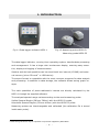
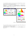
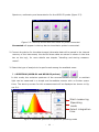
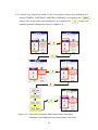
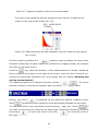
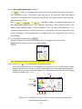
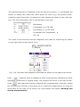
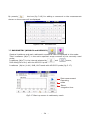
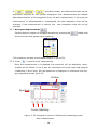
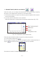
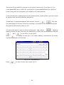
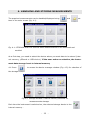
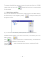
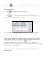
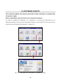
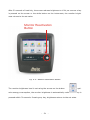
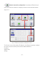
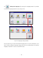
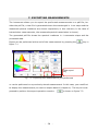
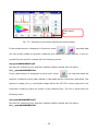
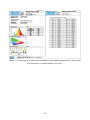
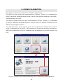
REV. 1.2
01/12/2014
Spectroradiometer - Data Logger
HD30.1
ENGLISH
The quality level of our instruments is the result of the constant development of the
product. This may produce some differences between the information written in this
manual and the instrument you have purchased. We cannot completely exclude the
possibility of errors in the manual, for which we apologize.
Data, images and descriptions included in this manual cannot be legally asserted. We
reserve the right to make changes and corrections with no prior notice.
TABLE OF CONTENTS
1 . INTRODUCTION...................................................................................... 4 2 . INSTRUMENT COMMISSIONING .............................................................. 7 3 . MEASUREMENT GUIDE ...........................................................................10 4 . HANDLING AND STORING MEASUREMENTS ............................................35 5 . SOFTWARE UPDATE ...............................................................................46 6 . INSTRUMENT SETUP ..............................................................................48 7 . EXPORTING MEASUREMENTS .................................................................58 8 . STORAGE...............................................................................................62 9 . PROBE CALIBRATION ............................................................................63 10 . TECHNICAL FEATURES .........................................................................64 11 . ORDERING CODES ...............................................................................67 -
2
-
Spectroradiometer_Data Logger
HD30.1
-
3
-
1. INTRODUCTION
Fig.1.1 Data logger-indicator HD30.1
Fig.1.2 Measuring probe HD30.S1
Measuring probe HD30.S2
The data logger-indicator, running Linux operating system, handles data processing
and management. It has a large color touchscreen display, ensuring easy execution, display and logging of measurements.
Spectra and derived quantities can be saved both into internal (150MB) and external memory (micro SD-card1 or USB device).
The export format is compatible with the most common programs for data analysis
and processing. In addition to data storage, the software allows saving graph images.
The main quantities of photo-radiometric interest are directly calculated by the
HD30.1 through the supplied software.
The analyzed spectral range varies according to the used measuring probe:
Visible Spectral Region (380nm-780nm) with the HD30.S1 probe,
Ultraviolet Spectral Region (220nm-400nm) with the HD30.S2 probe.
Measuring probes are interchangeable and calibrated (the calibration file is stored
inside each probe).
1
Delta Ohm guarantees only for operation on products supplied by Delta Ohm.
-
4
-
The probe HD30.S1 analyzes the visible spectral region (380nm-780nm) and calculates the following photo-colorimetric quantities:
Illuminance [lux], Correlated Color Temperature CCT [K], Trichromatic Coordinates [x,y] (CIE 1931) or [u’,v’](CIE1978), CRI (color rendering index,
R1…R14, Ra) , PAR [µmolphot/sm2] (fig. 1.3)
Figure 1.3
The probe HD30.S2 analyzes the ultraviolet spectral region (220nm-400nm) and
calculates the following radiometric quantities:
UVA Irradiance (W/m2), UVB Irradiance (W/m2) and UVC Irradiance (W/m2)
(figure 1.4).
-
5
-
Figure 1.4
Both sensors have a view of the input equipped with a new generation diffuser
which allows optimizing the response according to the cosine law and not introducing any spectral deformation.
Data concerning the calibration of the probe are stored in non-volatile memory and
are read by the indicator.
-
6
-
2. INSTRUMENT COMMISSIONING
The instrument is delivered with disconnected battery pack inside the battery compartment (figure 2.1).
Figure 2.1: Disconnected battery inside battery compartment.
To connect the battery pack, proceed as follows:
1- Remove the cover of the battery compartment (Figure 2.1)
2- Remove the battery pack from the housing (Figure 2.2)
-
7
-
Figure 2.2: Battery removed from housing.
3- Plug the battery pack connector to the HD30.1 device (figure 2.3).
Connector for
battery
to HD 30.1 device
Figure 2.3: Battery connector on HD 30.1 device
4- Insert the batteries into the battery compartment (figure 2.4).
-
8
-
5- Close the cover.
6- Switch the device on with the on/off switch (figure 2.5).
on/off switch
8-pole M12 male connector
for connecting probe
to instrument
Figure 2.5: On/Off switch.8-pole M12 male connector
for connecting probe to instrument
The instrument works both with the battery and the external power supply (if power
supply is used, the battery must be installed into the instrument).
-
9
-
3. MEASUREMENT GUIDE
1. When switching the instrument on, a yellow led (steady at first and then blinking)
shows that the instrument is starting. After 20 seconds, the instrument is operating
and the start-up screen appears if no probe is connected (fig 3.1)
Figure 3.1: Start-up screen with no probe connected.
all measurement functions in the screen are disabled.
appears in the header (blue bar on the top of the
screen).
If a probe is already connected to the HD30.1 or is connected after the start-up, the
splash screen shows the enabled measurement options available for the connected
probe:
Spectrum, photo-colour, radiometry and transmission for the HD30.S1 probe (figure
3.2),
Figure 3.2: Start-up screen with HD30.S1 probe connected.
-
10
-
Spectrum, radiometry and transmission for the HD30.S2 probe (figure 3.3)
Figure 3.3: Start-up screen with the HD30.S2 probe connected.
Connected will appear in the top bar to show that a probe is connected.
2. Connect the device for the data storage (otherwise data will be saved in the internal
memory of the instrument; the device where data are stored is shown in the blue
bar on the top), for more details see chapter “Handling and storing measurements”.
3. Select the type of analysis to be performed among the available ones:
3.1 SPECTRUM (HD30.S1 and HD30.S2 probes)
,
In this mode, the emission spectrum of the sources can be displayed or ambient
light can be measured in a simple and immediate manner with no further operations. The start-up screen for this measurement will be displayed as shown on figure 3.4.
Start measuring
Operating
mode
Select integration
time
Fig.3.4: Measured spectrum in Spectrum operating mode
-
11
-
3.1.1. Select the operating mode of the instrument among the available four
modes (SINGLE, CONTINUE, MONITOR, LOGGING). By pressing the
button two arrow sliders are displayed; by pressing the
operating mode changes as shown on figure 3.5.
Figure 3.5: Select the operating mode using the arrow keys.
Selection keys disappear by pressing any other key.
-
12
-
button the
3.1.1.1 SINGLE
Single measurement. The measurement is started by pressing
. Once the
measurement is completed, the results are saved in a file with the file name automatically assigned (the name of the saved file is like: spv-yymmddHHMMSS.txt for
measurements performed by the probe HD30.S1 and spu-yymmddHHMMSS.txt for
measurements performed by the probe HD30.S2).
3.1.1.2 CONTINUE
Measurements performed are continuous. Measurements are started by pressing
the
button, once the measurement is completed; the instrument starts a new
measurement. Measurements are stopped by pressing the
button. All meas-
urements are stored in a directory named spv-yymmddHHMMSS.txt for measurements performed with the HD30.S1 probe and spu-yymmddHHMMSS.txt for measurements performed with the HD30.S2 probe.
3.1.1.3 MONITOR
Measurements performed are continuous and are started by pressing
, once
the measurement is completed, the instrument starts a new measurement. Measurements are stopped by pressing
.
Note: Measurements are not saved.
3.1.1.4 LOGGING
The instrument performs a measurement on expiry of a set time interval. The logging interval can be selected among the following time intervals:
3, 5, 10, 15, 30, 60 min.
Logging is enabled by pressing
and stopped with
. All measurements
are saved in a single directory automatically created under the name of LOGyymmddHHMMSS (logging start date and time), files saved in the directory will be
named spv-yymmddHHMMSS.txt for measurements performed with the HD30.S1
and spu-yymmddHHMMSS.txt for measurements performed with the HD30.S2.
While measuring, the page header blinks red and shows the remaining time before
next log.
.
3.1.2 Integration time calculation. Integration time selection is automatic by default. Pressing the
button the two arrows for the manual setting of the in-
tegration time are displayed:
-
13
-
3.1.2.1 Manual Selection: the integration time is manually selected with
arrow keys. The available integration times are: 1, 2, 4, 8, 16, 32, 64, 128,
256, 512, 1024, 2048, 4096 ms.
At the top of the graph, the instrument will show if the performed measurement is
underexposed or overexposed (figure 3.6)
OVEREXPOSED
OK
UNDEREXPOSED
Figure 3.6: correct exposure time is displayed on top of graph.
In Monitor, Continuous and Logging operating modes, measurements will be all
performed with the same integration time set before starting measurements.
3.1.2.2 Automatic Selection (default)
In
mode, at the start of the measurement, the instrument searches for
the best integration time. The search may take up to 30 seconds. Once the search
process is completed, the instrument carries out the measurement by using the
optimal integration time.
-
14
-
If the instrument is in
,
and
operating modes, it will
start searching for the optimal integration. Measurements are started after determining the integration time. At each measurement, if the previous measurement
is underexposed, the new integration time will be increased; if it is overexposed,
the integration time will be reduced, if the measurement is optimal, the new integration time will not be changed.
3.1.3 Averaged Measurements
Set the desired number of samples to be averaged by means of the
key
and of the arrow keys that appear when the key is pressed
(the maximum number of averaged samples is set to 20).
3.1.4 Press the
key to perform the measurement.
Once the measurement is completed, the spectrum will be displayed; wavelengths
will be shown in the X-axis as nanometers (220nm-400nm for the HD30.S2 probe,
380nm-780nm for the HD30.S1 probe) and the measured spectral irradiances in
the Y-axis: the last spectrum is displayed in continuous and logging operating
modes (figure 3.7).
Scroll
cursors
Export
Enter
comment
-
15
-
Figure 3.7: Spectrum display at the end of measurement
The name of the saved file and the integration time used for measuring are
shown on top right of the screen (fig. 3.8)
SPV_140921154215
T=256ms
Figure 3.8: Data concerning file and integration time are shown on top right of
the screen.
Exit the screen by pressing the
key (bottom right) to display the other meas-
urements concerning the same acquisition (continuous or logging mode), the program
will return to the main screen.
Press the
key, select the directory of the measurements of interest, upload the
file by using the arrow keys on the right of the screen, scroll the files of interest concerning the performed acquisition (for more details see the chapter Handling and
storing measurements).
The measured spectrum is displayed with two cursors (
,
). The cursor
position is shown on the top bar together with the measured irradiance value.
Initially, the cursor
while
is positioned on the maximum spectral irradiance value,
is positioned at the extremity of the wavelength available on the probe.
You can select which cursor should be moved using the
key, select
if
you want to move the two cursors at the same time. Cursors are moved by using the
arrow keys
(to move the cursor to the left) ,
the right).
-
16
-
(to move the cursor to
By pressing the
key the box (fig. 3.9) for adding a comment to the measure-
ment shown on the screen will be display.
Fig. 3.9 : Comment Box
Press
to return to the main menu Fig.3.1.
3.2 PHOTO-COLOR (HD30.S1 Probe)
This operating mode is active only with the probe HD30.S1. Besides the emission
spectrum, the main photo-colorimetric quantities can be displayed, such as:
illuminance (Lux), trichromatric coordinates CIE 1931 (x, y) and CIE 1976 (u’,v’), the
Correlated Color Temperature CCT (K) and the Color Rendering Index CRI (the general index and the index of each of the 14 reference samples). By pressing the Photocolor button you access the screen in figure 3.10
Start measuring
Operating
mode
Select integration
time
Figure 3.10: Photo_color measuring mode startup screen
-
17
-
3.2.1 Select the operating mode of the instrument among the four available modes
(SINGLE, CONTINUE, MONITOR, LOGGING). By pressing
cursors are displayed, pressing
the two scroll arrow
makes the operating mode change as shown on
figure 3.11.
Figure 3.11: Select the operating mode using the arrow keys.
Selection arrow keys disappear when pressing any other key.
-
18
-
3.2.1.1 SINGLE
Single measurement. Measurement is started by pressing the
key. Once
the measurement is completed, the results are saved in a file with an automatically
assigned
name
(the
name
of
the
saved
file
is
like:
spv-
yymmddHHMMSS.txt.
3.2.1.2 CONTINUE
Measurements are performed in continuous. Measurements are started by
pressing the
button; once the measurement is completed, the instru-
ment starts a new measurement. Measurements are stopped by pressing
button. All measurements are stored in a work directory named spvyymmddHHMMSS.txt.
3.2.1.3 MONITOR
Measurements are performed continuously and are started by pressing
,
once the measurement is completed, the instrument starts a new measurement. Measurements are stopped by pressing
.
Note: Measurements are not saved.
3.2.1.4 LOGGING
The instrument carries out a measurement on the expiry of a set interval. The
logging interval can be selected among the following time intervals:
3 , 5 , 10 , 15 , 30 , 60 min.
Logging is started by pressing
and stopped by pressing
. All
measurements are saved in a single, automatically created directory named
LOG-yymmddHHMMSS (logging start date and time), files saved in the directory
will be named spv-yymmddHHMMSS.txt. While measuring, the page header
blinks red and shows the remaining time before next log.
.
3.1.2
Integration time calculation selection. Integration time selection is
automatic by default. Pressing the
button displays the two arrows for
the manual setting of the integration time:
-
19
-
3.2.2.1 Manual Selection: the integration time is selected manually by using the
arrow keys
. The available integration times are: 1, 2, 4, 8, 16, 32, 64, 128,
256, 512, 1024, 2048, 4096 ms.
On top of the graph the instrument will show if the measurement just performed is
underexposed or overexposed (figure 3.12).
OVEREXPOSED
OK
UNDEREXPOSED
Figure 3.12: The correct exposure is displayed on top of the graph.
In Monitor, Continuous and Logging operating modes, measurements will be all
carried out with the same integration time set before starting measuring.
-
20
-
3.2.2.2 Automatic Selection (default)
In
mode, at measurement start-up the instrument searches for the opti-
mal integration time. The search may take up to 30 seconds. Once the search
process is completed, the instrument carries out the measurement with the optimal integration time.
With
,
or
operating modes, at measurement start-up
the instrument searches for the optimal integration time. Measurements are
started after determination of the integration time. At each measurement, if the
previous measurement is underexposed or overexposed, the new integration time
will be changed; if the measurement is optimal, the new integration time will not
be changed.
3.2.3 Averaged measurements
Set the number of the desired samples to be averaged by pressing the
button and the arrow keys that appear
(the maximum number of averaged samples is set to 20).
3.2.4 Press the
key to perform the measurement.
Once the measurement is completed, the spectrum will be displayed, wavelengths will be shown in the X axis as nanometers and the measured spectral irradiances in the Y-axis: the last spectrum is displayed in continuous and logging
operating modes (fig. 3.13)
Outline
Spectrum
Color space
x,y CIE1976
CRI
Cursors handling
Figure 3.13: Example of screen in Photo-color measuring mode after
measurement completion.
-
21
-
The acquired spectrum is displayed on the top left of the screen; x, y coordinates are
shown on bottom left, inside the colour space CIE 1932 (x,y); the general colourrendering index Ra and the 14 indexes for each sample are shown on the right bottom. The main photometric info is summarized on top right:
Illuminance
Coordinates (x,y) CIE 1931
Coordinates (u’,v’) CIE 1976
Correlated Color Temperature
K
CRI Ra
The name of the saved file and the integration time used for measuring are shown
on top right of the screen (figure 3.14).
SPV_1409211542150
T=256ms
Fig. 3.14: file name and integration time data are shown on top right of the screen
Press
(bottom right) to display the other measurements related to the same
acquisition (continuous or logging mode), the program will return to the main screen.
Press
and select the directory related to the measurements of interest, upload
the file and scroll the files of the same log or continuous measurement by using the
arrow keys on the right of the screen (for more details see chapter Handling and
storing measurements).
-
22
-
The measured spectrum is displayed together with the two cursors (
,
).
The position of the wavelength the two cursors are pointing to is shown on the top bar
along with the value of the measured spectral irradiance and of the cursors’ wavelength.
At first,
cursor is positioned on the maximum spectral irradiance value, while
is positioned at the extremity of the wavelength available on the probe.
You can select which cursor should be moved using the
button; select
if you want to move the two cursors at the same time. Cursors are moved using the
arrow keys
Press
Press
and
(to the left or to the right).
to return to the main menu Fig.3.1.
(bottom bar) to display one graph at a time following the sequence below
Figure 3.15.
Figure 3.15: Different displays of the measurements acquired in photo-color mode.
Press
to move from one display to next one.
-
23
-
By pressing
the box (fig 3.16) for adding a comment to the measurement
shown on the screen will be displayed.
Figure 3.16 : comment box
3.3 RADIOMETRY (HD30.S1 and HD30.S2)
,
Spectral irradiance and main radiometric quantities can be displayed in this mode:
Total irradiance (W/m2) in the entire spectral range covered by the currently used
probe,
Irradiance (W/m2) in the interval selected by
and
cursors,
PAR uMol/(fot*s*m2) with the HD30.S1 probe
Irradiance (W/m2) in UV, UVB, UVC bands with HD30.S2 probe (fig 3.17).
Start measurement
Operating
mode
Select
Integration time
Fig3.17 Start-up screen in radiometry mode
-
24
-
3.3.1 Select the operating mode of the instrument among the four available modes
(SINGLE, CONTINUE, MONITOR, LOGGING). Press
sors, press
Fig 3.18:
to display two scroll cur-
to change the operating mode as shown on figure 3.18.
Select the operating mode using the arrow keys.
Selection arrow keys disappear when pressing any other key.
-
25
-
3.3.1.1 SINGLE
Single measurement. Measurement is started by pressing
. Once the
measurement is completed, results are saved in a file with an automatically assigned file name (the name of the saved file is like: spv-yymmddHHMMSS.txt
for
measurements
performed
with
the
HD30.S1
probe
and
spu-
yymmddHHMMSS.txt for measurements performed with the HD30.S2 probe).
3.3.1.2 CONTINUE
Measurements are carried out in continuous mode. Measurements are started
by pressing the
key; once the measurement is completed, the instrument
starts a new measurement. Measurements are stopped by pressing
. All
measurements are saved in the work directory named spv-yymmddHHMMSS.txt
for measurements performed with the HD30.S2 probe.
3.3.1.3 MONITOR
Measurements are carried out in continuous mode and are started by pressing
; ; once the measurement is completed, the instrument starts a new measurement. Measurements are stopped by pressing
.
Note: measurements are not saved.
3.3.1.4 LOGGING
The instrument performs a measurement on expiry of a set time interval. The
logging interval can be selected among the following time intervals:
3, 5, 10, 15, 30, 60 min.
Logging is enabled by pressing
and stopped with
. All measure-
ments are saved in a single directory automatically created under the name of
LOG-yymmddHHMMSS (logging start date and time); the files saved in the directory will be named spv-yymmddHHMMSS.txt for measurements performed
with HD30.S1 and spu-yymmddHHMMSS.txt for measurements performed with
HD30.S2. While measuring, the page header blinks red and shows the remaining time before next log.
.
3.3.2 Integration time calculation selection. The integration time is automatically selected by default. Press
to display the two arrows for the man-
ual setting of the integration time:
-
26
-
3.3.2.1 Manual Selection: the integration time can be manually selected by using
The available integration times are: 1, 2, 4, 8, 16, 32, 64, 128, 256, 512, 1024,
2048, 4096 ms.
The instrument will show on top of the graph if the measurement just performed
is underexposed or overexposed (fig 3.19)
OVEREXPOSED
OK
UNDEREXPOSED
Fig 3.19: Correct exposure is displayed on top of the graph.
In Monitor, Continuous and Logging operating modes, measurements will be all
carried out with the same integration time set before starting measuring.
3.3.2.2 Automatic Selection (default)
In
mode, at measurement start-up the instrument searches for the op-
timal integration time. The search may take up to 30 seconds. Once the search
process is completed, the instrument carries out the measurement with the optimal integration time.
-
27
-
In
,
o
r operating modes, at measurement start-up the
instrument searches for the optimal integration time. Measurements are started
after determination of the integration time. At each measurement, if the previous
measurement is underexposed or overexposed, the new integration time will be
changed, if the measurement is optimal, the
new integration time will not be
changed.
3.3.3 Averaged measurements
Set the desired number of averaged samples by pressing the
button and
the arrow keys that appear when pressing
(The maximum number of averaged samples is set to 20).
3.3.4 Press
to perform the measurement.
Once the measurement is completed, the spectrum will be displayed; wavelengths will be shown in the X-axis as nanometers and the measured spectral
irradiances in the Y-axis: the last spectrum is displayed in continuous and logging operating modes (fig 3.20)
Outline
Spectrum
Cursor Handling
Figure. 3.20: Example of screen in Radiometry measuring mode
after measurement.
-
28
-
Irradiance integral values are shown on top of the screen :
Irradiance between the two cursors L1_L2;
Total Irradiance
PAR (only with HD30.S1 probe)
UV Irradiance (only with HD30.S2 probe)
UVB Irradiance (only with HD30.S2 probe)
UVC Irradiance (only with HD30.S2 probe)
The name of the saved file and the integration time used for measuring are displayed
on top right of the screen (fig. 3.21)
SPV_141112150012
T=64ms
Fig. 3.21: File name and integration time data are shown on top right of the screen
Press
(bottom right) to exit and display the other measurements concerning
the same acquisition (continuous or logging mode), the program will return to the
main screen. Press
to select the directory with the desired measurements,
upload the file and scroll the files related to the same log or continuous measurement
-
29
-
using the arrow keys on the right of the screen (see chapter Handling and storing
measurements for more details).
The measured spectrum is displayed together with the two cursors (
,
).
The position of the wavelength indicated by the two cursors is shown in the top bar
along with the measured spectral irradiance value and the wavelength of the cursors.
At first
cursor is positioned
on the maximum spectral irradiance while
is positioned at the extremity of the wavelength available on the probe.
Press the
button and select the cursor you want to move; select
move the two cursors at the same time. Cursors are moved by using
to
and
arrow keys (to the left or to the right).
By pressing
the box (fig. 3.22) where you can add a comment to the measure-
ment shown on the screen will be displayed.
Fig 3.22 : Comment box
Press
to return to the main menu Fig.3.1.
-
30
-
3.4 TRANSMITTANCE (HD30.S1 and HD30.S2)
,
.
Under this mode, you can measure the transmission in the spectral range covered by
the probe in use. Measurement is carried out in two distinct steps;
A- the first step needed is to acquire the reference spectrum (against which transmission will be calculated) ,
B- only later spectral transmission can be measured.
Select the transmission of measurement to access the window below (Fig. 3.23):
Start measurement
Reference
Select
Integration time
Fig. 3.23: Transmission measurement screen
Follow the steps indicated hereafter to acquire the reference spectrum:
3.4.1 Set average measurement
Set the number of samples you wish to be averaged to perform measurements by using the
key and the arrows that appear when the key is pressed.
(the maximum number of averaged samples is set to 20).
-
31
-
3.4.2 Integration Time calculation. The integration time selection is automatically
made by default through the dedicated button; use the arrows to perform the desired
selection:
3.4.2.1 Manual selection: the integration time is manually selected using the arrows
: 1, 2, 4, 8, 16, 32, 64, 128, 256, 512, 1024, 2048, 4096 ms.
The instrument will show in the upper end of the spectrum if the spectrum reference
measurement just performed is underexposed or overexposed (fig. 3.24)
OVEREXPOSED
OK
UNDEREXPOSED
Fig. 3.24: The correct exposure is indicated on top of the graph.
3.4.2.2 Automatic selection (default)
The instrument searches for the optimal integration time when the reference measurement is started. The search can take up to 30 seconds. At the end of the search,
the instrument performs the measurement with the optimal integration time.
-
32
-
The integration time used for the calculation of the reference spectrum will be kept for
all transmission of the measurements.
3.4.3
Press REF to acquire the reference spectrum. The spectrum is displayed on
the screen (fig. 3.25).
Fig. 3.25 : Reference spectrum acquisition
At this stage the
button is enabled and the transmission measurement can be
carried out.
3.4.4 By pressing the Start button (enabled only if the reference spectrum has been
performed) you launch the transmission measurement displayed on the screen Fig.
(3.26),
Fig. 3.26: Spectral transmission measurement.
-
33
-
The name of the saved file is shown on top right of the screen (in the form of trvyymmddHHMMSS.txt for HD30.S1 probe and tru-yymmddHHMMSS.txt for HD30.S2
probe) along with the integration time used for the measurement.
A new transmission measurement can be performed by pressing Start (you don’t need
to acquire each time the reference spectrum).
Transmission is displayed together with the two cursors (
,
). The posi-
tion wavelength of the two cursors are pointing to is shown on the top bar along with
the spectral transmission value (in %).
You can select which cursor to move by using the
button,
selecting
buttons moves the two cursors at the same time. Cursors can be moved by using the
arrows
Press
and
(to the left or to the right).
to display the box (fig. 3.27) where adding a comment to the meas-
urement displayed on the screen.
Fig. 3.22 : Comment box
Press
to return to the main menu Fig.3.7.
-
34
-
4. HANDLING AND STORING MEASUREMENTS
The acquired measurements can be handled/displayed using
and
but-
tons in the main screen (fig. 4.1)
Fig. 4.1: STORAGE and FILE buttons allow measurements to be monitored and
recalled.
As a first step, you need to select the device where you want data to be stored (internal memory, μSDcard or USB device). If the user make no selection, the instrument data storage is set to internal memory
4.1 Press
to access the device manager window (Fig. 4.2) for selection of
the storage device
Fig 4.2: Storage window. Internal memory selected for
measurements storage.
Each time the instrument is switched on, the selected storage device is the
internal memory .
-
35
-
The amount of available free memory is shown at the centre top of the icon (150MB),
a green check mark on top left
indicates that the device is currently selected
for data storage.
4.1.1 Work directory selection.
Once you have selected the internal memory, data are saved in the DATA directory;
the work directory can be changed by pressing
. Pressing the button opens
the figure 4.3 screen.
Fig. 4.3: Screen for work directory creation/selection in the internal memory.
Available directories appear in the centre of the screen, a new directory can be created by pressing
Press
.
to store measurements in a selected directory; the selected work-
ing directory will be displayed in the blue top bar.
Press the
button to erase the internal memory, a window will be dis-
played (Fig. 4.4).
-
36
-
Fig. 4.4: Memory delation dialog box .
Press
to erase the memory. Note: CONFIRMATION OF MEMORY DELE-
TION WILL MAKE DATA RECOVERY IMPOSSIBLE.
4.2 Press
to select μSDcard as default memory. If the card is not present,
the message μSDcard NOT PRESENT will appear. If the memory card is properly installed, the screen will appear as in Fig. 4.5,
Fig. 4.5: Storage screen after selection of the μSDcard
as working memory.
A green check mark will appear on the button
.
4.2.1 Working directory selection
Once you have selected the μSDCard, data are saved in the DATA directory; the working directory can be changed by pressing
. Pressing the button opens the fig.
4.6 screen.
-
37
-
Fig. 4.6: Screen for working directory creation/selection on μSDCARD.
Created directories appear in the centre of the screen; a new directory can be created
by pressing
Press
.
to set measurements storage in a selected directory; the selected
working directory will be displayed in the blue top bar.
To erase the μSDCARD memory, press the
button, a window will be displayed
(Fig. 4.7).
Fig. 4.7: Memory erasure dialog box .
Press
to erase the memory. Note CONFIRMATION OF MEMORY DELA-
TION WILL MAKE DATA RECOVERY IMPOSSIBLE.
4.2.2 Press
if you want to transfer the content of the HD30.1 internal mem-
ory to the μSDCARD. All data are transferred to the DATA directory; existing data on
the memory card will be overwritten.
-
38
-
4.2.3 Press
if you want to transfer the content of the USB device to the
μSDCARD. All data are transferred to the DATA directory; the existing data will be
overwritten.
4.3 Press
to select the USB device as default storage memory. If the USB de-
vice is not present, the message USB NOT PRESENT will appear. If the device is properly installed, the screen will appear as in Fig. 4.8,
Fig. 4.8: Storage screen after selection of the USB device as working memory
A green check mark will appear on the
button.
4.3.1 Working directory selection
Once you have selected the USB device, data are saved in the DATA directory; the
working directory can be changed by pressing
the fig. 4.9 screen.
-
39
-
. Pressing the button opens
Fig. 4.9: Screen for the creation/selection of the work directory on a USB device.
Available directories appear in the center of the screen, a new directory can be created by pressing
Press
.
to save measurements in a selected directory; the selected work di-
rectory will appear in the blue top bar.
Press
to erase the USB device memory, a dialog box will appear (Fig. 4.10).
Fig. 4.10: Memory erasure dialog box
Press
to erase the memory. Note. CONFIRMATION OF MEMORY DELA-
TION WILL MAKE DATA RECOVERY IMPOSSIBLE.
4.3.2 Press
if you want to transfer the content of the HD30.1 internal mem-
ory to the USB device. All data are transferred to the DATA directory; the existing
data will be overwritten.
-
40
-
4.3.3 Press
if you want the content of the μSDCARD to be transferred to the
USB device. All data are transferred to the DATA directory; existing data on USB device will be overwritten.
4.4 Press
4.5 Press
to return to the main screen (Fig. 4.1).
in the main screen to display stored measurements ( fig. 4.1).
Pressing the button will open the fig. 4.11 window.
Fig. 4.11: display of the measurements stored in one of the available memories (internal memory, µSDcard, USB device).
The screen shows the list of files and directories.
The current memory appears at the bottom of the screen (in the example, the internal
memory has been selected) with a green check mark. You can select another memory
device by pressing one of the available selection
buttons.
A comment can be added into the stored files. This is shown in the comment box.
Select the desired directory to display files; the select the file to be displayed. Press
to return to the selected storage device.
4.5.1 Select the desired file. The selected file will appear on BLUE background (fig.
4.11); at this stage, the file can be displayed using the buttons on the right of the
screen (fig. 4.12).
-
41
-
Fig. 4.12: Data contained into selected file can be displayed by using the highlighted
keys.
Press
to display the selected measurement (Fig. 4.13)
Fig. 4.13: Screen showing SPC_140921165803 file loaded from internal memory with
photo-color analysis.
The arrows highlighted in figure 4.14 allow next measurement to be displayed directly
with no need to go back to the FILE menu (fig. 4.11).
Fig. 4.14 : Arrow keys can be used to display files stored in memory.
-
42
-
The spectrum is displayed together with the two cursors (
,
). The po-
sition of the wavelength the two cursors are pointing to is shown on the top bar along
with the measured spectral irradiance value and the wavelength of cursors.
cursor is positioned on the maximum spectral irradiance while
is posi-
tioned on the bigger wavelength available on the current probe.
Pressing
allows you to select the cursor you want to move, selecting
will allow you to move the two cursors at the same time. Cursors are moved using the
arrow keys
towards the left or the right.
Pressing
allows you to add a comment to the measurement performed.
Press
to return to the FILE menu (Fig.4.11).
Press
(bottom bar) to display one graph at a time following the sequence be-
low Fig. 4.15.
Fig.4.15: Various displays in photo-colour mode. Press
to the next one.
-
43
-
to move from a display
Press
to display the box (fig. 4.16) where a comment can be added to the
measurement shown on the screen.
Fig. 4.16 : Comment box.
4.6 Press
to display (fig. 4.17) the spectral irradiance data in steps of 1 nm,
Fig. 4.17: Spectral irradiance data in text format
-
44
-
Press
to return to the previous page.
Press
to
4.7 Press
return to the file handling page (fig. 4.11)
in the file handling window to return to the start-up screen (fig.
4.18)
Fig. 4.18: Returning to the main menu from stored measurements management
menu
-
45
-
5. SOFTWARE UPDATE
The software update can only be performed if the instrument is powered by
the power supply.
Before upgrading, save the data into an external memory.
In order to update the software, it is necessary to connect the instrument to an
Ethernet network. Once you the instrument has been connected from the main menu,
press the keys following the sequence in figure 5.1,
Fig. 5.1: Sequence to be followed for software update.
-
46
-
The last screen of figure 5.1 shows the currently used software version; press
to connect the instrument to DeltaOhm web site and check the update
status of the software under usage.
If a more updated software version is available, the program asks for the permission
of updating the software - Figure 5.2:
Fig. 5.2: Confirmation window for software update.
Once the software update has been allowed, the new version is downloaded and installed.
The new software becomes operational the next time the instrument is turned on.
If for any reason the instrument cannot be connected to the network, a message appears.
-
47
-
6. INSTRUMENT SETUP
Press
press
in the main menu to access the HD30.1 configuration page (fig. 6.1),
to exit the SETUP menu.
Fig. 6.1: HD30.1 configuration page
The SETUP menu includes 8 buttons with the following functions:
-
48
-
6.1
Activating acoustic signals. When the program starts, the Buzzer is ac-
tive and each press of a button is indicated by a sound; in order to disable this function, it is necessary to press the BUZZER key, so to change its status (Figure 6.2).
Fig. 6.2: Activating/deactivating acoustic signals through Buzzer key.
-
49
-
6.2
Power saving configuration. Press the POWER SAVING button to ac-
cess the window for the management of the brightness level of the screen and the
Stand-by time Figure 6.3,
Fig. 6.3 Power Saving Management Window
By using the arrows on the button
it is possible to set the time interval after
which the screen is turned off (if no key is pressed). In order to activate the screen
again, it is necessary to press the white button on the HD30.1 (Figure 6.4).
-
50
-
After 30 seconds of inactivity, the screen reduces brightness to 10%; as soon as a key
is pressed on the screen or the white button on the instrument, the monitor brightness returns to the set value.
Monitor Reactivation
Button
Fig. 6.4 : Monitor reactivation button
The monitor brightness level is set using the arrows on the button
. To opti-
mize energy consumption, the monitor brightness is automatically reduced if no key is
pressed within 30 seconds. Pressing any key, brightness returns to the set value.
-
51
-
Pressing
will change the status and the following icon will appear
. In
this way, the ON/OFF and power saving functions of the monitor screen are disabled.
The charge level of the batteries is shown on the starting page in the blue band at the
top right (Figure 6.5).
Battery Level
Fig. 6.5: Battery level
Next to the charge level is shown the presence of the power supply (Figure 6.6)
Power supply indication
Fig. 6.6: Indication of power supply
When the charge level of the batteries reaches 10%, a message appears on the
screen prompting the user. With the battery charge below 10% the instrument does
not perform any measurements.
-
52
-
6.3
Network connection configuration. By pressing the Ethernet key al-
lows you to access the window for managing connection to the instrument network
(Figure 6.7).
Fig. 6.7 Ethernet connection configuration menu.
The first box on top of the window (IP address) in the Ethernet connection configuration menu concerns the setting of the network address defined by:
IP address
SUBnet mask
GATway
-
53
-
Pressing
changes from DHCP mode to manual mode. In the first case, it is the
router that assigns the IP address to the device (default setting). In the second case,
parameters for connection must be defined by the user.
The second box at the bottom of the window is used to define primary and secondary
DNS.
Note: The connection to the network is necessary for the software update.
-
54
-
6.4
Setting the Language. By pressing the Language button it is possible
to access the language selection menu (Figure 6.8)
Fig. 6.8: Language setting window
On top right of the icon with the selected language there is a green checkmark; if you
wish to select a different language, simply press the key corresponding to the desired
language. Press EXIT to return to the SETUP menu.
-
55
-
6.5
Setting date and time. By pressing the Date-time button it is possible
to access the window for date/time setting (figure 6.9).
Fig. 6.9: Date/Time setting window
Once you have properly set date and time, use the arrow keys to press
make the change effective.
Press
to return to the SETUP menu.
-
56
-
and
6.6
6.7
HELP. Pressing Help allows you to refer to the user manual.
Checking and updating the Software. See chapter 5 for a detailed ex-
planation of the About key.
6.8
EXIT. Pressing Exit makes you return to main menu (Fig. 6.1)
-
57
-
7. EXPORTING MEASUREMENTS
The instrument allows you to export the performed measurements to a pdf file; besides the pdf file, a text file is generated where the wavelength in 1-nm steps and the
measured spectral irradiance are shown respectively in two columns (in the case of
transmission measurements, the measured spectral transmission is shown).
The generated pdf file shows the spectral irradiance in 1 nanometer steps and the
processed data.
Export can be performed at the end of the measurement by pressing the
key in
figure 7.1
Data export
key
Fig. 7.1: Exporting the measurement just performed
or can be performed on a previously stored measurement. In this case, you need first
to display the measurement you want to export data of (chapter 4). The key to be depressed to perform the export operation remains
-
58
-
as shown on figure 7.2.
Data export
key
Fig. 7.2: Exporting a previously performed measurement
If the measurement is displayed in Spectrum mode
,
exported data
are only those related to spectral irradiance (the spectrum image appears in the exported file) and the file is saved with the following name:
rsp-yymmddHHMMSS.pdf
the text file containing only spectral irradiance data is saved with the name :
r1n_ yymmddHHMMSS.txt
If the measurement is displayed in photo-color mode
the exported data are
spectral irradiance and all data related to calculated photo-colorimetric quantities (the
spectrum image, the x,y coordinates image within the CIE 1931 colour space and the
chromatic rendering index are shown in the exported file). The file is saved with the
following name:
rph-yymmddHHMMSS.pdf
the text file containing only spectral irradiance data is saved with the name:
r1n_ yymmddHHMMSS.txt
-
59
-
If the measurement is displayed in radiometry mode
,
the exported
data are spectral irradiance and all the calculated radiometric data (the spectrum image appears in the exported file). The file is saved with the following name:
rrd-yymmddHHMMSS.pdf
the text file containing only spectral irradiance data is saved with the name:
r1n-yymmddHHMMSS.txt
In transmission measurements
,
, spectral transmission is exported in
1 nanometer steps , (the spectral transmission image appears in the exported file) :
rtr-yymmddHHMMSS.pdf
the text file containing only spectral irradiance data is saved with the name:
r1n-yymmddHHMMSS.txt
Figure 7.3 shows an example of a report generated in photo-color mode. Is possible to
change the
with other immages .
To change image , save the image to insert as "logo.png" on microSDcard, in main
directory, at this point every time the report is generated the image will appear in
place of the written logo. To have no deformation of the inserted image aspect ratio of
width to height should be 2.4.
-
60
-
Figure 7.3: Example of a report of the measures generated automatically. Space with
the word logo is customizable by the user.
-
61
-
8. STORAGE
Storage conditions for the instrument:
• Temperature: -25...+70°C.
• Humidity: 10...90%RH non condensing
• Avoid storage in areas with:
High humidity levels
Strong electromagnetic fields
The instrument is exposed to direct solar radiation
The instrument is exposed to a high temperature source
Presence of strong vibrations
Presence of vapour, salt and/or corrosive gases
The instrument enclosure is made of ABS plastic: do not use solvents not compatible
for cleaning purposes.
-
62
-
9. PROBE CALIBRATION
Each probe is individually calibrated in DeltaOhm laboratories.
The HD30.S1 probe covers the visible spectrum (380nm -780nm); it is calibrated by
using a reference standard halogen lamp of which the spectral irradiance at the different wavelengths is known.
The HD30.S2 probe covers the ultra-violet spectrum (220nm -400nm); it is calibrated
by using a reference standard deuterium lamp of which the spectral irradiance at the
different wavelengths is known.
The calibration file is stored into the probe and is read by the software each time the
probe is connected to the HD30.1. By pressing the Probe set up button the data related to the calibration file of the installed probe is displayed in the main window (Fig.
8.1):
Fig. 8.1: Access to the window displaying info on connected probe calibration
-
63
-
10. TECHNICAL FEATURES
MODEL
Sensor
Spectral Range
Type of Spectrometer
Numerical Aperture
Input Slit
Pass band
Wavelength Accuracy
Wavelength reproducibility
Integration Time
Integration Mode
Stray Light
Measuring Mode
Measurement typology
HD30.1 +HD30.S1
HD30.1 + HD30.S2
Linear CCD (2048 elements)
Linear CCD (2048 elements)
380 nm – 780 nm
220 nm – 400 nm
Based on transmission diffraction grating
0.16
125µm
70µm
4.5nm
2.5 nm
0.3 nm
0.1 nm
1ms to 4 s
Automatic/manual
<0.03%
<0.03%
Spectral Irradiance, Irradiance,
Illuminance [lux], PAR , Proximal
Spectral Irradiance, UV IrradiColor Temperature, CIE 1931
ance, UVB Irradiance, UVC Irradi(x,y) & CIE 1976 (u’,v’) Trichroance, Spectral Transmittance
matric Coordinates ,CRI, Spectral
Transmittance
Single, single acquisition with data storage
Continuous, continuous acquisition with data storage
Monitor, continuous acquisition without data storage
Logging, acquisition at set time intervals
(3min to 60min) with data storage
Input Optics Dimensions
(quartz diffuser)
Φ 11.8 mm
Cosine Correction
Opaline quartz diffuser (3mm)
Calibration
Range of use
Halogen Lamp
Illuminance 5-70.000 lux
Spectral Irradiance
+- 5 %
Illuminance
+-4%
PAR
+-4%
CCT
+- 45K
x,y
+- 0.002
CRI
+- 1.5
Incertitude
Operating system
Display
Data Storage
PC Connection
Power Supply
Exported Data Format
HD30.1
Dimensions/Weight
Probe
Dimensions/Weight
Working Temperature
Update
Opaline quartz diffuser (2mm)
Deuterium Lamp
Spectral Irradiance
UV Irradiance
UVB Irradiance
UVC Irradiance
+- 15 %
+-6%
+-8%
+-10%
Linux
4.3” touch screen (480x272 pixel)
Internal (150 MB) , micro SD card, USB device (option)
Through Ethernet cable, through mini USB connector.
3.7V 6600 mA/h Li-po rechargeable battery or external power supply
SWD06 (6Vdc-1.5A)
Compatible with the more well-known data management/analysis software
135x 156 x H 42 mm
440 g
75x150x H74, cable length 1.5m
370 g
0°C-40°C
automatic via Internet
-
64
-
The HD30.1 is connected to HD30.S1 or HD30.S2 probes through a cable; use a 8pole male M12 connector to connect the probe to the instrument (fig. 10.1) located
next to the ON/OFF switch.
on/off switch
8-pole M12 male connector
for connecting probe
to instrument
Fig. 10.1: Connector for probe connection to instrument.
The instrument is equipped with ports for connection to the network and for the use of
memory devices (µSDCARD and USB devices) shown in figure 10.2 and figure 10.3.
An unused connector appears in the same figure (10.2).
μSDCARD
USB HOST
Figure 10.2: Connectors for µSDCARD and USB HOST.
-
65
-
Ethernet
Battery charger
Power supply
USB DEVICE
Figure 10.3: USB DEVICE, Ethernet port and power supply/battery charger connectors.
-
66
-
11. ORDERING CODES
HD30.1 + HD30.S1 probe
KIT
including:
Data
logger-Indicator
HD30.1,
HD30.S1 for measurements in the visible spectrum
(380nm-780nm), 4GB micro SDcard, power supply/ battery charger SWD06, case and CD with
manual and software.
HD30.S2
HD30.S2 probe for measurements in the ultraviolet
spectrum (220nm-400nm).
ACCESORIES
SWD06
Power supply/ battery charger for HD30.1
BAT 30
3.7V 6600mA spare battery for HD30.1.
microSD
4GB Micro SD card
HD30S
Additional copy of Software for HD30.1
VTRAP30
Tripod to be fastened to the instrument height
280mm
-
67
-