Download Antelope Toolbox for Matlab: Version 1.1 User`s Manual and Tutorial

Antelope Toolbox for Matlab:
Version 1.1
User’s Manual and Tutorial
Kent Lindquist
Lindquist Consulting, Inc.
updated Aug 21, 2009
Introduction
This document describes an Antelope Software toolbox for Matlab. Matlab is a product of Mathworks, Inc.
Antelope is a product of Boulder Real-Time technologies, Inc. Included in Antelope is the Datascope relational
database system. The major strengths of this Matlab toolbox include those of the Antelope package itself, such
as schema-independent relational database support, a generalized and powerful parameter-file management
architecture, and a number of tools useful to seismologists.
This toolbox follows closely the interfaces to Datascope and Antelope built into other scripting environments
such as Perl and TCL/Tk. This toolbox was developed under Solaris 2.6 on Sun Ultra computers, using Matlab
version 5.3, and has since been upgraded for consistency with Solaris 2.8, Linux, and Matlab 6.5.
Installation
The source code for the Antelope Toolbox for Matlab is available via the Antelope contributed-code web site,
http://www.antelopeusersgroup.org. Successful compilation will place the Antelope Toolbox for Matlab in
$ANTELOPE/data/matlab/<release>/antelope
where <release> indicates the Matlab software release, e.g. “2009a”. For the Antelope Toolbox for Matlab
to compile correctly, the local MATLAB variable must be correctly set with the localmake_config(1)
command. For further details, see the documentation for localmake_config(1). Once the compilation has
been configured correctly with localmake_config(1), the easiest way to compile the toolbox is by running the
program localmake(1) and invoking the antelope_matlab button. Note: Make sure you do not have a conflicting
MATLAB variable (i.e. one pointing to a different version of Matlab) set in your environment during the
compilation process.
After compilation, the paths to the Matlab commands need to be made available to the users. The standard way
to do this is to run the Matlab command
>> run([getenv(‘ANTELOPE’),’/setup.m’])
Each user can execute this by default upon Matlab startup by modifying their own startup.m Matlab file (see
the Matlab documentation for further information on this). Alternatively, the Antelope Toolbox for Matlab can
be made available by default for all users by adding the above command to $MATLAB/toolbox/local/startup.m.
Again, see the Matlab documentation for further details.
Help
All toolbox commands are documented with the standard Matlab help utilities. To see a list of available
commands, type
>> help antelope
or (for the Matlab help window)
>> helpwin antelope
or (for an HTML index of the help entries in a web browser)
>> doc antelope
For a list of examples, type
>> help antelope/examples
‘For help on individual commands, give the name of the command. For example:
>> help dbopen
DBOPEN Open a Datascope Database
DBPTR = DBOPEN ( FILENAME, OPENTYPE )
dbopen opens the database specified by the path name
FILENAME, using the permissions given by opentype. A
database pointer with the database index filled in is
returned in DBPTR. The opentype may be either r (for read
only) or r+ (for reading and writing). In the latter
case, the db package will attempt to open tables
read/write, but if permissions are incorrect, will open
the table read only.
Antelope Toolbox for Matlab
[Antelope is a product of Boulder Real Time Technologies, Inc.]
Kent Lindquist
Lindquist Consulting
1997-2003
>>
The other versions of the help system also work for individual commands:
>> helpwin dbopen
or
>> doc dbopen
For further insight, consult the man pages and manuals provided with the Antelope software and the Matlab
software.
Finally, all commands in the Antelope Toolbox for Matlab come with an example demonstrating their use. To
see the example in action, precede the command with the prefix “dbexample_”. For example, to see the dbopen
command being used, type dbexample_dbopen. There is also a script dbexample_runall which will run all
available examples. This is useful primarily for system testing. There are also a couple example scripts covering
special topics, such as dbexample_joins, dbexample_get_hypocenter_vitals, dbexample_sort_and_subset,
and dbexample_writing.
Opening a Database
Databases are opened with the dbopen command, which takes a filename and a permissions flag. For
convenience the Matlab Antelope Toolbox contains a demonstration database from the Joint Seismic Program
Center. The schema for this database is CSS3.0. The filename of this database is available through the command
>> dbexample_get_demodb_path
demodb_path is /opt/antelope/4.2u/data/matlab/antelope/examples/demodb/demo
>>
The dbopen command returns a four-element structure called a database pointer:
>> db = dbopen(demodb_path,’r’)
db =
database: 0
table: -501
field: -501
record: -501
>>
Under normal conditions the user does not modify these fields directly, with the possible exception of the record
field. Two tools are provided to aim the database pointer at specific parts of the database (i.e. set the integers
correctly). dblookup is the most general of the two. A shorthand version of dblookup, dblookup_table, is
provided for the most common operation, aiming the database pointer at a given table of the database:
>> db=dblookup_table(db,’origin’)
db =
database: 0
table: 10
field: -501
record: -501
>>
Databases may be closed with the dbclose command, which destroys the database pointer:
>> dbclose(db)
>>
Handling Parametric Data
The following examples show some common database operations. These examples presume you have already
opened the database and looked up the origin table, as shown in the steps above. We can subset our database:
>>db=dbsubset(db,’mb > 6’);
Find out how many records we have:
>> dbquery(db,’dbRECORD_COUNT’)
ans =
18
>>
Ask for a column of values:
>> mb=dbgetv(db,’mb’)
mb =
6.4200
6.4000
6.2000
6.2000
6.2300
6.4000
6.3100
6.0200
6.2800
6.5000
6.5700
6.1100
6.0500
6.2100
6.3000
6.3000
6.2700
6.1400
Or ask for several columns of values:
>> [lat,lon,depth,time] = dbgetv(db,’lat’,’lon’,’depth’,’time’);
Convert the epoch-times (seconds since 1970) for the hypocentral occurrence time to a standard readable
format:
>> strydtime(time)
ans =
’ 5/04/1992 (125) 8:45:10.089’
’ 5/12/1992 (133) 18:05:42.600’
’ 5/15/1992 (136) 7:05:05.300’
’ 5/17/1992 (138) 9:49:19.100’
’ 5/17/1992 (138) 9:49:21.689’
’ 5/17/1992 (138) 10:15:31.300’
’ 5/17/1992 (138) 21:36:00.492’
’ 5/19/1992 (140) 14:42:48.813’
’ 5/20/1992 (141) 12:20:34.700’
’ 5/21/1992 (142) 4:59:57.500’
’ 5/21/1992 (142) 5:00:00.399’
’ 5/21/1992 (142) 18:05:48.543’
’ 5/22/1992 (143) 21:40:36.691’
’ 5/25/1992 (146) 2:51:32.311’
’ 5/25/1992 (146) 16:55:04.100’
’ 5/27/1992 (148) 5:13:38.800’
’ 5/27/1992 (148) 5:13:41.635’
’ 5/28/1992 (149) 21:24:51.822’
Or we can customize the time-conversion format:
>> epoch2str(time,’%A %b %d %I:%M %p %Z’)
ans =
’Monday May 04 08:45 AM UTC’
’Tuesday May 12 06:05 PM UTC’
’Friday May 15 07:05 AM UTC’
’Sunday May 17 09:49 AM UTC’
’Sunday May 17 09:49 AM UTC’
’Sunday May 17 10:15 AM UTC’
’Sunday May 17 09:36 PM UTC’
’Tuesday May 19 02:42 PM UTC’
’Wednesday May 20 12:20 PM UTC’
’Thursday May 21 04:59 AM UTC’
’Thursday May 21 05:00 AM UTC’
’Thursday May 21 06:05 PM UTC’
’Friday May 22 09:40 PM UTC’
’Monday May 25 02:51 AM UTC’
’Monday May 25 04:55 PM UTC’
’Wednesday May 27 05:13 AM UTC’
’Wednesday May 27 05:13 AM UTC’
’Thursday May 28 09:24 PM UTC’
>>
As an aside, we can go the other way too:
>> str2epoch(’2/13/98 15:17’)
ans =
887383020
>>
or
>> str2epoch(’now’)
ans =
9.2039e+08
>>
We can pick out the first record in our database view (note the indexing convention!):
>> db.record=0
db =
database: 0
table: 36
field: -501
record: 0
>>
Find the iasp91 P-phase travel time in seconds from the hypocenter to Fairbanks:
>> dbeval(db,’pphasetime(distance(lat,lon,64.836,-147.7048),depth)’)
ans =
780.7877
>>
We can launch a spreadsheet tool (dbe) on our whole database:
>> unix([’dbe ’ demodb_path ’&’])
[1] 17990
ans =
0
>>
and examine the individual tables by clicking on the buttons.
Handling Waveform Data
The database contains data for one earthquake. We can get the data for the P wave in one of two ways. First we
need to get the correct database pointer:
>> db=dblookup_table(db,’wfdisc’);
>> dbt=dblookup_table(db,’arrival’);
>> db=dbjoin(dbt,db);
>> db= dbsubset(db,’arrival.chan == wfdisc.chan’);
>> dbt=dblookup_table(db,’assoc’);
>> db=dbjoin(dbt,db);
>>dbt=dblookup_table(db,’origin’);
>> db=dbjoin(dbt,db);
>> db=dbsubset(db,’sta == “CHM” && chan == “BHZ”’);
>> [time,endtime]=dbgetv(db,’time’,’endtime’)
time =
7.061397100070000e+08
endtime =
7.061398415000000e+08
>>
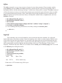
Now we have a couple options for getting data. We can use trload_css to load the database waveform contents
into a trace-object, another database pointer that includes information on waveforms loaded into memory; or we
can use trgetwf. The former, which is the preferred method, requires us to call trextract_data to get the actual
waveform data. Further detail on these commands is provided in their descriptions below, especially in the text
for the trload_css command.
>> tr=trload_css(db,time,endtime);
>>data1=trextract_data(tr);
Or we can go directly to the waveform data from the database pointer:
>> [data2,nsamp,t0,t1]=trgetwf(db,time,endtime);
Response information
Response information stored in a database may be loaded into a dbresponse object for evaluation. We precede
our demonstration of this with an extraction of the correct filename from the database:
>> db=dblookup_table(db,’sensor’);
>> dbinst=dblookup_table(db,’instrument’);
>> db=dbjoin(db,dbinst);
>> db.record=dbfind(db,’sta == “CHM” && chan == “BHZ”’);
>> respfile = dbfilename(db)
respfile =
/opt/antelope/4.2u/data/matlab/antelope/examples/demodb/response/sts2_vel_RT72A.1
>>
Now we use this filename to construct a dbresponse object:
>> resp=dbresponse(respfile)
resp =
dbresponse object: 1-by-1
>>
Next we use the eval_response command to evaluate the response curve at 5 Hz, noting the conversion to
radians/sec:
>> eval_response(resp, 5 * 2 * pi)
ans =
0.9969 - 0.0749i
>>
The returned value is in general complex. Next we evaluate the response for several frequencies at once:
>> myvals = eval_response(resp,[0.1; 1; 10]*6.28)
myvals =
0.9968 - 0.0502i
0.6239 - 0.7815i
-0.0115 - 0.0053i
>>
These results are of course amenable to standard Matlab processing:
>> abs(myvals)
ans =
0.9980
1.0000
0.0126
>>angle(myvals)*180/pi
ans =
-2.8853
-51.3982
-155.2421
>>
When we are done with the dbresponse object, we remove it with the free_response command:
>> free_response(resp)
>>
Parameter files
Antelope parameter files allow the specification of ASCII-text parameter files. For complete documentation, see
the Antelope manuals.
As an example, here’s a small text file in my current working directory:
nordic% cat /home/kent/temp/test.pf
cat /home/kent/temp/test.pf
# Test parameter file
number_of_things 3
string_thing Dr. Seuss Lives
myboolean True
thing_names &Tbl{
ball
chew-toy
toy mouse
}
thing_owners &Arr{
ball
Kirby
chewtoy
Rover
mouse
Jasmine
}
on_the_fly &ask What is a convenient value for this
nordic%
To open this as a parameter file, type the following:
>> pf=dbpf(’test’)
pf =
dbpf object: 1-by-1
>>
The returned object is called a parameter-file (dbpf) object. This one was actually constructed from the single
file shown above. However, the PFPATH environment variable specifies all the locations which may contain
parameter files, and all files of the specified name are read. Repeated parameters are overwritten in the order in
which they are read, allowing users to override default settings of software packages with subsets of parameter
files in their own directories and with correct settings of PFPATH.
To see which existent, readable files will contribute to a dbpf object, use pffiles:
>> pffiles(’test’)
ans =
’./test.pf’
>>
To see all the possibilities that are investigated, regardless of whether they exist or are readable, use the ‘all’
option:
>> pffiles(’test’,’all’)
ans =
’/opt/antelope/4.2u/data/maps/site/test.pf’
’/opt/antelope/4.2u/data/pf/test.pf’
’/opt/antelope/4.2u/data/pf/site/test.pf’
’/home/kent/data/pf/test.pf’
’./test.pf’
>>
Now, to see the parameter names in the parameter-file object, use pfkeys:
>> pfkeys(pf)
ans =
’number_of_things’
’string_thing’
’thing_names’
’thing_owners’
>>
To convert the entire object to a string, use pf2string:
>> pf2string(pf)
ans =
myboolean True
number_of_things
3
on_the_fly &ask What is a convenient value for this
string_thing Dr. Seuss Lives
thing_names &Tbl{
ball
chew-toy
toy mouse
}
thing_owners &Arr{
ball Kirby
chewtoy Rover
mouse Jasmine
}
>>
To extract a single numeric parameter out of the dbpf object, use pfget_num. This actually retrieves the
parameter as a string, then applies the Matlab str2num function.
>> pfget_num(pf,’number_of_things’)
ans =
3
>>
To get string values, use pfget_string:
>> pfget_string(pf,’string_thing’)
ans =
Dr. Seuss Lives
>>
To get boolean values, use pfget_boolean. This returns -1 (which evaluates to true in an if statement) for
affirmative values (‘true’,’yes’, etc.) in the parameter file, and 0 for negative values.
>> pfget_boolean(pf,’myboolean’)
ans =
-1
>>
Lists of things may be retrieved from the parameter file with pfget_tbl:
>> pfget_tbl(pf,’thing_names’)
ans =
’ball’
’chew-toy’
’toy mouse’
>>
Also, the parameter file may contain associative arrays of key--value pairs. Notice that such an entity is really
just like a nested parameter file, so these are returned as subsidiary dbpf objects, as shown by this return from
the pfget_arr command:
>> pfget_arr(pf,’thing_owners’)
ans =
dbpf object: 1-by-1
>>
Of course, Matlab has a built-in strategy for dealing with blocks of key-value pairs, namely the structure.
Therefore there is a command pf2struct to convert a dbpf object to a Matlab struct. There is a caveat here,
however. Matlab structure-field names are limited in length, and are not allowed to contain any strange
characters. The underlying parameter-file implementation is much more tolerant. Therefore if you have long
names or weird names with dots and hashes in them, pf2struct will fail and you will need to use pfget_string
or other appropriate functions on the subsidiary dbpf object.
With reasonable parameter files, however, pf2struct will work fine:
>> mystruct=pf2struct(ans)
mystruct =
ball: ’Kirby’
chewtoy: ’Rover’
mouse: ’Jasmine’
>>
In order to simplify reading complex, nested parameter files, the pfget_arr, pfget_tbl, pf2struct, pfget, and
pfresolve commands (the latter are described below) allow a ‘recursive’ option:
>> pfget_arr(pf,’thing_owners’,’recursive’)
ans =
ball: ’Kirby’
chewtoy: ’Rover’
mouse: ’Jasmine’
>>
The pfget routine is generic, exercising its discretion on what datatype to return. String entries that are
interpretable as numbers by Matlab’s str2double function are returned as numbers [note that this is a change
from the original behavior of the Antelope Toolbox for Matlab]:
>> pfget(pf,’thing_names’)
ans =
’ball’
’chew-toy’
’toy mouse’
>>
If a parameter-file entry is specified with the &ask tag, as is the parameter named on_the_fly above, the user
will be queried directly. This is based on the Matlab INPUT command, which means that answer may be given
using the full-fledged Matlab interpreter:
>> pfget(pf,’on_the_fly’)
What is a convenient value for this : 27 + 13*pi
ans =
67.8407
>>
Repeated calls are dynamically re-queried:
>> pfget(pf,’on_the_fly’)
What is a convenient value for this : ’a string value’
ans =
a string value
>>
Next, we will look at a more complex example. Real-time operations at the Alaska Earthquake Information
Center are managed in part by a parameter-file specifying real-time system setup. This is actually one of several
files, helping administrators track the multiple Antelope Seismic Information Systems that are running.
>> setup=dbpf(’aeic_rtsys’)
setup =
dbpf object: 1-by-1
>>
Again, we will use the pffiles command to see the filenames contributing to this dbpf object:
>> pffiles(’aeic_rtsys’)
ans =
’/opt/antelope/4.2u/data/pf/site/aeic_rtsys.pf’
>>
As an interlude to help the reader understand the following demonstration of parameter file commands, here is
the aeic_rtsys.pf parameter file itself:
nordic% cat /opt/antelope/4.2u/data/pf/site/aeic_rtsys.pf
primary_system op
processing_systems &Arr{
op &Arr{
system_name
host
site_database
archive_database
}
Operation
earlybird
/iwrun/op/params/Stations/worm
/iwrun/op/db/archive/archive
dev &Arr{
system_name
host
site_database
archive_database
}
}
bak &Arr{
system_name
host
site_database
archive_database
}
Development
nordic
/iwrun/dev/params/Stations/worm
/iwrun/dev/db/archive/archive
Backup
ice
/iwrun/bak/params/Stations/worm
/iwrun/bak/db/archive/archive
rtexec_run_dirs &Arr{
nordic
/iwrun/dev/run
earlybird
/iwrun/op/run
ice
/iwrun/bak/run
fk
/home/bbanddat/run
beam
/iwrun/acq/run
marvin
/home/uafarr/run
megathrust
/home/beeper/run
strike
/export/mitch/run
ugle
/Seis/ugle1/run
}
nordic%
Again, the pfkeys command names the component parameters:
>> pfkeys(setup)
ans =
’primary_system’
’processing_systems’
’rtexec_run_dirs’
We will take three approaches to answering the question “where is the primary acquisition system currently
putting continuous waveform data.” The first mechanism of asking this from the parameter file is deliberately
long-winded, for instructional purposes:
>> sys=pfget(setup,’processing_systems’)
sys =
dbpf object: 1-by-1
>> pfkeys(sys)
ans =
’bak’
’dev’
’op’
>>
>> op = pfget(sys,’op’)
op =
dbpf object: 1-by-1
>>
>> pfkeys(op)
ans =
’archive_database’
’host’
’site_database’
’system_name’
>> pfget_string(op,’archive_database’)
ans =
/iwrun/op/db/archive/archive
>>
Now let’s speed that up a bit:
>> nestedanswer = pf2struct(setup,’recursive’);
>> nestedanswer.processing_systems.op.archive_database
ans =
/iwrun/op/db/archive/archive
>>
In addition to the parameter-file reading interface described above, there is an alternative interface through the
pfresolve command. This allows square-brackets in the parameter name to index list (Tbl) entries, and curly
braces to index associative-array entries. We will combine these with a nested pfget inquiry to find the name of
the primary system:
>> name=[ ’processing_systems{’ pfget(setup,’primary_system’) ...
>> pfresolve(setup,name)
ans =
’}{archive_database}’];
/iwrun/op/db/archive/archive
>>
Note that this setup allows system maintainers to smoothly transition between operational and backup Antelope
systems. By switching the primary system from Operation to Backup, operators can preserve continuous,
transparent service to user processes while installing new disk drives etc.
About this time, when one gets multiple dbpf objects constructed and needs to keep track of them, it is useful to
be able to identify the type of each dbpf object. This is done with the pftype command:
>> pftype(sys)
ans =
PFARR
>> pftype(setup)
ans =
PFFILE
>>
Top-level dbpf objects will be of type PFFILE. Subsidiary arrays are indicated with PFARR. The names under
which PFFILE-type dbpf objects were launched may be obtained with the pfname command:
>> pfname(pf)
ans =
test
>> pfname(setup)
ans =
aeic_rtsys
>>
When one is done with a Matlab dbpf object, one can call pffree or clear() on it in order to remove the object.
Note, however, that subsidiary parameter-file objects will no longer be useful once the parent is cleared, so it is
important to get all the information one wants out of a parameter file object before freeing or clearing it.
>> pffree(setup)
>>
>> clear(op)
>> clear(sys)
>>
Values may also be written to parameter files with the pfput series of command, or with the dbpf command
used to compile strings into parameter files. This is explained in the documentation for the individual commands
below. If a parameter file is changing from the outside as your Matlab program runs, the pfupdate command
may be used to keep up with any changes to the parameter file.
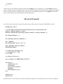
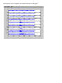
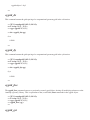
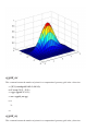
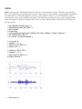
Advanced Example
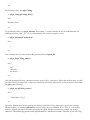
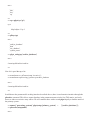
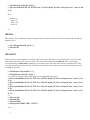
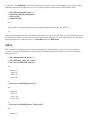
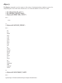
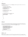
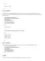
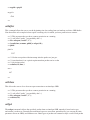
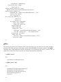
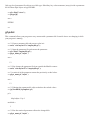
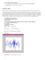
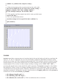
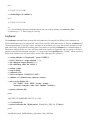
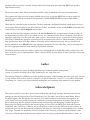
Get 100 seconds of data that occurred 10 minutes ago on the network of stations at Shishaldin volcano:
pf=dbpf(’aeic_rtsys’);
% Get the name of the current archive database from our local parameter file
primary = pfget(pf,’primary_system’);
dbname = pfresolve(pf,[’processing_systems{’ primary ’}{archive_database}’]);
db = dbopen( dbname, ’r’ );
db = dblookup_table( db, ’affiliation’ );
net = ’Shshldn’;
db = dbsubset(db, [’net == “’ net ’”’]);
dbw = dblookup_table( db, ’wfdisc’);
db=dbjoin(db, dbw);
% Get data from 10 minutes ago:
st = str2epoch(’now’) - 600;
et = st + 100;
tr = trload_css( db, st, et );
nrecs = dbquery( tr, ’dbRECORD_COUNT’);
for i=1:nrecs,
subplot( nrecs, 1, i )
tr.record=i-1;
data=trextract_data(tr);
plot(data)
ylabel(dbgetv(tr,’sta’));
end
trdestroy( tr );
dbclose( db );
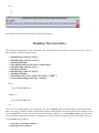
Channel names are not labelled. One station has three components, and another has both a vertical component
and a pressure sensor, explaining the repetition of names in this figure.
Examples of each command
Many of these presume you have run the command dbexample_get_demodb_path, which sets the variable
demodb_path to the name of a sample database. An attempt was made to make each of these examples selfsufficient. Hence there are usually a number of setup commands to make the example call possible. Some of
the examples may be a bit contrived. Note that in practice, it is not necessary to keep reopening a database
or a parameter-file object! The parameter-file routines use the dbloc2.pf and the rtexec.pf parameter files as
examples. They should be available on any properly installed Antelope system. There are also Matlab .m files
showing examples of each command in use. These example files should be in $ANTELOPE/data/matlab/
antelope/examples on a properly configured system. For a list of available examples, type help antelope/
examples.
abspath
The abspath command computes the absolute equivalent pathname from the filesystem root, to the file given as
argument:
>> abspath( ‘.’ )
ans =
/Users/kent
arr_slowness
The arr_slowness command calculates the slownesses of all known seismic phases, given the distance delta
in degrees to the earthquake and the depth of the earthquake in kilometers. The default travel-time model
is IASPEI ‘91, however this may be modified with the TAUP_TABLE environment variable. The returned
slowness values are in seconds/km.
>> delta = 20;
>> depth = 10;
>> [slowness, phasenames] = arr_slowness( delta, depth );
>> space(1:length(slowness),1) = ‘ ‘;
>> [num2str(slowness) space char(phasenames)]
ans =
0.097873 P
0.10638 Pn
0.097967 pP
0.097943 sP
0.10668 pPn
0.082873 P
0.1066 sPn
0.082883 pP
0.08288 sP
0.12307 PnPn
0.17998 S
0.21628 Sn
0.2027 S
0.21256 S
0.18023 sS
0.21638 sSn
0.20348 sS
0.21217 sS
0.14975 S
0.14986 pS
0.14981 sS
0.22062 SnSn
0.016438 PcP
0.021013 ScP
0.021017 PcS
0.030333 ScS
0.0039843 PKiKP
0.0039835 pPKiKP
0.0039837 sPKiKP
0.0042026 SKiKP
-0.0040705 PKKPdf
-0.0038634 SKKPdf
-0.0038632 PKKSdf
-0.0036761 SKKSdf
-0.0053076 P’P’df
-0.039783 P’P’ab
-0.0041508 S’S’df
>>
arrtimes
The arrtimes command calculates the travel-times of all known seismic phases, given the distance delta in
degrees to the earthquake and the depth of the earthquake in kilometers. The default travel-time model is
IASPEI ‘91, however this may be modified with the TAUP_TABLE environment variable. The returned traveltime values are in seconds. In this example, we feed the result to strtdelta to produce a more readable result.
>> delta = 20;
>> depth = 10;
>> [times, phasenames] = arrtimes( delta, depth );
>> [char(strtdelta(times)) char(phasenames)]
ans =
4:33 minutes
4:34 minutes
P
Pn
4:36 minutes
4:37 minutes
4:37 minutes
4:38 minutes
4:39 minutes
4:41 minutes
4:42 minutes
4:49 minutes
8:18 minutes
8:20 minutes
8:20 minutes
8:21 minutes
8:23 minutes
8:24 minutes
8:25 minutes
8:25 minutes
8:27 minutes
8:30 minutes
8:32 minutes
8:36 minutes
8:48 minutes
12:25 minutes
12:26 minutes
16:07 minutes
16:37 minutes
16:41 minutes
16:42 minutes
20:08 minutes
31:47 minutes
35:18 minutes
35:19 minutes
38:50 minutes
40:17 minutes
42:47 minutes
54:25 minutes
pP
sP
pPn
P
sPn
pP
sP
PnPn
S
Sn
S
S
sS
sSn
sS
sS
S
pS
sS
SnSn
PcP
ScP
PcS
ScS
PKiKP
pPKiKP
sPKiKP
SKiKP
PKKPdf
SKKPdf
PKKSdf
SKKSdf
P’P’df
P’P’ab
S’S’df
>>
cggrid
The cggrid command creates a Matlab object with references an Antelope computational-geomegry grid. This
command may be given one argument or three. A single argument will be interpreted as a filename, out of which
a previously saved grid will be retrieved. If three arguments are given, they should be matrices of X,Y, and Z
coordinate values for the grids, in the style of the Matlab mesh command.
>> [X,Y] = meshgrid(-2:0.2:2,-3:0.3:3);
>> Z = exp( -X.^2 - Y.^2 );
>> cgg = cggrid( X, Y, Z )
cgg =
cggrid object: 1-by-1
>>
cggrid_dx
This command returns the grid-spacing of a computational-geometry grid in the x direction:
>> [X,Y] = meshgrid(-2:0.2:2,-3:0.3:3);
>> Z = exp( -X.^2 - Y.^2 );
>> cgg = cggrid( X, Y, Z );
>> dx = cggrid_dx( cgg )
dx =
0.2000
>>
cggrid_dy
This command returns the grid-spacing of a computational-geometry grid in the y direction:
>> [X,Y] = meshgrid(-2:0.2:2,-3:0.3:3);
>> Z = exp( -X.^2 - Y.^2 );
>> cgg = cggrid( X, Y, Z );
>> dx = cggrid_dy( cgg )
dy =
0.3000
>>
cggrid_free
The cggrid_free command removes a previously created cggrid object, freeing all underlying references to the
Antelope cgeom(3) library. This is equivalent to the (overloaded) clear command for the cggrid object.
>> [X,Y] = meshgrid(-2:0.2:2,-3:0.3:3);
>> Z = exp( -X.^2 - Y.^2 );
>> cgg = cggrid( X, Y, Z );
>> cggrid_free( cgg )
>>
cggrid_get
The cggrid_get command returns a two-dimensional array of x,y, and z values for the specified grid. The
second and third return values are the number of points in the x and y directions, respectively (useful if one
wishes to call the reshape command on the result).
>> [X,Y] = meshgrid(-2:0.2:2,-3:0.3:3);
>> Z = exp( -X.^2 - Y.^2 );
>> cgg = cggrid( X, Y, Z );
>> [mytriplets, nx, ny] = cggrid_get( cgg );
>> whos mytriplets
Name
Size
mytriplets
441x3
Bytes Class
10584 double array
Grand total is 1323 elements using 10584 bytes
>> nx
nx =
21
>> ny
ny =
21
>>
cggrid_getmesh
The cggrid_getmesh command formats a cggrid object into three arrays of X,Y, and Z coordinate values,
suitable for direct use with the Matlab mesh, surf, and related commands.
>> [X,Y] = meshgrid(-2:0.2:2,-3:0.3:3);
>> Z = exp( -X.^2 - Y.^2 );
>> cgg = cggrid( X, Y, Z );
>> [myx, myy, myz] = cggrid_getmesh( cgg );
>> surf( myx, myy, myz )
>>
cggrid_nx
This command returns the number of points for a computational-geometry grid in the x direction:
>> [X,Y] = meshgrid(-2:0.2:2,-3:0.3:3);
>> Z = exp( -X.^2 - Y.^2 );
>> cgg = cggrid( X, Y, Z );
>> nx = cggrid_nx( cgg )
nx =
21
>>
cggrid_ny
This command returns the number of points for a computational-geometry grid in the y direction:
>> [X,Y] = meshgrid(-2:0.2:2,-3:0.3:3);
>> Z = exp( -X.^2 - Y.^2 );
>> cgg = cggrid( X, Y, Z );
>> ny = cggrid_ny( cgg )
ny =
21
>>
cggrid_probe
This command returns the value of a cggrid at a specified test point, or NaN if the test point is outside the grid.
If the test point does not lie exactly on a grid node, bilinear interpolation is used to extract the grid value.
>> [X,Y] = meshgrid(-2:0.2:2,-3:0.3:3);
>> Z = exp( -X.^2 - Y.^2 );
>> cgg = cggrid( X, Y, Z );
>> x_test = 1.138;
>> y_test = -2.045;
>> a_value = cggrid_probe( cgg, x_test, y_test )
a_value =
0.0047
>>
cggrid_write
The cggrid_write command sends a cggrid object to a filename in the specified format. The format is indicated
by a two-letter string, such as ‘as’ or ‘t4’, as documented in the Unix man-page cggrid(5).
>> [X,Y] = meshgrid(-2:0.2:2,-3:0.3:3);
>> Z = exp( -X.^2 - Y.^2 );
>> cgg = cggrid( X, Y, Z );
>> outfile = [’/tmp/mycggrid_’ getenv(’USER’)];
>> cggrid_write( cgg, ’t4’, outfile )
>>
cggrid2db
The cggrid2db command assumes the specified grid is associated with an earthquake. The database-pointer
provided must be aimed at a row containing the origin-time (‘time’) and origin-id (‘orid’) for the hypocenter.
The database must also contain a ‘qgrid’ table as in the gme1.0 database schema, to hold a reference to the
output qgrid file. The arguments to cggrid2db in the example below are, respectively, the input grid; the
database pointer containing information on the corresponding earthquake; the name of the recipe used to create
the grid; the name of the grid itself; a formatting string for the filename in which to save the grid; the format of
the grid; and the units of the grid (acceleration in g):
>> % Construct a contrived grid:
>> [X,Y] = meshgrid(-2:0.2:2,-3:0.3:3);
>> Z = exp( -X.^2 - Y.^2 );
>> cgg = cggrid( X, Y, Z );
>> % Save this to a fake database as though it belonged
>> % to an earthquake:
>> output_dir = [’/tmp/exampledir_’ getenv(’USER’)];
>> unix( [’/bin/rm -rf ’ output_dir] );
>> unix( [’mkdir ’ output_dir] );
>> output_dbname = [output_dir ’/newdb’];
>> fid = fopen( output_dbname, ’w’ );
>> fprintf( fid, ’#\nschema rt1.0:gme1.0\n’ );
>> fclose( fid );
>> db=dbopen( output_dbname,’r+’ );
>> db=dblookup( db,’’,’origin’,’’,’’ );
>> orid = dbnextid( db, ’orid’ );
>> db.record = dbaddv( db, ’lat’, -116, ...
’lon’, 34, ...
’depth’, 0, ...
’time’, str2epoch( ’12/31/2002’ ), ...
’orid’, orid, ...
’nass’, 0, ...
’ndef’, 0 );
>> cggrid2db( cgg, db, ’dbexample_fake’, ’testgrid’, ...
’%Y/%j/%{gridname}_%{recipe}.%{qgridfmt}’, ...
’t4’, ’g’, ‘pga’, ‘matlab_demo’ );
>>
clear_register
Most of the toolbox routines are pretty good about complaining of problems when they occur. However, if you
suspect the package is caching a useful error message, this is the way to bring them to the surface.
>> clear_register(’print’)
>>
>> % [...if there were error messages accumulated, this would have flushed them out...]
compare_response
The compare_response command may be used to compare the coefficients for two response objects, returning
a true value if they differ. In the following contrived example, two arbitrarily chosen response structures are
loaded and compared:
>> db = dbopen(demodb_path,’r’);
>> db=dblookup_table(db,’instrument’);
>> db.record=0;
>> file1=dbfilename(db);
>> resp1 = dbresponse(file1);
>> db.record=1;
>> file2=dbfilename(db);
>> resp2 = dbresponse(file2);>>
>> compare_response( resp1, resp2 )
1
>>
concatpaths
The concatpaths command assembles Unix pathname elements into a single composite path:
>> concatpaths( getenv(‘ANTELOPE’), ‘data’, ‘pf’ )
ans =
/opt/antelope/4.11/data/pf
datafile
The datafile command locates a private data file from the data subdirectory:
>> datafile( ‘’, ‘pf/rtexec.pf’ )
ans =
/opt/antelope/5.0-64/data/pf/rtexec.pf
datapath
The datapath command locates a private data file from the data subdirectory, with directory and suffix specified:
>> datapath( ‘’, ‘pf’, ‘rtexec’, ‘pf’ )
ans =
/opt/antelope/5.0-64/data/pf/rtexec.pf
db2struct
This is probably one of the more useful commands in the toolbox. It can operate on a database table or on a
view that contains only one table (for example, it will work on a view showing a subset of the origin table, but
not a view that was made by joining the origin and assoc tables).
>> db = dbopen(demodb_path,’r’);
>> db = dblookup_table( db, ’origin’ );
>> db.record=0;
>>
>> % Example 1:
>> db2struct(db)
ans =
lat: 40.0740
lon: 69.1640
depth: 155.1660
time: 7.0437e+08
orid: 1
evid: -1
jdate: 1992118
nass: 7
ndef: 7
ndp: -1
grn: 715
srn: 48
etype: ’-’
review: ’’
depdp: -999
dtype: ’f’
mb: 2.6200
mbid: 1
ms: -999
msid: -1
ml: -999
mlid: -1
algorithm: ’locsat:kyrghyz’
auth: ’JSPC’
commid: -1
lddate: 790466871
>>
>>
>> % Example 2:
>> db=dblookup(db,’’,’’,’’,’dbALL’);
>> db2struct(db)
ans =
1x1351 struct array with fields:
lat
lon
depth
time
orid
evid
jdate
nass
ndef
ndp
grn
srn
etype
review
depdp
dtype
mb
mbid
ms
msid
ml
mlid
algorithm
auth
commid
lddate
>>
>>
>> % Example 3:
>> db.record=0;
>> db2struct(db,’lat’,’lon’,’depth’,’mb’)
ans =
lat: 40.0740
lon: 69.1640
depth: 155.1660
mb: 2.6200
>>
dbadd
The raw storage format of the Datascope files is fixed-format ASCII rows. Usually, interaction with the database
tables is smoother if you avoid handling entire rows at once. However, there are occasions where it is useful
to move an entire row around. dbadd adds an entire database row to the flat-file table at once. The database
pointer for each table contains something called a ‘scratch’ record for that table. The scratch record is an entire
row that is in memory for the sole purpose of scribbling. In this example we add several values to the scratch
row of the origin table, then write the scratch row to the database (i.e. in this example that means we’ve written
the fixed-format ASCII row to the end of the file /tmp/newdb.origin).
>> db=dbopen(’/tmp/newdb’,’r+’);
>> db=dblookup(db,’’,’origin’,’’,’dbSCRATCH’);
>> dbputv(db,’lat’,61.5922,’lon’,-149.130,’depth’,20,’time’,str2epoch(’now’));
>> db.record=dbadd(db,’dbSCRATCH’)
db =
database: 0
table: 10
field: -501
record: 0
>>
dbadd_remark
The css3.0 schema, plus several other related schemas, have a separate table for comments. This table is
infrequently used. The dbadd_remark and dbget_remark functions encapsulate the operations involved in
adding a row to the remark table and linking it to a database row on another table such as the origin table..
>> db=dbopen(’/tmp/newdb’,’r+’);
>> db=dblookup_table(db,’origin’);
>> db.record = dbaddnull(db);
>> dbputv(db,’lat’,61.5922,’lon’,-149.130,’depth’,20,’time’,str2epoch(’now’))
>> dbadd_remark(db,’This earthquake occurred under Palmer, Alaska’)
>>
dbaddnull
Similar to dbadd, dbaddnull puts into a database table an entire fixed-format ASCII row, with format
appropriate for that table. In this case all the fields of the new row are set to their null values.
>> db=dbopen(’/tmp/newdb’,’r+’);
>> db=dblookup_table(db,’origin’);
>> db.record = dbaddnull(db)
db =
database: 0
table: 10
field: -501
record: 0
>>
dbaddv
This is one of the most commonly used functions in the Datascope libraries. dbaddv adds a new fixed-format
row to the specified table, setting all fields to their null values. It then modifies the specified fields to contain
the more interesting values given in each key-value pair. dbaddv checks to make sure none of the primary keys
match those for another row of the database, i.e. it takes some steps to keep you from corrupting your database.
>> db=dbopen(’/tmp/newdb’,’r+’);
>> db=dblookup_table(db,’origin’);
>> db.record=dbaddv(db,’lat’,61.5922,’lon’,-149.130,’depth’,20,’time’,str2epoch(’now’),’nass’,0,’nd
ef’,0)
db =
database: 0
table: 10
field: -501
record: 0
>>
dbclose
This routine closes a database pointer, freeing all the associated resources (It does no harm to the underlying
database files).
>> db = dbopen(demodb_path,’r’);
>> dbclose(db)
>>
dbcrunch
Removing rows from a database is usually done in two steps. The first is to set all the fields of a row to their
null values, but to leave the row in its place. This first step is performed by dbmark. The second stage,
accomplished by the dbcrunch command, is to actually remove the null rows from the database table. This
two-step procedure prevents skewing of all the record numbers for a table, often useful if the program is still
working on the table.
>> db=dbopen(’/tmp/newdb’,’r+’);
>> db=dblookup_table(db,’origin’);
>> % Add four copies of the same quake, all at slightly different times:
>>db.record=dbaddv(db,’lat’,61.5922,’lon’,-149.130,’depth’,20,’time’,str2epoch(’now’),’nass’,0,’nd
ef’,0)
>>db.record=dbaddv(db,’lat’,61.5922,’lon’,-149.130,’depth’,20,’time’,str2epoch(’now’),’nass’,0,’nd
ef’,0);
>>db.record=dbaddv(db,’lat’,61.5922,’lon’,-149.130,’depth’,20,’time’,str2epoch(’now’),’nass’,0,’nd
ef’,0);
>>db.record=dbaddv(db,’lat’,61.5922,’lon’,-149.130,’depth’,20,’time’,str2epoch(’now’),’nass’,0,’nd
ef’,0);
>>
>> db.record=1;
>> dbmark(db)
>> dbcrunch(db)
>> dbquery(db,’dbRECORD_COUNT’)
ans =
3
>>
dbdelete
This command immediately deletes a row from a database table.
>> db=dbopen(’/tmp/newdb’,’r+’);
>> db=dblookup_table(db,’origin’);
>> % Add four copies of the same quake, all at slightly different times:
>> db.record=dbaddv(db,’lat’,61.5922,’lon’,-149.130,’depth’,20,’time’,str2epoch(’now’),’nass’,0,’nd
ef’,0)
>>db.record=dbaddv(db,’lat’,61.5922,’lon’,-149.130,’depth’,20,’time’,str2epoch(’now’),’nass’,0,’nd
ef’,0);
>>db.record=dbaddv(db,’lat’,61.5922,’lon’,-149.130,’depth’,20,’time’,str2epoch(’now’),’nass’,0,’nd
ef’,0);
>>db.record=dbaddv(db,’lat’,61.5922,’lon’,-149.130,’depth’,20,’time’,str2epoch(’now’),’nass’,0,’nd
ef’,0);
>>
>> dbquery(db,’dbRECORD_COUNT’)
ans =
4
>> db.record=1;
>> dbdelete(db)
>> dbquery(db,’dbRECORD_COUNT’)
ans =
3
>>
dbeval
This command is a general-purpose calculator which has access to standard math commands, useful
seismological functions such as travel-time calculators, and to all the fields of a database view which is fed to
the command.
>> db = dbopen(demodb_path,’r’);
>> db=dblookup_table(db,’origin’);
>> dbs=dblookup_table(db,’site’);
>> db.record=0;
>> db=dbjoin(db,dbs);
>> db.record=0;
>> dbeval(db,’arrival(“PKiKP”)-time’)
ans =
982.2883
>>
>> dbeval(db,’distance(site.lat,site.lon,origin.lat,origin.lon)’)
ans =
27.4124
>>
dbextfile
In the css3.0 schema and related schemas, many times external files are referenced in tables by the two fields
dir and dfile. The dbextfile command combines these two fields into a full pathname, resolving all relative
pathnames into absolute pathnames as well as adjusting for the actual location of the database table. The
dbextfile command requires the name of the base table from which the dir and dfile fields should come. (Note
that in many cases, the simpler dbfilename command will suffice instead of dbextfile).
>> db = dbopen( demodb_path,’r’ );
>> db = dblookup_table( db, ’wfdisc’ );
>> dbt = dblookup_table( db, ’sensor’ );
>> db = dbjoin( db, dbt );
>> dbt = dblookup_table( db,’instrument’ );
>> db = dbjoin( db, dbt );
>> db.record=0;
>> dbextfile( db, ’instrument’ )
ans =
/usr/local/matlab/toolbox/antelope/examples/demodb/response/sts2_vel_RT72A.1
>> dbextfile( db, ’wfdisc’ )
ans =
/usr/local/matlab/toolbox/antelope/examples/demodb/wf/knetc/1992/138/210426/19921382155.15.CHM.
BHZ
>>
dbfilename
In the css3.0 schema and related schemas, many times external files are referenced in tables by the two fields
dir and dfile. The dbfilename command combines these two fields into a full pathname, resolving all relative
pathnames into absolute pathnames as well as adjusting for the actual location of the database table.
>> db = dbopen(demodb_path,’r’);
>> dblookup_table(db,’instrument’);
>> db.record=0;
>> dbfilename(db)
ans =
/opt/antelope/4.2u/data/matlab/antelope/examples/demodb/response/sts2_vel_RT72A.1
>>
Note that if more than one table with external file references is present in the input view, only the first one will
be chosen and returned. This may not always be the intended filename. For cases where the dir and dfile fields
appear multiple times in the input view, use dbextfile instead of dbfilename.
dbfind
This command is a general-purpose utility to hunt through a database table or view for a record matching
a specific criterion. Useful features include the ability to skip the first few matches, or to search backwards
through the view.
>> db = dbopen(demodb_path,’r’);
>> db = dblookup_table( db, ’origin’ );
>> db.record = dbfind(db,’mb>6’,0)
db =
database: 0
table: 10
field: -501
record: 80
>>
>> db.record = dbfind(db,’mb>6’,0,3)
db =
database: 0
table: 10
field: -501
record: 266
>>
>> db.record = dbfind(db,’mb>6’,’backwards’)
db =
database: 0
table: 10
field: -501
record: 1262
>>
>> dbgetv(db,’mb’)
ans =
6.1400
>>
dbfree
This command frees up the resources allocated when a new view is created. The input database pointer must
identify a single table, that is db.table and db.database should be valid. Generally, it is only necessary to
explicitly free database views when they are very large or many of them are made within the same program.
>> db = dbopen( demodb_path,’r’ );
>> dbarrival = dblookup_table( db,’arrival’ );
>> % Make a temporary view
>> dbtemp = dbsubset( dbarrival, ’sta == “AAK”’ );
>> % Get something out of the temporary view
>> dbgetv( dbtemp, ’deltim’ )
ans =
0.0980
2.1640
2.2220
>> % Free resources associated with the temporary view
>> dbfree( dbtemp );
>>
dbget
As explained for the dbadd command, the underlying storage of database tables is as fixed-format ASCII rows.
The dbget command can be used to retrieve an entire database row as a string (in fact, it is much more general,
allowing the retrieval of entire tables or just specific fields depending on the value of the database pointer).
Rather than trying to parse the output of dbget, use dbgetv to find specific pieces of information in a table or
database row.
>> db = dbopen(demodb_path,’r’);
>> db = dblookup_table( db, ’origin’ );
>> db.record=0;
>> dbget(db)
ans =
40.0740 69.1640 155.1660 704371900.66886
1
-1 1992118 7 7 -1
-999.0000 f 2.62
1 -999.00
-1 -999.00
-1 locsat:kyrghyz JSPC
790466871.00000
715
-1
48
>>
dbget_remark
As explained under dbadd_remark, dbget_remark eases the retrieval of comments in databases with the
css3.0 remark table.
>> db=dbopen(’/tmp/newdb’,’r+’);
>> db=dblookup_table(db,’origin’);
>> db.record = dbaddnull(db);
>> dbputv(db,’lat’,61.5922,’lon’,-149.130,’depth’,20,’time’,str2epoch(’now’))
>> dbadd_remark(db,’This earthquake occurred under Palmer, Alaska’)
>> dbget_remark(db)
ans =
This earthquake occurred under Palmer, Alaska
>>
dbgetv
The dbgetv command is one of the most frequently used commands in the Antelope programming environment.
With dbgetv one can get specific fields out of a database row. A unique characteristic of the Matlab-interface
dbgetv command is the ability to extract entire columns at once out of a database table.
>> db = dbopen(demodb_path,’r’);
>> db = dblookup_table( db, ’origin’ );
>> db.record=0;
>> [lat,lon,auth] = dbgetv(db,’lat’,’lon’,’auth’)
lat =
40.0740
lon =
69.1640
auth =
JSPC
>>
>> db = dbsubset(db,’mb>6’);
>> dbgetv(db,’mb’)
ans =
6.4200
6.4000
6.2000
6.2000
6.2300
6.4000
6.3100
6.0200
6.2800
6.5000
6.5700
6.1100
6.0500
6.2100
6.3000
6.3000
6.2700
6.1400
>>
dbgroup
The dbgroup command takes a sorted view and groups the records into ‘bundles’, clustering together all those
records that have the same values for the group fields. For example, in the operation below we take the arrival
table, sort it by station, and group arrivals together by station. This allows us to make an easy count of the
number of arrivals at each station, via the ‘count()’ function in dbeval. The input list of group fields should be a
cell-array of strings, hence the squiggly brackets in the dbgroup call below.
>> db = dbopen( demodb_path,’r’ );
>> db = dblookup_table( db, ‘arrival’ );
>> db = dbsort( db, ‘sta’ );
>> db = dbgroup( db, { ‘sta’ } );
>> % Find the number of arrivals at each station:
>> for i=1:dbnrecs(db)
db.record=i-1;
sta = dbgetv(db,’sta’);
narr = dbeval( db, ‘count()’ );
sprintf( ‘%s %d\n’, sta, narr )
>> end
ans =
AAK 3
ans =
CHM 2
ans =
EKS2 1
ans =
KBK 2
ans =
KMI 1
ans =
TKM 1
ans =
USP 2
dbinvalid
The database-pointer is actually a structure of four integers. There is an ‘invalid’ value for all of these which is
occasionally useful for tests or as the input to some commands.
>> db = dbinvalid
db =
database: -102
table: -102
field: -102
record: -102
>>
dbjoin
dbjoin allows the user to construct composite views in a relational database. Information in each table is crossreferenced according to its primary fields to construct a set of the corresponding, joined rows.
>> db = dbopen(demodb_path,’r’);
>> dbarrival=dblookup_table(db,’arrival’);
>> dbwfdisc=dblookup_table(db,’wfdisc’);
>> db=dbjoin(dbarrival,dbwfdisc)
db =
database: 0
table: 34
field: -501
record: -501
>>
dbjoin_keys
The standard Datascope join operations between database tables are accomplished by inferring the sensible join
keys with which to combine the two tables. dbjoin_keys explains which fields were used or will be used to
perform a join.
>> db = dbopen(demodb_path,’r’);
>> dbarrival=dblookup_table(db,’arrival’);
>> dbwfdisc=dblookup_table(db,’wfdisc’);
>>
>> % Example 1:
>> dbjoin_keys(dbarrival,dbwfdisc)
ans =
’sta’
’time == time::endtime’
>>
>> % Example 2:
>> dbjoin_keys(db,’origin’,’assoc’)
ans =
’orid’
>>
dblist2subset
Normally, database views are created with commands such as dbsubset, dbsort, dbjoin, dbunjoin, etc., which
perform operations on one or more views to create a new view. However, sometimes one encounters situations
where one knows the exact row numbers of interest for an existing view and wants to create a new view
containing just those rows. For this purpose there is the dblist2subset command. Given an array of numbers
specifying the row numbers to include, dblist2subset will create a new view. The example below shows this in
use with the trload_css command. Since the trload_css command ignores the actual record-number field of the
input database pointer, a preceding dblist2subset call can restrict the input view to just one or several rows of
interest (if several rows are desired, instead of just one as in the example below, the row numbers should be put
into a single Matlab vector which is then given to dblist2subset as its second argument). The dblist2subset can
also be called without a second argument, in which case dblist2subset assumes the database pointer refers to a
group (as created by the dbgroup command) and turns the group into a proper view of its own.
>> db = dbopen( demodb_path,’r’ );
>> db=dblookup_table( db,’wfdisc’ );
>> db.record=3;
>> format long
>> [time,endtime,nsamp,samprate]=dbgetv( db,’time’,’endtime’,’nsamp’,’samprate’ )
time =
7.061397047000000e+08
endtime =
7.061398015500000e+08
nsamp =
1938
samprate =
20
>> % The trload_css command by itself ignores the record number of the
>> % database pointer, loading everything it finds in the input table.
>> % the dblist2subset command below creates a subset view the consists solely
>> % of the record of interest, thus limiting the amount of data loaded by the
>> % command. Note that this strategy assumes all the data of interest
>> % exist in the row being pointed to, which may or may not defeat the strength
>> % of the trload_css command, depending on the application. At the very least
>> % one may wish to include all relevant wfdisc row numbers in the list fed
>> % to dblist2subset, in which case a simple dbsubset command might be less
>> % effort to design.
>>
>> db = dblist2subset( db, 3 );
>> tr = trload_css( db,time,endtime );
>> tr.record = 0;
>> data = trextract_data( tr );
>>
>> % Do something interesting (or, in this case, boring) with the data:
>> mean( data )
ans =
-6.830181208053691e+03
>> dbclose( db );
>> trdestroy( tr );
dblookup
The four-element dbpointer structure, used as a handle to reference different fields or sections of a relational
database, is rarely modified by hand. dblookup allows the four elements of the dbpointer structure to be aimed
based on human-readable names for the tables and fields. Additionally, several recognized constants such as
‘dbALL’ and ‘dbSCRATCH’ allow further control of the parts of the database to which dblookup aims the
database pointer.
>> db = dbopen(demodb_path,’r’);
>> dblookup(db,’’,’origin’,’’,’dbALL’)
ans =
database: 0
table: 10
field: -501
record: -501
>>
dblookup_table
One of the most common operations with dblookup is to aim the database pointer at a particular table.
dblookup_table is an easier-to-type shorthand for this operation.
>> db = dbopen(demodb_path,’r’);
>> db = dblookup_table(db,’origin’)
db =
database: 0
table: 10
field: -501
record: -501
>>
dbmark
This command is the first stage of a two-part process to remove a row from a database table, as explained under
dbcrunch. For the impatient, see dbdelete.
>> db=dbopen(’/tmp/newdb’,’r+’);
>> db=dblookup_table(db,’origin’);
>> % Add four copies of the same quake, all at slightly different times:
>> db.record=dbaddv(db,’lat’,61.5922,’lon’,-149.130,’depth’,20,’time’,str2epoch(’now’),’nass’,0,’nd
ef’,0)
>>db.record=dbaddv(db,’lat’,61.5922,’lon’,-149.130,’depth’,20,’time’,str2epoch(’now’),’nass’,0,’nd
ef’,0);
>>db.record=dbaddv(db,’lat’,61.5922,’lon’,-149.130,’depth’,20,’time’,str2epoch(’now’),’nass’,0,’nd
ef’,0);
>>db.record=dbaddv(db,’lat’,61.5922,’lon’,-149.130,’depth’,20,’time’,str2epoch(’now’),’nass’,0,’nd
ef’,0);
>>
>> db.record=1;
>> dbmark(db)
>>
dbnextid
In several of the css3.0-style database tables, entries such as hypocentral solutions (“origin” table) or seismic
phase arrivals (“arrival” table) are identified with unique, integer id’s. The dbnextid command allows the
retrieval of the next unused value for any of these integer indices.
>> db=dbopen(’/tmp/newdb’,’r+’);
>> dbnextid(db,’orid’)
ans =
1
>>
dbnojoin
Similar to dbjoin, the dbnojoin command returns a view showing rows in the first table that have no
counterpart in the second.
>> db = dbopen(demodb_path,’r’);
>> dbarrival=dblookup_table(db,’arrival’);
>> dbwfdisc=dblookup_table(db,’wfdisc’);
>> db=dbnojoin(dbarrival,dbwfdisc)
db =
database: 0
table: 36
field: -501
record: -501
>>
dbnrecs
The dbnrecs command returns the number of records in a database table or view.
>> db = dbopen( demodb_path,’r’ );
>> db = dblookup_table( db,’origin’ );
>> nrecs = dbnrecs( db )
nrecs =
1351
>>
dbopen
The first step in using Datascope on a relational database is to create a ‘handle’, called a database pointer, to the
ASCII flat files which store the database contents. This step is performed by dbopen. Here we have written a
small routine to reliably provide the pathname of a sample database for these examples.
>> dbexample_get_demodb_path
demodb_path =
/opt/antelope/4.2u/data/matlab/antelope/examples/demodb/demo
>> db = dbopen(demodb_path,’r’)
db =
database: 0
table: -501
field: -501
record: -501
>>
dbpf
Many programs require some form of parameter file to store information about run-time configuration. The
Antelope parameter-file utility provides a very powerful mechanism to handle such input files, including
boolean, string, and numeric values as well as tables or key-value arrays, all of which can be nested. In the
Antelope Toolbox for Matlab, interaction with a parameter file is through a ‘handle’ called a dbpf object. See the
Antelope documentation for more details on the parameter file mechanism.
>> pf = dbpf( ’dbloc2’ )
pf =
dbpf object: 1-by-1
>> % Now as a contrived example of the other methods of use,
>> % convert it to a string, then compile it into a new parameter-file object:
>> string_version = pf2string( pf );
>> % Create an empty parameter-file object:
>> newpf = dbpf
newpf =
dbpf object: 1-by-1
>> % Compile the new string into the empty parameter-file object:
>> % (you can compile into parameter-file objects that aren’t empty as well)
>> newpf = dbpf( newpf, string_version)
newpf =
dbpf object: 1-by-1
>>
dbprocess
Dbprocess provides a simplified interface for forming various views. When a sequence of standard database
operations (such as subsets, joins, sorts, etc.) need to be performed all in a row, they can be combined into a
single block, passed as a list of statements to dbprocess.
>> db = dbopen( demodb_path,’r’ );
>> db = dbprocess( db, { ’dbopen arrival’;
’dbsubset sta == “AAK”’;
’dbjoin assoc’ } );
>> [iphase, delta] = dbgetv( db,’iphase’, ’timeres’ )
iphase =
’P’
’S’
delta =
-0.0500
0.8600
>>
Detailed explanations of the valid statements available in dbprocess may be found in the unix man-pages for the
dbprocess command. For reference, a summary list is provided here:
dbopen table
dbjoin [-o] table [ key key ..]
dbgroup key [ key ..]
dbleftjoin [-o] table [ key key ..]
dbnojoin table [ key key ..]
dbselect expr [expr ...]
dbseparate table
dbsever table
dbsort [-ru] key .. ]
dbsubset expression
dbtheta table [ expression ..]
dbungroup
dbput
This function is similar to dbput, however it does not automatically add its own null row. Also, it does not do
any consistency checking to make sure the new row makes sense given the contents of the rest of the table.
Again, avoid working with entire rows at once unless necessary. Consider using dbputv if possible.
>> db=dbopen(’/tmp/newdb’,’r+’);
>> db=dblookup_table(db,’origin’);
>> db.record = dbaddnull(db);
>> dbputv(db,’lat’,61.5922,’lon’,-149.130,’depth’,20,’time’,str2epoch(’now’))
>> record = dbget(db)
record =
61.5922 -149.1300 20.0000 923760231.63253
-999.0000 - -999.00
-1 -999.00
-1 -999.00
-1
-1 -
-1
-1 -1 -1 -1
-1
-1 - -1 923760231.66952
>>
>> db.record = dbaddnull(db);
>> dbput(db,record)
>>
dbputv
The dbputv command is used to put individual field values into a database row. This is an extremely important
command in the Datascope library. Here, we make a new row with the dbaddnull command so we have
somewhere to put our values.
>> db=dbopen(’/tmp/newdb’,’r+’);
>> db=dblookup_table(db,’origin’);
>> db.record = dbaddnull(db);
>> dbputv(db,’lat’,61.5922,’lon’,-149.130,’depth’,20,’time’,str2epoch(’now’),’nass’,0,’ndef’,0)
>>
dbquery
The dbquery command is used to request a wide variety of information about a database or one of its
component parts. One of the most common uses is to count the number of records in a a table.
>> db = dbopen(demodb_path,’r’);
>> db = dblookup_table(db,’origin’);
>> dbquery(db,’dbRECORD_COUNT’)
ans =
1351
>>
>> dbquery(db,’dbTABLE_FIELDS’)
ans =
’lat’
’lon’
’depth’
’time’
’orid’
’evid’
’jdate’
’nass’
’ndef’
’ndp’
’grn’
’srn’
’etype’
’review’
’depdp’
’dtype’
’mb’
’mbid’
’ms’
’msid’
’ml’
’mlid’
’algorithm’
’auth’
’commid’
’lddate’
>>
>> dbquery(db,’dbDATABASE_NAME’)
ans =
/opt/antelope/4.2u/data/matlab/antelope/examples/demodb/demo
>>
dbread_view
dbread_view is a less common command, used to read a view out of a file (for example, out of the file saved by
dbsave_view). An example of that straightforward usage is shown in the script dbexample_dbread_view.m.
For the tutorial we will show a far more unconventional use just to add interest. We will create a named-pipe
with the unix mkfifo(1) command, then write to that pipe by calling the command-line version of dbsubset [Note
for the advanced that it’s necessary to do that in the background when using the Matlab unix() command, since
the pipe will not close until the other end is read and flushed]. Then we get the database view out of the pipe and
into Matlab with the dbread_view command:
>> unix(’mkfifo /tmp/mypipe’);
>> unix([’dbsubset ’ demodb_path ’.origin “ms > 6.8” > /tmp/mypipe &’]);
>> db = dbread_view( ’/tmp/mypipe’ )
db =
database: 3
table: 45
field: -501
record: -501
>> dbgetv( db, ’ms’ )
ans =
7.1000
7.5000
6.9000
7.0000
>>
dbresponse
The css3.0 schemas and related schemas reference instrument response information in separate files. These
response files allow poles-and-zeros format, frequency-amplitude-phase triplet format, FIR format, and more.
The dbresponse object is a handle to one of these response files, from which response information can be
extracted.
>> db = dbopen(demodb_path,’r’);
>> db=dblookup_table(db,’instrument’);
>> db.record=0;
>> file=dbfilename(db)
file =
/opt/antelope/4.2u/data/matlab/antelope/examples/demodb/response/sts2_vel_RT72A.1
>>
>> resp = dbresponse(file)
resp =
dbresponse object: 1-by-1
>>
dbsave_view
dbsave_view takes a current view into a database and saves it as though it were a base table of the main
database. This is useful if a lot of processing was necessary to create the original view. Note that because the
Antelope Toolbox for Matlab does not currently support named views, the name of the saved view will default
to the name assigned by Datascope. However, once the database is closed the file may be moved to a new name.
Also note that saved views are binary files of indexes. The dbe program should be used to view them. Views
will become stale if any of the component tables change. To make an example of this command, we will copy
the necessary parts of the demo database, make a joined view, and save it:
>> output_dbname = [‘/tmp/newdb_’ getenv(‘USER’)];
>> unix( [’cp ’ demodb_path ’.arrival ’ output_dbname ’.arrival’] );
>> unix( [’cp ’ demodb_path ’.wfdisc ’ output_dbname ’.wfdisc’] );
>> db = dbopen( output_dbname,’r’ );
>> dbarrival=dblookup_table( db,’arrival’ );
>> dbwfdisc=dblookup_table( db,’wfdisc’ );
>> db=dbjoin( dbarrival,dbwfdisc );
>> dbsave_view( db );
>>
dbseparate
dbseparate extracts the rows from the specified base table that participate in a given view. For example, we can
start with a whole set of wfdisc records, construct a view that joins them ultimately to hypocentral information,
subset for a hypocenter of interest, and then extract the resulting wfdisc records which have matched:
>> db = dbopen( demodb_path,’r’ );
>> db = dbprocess( db, { ‘dbopen wfdisc’; ...
‘dbjoin arrival’; ...
‘dbjoin assoc’; ...
‘dbjoin origin’; ...
‘dbsubset orid == 645’ } );
>> db = dbseparate( db, ‘wfdisc’ );
>> db.record=0;
>> dbextfile( db, ‘wfdisc’ )
ans =
/opt/antelope/data/db/demo/wf/knetc/1992/138/210426/19921382155.15.CHM.BHZ
>>
For brevity, we have only printed one of the resulting file names from the records this retrieved.
dbsever
The dbsever command takes an existing view and removes an unwanted or no-longer needed table from that
view. The returned value is a view without any fields from the removed table. If necessary, the resulting view is
condensed to eliminate any duplicate rows.
>> db = dbopen( demodb_path,’r’ );
>> dborigin=dblookup_table( db,’origin’ );
>> dbstamag=dblookup_table( db,’stamag’ );
>> db=dbjoin( dborigin, dbstamag );
>> % Get rid of the stamage values now that we know which orids have stamags:
>> db= dbsever( db, ‘stamag’ )
db =
database: 1
table: 46
field: -501
record: -501
>> dbgetv( db, ‘orid’ )
ans =
645
>>
dbsort
This command takes any database view and returns a view sorted according to the specified expression.
>> db = dbopen(demodb_path,’r’);
>> db=dblookup_table(db,’origin’);
>> db=dbsubset(db,’mb>6.3’);
>> db=dbsort(db,’mb’);
>> dbgetv(db,’mb’)
ans =
6.3100
6.4000
6.4000
6.4200
6.5000
6.5700
>>
If one of the arguments to dbsort is ‘dbSORT_UNIQUE’, the view returned will have only one representative
for each unique value of the sort field(s). I.e. rows which have duplicate sort keys will be eliminated. If one of
the arguments is ‘dbSORT_REVERSE’, the sort will be performed in reverse order.
dbsubset
This command, fairly self-explanatory, returns a database view containing only those rows from the input view
which match the specified expression.
>> db = dbopen(demodb_path,’r’);
>> db=dblookup_table(db,’origin’);
>> db=dbsubset(db,’mb>6.3’);
>> dbgetv(db,’mb’)
ans =
6.4200
6.4000
6.4000
6.3100
6.5000
6.5700
>>
dbtheta
In the dbjoin command, specified above, the comparison fields (“join keys”) used to describe which rows
correspond were inferred. The dbtheta command allows you to perform the join with full command over
whether or not two rows should be associated together or not, based on the supplied test expression.
>> db = dbopen(demodb_path,’r’);
>> dbassoc = dblookup_table(db,’assoc’);
>> dbwfdisc = dblookup_table(db,’wfdisc’);
>> db=dbtheta(dbassoc,dbwfdisc,’assoc.sta == wfdisc.sta’)
db =
database: 0
table: 45
field: -501
record: -504
>>
dbungroup
The dbungroup command is the inverse of the dbgroup command. It unpacks a bundle of rows into a view
containing the individual rows.
>> db = dbopen( demodb_path,’r’ );
>> db = dblookup_table( db, ‘arrival’ );
>> db = dbsort( db, ‘sta’ );
>> db = dbgroup( db, { ‘sta’ } );
>> % Subset for one station:
>> db = dbsubset( db, ‘sta == “AAK”’ );
>> db = dbungroup( db );
>> % Get the arriving phases detected at this station:
>> db = dblookup( db, ‘’, ‘’, ‘’, ‘dbALL’ );
>> dbgetv( db, ‘iphase’ )
ans =
‘S’
‘P’
‘del’
>>
dbunjoin
Once a view is created, many database operations can be performed on it which winnow out certain rows of
each component table. The resulting view may be split into the component rows from each participating table
and written to a new database. This is accomplished with the dbunjoin command.
>> db = dbopen(demodb_path,’r’);
>> dbarrival=dblookup_table(db,’arrival’);
>> dbwfdisc=dblookup_table(db,’wfdisc’);
>> db=dbjoin(dbarrival,dbwfdisc);
>> dbunjoin(db,’/tmp/newdb’);
>> !ls /tmp/newdb*
/tmp/newdb.arrival /tmp/newdb.wfdisc
>>
dbwrite_view
dbwrite_view writes a database view to a file. This can be used in a number of ways, for example to pipe a
view to an external command (such as dbe(1)) via a named pipe. First we will set up the named pipe, and set up
the Antelope dbe program (running in the background) waiting for input from the pipe. Then we will create our
customized view in Matlab. Finally, we will write our view to the named pipe (which, like everything in unix,
just looks like a file). At that point dbe will receive its input
>> pipe_name = [’/tmp/mypipe_’ getenv(’USER’)];
>> unix( [’mkfifo ’ pipe_name] );
>> unix( [’cat ’ pipe_name ’ | dbe - &’] );
>> db = dbopen( demodb_path,’r’ );
>> dbarrival=dblookup_table( db,’arrival’ );
>> dbwfdisc=dblookup_table( db,’wfdisc’ );
>> db=dbjoin( dbarrival,dbwfdisc );
>> dbwrite_view( db, pipe_name );
>>
This causes a dbe(1) window to appear, showing the view that was calculated in Matlab.
elog_alert
The elog_alert function sends a message of severity ‘alert’ to the Antelope elog facility.
>> elog_alert( ‘This is an Antelope alert message’ )
Matlab *alert*: This is an Antelope alert message
>>
elog_complain
The elog_complain function sends a message of severity ‘complain’ to the Antelope elog facility.
>> elog_complain( ‘This is an Antelope complain message’ )
Matlab: This is an Antelope complain message
>>
elog_debug
The elog_debug function sends a message of severity ‘debug’ to the Antelope elog facility.
>> elog_debug( ‘This is an Antelope debug message’ )
Matlab *debug*: This is an Antelope debug message
>>
elog_die
The elog_die function sends a message of severity ‘die’ to the Antelope elog facility, then kills the Matlab
interpreter.
>> elog_die( ‘This is an Antelope die message’ )
Matlab *fatal*: This is an Antelope die message
%
elog_flush
The elog_flush routine eliminates log messages after the specified message number (the second argument),
printing them if the deliver argument (the first argument) is set to a nonzero value.
>> elog_log( ‘This is an Antelope log message’ )
>> elog_flush( 1, 0 )
Matlab: This is an Antelope log message
>>
elog_init
The elog_init routine initializes the Antelope error-logging facility. This should be called prior to using any of
the elog* routines. If no arguments are specified, the error logger is initialized with the program name set to
‘Matlab’. Otherwise, a single string may be specified, usually with the script name, which will be used in all the
output error messages as the name of the invoking program.
>> elog_init()
or
>> elog_init( ‘myscript’ )
elog_log
The elog_log function sends a message of severity ‘log’ to the Antelope elog facility.
>> elog_log( ‘This is an Antelope log message’ )
>>
elog_mark
The elog_mark routine returns the count of messages currently held in the error log.
>> elog_log( ‘This is an Antelope log message’ )
>> n = elog_mark()
n=
1
elog_notify
The elog_notify function sends a message of severity ‘notify’ to the Antelope elog facility.
>> elog_notify( ‘This is an Antelope notify message’ )
Matlab: This is an Antelope notify message
>>
elog_string
The elog_string function returns a string with the error log contents, starting with the specified message number
(message numbering starts at 0, so use 0 as the argument to retrieve all messages currently in the message
queue).
>> elog_log( ‘This is an Antelope log message’ )
>> logstring = elog_string( 0 )
logstring =
Matlab: This is an Antelope log message
>>
epoch2str
Most time handling in Antelope (not to mention Unix) is done in terms of Unix epoch seconds, or seconds
since 1970. The epoch2str command provides a highly flexible method for creating more human-readable time
strings from an epoch time.
>> now = str2epoch(’now’)
now =
9.237062953704129e+08
>> epoch2str( now, ’%D %H:%M:%S %Z’)
ans =
4/10/99 01:04:55 UTC
>> epoch2str( now, ’%A, %B %d %Y’)
ans =
Saturday, April 10 1999
>>
>> epoch2str( now, ’%G %l %p’)
ans =
1999-04-10 1 AM
>>
eval_response
This function allows a dbresponse object (ultimately, a file of instrument response information stored as
poles and zeroes or frequency-amplitude-phase triplets etc.) to be queried for the complex response at certain
frequency values.
>> db = dbopen(demodb_path,’r’);
>> db=dblookup_table(db,’instrument’);
>> db.record=0;
>> file=dbfilename(db);
>> resp = dbresponse(file);
>> eval_response(resp,6.28)
ans =
1.0008 - 0.0041i
>>
>> eval_response(resp,transpose([0.01 0.1 1 10])*6.28)
ans =
0.2550 + 0.8025i
0.9936 + 0.1116i
1.0008 - 0.0041i
0.0000 - 0.0000i
>>
free_response
Once the user is done with a dbresponse object, it must be freed with the free_response command.
>> db = dbopen(demodb_path,’r’);
>> db=dblookup_table(db,’instrument’);
>> db.record=0;
>> file=dbfilename(db);
>> resp = dbresponse(file);
>> free_response( resp )
>>
getpid
Get the system process-id of the Matlab interpreter from which this was called:
>> mypid = getpid
mypid =
4764
>>
orbafter
This command allows the user to set the beginning time for reading from an Antelope real-time ORB buffer.
Note that all the orb examples below require a running orb, for which you have permission to connect.
>> % This presumes that you have connect permission to a running
>> % orb called ’nordic’ (you probably don’t...)
>> fd = orbopen( ’nordic’, ’r’ );
>> [result,time, srcname, pktid] = orbget( fd );
>> pktid
pktid =
2357
>> % Get the next packet with timestamp after the packet we just got:
>> % (note that there’s no a-priori requirement that packets arrive on the
>> % orb in time order)
>> orbafter( fd, time )
ans =
497
>>
orbclose
This allows the user to close down an open connection to an Antelope ORB.
>> % This presumes that you have connect permission to a running
>> % orb called ’nordic’ (you probably don’t...)
>> fd = orbopen( ’nordic’, ’r’ );
>> orbclose( fd )
>>
orbget
The orbget command collects the specified packet from an Antelope ORB, unpacks it based on its type,
and returns it to the user. Currently the understood types are waveform, parameter-file (you can put an entire
parameter file on an ORB), and database-row. Other types of packets are returned as byte vectors. Each packet
on an orb has a timestamp and a source-name, which are also returned.
>> % This presumes that you have connect permission to a running
>> % orb called ’nordic’ (you probably don’t...)
>>
>> % First we’ll get a waveform-data object from an orb:
>> fd = orbopen( ’nordic’, ’r’ );
>> orbreject( fd, ’/db/.*|/pf/.*’ );
>> [result, time, srcname, pktid, type] = orbget( fd )
result =
database: 16
table: 5
field: -501
record: 0
time =
9.4638e+08
srcname =
AT_MID_SHZ
pktid =
724328
type =
waveform
>> result.record = 0;
>> plot( trextract_data( result ) );
>> trdestroy( result );
>> orbclose( fd );
>> % Now get a database-row object from an orb:
>> fd = orbopen(’megathrust’,’r’);
>> orbselect(fd,’/db/.*’);
>> orbseek(fd,’ORBOLDEST’);
>> result=orbget(fd)
result =
database: 0
table: 19
field: -501
record: -504
>> [lat,lon,mb]=dbgetv(result,’lat’,’lon’,’ml’)
lat =
59.8962
lon =
-152.0661
mb =
1.8600
>> % Finally, get a parameter-file object from an orb:
>> orbselect(fd,’/pf/.*’);
>> orbseek(fd,’ORBOLDEST’);
>> result=orbget(fd)
result =
dbpf object: 1-by-1
>> pf2string(result)
ans =
cmdstring
“echo hi | mail kent”
>>
orbopen
The orbopen command allows you to establish a read or write connection to a running Antelope ORB server
anywhere on the internet (provided the orbserver maintainers have given you permission to connect to that orb).
You may have multiple connections at once to the same ORB.
>> % This presumes that you have connect permission to a running
>> % orb called ’nordic’ (you probably don’t...)
>> fd = orbopen( ’nordic’, ’r’ )
fd =
21
>>
orbping
This command is primarily useful to verify that an ORB connection is up and running. It has the side benefit of
telling you the version number of the orbserver.
>> % This presumes that you have connect permission to a running
>> % orb called ’nordic’ (you probably don’t...)
>> fd = orbopen( ’nordic’, ’r’ );
>> orbping( fd )
ans =
6
>>
orbreap
This is one of the most common orb commands. Evaluated in a tight loop, it allows you to successively receive
packet after packet for the streams you’ve chosen. Each packet can then be processed as necessary.
>> % This presumes that you have connect permission to a running
>> % orb called ’nordic’ (you probably don’t...)
>> fd = orbopen( ’nordic’, ’r’ );
>> for i = 1:3,
[result,time,srcname] = orbreap( fd );
srcname
end
srcname =
AK_MDM_SHZ
srcname =
AK_KTH_SHZ
srcname =
AK_MCK_SHZ
>>
orbreject
This command allows the user to reject certain packets from ever coming across a particular orb connection.
The specification is by means of regular-expression matching on the source-names of the packets.
>> % This presumes that you have connect permission to a running
>> % orb called ’nordic’ (you probably don’t...)
>> fd = orbopen( ’nordic’, ’r’ );
>> % Reject all parameter-file packets, all database-row packets,
>> % and all waveform packets for the Alaska net whos station-names
>> % start with A,B, or C:
>> % (return the number of sources still available on the connection)
>> orbreject( fd, ’/db/.*|/pf/.*|AK_[A-C].*’ )
ans =
276
>>
orbseek
For a given read connection to an orbserver, the orbseek command allows the user to position the reading point
in the stream to a certain packet number or to a specified relative location in the stream (newest packet, oldest
packet, next packet, etc.).
>> % This presumes that you have connect permission to a running
>> % orb called ’nordic’ (you probably don’t...)
>> fd = orbopen( ’nordic’, ’r’ );
>> orbseek( fd, ’ORBOLDEST’ )
ans =
790548
>> orbseek( fd, ’ORBNEXT’ )
ans =
790549
>> orbseek( fd, ’ORBNEWEST’ )
ans =
321046
>> orbseek( fd, ’ORBPREV’ )
ans =
321045
>> orbseek( fd, ’ORBPREV’ )
ans =
321044
>> mypktid = orbtell( fd )
mypktid =
321044
>> orbseek( fd, ’ORBPREV’ )
ans =
321043
>> orbseek( fd, mypktid )
ans =
321044
>>
orbselect
Orbselect is a very useful command which allows the user to filter packets from an orb connection so that only
those matching certain source-name criteria get through.
>> fd = orbopen( ’nordic’, ’r’ );
>> % Choose all components of station DIV (Divide, Alaska)
>> % Return the number of selected sources
>> orbselect( fd, ’AK_DIV_.*’ )
ans =
3
>>
orbtell
This command returns the packet-identification-number for the current packet on read connection to an
orbserver.
>> % This presumes that you have connect permission to a running
>> % orb called ’nordic’ (you probably don’t...)
>> fd = orbopen( ’nordic’, ’r’ );
>> % Find the packet-id for the current packet:
>> orbtell( fd )
ans =
377956
>>
parse_response
The parse_response command takes a dbresponse object and expands it into its component filter stages and
filter coefficients. The result is returned as a cell array. Each cell in the cell array contains one stage of the
filter, represented as a Matlab structure. The field names in the structure vary according to the type of the filter,
although all of the structures have a ‘type’ field listing the type of the filter. For example, a filter stage of type
‘paz’ (poles and zeroes) will have vectors of the poles and zeros for the filter stage. A filter stage of type ‘fap’
(frequency-amplitude-phase) will have vectors of the frequency-amplitude-phase triplets.
>> db = dbopen( demodb_path,’r’ );
>> db=dblookup_table( db,’instrument’ );
>> db.record=0;
>> file=dbfilename( db );
>> resp = dbresponse( file );
>> parsed = parse_response( resp )
parsed =
[1x1 struct]
[1x1 struct]
[1x1 struct]
[1x1 struct]
[1x1 struct]
>> % Display the results:
>> celldisp( parsed )
parsed{1} =
type: ‘paz’
npoles: 2
nzeros: 2
normalization: 1
frequency: 0
poles: [2x1 double]
pole_errors: [2x1 double]
zeros: [2x1 double]
zero_errors: [2x1 double]
parsed{2} =
type: ‘paz’
npoles: 6
nzeros: 0
normalization: 1.5020e+19
frequency: 0
poles: [6x1 double]
pole_errors: [6x1 double]
zeros: []
zero_errors: []
parsed{3} =
type: ‘fir’
nnum: 99
nden: 1
srate: 1000
dec_factor: 5
seed_dec_offset: 0
midpoint: -1
num_coefs: [99x1 double]
num_coef_errors: [99x1 double]
den_coefs: 1
den_coef_errors: 0
parsed{4} =
type: ‘fir’
nnum: 95
nden: 1
srate: 200
dec_factor: 2
seed_dec_offset: 0
midpoint: -1
num_coefs: [95x1 double]
num_coef_errors: [95x1 double]
den_coefs: 1
den_coef_errors: 0
parsed{5} =
type: ‘fir’
nnum: 235
nden: 1
srate: 100
dec_factor: 5
seed_dec_offset: 0
midpoint: -1
num_coefs: [235x1 double]
num_coef_errors: [235x1 double]
den_coefs: 1
den_coef_errors: 0
>> % Display one of the component vectors:
>> parsed{1}.poles
ans =
-0.0355 + 0.0355i
-0.0355 - 0.0355i
>>
parsepath
parsepath separates a pathname into its component parts. This is done entirely by text analysis of the input
string, without any regard to whether the files, directories, or whatever they are actually exist. If the third output
argument is specified, any suffix is separated from the basename of the file. Otherwise the file basename is left
intact with any suffix.
>> [dir, base] = parsepath( ’/home/kent/testfile.txt’ )
dir =
/home/kent
base =
testfile.txt
>> [dir, base, suffix] = parsepath( ’/home/kent/testfile.txt’ )
dir =
/home/kent
base =
testfile
suffix =
txt
>>
pf2string
An entire parameter file (being essentially an ASCII file) or subsection thereof may be converted to a string.
>> pf=dbpf(’dbfixids’);
>> pf2string(pf)
ans =
css3.0 &Arr{
aliases &Arr{
magid mbid msid mlid
orid prefor
}
}
rt1.0 &Arr{
aliases &Arr{
magid mbid msid mlid
orid prefor
}
}
>>
pf2struct
The Matlab Antelope Toolbox allows an entire parameter file to be loaded into a Matlab struct. A Matlab
struct has strong similarity to the data storage in a parameter file: namely a flexible set of key-value pairs. The
‘recursive’ option to pf2struct can be used to read a complex parameter file all at once into an easy-to-use
Matlab-style object. This command can be extremely useful in making the entire contents of a parameter file
available in one clean strike, rather than multiple independent pfget calls. With pf2struct in ‘recursive’ mode,
one call converts every parameter in the parameter file into a like-named element of the returned structure.
Parameter values that appear to be numeric will be converted to numbers via the Matlab str2double function
[note that this is a change from earlier version of the Antelope Toolbox for Matlab]:
>> pf=dbpf(’dbloc2’);
>> pf2struct(pf)
ans =
Define: [1x1 dbpf]
Processes: [1x1 dbpf]
Run: [1x1 dbpf]
State: [1x1 dbpf]
User: [1x1 dbpf]
>>
>> pf2struct(pf,’recursive’)
ans =
Define: [1x1 struct]
Processes: [1x1 struct]
Run: [1x1 struct]
State: [1x1 struct]
User: [1x1 struct]
>>
>> ans.Define
ans =
Results_dir: ’results’
Temporary_db: ’trial’
Work_dir: ’tmp’
arrival_color: ’purple’
arrival_info: ’arid sta time iphase deltim fm amp per auth’
arrivals_height: 300
arrivals_width: 800
azimuth_font: ’-Adobe-Helvetica-Bold-O-Normal--*-120-*’
azimuth_info: ’azimuth delaz’
bad_residual_color: ’orange’
button_row: 49
dbpick_channel_options: [1x1 struct]
dbpick_options_order: ’Vertical Horizontal All Selected’
dbpick_revert_to_default: ’yes’
fixedwidth_font: ’-Adobe-Courier-Bold-R-Normal--*-120-*’
ignored_color: ’gray60’
max_event_delta: 5
max_event_time_difference: 25
maxcol: 25
maxrow: 50
ok_residual_color: ’DodgerBlue’
origin_color: ’magenta’
origin_info: [1x69 char ]
origins_height: 150
origins_width: 800
partial_color: ’cyan’
plain_font: ’-Adobe-Helvetica-Bold-R-Normal--*-120-*’
site_info: ’staname {lat . “,” . lon} gregion(lat,lon)’
slowness_info: ’slow delslo’
station_color: ’gray’
time_font: ’-Adobe-Courier-Bold-R-Normal--*-120-*’
used_color: ’black’
>>
pffiles
The Antelope parameter-file mechanism allows the parameters to be extracted from any of the matching
parameter files along an entire search path (specified in the PFPATH environment variable). The pffiles
command shows which pathnames actually contributed to a given paramter-file-object’s contents. The ‘all’
option shows all the files that were tested for existence and possible contribution.
>> pffiles(’rtexec’)
ans =
’/opt/antelope/4.2u/data/pf/rtexec.pf’
>> pffiles(’rtexec’,’all’)
ans =
’/opt/antelope/4.2u/data/maps/site/rtexec.pf’
’/opt/antelope/4.2u/data/pf/rtexec.pf’
’/opt/antelope/4.2u/data/pf/site/rtexec.pf’
’/home/kent/data/pf/rtexec.pf’
’./rtexec.pf’
>>
pffree
This frees the resources used by a dbpf object when it is no longer needed.
>> pf = dbpf( ’dbloc2’ );
>> pffree(pf)
>>
pfget
The pfget command retrieves the specified parameter from the dbpf object into an appropriate format.
Parameter values that appear to be numeric will be converted to numbers via the Matlab str2double command
[note that this is a change from earlier versions of the Antelope Toolbox for Matlab]:
>> pf = dbpf( ’rtexec’ );
>> pfget( pf, ’Database’ )
ans =
rtsys/rtsys
>> pfget( pf, ‘Failure_threshold’ )
ans =
>>
300
pfget_arr
This retrieves an associative array from a parameter-file object.
>> pf = dbpf( ’rtexec’);
>> pfget_arr(pf,’Limit’)
ans =
dbpf object: 1-by-1
>>
>> pfget_arr(pf,’Limit’,’recursive’)
ans =
coredumpsize: ’unlimited’
cputime: ’unlimited’
datasize: ’unlimited’
descriptors: ’unlimited’
filesize: ’unlimited’
stacksize: ’unlimited’
vmemoryuse: ’unlimited’
>>
pfget_boolean
This retrieves a boolean value from a parameter-file object, translating strings such as ‘yes’ or ‘false’ into
numeric values.
>> pf=dbpf(’dbloc2’)
pf =
dbpf object: 1-by-1
>>
>> subpf=pfget(pf,’State’)
subpf =
dbpf object: 1-by-1
>>
>> pfget_boolean(subpf,’auto_save’)
ans =
-1
>>
>> pfget_boolean(subpf,’auto_associate’)
ans =
0
>>
pfget_num
This command retrieves a numeric value from a parameter file (the numeric conversion is based on the Matlab
str2double command):
>> pf = dbpf( ’rtexec’);
>> pfget_num( pf, ’Time_to_die’ )
ans =
20
>>
pfget_string
This command retrieves a string value from a parameter file.
>> pf = dbpf( ’rtexec’);
>> pfget_string( pf, ’Database’ )
ans =
rtsys/rtsys
>>
pfget_tbl
This command retrieves a table of values from a parameter file.
>> pf = dbpf( ’rtexec’);
>> pfget_tbl( pf, ’Buttons’ )
ans =
’top xterm -geom 80x25 -e top’
’clients xterm -geom 132x25 -e orbstat -c localhost 5’
’sources xterm -geom 132x60 -e orbstat -s localhost 5’
’rtd orbmonrtd localhost’
’dbevents dbevents archive/nw’
’qtmon
qtmon localhost localhost localhost’
>>
pfkeys
This command extracts the key names for the key-value pairs in a parameter file.
>> pf = dbpf( ’rtexec’);
>> pfkeys(pf)
ans =
’ANTELOPE’
’Buttons’
’Crontab’
’Database’
’Env’
’Limit’
’Minimum_period_between_starts’
’Network_database’
’Parameter_files’
’Processes’
’ROOT’
’Run’
’Shutdown_order’
’Shutdown_tasks’
’Start_period’
’Startup_tasks’
’Time_to_die’
’Use_UTC’
’disks’
’orbname’
’orbtasks’
>>
pfname
This command returns the parameter-file name from which a parameter-file object was created.
>> pf = dbpf( ’rtexec’);
>> pfname(pf)
ans =
rtexec
>>
pfput_boolean
This function puts a value into a parameter file as a boolean.
>> pf = dbpf;
>> pfput_boolean( pf, ’myboolean’, ’True’ )
>> pf2string( pf )
ans =
myboolean
True
>>
pfput
The pfput command is a very general routine to put strings, numbers, cellarrays (as tables), or structures (as
associative arrays) into a parameter-file object.
>> pf = dbpf;
>>
>> pfput( pf, ’mydouble’, 3.14 )
>> pfput( pf, ’myint’, 24 )
>> pfput( pf, ’mystring’, ’test string’ )
>>
>> z.a = 21;
>> z.b = ’hello’;
>> z.c = ’45.6’;
>> pfput( pf, ’myarray’, z )
>>
>> pfput( pf, ’mytable’, {’hello’ ’yes’ ’no’ ’goodbye’} )
>>
>>
>> pf2string( pf )
ans =
myarray &Arr{
a
21
b
hello
c
45.6
}
mydouble
3.14
myint 24
mystring
test string
mytable &Tbl{
hello
yes
no
goodbye
}
>>
pfresolve
This is an alternative interface to the parameter-file objects with a naming convention that reflects any nesting in
the parameter-file components (tables and hashes). For further detail see the Datascope man pages.
>> pf = dbpf( ’rtexec’);
>> pfresolve(pf,’Limit{filesize}’)
ans =
unlimited
>>
pftype
Only top-level parameter-file objects are of file type. Subsidiary key-value structures (arrays) inside a parameter
file will have dbpf objects of type PFARR.
>> pf = dbpf( ’rtexec’);
>> pftype(pf)
ans =
PFFILE
>>
pfupdate
This command allows your program to stay current with a parameter file if outside forces are changing it while
your program is running.
>> % Create a parameter file and put one value in it
>> unix( ’echo myint 13 > /tmp/myfile.pf’ );
>> % Open the parameter file and extract the parameter:
>> pf = dbpf( ’/tmp/myfile.pf’ );
>> pfget_num( pf, ’myint’ )
ans =
13
>> % Now change the parameter file from outside the Matlab context:
>> unix( ’echo myint 25 >! /tmp/myfile.pf’ );
>> % a retrieval of the parameter returns the previously cached value:
>> pfget_num( pf, ’myint’ )
ans =
13
>> % Updating the parameter-file object refreshes the cached values:
>> [pf, modified] = pfupdate( pf )
pf =
dbpf object: 1-by-1
modified =
1
>> % Now the retrieved parameter reflects the changed file:
>> pfget_num( pf, ’myint’ )
ans =
25
>>
pfwrite
A dbpf object, possibly modified, may be written out to the specified filename.
>> pf = dbpf( ’rtexec’);
>> pfwrite(pf,’/tmp/rtexec_copy.pf’)
>>
relpath
The relpath command computes the relative equivalent Unix pathname from another location on the filesystem:
>> concatpaths( getenv(‘ANTELOPE’), ‘data’, ‘pf’ )
ans =
/opt/antelope/4.11/data/pf
str2epoch
This utility is a very powerful and flexible parsing utility to turn a human-readable time string into an epoch
time.
>> format long
>> str2epoch(’now’)
ans =
9.237016155097741e+08
>> str2epoch(’3/17/99 15:24:16.5’)
ans =
9.216842565000000e+08
>>
>> str2epoch(’January 27, 1973 4:00 pm’)
ans =
96998400
>>
strdate
This utility takes a Unix epoch time and returns a stock day format.
>> strdate(96998400)
ans =
1/27/1973
>>
strtdelta
This utility turns the input number of seconds into a reasonably-formatted value for a time interval.
>> strtdelta(7200)
ans =
2:00 hours
>> strtdelta(3*86400+15*3600)
ans =
3 days 15.0 hours
>> strtdelta(912343243)
ans =
28 years 339 days
>>
strtime
This function takes a Unix epoch time and returns a stock-format time and day string.
>> strtime(96998400)
ans =
1/27/1973 16:00:00.000
>>
strydtime
This function is the same as the strtime function but includes as well the day number of the year.
>> strydtime(96998400)
ans =
1/27/1973 (027) 16:00:00.000
>>
tr_endtime
This is a safe macro to reliably construct an endtime from a starting time, sample rate, and number of samples.
All other useful permutations of this routine exist as well (below).
>> time, endtime, nsamp, samprate
time =
7.061397152000000e+08
endtime =
7.061398415000000e+08
nsamp =
2527
samprate =
20
>>
>> tr_endtime(time,samprate,nsamp)
ans =
7.061398415000000e+08
>>
tr_nsamp
>> tr_nsamp(time,samprate,endtime)
ans =
2527
>>
tr_samp2time
>> tr_samp2time(time,samprate,1000)
ans =
7.061397651500001e+08
>>
tr_samprate
>> tr_samprate(time,nsamp,endtime)
ans =
20.00000000755087
>>
tr_time2samp
>> tr_time2samp(time,samprate,7.061397651500001e+08)
ans =
1000
>>
tr2struct
tr2struct is most useful for creating a standalone structure of waveform data and its vital statistics. This
structure can be saved for export to a Matlab user who wants waveform data but does not have the Antelope
toolbox. This utility is implemented as a .m function rather than a mex file, thus users may modify it easily to
change its behavior. The input is a trace object containing the waveform data to package for export.
>> db = dbopen( demodb_path,’r’ );
>> db=dblookup_table( db,’wfdisc’ );
>> dbsite=dblookup_table( db,’site’ );
>> db=dbjoin( db, dbsite );
>> % For now just use the time window of the first row to decide what to get:
>> db.record=0;
>> [time,endtime]=dbgetv( db,’time’,’endtime’ );
>> tr = trload_css( db, time, endtime );
>> s = tr2struct( tr );
>> % Save the structure to a file to send elsewhere:
>> save ‘/tmp/dbexample_data.mat’ s
>> trdestroy( tr ); % Don’t forget to clean up
trapply_calib
This function applies the calibration constant to waveform data contained in the trace object.
>> db = dbopen(demodb_path,’r’);
>> db=dblookup_table(db,’wfdisc’);
>> db.record=0;
>> [time,endtime,nsamp,samprate]=dbgetv(db,’time’,’endtime’,’nsamp’,’samprate’);
>> tr = trload_css(db,time,endtime);
>> trapply_calib(tr)
>> % do something interesting with the data, most likely starting with trextract_data
>> trdestroy( tr ); % Don’t forget to clean up
trdestroy
This routine frees all resources associated with a trace-object. This is a critical command for users handling
waveform data loaded from a database, especially if they are doing so in large quantities. The trace-library
commands in the Antelope Toolbox for Matlab are actually links to the underlying C routines in the Antelope
tr library. When one of the trace-library data-access methods (such as trload_css or trload_cssgrp) is called
to load data from a database into a trace-object, an actual copy is made from the database (i.e. the disk files)
into RAM memory allocated by the Antelope trace-library. This memory is not under the control of the Matlab
interpreter--it can be neither freed nor accessed directly by default Matlab commands. Normally the user will at
some point call a command like trextract_data to make a third, useful copy of the trace data (the first copy is
on disk and the second in memory controlled by the trace library), pulling the data into the Matlab workspace.
This third copy is fully under the control of Matlab and the user can treat it just like any other Matlab variable.
However, the ‘middle’ copy of the waveform data, the one in the RAM memory allocated by the trace library,
must be freed ‘by hand’ after the user is done with it. This step is accomplished with the trdestroy command
[Note: it is also possible to use the trfree command to free this data, however in general the trdestroy
command is preferred. trfree surgically frees parts of the memory allocated in the trace object, whereas
trdestroy cleanly and completely destroys the whole thing. The latter is preferable because of its robustness and
simplicity; it is much less prone to programming mistakes and oversights].
>> db = dbopen(demodb_path,’r’);
>> db=dblookup_table(db,’wfdisc’);
>> db.record=0;
>> [time,endtime,nsamp,samprate]=dbgetv(db,’time’,’endtime’,’nsamp’,’samprate’);
>> tr = trload_css(db,time,endtime);
>> % do something interesting with the data, most likely starting with trextract_data
>> trdestroy( tr ) % Don’t forget to clean up
>>
trextract_data
A trace-object is just a database pointer, pointing to an open database in the Trace4.0 schema. The “trace”
table of this database has a field called “data”, which contains the address of some waveform data in memory.
The trextract_data command gets this address and loads the data contained into a Matlab vector. A further
description of the general model may be found under the section for the trload_css command. The trextract_
data command is a critical part of waveform-data access in the Antelope Toolbox for Matlab: it is the access
method for getting a Matlab matrix of waveform data out of a trace object and into a Matlab variable.
>> db = dbopen(demodb_path,’r’);
>> db=dblookup_table(db,’wfdisc’);
>> db.record=0;
>> [time,endtime,nsamp,samprate]=dbgetv(db,’time’,’endtime’,’nsamp’,’samprate’);
>> tr = trload_css(db,time,endtime);
>> tr.record=0;
>> data=trextract_data(tr);
>> whos data
Name
Size
Bytes Class
data
2150x1
17200 double array
Grand total is 2150 elements using 17200 bytes
>> plot(data)
>> trdestroy( tr ); % Don’t forget to clean up
>>
trfilter
trfilter performs time-domain filtering on all of the traces in the input trace-object. The filter is specified in a
filter_string argument, as described by the Unix man-page trfilter(3). For example, to apply a Butterworth Bandpass filter from 1 to 5 Hz with eight poles, the filter_string would be “BW 1 4 5 4”. For full details on filter_
string options, please see the referenced man page. The data arrays are filtered in place so that original sample
values are replaced with the new filtered values (note, of course, that this affects only the data in memory, not
the data on disk).
>> db = dbopen( demodb_path,’r’ );
>> db=dblookup_table( db,’wfdisc’ );
>> db.record=0;
>> format long
>> [time,endtime,nsamp,samprate]=dbgetv( db,’time’,’endtime’,’nsamp’,’samprate’ );
>> db = dblist2subset( db, 0 );
>> tr = trload_css( db,time,endtime );
>> tr.record = 0;
>> subplot( 2, 1, 1 );
>> plot( trextract_data( tr ) );
>> ylabel( ‘raw’ );
>> trfilter( tr, ‘BW 1 4 5 4’ );
>> subplot( 2, 1, 2 );
>> plot( trextract_data( tr ) );
>> ylabel( ‘filtered’ );
>> trdestroy( tr );
trfree
The trfree command is a way to free resources for part of a trace-object structure. Please strongly consider
using trdestroy instead of trfree. The trfree command is intended for the experienced programmer who is
thoroughly familiar with the underlying Antelope C-callable trace-library and its concepts. The trfree command
will free the memory resources associated with exactly the part (and only the part) of the trace-object to which
a given input pointer points. Because of this, while highly involved data operations may be constructed with
trfree, the general user will be much more likely to avoid pitfalls with the robust, straightforward, and clean
trdestroy command.
>> db = dbopen(demodb_path,’r’);
>> db=dblookup_table(db,’wfdisc’);
>> db.record=0;
>> [time,endtime,nsamp,samprate]=dbgetv(db,’time’,’endtime’,’nsamp’,’samprate’);
>> tr = trload_css(db,time,endtime);
>> % do something interesting with the data, most likely starting with trextract_data
>> trfree( tr )
>>
trgetwf
This command is one of several methods to extract waveform data from a database. It is older and
simpler than many of the other tr routines. Instead of returning a trace-object, it returns simply a Matlab vector
of waveform data from the single database row specified by the input pointer. It has the disadvantage that the
output is not conducive to splicing, there is no provision to limit the returned segment to a given time window,
and it cannot handle waveform segments that span multiple wfdisc rows. The advantage is in the relative
simplicity. Unlike the other trace-library access routines such as trload_css and trload_cssgrp, there is no need
to call trdestroy after calling this routine.
>> db = dbopen(demodb_path,’r’);
>> db=dblookup_table(db,’wfdisc’);
>> db.record=0;
>> [data,nsamp,t0,t1]=trgetwf(db);
>> whos data
Name
Size
Bytes Class
data
2527x1
20216 double array
Grand total is 2527 elements using 20216 bytes
>> plot(data)
trinsert_data
This is the converse of the trextract_data command, described above.
>> tr=trnew;
>> tr=dblookup_table(tr,’trace’);
>>
>> % Construct a fake waveform:
>> data=sin([0:999]);
>> nsamp=1000;
>> sta=’SINE’;
>> chan=’BHZ’;
>> time=str2epoch(’now’);
>> samprate=20;
>> endtime=tr_endtime(time,samprate,nsamp);
>>
>> % Put the waveform into the trace-object:
>> tr.record=dbaddnull(tr);
>> dbputv(tr,’time’,time,’samprate’,samprate,’endtime’,endtime,’sta’,sta,’chan’,chan);
>> trinsert_data(tr,data)
>> % do something interesting with the data
>> trdestroy( tr ); % Don’t forget to clean up
trload_css
The trload_css command loads the specified time range of data from a database pointer into a trace object.
Note that the record number of the input database pointer is ignored by this routine: all data that appears in the
input table matching the specified time range is loaded. To prevent more data being loaded than one desires,
one should precede the trload_css call with appropriate calls to dbsubset to make sure only the desired
data are read from the database. A trace object is just another Datascope database pointer, although it is in a
different database schema (Trace4.0) than most on-disk waveform databases (usually css3.0 or rt1.0). Because
the trace-object is really just another database pointer, many of the standard database routines will work on
it, such as dbgetv, dbsort, dbsubset etc. By convention, database pointers that point to trace objects have
often been given variable names like tr instead of db. This convention is of course very informal, since the
name of a variable is completely arbitrary and can be chosen to suit the whims of the programmer. However,
the common usage does help programmers write code that is easier to understand and maintain. There are a
couple main differences between a database pointer that points to a trace object and a database pointer that
points to a set of waveforms on disk. One of these differences is the table names. In css3.0 and rt1.0 database
schemas, waveforms on disk are described by a database table called wfdisc. In the Trace4.0 database schema,
waveforms are described by a database table called trace. The goal of the Trace4.0 schema is to provide a way
to describe waveforms in physical memory (RAM, Random Access Memory) instead of waveforms on disk.
Thus the second main difference is that whereas a wfdisc table has fields dir and dfile to point to a block of
waveform data on disk, the trace table has a field called data that points to a block of waveform data in randomaccess memory. The trload_css command is designed to take a database pointer that points to a wfdisc table of
waveforms on disk, and load both the raw data and the metadata (descriptive info such as station and channel
names, times, number of samples etc) into random-access memory and into a descriptive trace table. Thus, the
data field of the trace table holds the address of a block of data in memory. Since the waveform data is loaded
by trload_css into memory controlled by the Antelope trace-library rather than Matlab itself, trload_css is
only the first of two steps to get data from a waveform database on disk into matrices of useful time series
data in Matlab. Specifically, the time-series loaded into the data address by trload_css must be extracted into
the Matlab workspace. That step is accomplished with the command trextract_data, described separately.
As a final note, the matrix returned by trextract_data is fully in the Matlab workspace and obeys its memory
handling rules completely--it can be copied, cleared etc. like any other Matlab variable. However, a critical
point is that the memory allocated by trload_css is actually under the control of the Antelope trace library, not
under the control of Matlab. Thus when one is finished with a trace object, one should call trdestroy on the
trace-object to free this underlying memory.
>> db = dbopen(demodb_path,’r’);
>> db=dblookup_table(db,’wfdisc’);
>> db.record=0;
>> format long
>> [time,endtime,nsamp,samprate]=dbgetv(db,’time’,’endtime’,’nsamp’,’samprate’)
time =
7.061397152000000e+08
endtime =
7.061398415000000e+08
nsamp =
2527
samprate =
20
>> tr = trload_css(db,time,endtime)
tr =
database: 1
table: 5
field: -501
record: -501
>>
>> % do something interesting with the data, most likely starting with trextract_data
>> trdestroy( tr ); % Don’t forget to clean up
trload_cssgrp
This command is similar to trload_css described above. The user should be forewarned that this routine is an
exposure of a C library (libtr) routine which was designed more for the core programmer than the general user.
Thus, there are some characteristics that must be known and accounted for. Most importantly, it is critical that
the input database view is sorted by ‘sta’, then ‘chan’, then ‘time’. This may be done with the dbsort command
in the example below. Also, the trload_cssgrp loads a copy of all returned data into memory allocated inside
the trace-library itself. In order to free this memory, the user is required to call the trdestroy command on
the trace-object pointer. This is true regardless of whether or not the data have been extracted into the Matlab
workspace by the trextract_data command (those data loaded into the Matlab workspace, of course, follow the
standard patterns of memory-handling for Matlab data--they can be copied or cleared as necessary by Matlab
commands without further concern). While the trdestroy command may be omitted for small programs and
small data requests, it is good programming practice to include it consistently. Otherwise attempts to run any
developed code on large data sets may create a situation that swamps the machine (uses up all available memory
and swap space).
>> db = dbopen( demodb_path,’r’ );
>> db=dblookup_table( db,’wfdisc’ );
>> db= dbsort( db, ’sta’, ’chan’, ’time’ ); % REQUIRED
>> [time,endtime,nsamp,samprate]=dbgetv( db,’time’,’endtime’,’nsamp’,’samprate’ );
>> tr = trload_cssgrp( db,time(1),endtime(1) )
tr =
database: 8
table: 5
field: -501
record: -501
>> tr.record=0;
>> data=trextract_data( tr );
>> plot(data)
>> trdestroy( tr ); % Don’t forget to clean up
trnew
The trnew command creates a new, empty trace-object database.
>> tr=trnew
tr =
database: 0
table: -501
field: -501
record: -501
>> dbquery(tr,’dbDATABASE_NAME’)
ans =
/tmp/trdb0ewpxx
>> dbquery(tr,’dbSCHEMA_NAME’)
ans =
Trace4.0
>>
>> trdestroy( tr )
% Don’t forget to clean up
trputwf
This is a deprecated interface for putting waveform data into a database. Please switch to trsave_wf.
>> db=dbopen(’/tmp/newdb’,’r+’);
>> db = dblookup_table( db, ’wfdisc’ );
>>
>> % Construct a fake waveform:
>> data = (0:999);
>> data = data * 32 * pi / 1000;
>> data = sin( data );
>>
>> % Construct some variables describing the waveform:
>> nsamp = 1000;
>> samprate = 20;
>> foff = 0;
>> datatype=’t4’;
>> dir=’/tmp’;
>> dfile=’demo_sinewave’;
>> sta=’SINE’;
>> chan=’BHZ’;
>> time = str2epoch(’5/12/97 13:57:18.143’);
>> endtime = tr_endtime( time, samprate, nsamp );
>>
>> % Enter the description of the waveform data into the wfdisc table:
>> db.record = dbaddv(db,’sta’,sta,’chan’,chan, ’nsamp’, nsamp, ...
’samprate’, samprate, ’time’, time, ’endtime’,endtime, ...
’foff’,foff, ’datatype’,datatype, ’dir’,dir,’dfile’, dfile);
>>
>> % Now put the actual data samples into the file, in the specified format:
>> trputwf( db, data );
>> % As a test, get the data back out:
>> [newdata, nsamp, t0, t1] = trgetwf( db, time-1, endtime+1 );
>>
>> plot( newdata );
>>
trrotate
trrotate rotates three-component traces of waveform data by the specified angles phi and theta, translating the
input ‘E’, ‘N’, and ‘Z’ components (X1, X2, X3) into the three-component, right-handed coordinate system
specified by newchans. phi is the azimuthal rotation around the X3 axis in degrees (positive clockwise looking
towards negative X3). theta is the rotation in the X1-X3 plane about the X2 axis (positive clockwise looking
towards negative X2). newchans is a three-element cell-array of strings, such as {‘BHR’,’BHT’,’BHZ’},
specifying the channel-names of the rotated E,N, and Z components. The trrotate command is a direct link to
the underlying C-library trrotate(3) command, including the return codes of that routine. There are a number
of important caveats in using this routine. Therefore, if problems are encountered, one should consult the Unix
man page for trrotate(3). Among these concerns is the necessity to call trapply_calib before calling trrotate on
real data. Also see the routine trrotate_to_standard.
>> db = dbopen( demodb_path,’r’ );
>> db = dblookup_table( db,’origin’ );
>> db = dbsubset( db, ‘orid == 645’ ); % Pick an orid known to have waveforms
>> dbt = dblookup_table( db,’site’ );
>> db = dbjoin( db, dbt );
>> db = dbsubset( db, ‘sta == “AAK”’ ); % Pick a station known to have an arrival
>> db.record = 0;
>> time = dbeval( db, ‘parrival() - 10’ );
>> endtime = dbeval( db, ‘parrival() + 10’ );
>> phi = dbeval( db, ‘azimuth( site.lat, site.lon, origin.lat, origin.lon )’ )
phi =
2.386163334024687e+02
>> db = dblookup_table( db,’wfdisc’ );
>> db = dbsubset( db, ‘sta == “AAK”’ );
>> tr = trload_css( db,time,endtime );
>> trapply_calib( tr ); % Probably necessary!!
>> trfilter( tr, ‘BW 1 4 5 4’ ); % See online example for a bug workaround
>> trrotate( tr, -1 * phi, 0, { ‘BHR’, ‘BHT’, ‘BHZ’ } );
>> nrecs = dbnrecs( tr );
>> for i=1:nrecs,
subplot(nrecs,1,i)
tr.record=i-1;
data=trextract_data(tr);
plot(data)
ylabel(dbgetv(tr,’chan’));
>> end
>> subplot(nrecs,1,1)
>> title( ‘original and rotated traces for station AAK’ );
>> trdestroy( tr );
trrotate_to_standard
trrotate_to_standard takes all traces pointed to by a trace-object and rotates them to a standard coordinate
system, i.e. standard geographical coordinates comonly used in seismology where the first coordinate (X1) is
positive to the East, the second (X2) is positive North, and the third (X3) is positive upward. newchans is a
three-element cell-array of strings, such as {‘BHE’,’BHN’,’BHZ’}, specifying the channel-names of the newly
rotated components. The
trrotate_to_standard command is a direct link to the underlying C-library rotate_to_standard(3) command,
including the return codes of that routine. There are a number of important caveats in using this routine.
Therefore, if problems are encountered, one should consult the Unix man page for rotate_to_standard(3).
Among these concerns is the necessity to call trapply_calib before calling trrotate_to_standard on real data.
Also see the command trrotate.
>> db = dbopen( demodb_path,’r’ );
>> db=dblookup_table( db,’wfdisc’ );
>> db.record=0;
>> format long
>> [time,endtime,nsamp,samprate]=dbgetv( db,’time’,’endtime’,’nsamp’,’samprate’ );
>> tr = trload_css( db,time,endtime );
>> trapply_calib( tr );
>> nrecs_before_rotate = dbnrecs(tr);
>> % Rotate all data to standard coordinates. This command actually
>> % does nothing in this case since the sample database is already
>> % aligned with E,N,Z...
>> trrotate_to_standard( tr, {‘BHE’,’BHN’,’BHZ’} );
>> nrecs_after_rotate = dbnrecs( tr );
>> % Since we probably only care about the newly rotated components,
>> % subset to ignore the rest:
>> tr = dblist2subset( tr, nrecs_before_rotate:nrecs_after_rotate-1 );
>> % Do something interesting with the data....
>> trdestroy( tr ); % Don’t forget to clean up
trsave_wf
This command is the generic interface to put waveform database from a trace object into a database. For details
see the Datascope man page on trsave_wf.
>> tr=trnew;
>> tr=dblookup_table(tr,’trace’);
>>
>> % Construct a fake waveform:
>> amp = 10000;
>> data = amp * sin([0:999]);
>> nsamp=1000;
>> sta=’SINE’;
>> chan=’BHZ’;
>> time=str2epoch(’now’);
>> samprate=20;
>> endtime=tr_endtime(time,samprate,nsamp);
>>
>> % Put the waveform into the trace-object:
>> tr.record=dbaddv( tr, ’net’, ’AK’, ’sta’, ’SINE’, ’chan’, ’BHZ’, ’nsamp’, ...
>> ’samprate’, samprate, ’time’, time, ’endtime’, endtime );
>> trinsert_data(tr,data)
>>
>> % Save the trace data in a new database, with the underlying file in miniseed format:
>> db=dbopen(’/tmp/newdb’,’r+’);
>> db=dblookup_table(db,’wfdisc’);
>> trsave_wf(tr,db,’sd’,’’)
>> trdestroy( tr ) % Don’t forget to clean up
trsplice
This routine attempts to splice together as many data segments as possible that are contained in the input trace
object. The second argument to trsplice is a tolerance value: neighboring traces must be within this many
samples (0.5 samples in the example below) to be considered contiguous and therefore spliceable.
>> db = dbopen(demodb_path,’r’);
>> db=dblookup_table(db,’wfdisc’);
>> db=dbsubset(db,’sta == “CHM” && chan == “BHZ”’);
>> db.record=0;
>> [time,endtime,samprate,nsamp]=dbgetv(db,’time’,’endtime’,’samprate’,’nsamp’)
time =
7.0614e+08
endtime =
7.0614e+08
samprate =
20
nsamp =
2527
>>
>> tr=trload_css(db,time,time+10);
>> tr=trload_css(db,time+10,time+20,tr);
>> dbquery(tr,’dbRECORD_COUNT’)
ans =
2
>>
>> strtime(dbgetv(tr,’time’))
ans =
’ 5/17/1992 21:55:15.200’
’ 5/17/1992 21:55:25.200’
>> strtime(dbgetv(tr,’endtime’))
ans =
’ 5/17/1992 21:55:25.150’
’ 5/17/1992 21:55:35.150’
>>
>> trsplice(tr,0.5)
>> dbquery(tr,’dbRECORD_COUNT’)
ans =
1
>> strtime(dbgetv(tr,’time’))
ans =
5/17/1992 21:55:15.200
>> strtime(dbgetv(tr,’endtime’))
ans =
5/17/1992 21:55:35.150
>>
>> % do something interesting with the spliced data, most likely starting with trextract_data
>> trdestroy( tr ) % Don’t forget to clean up
trwfname
The trwfname command helps generate file and pathnames for external files.When given a database row
filled with information on an external file, and with dir and dfile fields that need to be filled in, trwfname will
construct appropriate dir and dfile values, add them to the database row, create the external directories for the
path if necessary, and return the resulting path. If no pattern is specified, trwfname uses a default pattern of
information taken from the sta, chan, and time fields of the input row. Optionally, one can specify a different
pattern for the filename and path, using the ‘%’ escape codes from epoch2str and ‘%{field}’ tokens to refer to
fields in the database row. For more detail, see the Unix man page on trwfname(3).
>> output_dbname = [’/tmp/newdb_’ getenv(’USER’)];
>> unix( [’/bin/rm -f ’ output_dbname ’*’] );
>> db = dbopen( output_dbname,’r+’ );
>> db = dblookup_table( db, ’wfdisc’ );
>> nsamp = 1000;
>> amp = 10000;
>> samprate = 20;
>> time = str2epoch( ’9/30/02 11:15 AM’ );
>> endtime = tr_endtime( time, samprate, nsamp );
>> db.record = dbaddv( db, ...
’sta’, ’FAKE’, ’chan’, ’BHZ’, ’nsamp’, nsamp, ...
’samprate’, samprate, ’time’, time, ’endtime’, endtime );
>> path = trwfname( db )
path =
/tmp/2002/273/FAKE.BHZ.2002:273:11:15:00
>> % Alternatively:
>> path = trwfname( db, ’Mydir/station_%{sta}/%A_%B_%o_%Y.data’ )
path =
/tmp/Mydir/station_FAKE/Monday_September_30th_2002.data
>>
yearday
This command takes a Unix epoch time and returns year*1000 + day-of-year.
>> yearday(96998400)
ans =
1973027
>>
zepoch2str
The zepoch2str command is similar to epoch2str, however one may specify the time-zone in which one wants
the result expressed. An empty string for the time-zone will default to the setting of the TZ environment variable
on the host, which should be the local time-zone on a properly configured system.
>> myepoch = str2epoch( ‘10/13/02 12:00 am’ )
myepoch =
1.0345e+09
>> zepoch2str( myepoch, ‘%m/%d/%Y %H:%M:%S %Z’, ‘US/Alaska’)
ans =
10/12/2002 16:00:00 AKDT
>> zepoch2str( myepoch, ‘%m/%d/%Y %H:%M:%S %Z’, ‘US/Pacific’)
ans =
10/12/2002 17:00:00 PDT
>> zepoch2str( myepoch, ‘%m/%d/%Y %H:%M:%S %Z’, ‘GMT-2’)
ans =
10/13/2002 02:00:00 GMT
>> zepoch2str( myepoch, ‘%m/%d/%Y %H:%M:%S %Z’, ‘’)
ans =
10/12/2002 16:00:00 AKDT
>>
Differences between the Matlab Antelope Toolbox and other Antelope
language interfaces
The Matlab Antelope toolbox differs in several aspects from the Antelope language interfaces in C, Tcl,
Fortran, and Perl. First, the natural mode of operation in Matlab is to work on entire arrays at once. Therefore,
where possible, Antelope database commands have been expanded to read in entire matrices of results when
appropriate (e.g. dbgetv), or to act on entire matrices at once (e.g. epoch2str). Similarly, where naming
conventions permit, parameter-files may be loaded wholesale into Matlab structures with pf2struct, and
database tables may be loaded into structures with db2struct.
Special options to Antelope commands are usually specified with string input arguments, such as ‘backwards’
for dbfind. In many cases the order of placement of these options is important--see the help pages on each
command for details.
The most general interface to Antelope, the C language interface, allows temporary views to be given userspecified names. This feature is not supported in the current release of the Matlab toolbox.
Caveats
This toolbox was developed on Sun-solaris 2.6, Matlab version 5.3. It has not been tested with other platforms
and versions. The current version is tested against Sun Solaris 2.8, Linux with the 2.4 kernel, and Matlab 6.5.
Several aspects of this current beta release must be treated with caution. First, the database-pointer DBPTR and
trace-pointer TRPTR objects refer to databases and memory open by the underlying Antelope libraries. Freeing
these objects with the Matlab clear command does not appropriately close the underlying databases, nor free the
corresponding memory. These objects must be removed from the Matlab workspace with the DBCLOSE and
TRDESTROY commands provided. Note that the DBPTR and TRPTR structures are not objects in the Matlab
sense--the word is being used loosely here, paralleling the Datascope documentation (for the trace objects).
Conceptually they are very similar to objects, though the user can see and manipulate the private variables
directly (useful, for example, to loop over the DBPTR.record field), and also there is no Matlab class tag.
These items have been kept as Matlab structures rather than Objects to preserve similarity between the Matlab
Antelope toolbox and other programming interfaces for Antelope.
The parameter-file objects actually are Matlab objects. Again, though, they must be cleared carefully. The
clear function is overloaded for the DBPF class of Objects, however at least in Matlab 5.2 the command/
function duality is broken by the CLEAR command, and apparently the generic CLEAR command is not smart
enough to call the overloaded methods for DBPF objects. One must specifically call the CLEAR function (i.e.
use parentheses around the argument), or the equivalent PFFREE function, on the DBPF object. Also, the pf
routines may at times return derivative DBPF objects, representing complex entries in the parent parameterfile (DBPF object). These first of all are not allowed to be cleared by the PFFREE command. Second, they
lose meaning but unfortunately stay resident when the parent DBPF object (the one returned when the whole
parameter file was read in) is cleared. Acting on them after destroying the originating DBPF may produce
unpredictable results.
There are a lot more trace-library commands available, many of which have not yet been implemented.
The response-file objects are also actually Matlab objects. Just as with the DBPF objects, these need to be
explicitly cleared with the overloaded clear functions, CLEAR(DBRESPONSE) or equivalently FREE_
RESPONSE.
While the doc command works for Antelope Toolbox commands, the Matlab helpdesk search engine does not
yet recognize them. In order to search for Antelope Toolbox commands, use the matlab lookfor command or the
search window in the Matlab helpwin help window.
Unlike the other Antelope language interfaces, the Matlab dbeval is able to return entire columns of values if
the input database pointer refers to more than one row. As a standard feature, dbeval can return values that are
aggregate expressions over the whole table such as max(). If more than one row is passed to such an aggregate
expression in Matlab, the aggregate expression will be recalculated for each row, which redundancy can cause
huge performance drops for a large database. Therefore, unless otherwise necessary, the user should avoid
passing multiple rows to dbeval when using aggregate expressions. See the Unix dbex_eval(3) man pages for
the list of aggregate functions in the Antelope expressions calculator.
The Matlab interface to the orb routines is fairly new, and though tested, the Matlab toolbox routines have not
been extensively used in implementation. There is the possibility of some change if initial experience shows any
inconveniences.
Author
The Antelope Software system, including the Datascope relational-database management
system, is a product of Boulder Real-Time Technologies, Inc., http://brtt.com/
The Antelope Toolbox for Matlab was written by Kent Lindquist, without funding and in his spare time. Version
1.0 was written while at the University of Alaska’s Geophysical Institute. Version 1.1 is a product of Lindquist
Consulting, Inc., which is providing continued maintenance and expansion of the interface as time permits.
Acknowledgment
This project would of course have gone nowhere without the underlying Antelope and Datascope software
package provided by Boulder Real Time Technologies, Inc. The author would like to thank Danny Harvey
for initial impetus, and Dan Quinlan for extensive and valuable technical consultation and support in this
work. Frank Vernon has provided strong and continuous encouragement from the beginning of the project.
His research group has also provided significant help in beta-testing and debugging a production release.
Beta testing was kindly provided by the research group of Gary Pavlis (including Scott Neal and Christian
Poppeliers) at the University of Indiana, and by Geoff Abers at the University of Kansas. Local tolerance of
experimental versions has been patiently extended to the author by University of Alaska Matlab users, notably
Guy Tytgat. The author is indebted to Jason Crosswhite of the University of Oregon and Ken Dueker of the
University of Wyoming for identifying the compile issues necessary to port this Matlab toolbox to Linux, as
well as for numerous helpful comments. Jason also contributed code for the interface to the dbsever command.
References
Boulder Real Time Technologies, Inc. http://brtt.com/
Kinemetrics, Inc. http://www.kinemetrics.com/
Mathworks, Inc. http://www.mathworks.com/