No category

Download - McGill School Of Computer Science

100

101

102

103

104

105

106

107

108

109

110

111

112

113

114

115

116

117

118

119

120

121

122

123

Transcript

A Generalized Two-Dimensional Display Editor for
Relations
Lili Zhu
School of Computer Science
McGill University, Montréal, Québec, Canada
December, 2005
A thesis submitted to McGill University
in partial fulfilment of the requirements of the degree of
Master of Science
T. H. Merrett, Advisor
c Lili Zhu 2005
Copyright °
Abstract
This thesis discusses the design and implementation of a two-dimensional display
editor (display2D) for a relational database programming system jRelix. The purpose
of this thesis is to integrate relational data visualization into jRelix.
The graphical information for any basic geometric shape, such as points, lines,
polylines, triangles and text, can be stored in relations. These relations are visualized
by the display2D operation, which analyzes the relations and invokes Xfig, an open
source drawing tool, to display them. With the displayed data, the users can interactively perform creation, deletion, relocation and modification, on the various objects.
The display2D operation will generate a new relational value from an updated graph.
The display2D operation also provides flexibility with additional user defined vocabulary relations, which allow users to provide alternate names for attributes so that
they can better describe the graphs they represent.
ii
Résumé
La présente thèse traite de la conception et de la mise en œuvre de l’éditeur d’écran
bidimensionnel (display2D) conçu pour le système de programmation de bases de
données relationnelles jRelix. Cette thèse cherche à intégrer la visualisation des
données relationnelles à jRelix.
L’information graphique de toutes les formes géométriques de base, telles que les
points, lignes, polylignes, triangles et texte, peut être stockée en relations. Le display2D visualise ces relations, les analyse et appelle l’outil de dessin à code source
libre Xfig pour les afficher. Avec les données affichées, l’utilisateur peut créer, supprimer, déplacer et modifier les divers objets de façon interactive. Le display2D génère
ensuite une nouvelle valeur relationnelle à partir du graphique mis à jour. Aussi, la
flexibilité du display2D quant à la définition de relations de vocabulaire utilisant
différents noms d’attributs permet aux utilisateurs de mieux décrire les graphiques
qu’ils représentent.
iii
Acknowledgments
First and foremost, I wish to thank my thesis supervisor Professor Tim Merrett for
his attentive guidance, valuable advice, enthusiastic encouragement and generous
financial support throughout the research and preparation of this thesis. He provided
much insight into the implementation and this thesis benefited from his careful reading
and constructive criticism.
Many thanks to my colleagues in the Aldat lab, especially Zongyan Wang, who
has provided great help in my understanding of the jRelix system.
I wish to thank my parents for their unconditional support and encouragement to
pursue my interests, without which it would be impossible for me to have achieved
so much.
Last but not least, I owe special thanks to Jared Tanner, for his endless love,
constant support and understanding during my study.
iv
Contents
Abstract
ii
Résumé
iii
Acknowledgments
iv
1 Introduction
1.1 Information Visualization . . . . . . . . . .
1.1.1 Static Information Visualization . . .
1.1.2 Interactive Information Visualization
1.2 Relational Database System . . . . . . . . .
1.2.1 Relational Model . . . . . . . . . . .
1.2.2 jRelix . . . . . . . . . . . . . . . . .
1.3 Motivation . . . . . . . . . . . . . . . . . . .
1.4 Thesis Outline . . . . . . . . . . . . . . . . .
.
.
.
.
.
.
.
.
1
1
2
8
9
9
10
11
12
.
.
.
.
.
.
.
13
13
13
15
18
18
19
22
.
.
.
.
27
27
28
29
30
4 User’s Manual on display2D
4.1 Getting Started . . . . . . . . . . . . . . . . . . . . . . . . . . . . . .
4.2 Examples of Displaying 2D Graphs Using Flat Relations . . . . . . .
4.2.1 Displaying Text . . . . . . . . . . . . . . . . . . . . . . . . . .
35
35
36
36
2 Overview of jRelix
2.1 Declarations . . . . . . . . .
2.1.1 Domain Declarations
2.1.2 Relation Declarations
2.2 Relational Algebra . . . . .
2.2.1 Assignments . . . . .
2.2.2 Unary Operations . .
2.2.3 Binary Operations .
3 Overview of Xfig
3.1 Introduction . . . .
3.2 Native Fig Format
3.2.1 Header . . .
3.2.2 Objects . .
.
.
.
.
.
.
.
.
.
.
.
.
.
.
.
.
.
.
.
.
.
.
.
.
.
.
.
.
.
.
.
.
.
.
.
.
.
.
.
.
.
.
.
.
.
.
.
.
.
.
.
.
.
v
.
.
.
.
.
.
.
.
.
.
.
.
.
.
.
.
.
.
.
.
.
.
.
.
.
.
.
.
.
.
.
.
.
.
.
.
.
.
.
.
.
.
.
.
.
.
.
.
.
.
.
.
.
.
.
.
.
.
.
.
.
.
.
.
.
.
.
.
.
.
.
.
.
.
.
.
.
.
.
.
.
.
.
.
.
.
.
.
.
.
.
.
.
.
.
.
.
.
.
.
.
.
.
.
.
.
.
.
.
.
.
.
.
.
.
.
.
.
.
.
.
.
.
.
.
.
.
.
.
.
.
.
.
.
.
.
.
.
.
.
.
.
.
.
.
.
.
.
.
.
.
.
.
.
.
.
.
.
.
.
.
.
.
.
.
.
.
.
.
.
.
.
.
.
.
.
.
.
.
.
.
.
.
.
.
.
.
.
.
.
.
.
.
.
.
.
.
.
.
.
.
.
.
.
.
.
.
.
.
.
.
.
.
.
.
.
.
.
.
.
.
.
.
.
.
.
.
.
.
.
.
.
.
.
.
.
.
.
.
.
.
.
.
.
.
.
.
.
.
.
.
.
.
.
.
.
.
.
.
.
.
.
.
.
.
.
.
.
.
.
.
.
.
.
.
.
.
.
.
.
.
.
.
.
.
.
.
.
.
.
.
.
.
.
.
.
.
.
.
.
.
.
.
.
.
.
.
.
.
.
.
.
.
vi
CONTENTS
4.3
4.4
4.5
4.2.2 Displaying a Set of Points . . . . . . . . . . . . . . . . . . . .
4.2.3 Displaying a Set of Labelled Points . . . . . . . . . . . . . . .
4.2.4 Displaying a Set of Lines . . . . . . . . . . . . . . . . . . . . .
4.2.5 Displaying a Set of Labelled Lines . . . . . . . . . . . . . . . .
4.2.6 Displaying a Set of Triangles . . . . . . . . . . . . . . . . . .
4.2.7 Displaying a Set of Labelled Triangles . . . . . . . . . . . . .
4.2.8 Displaying a Sequenced Polyline . . . . . . . . . . . . . . . . .
4.2.9 Displaying a Sequenced Polyline with Labelled Vertices . . .
Examples of Displaying 2D Graphs Using Nested Relations . . . . . .
4.3.1 Displaying a Sequenced Polyline with a Label . . . . . . . . .
4.3.2 Displaying Several Polylines or a Combination of Different Shapes
51
Displaying a Graph with a Vocabulary Relation . . . . . . . . . . . .
Examples of Updating the Display . . . . . . . . . . . . . . . . . . .
4.5.1 Valid Updates . . . . . . . . . . . . . . . . . . . . . . . . . . .
4.5.2 Invalid Updates . . . . . . . . . . . . . . . . . . . . . . . . . .
5 Implementation of display2D
5.1 Overview . . . . . . . . . . . . . . . . . . . . . .
5.1.1 System Architecture . . . . . . . . . . .
5.1.2 Building the Display2D Syntax . . . . .
5.1.3 Examples of the Display2D Syntax Tree
5.1.4 evaluateDisplay2D Algorithm . . . . . .
5.1.5 Class XfigObj . . . . . . . . . . . . . . .
5.2 Displaying 2D Graphs Using Flat Relations . .
5.2.1 Non-Text . . . . . . . . . . . . . . . . .
5.2.2 Text . . . . . . . . . . . . . . . . . . . .
5.3 Displaying 2D Graphs Using Nested Relations .
5.4 Updating the Display . . . . . . . . . . . . . . .
.
.
.
.
.
.
.
.
.
.
.
.
.
.
.
.
.
.
.
.
.
.
.
.
.
.
.
.
.
.
.
.
.
.
.
.
.
.
.
.
.
.
.
.
.
.
.
.
.
.
.
.
.
.
.
.
.
.
.
.
.
.
.
.
.
.
.
.
.
.
.
.
.
.
.
.
.
.
.
.
.
.
.
.
.
.
.
.
.
.
.
.
.
.
.
.
.
.
.
.
.
.
.
.
.
.
.
.
.
.
6 Conclusions
6.1 Summary . . . . . . . . . . . . . . . . . . . . . . . . . . . . . . .
6.2 Future Work . . . . . . . . . . . . . . . . . . . . . . . . . . . . . .
6.2.1 Further Xfig Object Implementation . . . . . . . . . . . .
6.2.2 Polar Coordinates . . . . . . . . . . . . . . . . . . . . . . .
6.2.3 Text Length . . . . . . . . . . . . . . . . . . . . . . . . . .
6.2.4 A Simpler Method to Label Points with Their Coordinates
6.2.5 Extending Display Update . . . . . . . . . . . . . . . . . .
6.3 Conclusions . . . . . . . . . . . . . . . . . . . . . . . . . . . . . .
.
.
.
.
.
.
.
.
.
.
.
.
.
.
.
.
.
.
.
38
38
41
42
44
45
47
48
50
50
53
56
57
59
.
.
.
.
.
.
.
.
.
.
.
63
63
63
64
65
65
68
69
69
72
75
82
.
.
.
.
.
.
.
.
91
91
92
92
94
95
95
96
99
A Keywords in Display2D
102
Bibliography
105
List of Figures
1.1
A linear model for generating a graphical visualization from relational
data . . . . . . . . . . . . . . . . . . . . . . . . . . . . . . . . . . . .
4
2.1
2.2
2.3
2.4
2.5
2.6
2.7
2.8
2.9
2.10
2.11
2.12
2.13
An example of domain declaration . . . . . . . . . . . . . . . . .
Sample output for the command “sd” . . . . . . . . . . . . . . .
Declare the flat relation Points . . . . . . . . . . . . . . . . . . .
Content of the file Points . . . . . . . . . . . . . . . . . . . . . .
Declare the nested relation Graph . . . . . . . . . . . . . . . . .
The nested relation Graph and its underlying dot relation .Lines
Sample output for the command “sr” . . . . . . . . . . . . . . .
Assignment operations . . . . . . . . . . . . . . . . . . . . . . .
Example of a projection operation . . . . . . . . . . . . . . . . .
Example of a selection operation . . . . . . . . . . . . . . . . . .
Example of a T-selection operation . . . . . . . . . . . . . . . .
Example of a µ-join operation . . . . . . . . . . . . . . . . . . .
Example of a σ-join operation . . . . . . . . . . . . . . . . . . .
.
.
.
.
.
.
.
.
.
.
.
.
.
.
.
.
.
.
.
.
.
.
.
.
.
.
.
.
.
.
.
.
.
.
.
.
.
.
.
14
15
16
16
17
18
19
20
21
22
23
25
26
3.1
3.2
3.3
3.4
3.5
3.6
Xfig display window . . . . . . . . . . .
A Sample Xfig file header . . . . . . . .
Sample Xfig code for a line . . . . . . . .
Sample Xfig code for a text string . . .
Sample Xfig code for a compound object
A complete Xfig file . . . . . . . . . . . .
.
.
.
.
.
.
.
.
.
.
.
.
.
.
.
.
.
.
.
.
.
.
.
.
.
.
.
.
.
.
.
.
.
.
.
.
.
.
.
.
.
.
.
.
.
.
.
.
.
.
.
.
.
.
.
.
.
.
.
.
.
.
.
.
.
.
.
.
.
.
.
.
.
.
.
.
.
.
28
30
31
32
34
34
4.1
4.2
4.3
4.4
4.5
4.6
4.7
4.8
4.9
4.10
4.11
Starting jRelix . . . . . . . . . . . . . . . . . .
jRelix input for displaying text . . . . . . . . .
Displaying text . . . . . . . . . . . . . . . . . .
jRelix input for displaying points . . . . . . . .
Displaying points . . . . . . . . . . . . . . . . .
jRelix input for displaying labelled points . . . .
Displaying labelled points . . . . . . . . . . . .
jRelix input for displaying a set of lines . . . . .
Displaying a set of lines . . . . . . . . . . . . .
jRelix input for displaying a set of labelled lines
Displaying a set of labelled lines . . . . . . . . .
.
.
.
.
.
.
.
.
.
.
.
.
.
.
.
.
.
.
.
.
.
.
.
.
.
.
.
.
.
.
.
.
.
.
.
.
.
.
.
.
.
.
.
.
.
.
.
.
.
.
.
.
.
.
.
.
.
.
.
.
.
.
.
.
.
.
.
.
.
.
.
.
.
.
.
.
.
.
.
.
.
.
.
.
.
.
.
.
.
.
.
.
.
.
.
.
.
.
.
.
.
.
.
.
.
.
.
.
.
.
.
.
.
.
.
.
.
.
.
.
.
.
.
.
.
.
.
.
.
.
.
.
36
37
37
38
39
40
40
41
42
43
43
vii
.
.
.
.
.
.
.
.
.
.
.
.
.
.
.
.
.
.
viii
LIST OF FIGURES
4.12
4.13
4.14
4.15
4.16
4.17
4.18
4.19
4.20
4.21
4.22
4.23
4.24
4.25
4.26
4.27
4.28
4.29
4.30
4.31
4.32
4.33
4.34
4.35
4.36
jRelix input for displaying a set of triangles . . . . . . . . . . . . . .
Displaying a set of triangles . . . . . . . . . . . . . . . . . . . . . . .
jRelix input for displaying a set of labelled triangles . . . . . . . . . .
Displaying a set of labelled triangles . . . . . . . . . . . . . . . . . . .
jRelix input for displaying a sequenced polyline . . . . . . . . . . . .
Displaying a sequenced polyline . . . . . . . . . . . . . . . . . . . . .
jRelix input for displaying a sequenced polyline with labelled vertices
Displaying a sequenced polyline with labelled vertices . . . . . . . . .
jRelix input for displaying a sequenced polyline with a label in its centroid
Displaying a sequenced polyline with a label in its centroid . . . . . .
jRelix input for displaying a combination of different shapes . . . . .
Displaying a combination of different shapes . . . . . . . . . . . . . .
Print relation .vocabulary . . . . . . . . . . . . . . . . . . . . . . . .
jRelix input for displaying Text2 (using Assignment) . . . . . . . . .
jRelix input for displaying Text2 (using Projection) . . . . . . . . . .
Projection result . . . . . . . . . . . . . . . . . . . . . . . . . . . . .
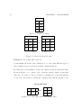
After flipping the top triangle . . . . . . . . . . . . . . . . . . . . . .
After drawing a new triangle . . . . . . . . . . . . . . . . . . . . . . .
After changing the filling pattern of the bottom triangle . . . . . . .
After changing the border width of the bottom triangle . . . . . . . .
Popup error message 1 . . . . . . . . . . . . . . . . . . . . . . . . . .
Popup error message 2 . . . . . . . . . . . . . . . . . . . . . . . . . .
Adding a line to the graph . . . . . . . . . . . . . . . . . . . . . . . .
Adding a box to the graph . . . . . . . . . . . . . . . . . . . . . . . .
Popup warning message . . . . . . . . . . . . . . . . . . . . . . . . .
44
45
46
46
47
48
49
49
50
51
52
53
54
56
56
56
58
58
59
60
60
60
61
62
62
5.1
5.2
5.3
5.4
5.5
5.6
5.7
5.8
5.9
5.10
5.11
5.12
5.13
5.14
5.15
System Architecture . . . . . . . . . . . . . . . . . . . . . . . . . . .
Syntax Tree for “NewText <- display2D ( ) Text; ” . . . . . . . . . .
Syntax Tree for “NewText2 <- display2D (TextVocabulary) Text2; ”
Multiple text strings in the relation Picture . . . . . . . . . . . . . .
Displaying multiple text . . . . . . . . . . . . . . . . . . . . . . . . .
Nested relation Graph and its underlying dot relations . . . . . . . .
A tree structure representation for the nested relation Graph . . . . .
Algorithm for the function dispNestedRel . . . . . . . . . . . . . . . .
An open polyline . . . . . . . . . . . . . . . . . . . . . . . . . . . . .
Algorithm for the function run() in detectFileDiffThread.java . . . .
Xfig File for a Polyline . . . . . . . . . . . . . . . . . . . . . . . . . .
A sample original Xfig file representing non-polylines . . . . . . . . .
A sample updated Xfig file representing non-polylines . . . . . . . . .
An algorithm for detecting violations to Rule #2 . . . . . . . . . . .
Xfig file for three points . . . . . . . . . . . . . . . . . . . . . . . . .
64
66
66
73
73
76
76
78
80
83
84
85
86
87
89
6.1
6.2
Relation UpdatedPoints3 . . . . . . . . . . . . . . . . . . . . . . . . .
Polymorphic relation UpdatedPoints3 . . . . . . . . . . . . . . . . . .
98
98
LIST OF FIGURES
6.3
6.4
ix
jRelix input for displaying the matrix form of the relation Chair . . . 101
Matrix form of the relation Chair . . . . . . . . . . . . . . . . . . . . 101
List of Tables
2.1
2.2
2.3
The display form of the nested relation Graph . . . . . . . . . . . . .
µ-join operators . . . . . . . . . . . . . . . . . . . . . . . . . . . . . .
σ-join operators . . . . . . . . . . . . . . . . . . . . . . . . . . . . . .
17
24
25
3.1
3.2
3.3
3.4
Xfig file header . . . . . . .
Type 2 Xfig Object Format
Type 4 Xfig Object Format
Type 6 Xfig Object Format
.
.
.
.
.
.
.
.
.
.
.
.
.
.
.
.
.
.
.
.
.
.
.
.
.
.
.
.
.
.
.
.
.
.
.
.
.
.
.
.
.
.
.
.
.
.
.
.
.
.
.
.
.
.
.
.
.
.
.
.
.
.
.
.
.
.
.
.
.
.
.
.
.
.
.
.
29
31
33
34
4.1
4.2
4.3
4.4
4.5
4.6
4.7
4.8
4.9
4.10
4.11
4.12
4.13
4.14
4.15
Relation Text . . . . . . . . . . . . .
Relation Points . . . . . . . . . . . .
Relation LabelledPoints . . . . . . .
Relation Lines . . . . . . . . . . . . .
Relation LabelledLines . . . . . . . .
Relation Triangle . . . . . . . . . . .
Relation LabelledTriangle . . . . . .
Relation Polyline . . . . . . . . . . .
Relation LabelledVertexPolyline . . .
Relation NestedPolyline . . . . . . .
Nested relation Graph . . . . . . . .
Relation Text2 . . . . . . . . . . . .
Relation TextVocabulary . . . . . . .
Relation NewTriangle . . . . . . . . .
Relation NewTriangle (after update)
.
.
.
.
.
.
.
.
.
.
.
.
.
.
.
.
.
.
.
.
.
.
.
.
.
.
.
.
.
.
.
.
.
.
.
.
.
.
.
.
.
.
.
.
.
.
.
.
.
.
.
.
.
.
.
.
.
.
.
.
.
.
.
.
.
.
.
.
.
.
.
.
.
.
.
.
.
.
.
.
.
.
.
.
.
.
.
.
.
.
.
.
.
.
.
.
.
.
.
.
.
.
.
.
.
.
.
.
.
.
.
.
.
.
.
.
.
.
.
.
.
.
.
.
.
.
.
.
.
.
.
.
.
.
.
.
.
.
.
.
.
.
.
.
.
.
.
.
.
.
.
.
.
.
.
.
.
.
.
.
.
.
.
.
.
.
.
.
.
.
.
.
.
.
.
.
.
.
.
.
.
.
.
.
.
.
.
.
.
.
.
.
.
.
.
.
.
.
.
.
.
.
.
.
.
.
.
.
.
.
.
.
.
.
.
.
.
.
.
.
.
.
.
.
.
.
.
.
.
.
.
.
.
.
.
.
.
.
.
.
.
.
.
.
.
.
.
.
.
.
.
.
.
.
.
.
.
.
.
.
.
.
.
.
.
.
.
.
.
.
36
38
39
41
42
44
45
47
48
50
52
55
55
57
61
5.1
5.2
5.3
5.4
Relation NestedPoints .
Relation NestedLines . .
Relation NestedTriangles
A relation represented by
. . . . .
. . . . .
. . . . .
the Xfig
. . .
. . .
. . .
from
. . . .
. . . .
. . . .
5.15 .
.
.
.
.
.
.
.
.
.
.
.
.
.
.
.
.
.
.
.
.
.
.
.
.
.
.
.
.
80
81
82
90
6.1
6.2
6.3
6.4
6.5
A vocabulary relation
Spline types . . . . .
A vocabulary relation
A vocabulary relation
A vocabulary relation
ellipses and circles . . . . .
. . . . . . . . . . . . . . . .
splines . . . . . . . . . . . .
arcs . . . . . . . . . . . . .
the polar coordinate system
.
.
.
.
.
.
.
.
.
.
.
.
.
.
.
.
.
.
.
.
.
.
.
.
.
.
.
.
.
.
.
.
.
.
.
93
94
94
94
95
for
. .
for
for
for
.
.
.
.
.
.
.
.
.
.
.
.
x
.
.
.
.
. .
. .
. .
file
. . . .
. . . .
. . . .
Figure
.
.
.
.
.
.
.
.
.
.
LIST OF TABLES
6.6
6.7
6.8
6.9
6.10
A vocabulary relation for
Relation LabelledPoints2
Relation Points3 . . . .
Relation Chair . . . . .
Relation ChairVocab . .
xi
cart1show
. . . . . .
. . . . . .
. . . . . .
. . . . . .
and cart2show
. . . . . . . . .
. . . . . . . . .
. . . . . . . . .
. . . . . . . . .
.
.
.
.
.
.
.
.
.
.
.
.
.
.
.
.
.
.
.
.
.
.
.
.
.
.
.
.
.
.
.
.
.
.
.
.
.
.
.
.
.
.
.
.
.
. 96
. 96
. 98
. 100
. 100
A.1 Keywords in vocabulary relations for display2D . . . . . . . . . . . . 105
A.2 Xfig object parameter names and the keywords for display2D . . . . . 106
Chapter 1
Introduction
Visualization is the process of transforming data, information, and knowledge into
visual form making use of humans’ natural visual capabilities [GEC98]. It significantly improves our understanding of complicated relations and larger quantities of
data.
This thesis presents the design and implementation of a two-dimensional display
editor, which graphically visualizes the data stored in relations, for a relational database programming system jRelix [Bak98, He97, Hao98, Sun00, Yua98].
In this chapter, we will introduce the background and preliminary material needed
throughout the thesis. Section 1.1, describes the research background and the previous achievements in the area of information visualization. Section 1.2 reviews the
relational data model. Section 1.3 presents the motivation for the integration of information visualization into JRelix. The last section serves as an outline of the topics
covered in this thesis.
1.1
Information Visualization
Information visualization is defined as “the use of computer-supported, interactive, visual representations of abstract nonphysically based data to amplify cognition” [CMS99].
It is a broad and complex research area, which involves research in visual design,
1
2
CHAPTER 1. INTRODUCTION
human-computer interaction, computer graphics, database systems and cognitive science. The two main aspects of the research are static and interactive information visualization. For static information visualization, researchers focus on methods to display
different types of data statically, such as scientific numerical data, relational data and
geographical data. For interactive information visualization, researchers focus on realtime interactive visualization, which is the “ability of the system to respond quickly
to the users’ direct manipulation commands” [CC96]. Dynamic queries [AWS92] is
one of the major themes for interactive information visualization.
1.1.1
Static Information Visualization
According to the data type taxonomy [Shn96] proposed by Shneiderman, static information visualization is used to visualize seven data types: one-dimensional, twodimensional, three-dimensional, temporal, multi-dimensional, tree and network data.
One-Dimensional Data
One-dimensional data is linear data, such as text, which includes pure text documents,
source code of computer programs, etc. Naturally, a user can easily visualize a small
one-dimensional data set, such as a short letter. To enable users to visualize the
overall structure of a very long textual document and to understand the connections
between parts of the document quickly, special techniques have to be applied.
Through the work of many researchers, there have been several tools created for
visualizing large one-dimensional data sets. Developed in AT&T Bell Laboratories,
the Seesoft software visualization system [ESJ92] can display and analyze up to 50000
lines of source code. Each line in the source code is visualized as a single coloured
thin line. The line colour can represent various aspects, including the date that a
line is created, the date that a line is modified, etc. Each file is represented by a
rectangle, grouping all of the lines in the file. The actual code can be displayed in
an additional window. The reduced representation of the source code provides users
with an entire overview of a large software program. It also allows users to accomplish
1.1. INFORMATION VISUALIZATION
3
version control efficiently [ESJ92]. Another approach to visualizing one-dimensional
data is Document Lens [RM93]. It visualizes multiple pages of text in a reduced size
using a three-dimensional fisheye view [Fur81]. This allows users to access parts of a
presentation quickly without losing the global context.
Two-Dimensional Data
Two-dimensional data consists of two attributes. In a vector format, two-dimensional
data is stored in terms of x and y coordinates. Geographic information systems (GIS)
is the most common research area in two-dimensional data visualization. GIS is a tool
for storing and retrieving, transforming and displaying spatial data [Bur86]. A GIS
is usually a combination of a collection of map layers which can be linked together.
Each layer is a two-dimensional representation for an aspect, such as, cities, rivers,
mountains, roads, etc.
One approach for displaying the map layers, presented by Egenhofer and Richards,
is to use a combination of data cubes and map templates [ER93]. The data cubes
represent the geographic data. Each cube has a spatial location and orientation. The
map templates describe the display parameters, which are rules for displaying data
cubes among different views.
Another effort to visualize GIS is Geditor [Che01], a GIS editor and visualizer
for a relational database system, jRelix (see section 1.2.2). The Geditor analyzes
both spatial and non-spatial data stored in the relational database, and displays map
layers in a graphical user interface written in Java Foundation Classes (JFC) Swing.
The Geditor allows users to edit maps, generate thematic maps and perform spatial
queries [Che01].
In addition to geographic information, two-dimensional relations can also be categorized as two-dimensional data. To visualize this relational information by graphical
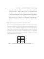
presentations, such as bar charts, scatter plots, connected graphs, etc, a linear model
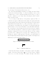
for generating graphical visualization [Mac86], shown in Figure 1.1 is usually used.
4
CHAPTER 1. INTRODUCTION
Presentation Tool
Application
Database
Relations
Data
extract
Graphical design
synthesize
Image
render
Figure 1.1: A linear model for generating a graphical visualization from relational
data
Three-Dimensional Data
For scientific data visualization, such as architectural and medical applications, twodimensional images can not always provide a comprehensive mapping from the data
to the graphical presentation. Therefore, it is better to use three-dimensional data
visualization.
For example, the Visible Human Project [NSP96] created a collection of detailed,
three-dimensional representations of the human body. Through a user interface in
the National Library of Medicine, users can visualize the collection, browse contents
and retrieve images.
Another example is WebBook [CRY96], a three-dimensional representation for
HTML Web pages. Each page of WebBook is a page from the web. A collection of
web pages is visualized as a simulated three-dimensional physical book. WebBook
users can quickly interact with each page and find the connections between the pages
of the book.
Multi-dimensional Data
Multi-dimensional data consists of more than three attributes. Most relational and
statistical databases are considered to be multi-dimensional data.
The parallel coordinate system [Ins81], proposed by Inselberg, is an effective technique to present multi-dimensional data. It maps higher dimensional data sets into
two-dimensions. For Cartesian coordinates, all axes are perpendicular. Therefore,
1.1. INFORMATION VISUALIZATION
5
having more than three orthogonal axis is impossible in three-dimensions. In the
parallel coordinate system, the axes are represented by parallel and equally spaced
straight lines in a plane. Several multi-dimensional geometric shapes, such as points,
lines, etc., can be displayed by using the parallel coordinates. The parallel coordinate
system can be found in applications for air traffic control, robotics, computer vision,
computational geometry, statistics and instrumentation [Ins90].
There are many other interesting approaches to multi-dimensional data visualization. For example, there is Table Lens [RC94], a spreadsheet-like tool for visualizing
a table, much larger than the tables supported by conventional spreadsheets. Table
Lens displays a table by using the focus+context (fisheye) mechanism, which allows
users to see the global graphical presentation of the table and to zoom in on specific table cells. There is also the HomeFinder [WS92], an application allowing users
to do dynamic database searches to provide multi-dimensional real-estate data visualizations. Additionally, a commercial software product called Spotfire provides
multi-dimensional data visualization for various areas, such as life science, engineering, finance, etc. It is also a system based on the concept of interactive dynamic
queries. Its users can interactively query, filter, zoom, and pan visualizations [Ahl96].
Temporal Data
Temporal data is data that explicitly refers to time. Project time lines and historical
data are both temporal data.
LifeLines [PMR+ 96], developed at the University of Maryland, is an application
providing a personal history visualization. On one screen, an individual’s information
such as criminal record, medical, employment and education history, is displayed as
horizontal lines labelled with detailed information. The flexible time scale for the
display could be in years, months, weeks, days, hours and even in minutes.
For many video and animation editing software packages, such as Adobe Premiere [Ado06], Macromedia Director [Mac04] and Flash [Mac05], temporal data visualization is used to synchronize layers and objects.
6
CHAPTER 1. INTRODUCTION
Tree (Hierarchical) Data
In graph theory, a tree is a collection of nodes with each node having a link to one parent node (except the root node). Business organizations, family trees, animal species
trees and directories of a computer hard disk can all be organized in a hierarchical
tree structure.
One approach to visualizing tree data is the Cone/Cam Tree [RMC91], an animated three-dimensional visualization of hierarchical structures. The Cone Tree is
a vertically oriented tree structure of vertical cone shapes with the parent nodes at
the cone tips. Child nodes are spaced equally in the base of a (vertical) cone shape
with the parent node (at the top). The Cam Tree is a horizontally oriented tree
structure of horizontal cone shapes with the parent node at the cone tips. Child
nodes are spaced equally in the base of a (horizontal) cone shape with the parent
node (at the left). When the user selects a node with the mouse, the selected node is
highlighted and the Cone/Cam Tree rotates to bring the selected node to the front
of the view. This interactive animation shifts some of the user’s cognitive load to the
human perceptual system. Also the user gains insight into the relationships between
substructures [RMC91].
Another approach for the hierarchical information visualization is a Tree-Map,
which is a one hundred-percent utilized rectangular display filled with nested rectangles [JS91]. To represent a tree by a Tree-Map, each node of the tree must have an
attribute representing its size or weight. Each leaf node of the tree is represented by
a rectangle. The size of a rectangle in the Tree-Map indicates the relative size within
the entire hierarchy. The contents of a node, such as name and size, can be displayed
in the rectangle representing the node. The application of the Tree-Map is broad. It
can be used to give a better representation of the utilization of storage space on a
hard disk. It can also visualize the number of book collections by subject in a library,
or the number of employees and the amount of budget allocated to each department
in a business organization [Shn92].
1.1. INFORMATION VISUALIZATION
7
Network Data
Network data refers to objects linked to an arbitrary number of other objects. Since
there can be multiple paths between two objects (nodes), a network can be very complicated. Therefore, network data visualization is an essential tool for understanding
the network structure.
Becker, Eickt, and Wilks [BEW95] proposed three techniques, linkmap, nodemap
and matrix display, to visualize an American network of telecommunication traffic
on a geographical map. The linkmap technique works as follows. On a map, according to the geographical relationship of two nodes, a coloured line is drawn to
connect the nodes. However, there may be too many links causing a map-clutter
problem. Therefore, an alternative approach to visualize the network is presented.
The nodemap displays node data by showing a symbol, such as a circle or a square
at each node on the map, with an aggregation of node information. The nodemap
solves the display clutter problem, but it loses detailed information about particular
links. Like linkmap, the matrix display concentrates on the links of a network. It
uses a visual prominence for longer line links. The longer (transcontinental) linkage
lines may overplot other lines. Matrix display gives a better graphical presentation
than linkmap when there are many lines on the display map [BEW95].
Three-dimensional visualization is mostly used for network data. Various visualizations are developed to show the World Wide Web. The Natto View [SM97] is an
interactive visualization tool for a collection of web pages. Each web page is a node
placed on a flat horizontal plane, which has two axes for representing two attributes
of a web page. The attribute can be a page name, file size, number of links, number
of images, etc. The position of the node is determined by the value of the two attributes of the corresponding web page. A user can select a node and lift it up. By
doing so, the links of the selected node are raised, so that the user sees a dynamic
three-dimensional display. An alternative approach is a three-dimensional hyperbolic
space, which is formed inside a sphere. Each node represents a web page and is placed
inside the sphere and connected to other nodes by Euclidean straight lines [MB95].
8
CHAPTER 1. INTRODUCTION
1.1.2
Interactive Information Visualization
Dynamic Queries
As the main approach for interactive information visualization, dynamic queries [AWS92]
allow users to formulate queries with graphical widgets, such as buttons, check boxes
or sliders, and visualize results immediately. For example, when the user is moving the
drag box in a slider, the value for the corresponding criterion changes, and simultaneously the user sees that the visualization is changing too. Compared to Structured
Query Language (SQL), dynamic queries do not require users to have knowledge of
the syntax or semantics of query commands. The graphical presentation of the database and the immediate graphical feedback for dynamic queries provides users with
a better understanding of the database and query results.
As mentioned before, the commercial application, Spotfire [Ahl96] is a system
based on the concept of dynamic queries. There is also the HomeFinder [WS92], an
application visualizing multi-dimensional real-estate data. The HomeFinder displays
a map containing all of the locations of houses for sale. By manipulating sliders, users
can perform dynamic database queries by selecting the home’s distance to desired
locations, the numbers of bedrooms and the cost of the house. As these selections are
changed, the houses that best satisfy the criteria are immediately displayed.
Another tool, called PDQ (Pruning with Dynamic Queries) Tree-browser [KPS97],
is used for hierarchical data visualization with dynamic queries. PDQ Tree-browser
provides a graphical overview and detailed view of a tree in node-link forms. A
dynamic query panel, consisting of an attributes list on the left and a widgets panel
on the right, is below the tree display. Dynamic queries can be done at different levels
of the tree. The result nodes matching the query are highlighted.
1.2. RELATIONAL DATABASE SYSTEM
1.2
9
Relational Database System
1.2.1
Relational Model
The relational model of data was invented by Codd [Cod70]. Since then, it has been
recognized for its simplicity, uniformity, data independence, integrity and evolvability [Ger75]. In his relational model, a new data structure, called a relation, which is
represented in a table format, is used to model and store data. Each row in the table
is called a tuple. Each column is referred to as a domain. The name of a domain is
an attribute. From a mathematical perspective, a relation is a subset of the Cartesian
product of its domains. Each relational table has the following properties:
1. All rows are distinct from each other.
2. The ordering of rows is immaterial.
3. Each column has a different name (attribute) and the ordering of columns is
immaterial.
4. The value in each row under a given column is atomic, i.e., it is non-decomposable.
Operations on Relations
Operations on relations are performed by relational algebra, which is proposed by
Codd [Cod70]. In relational algebra, the relational operators take relations as operands
and return a new relation as the result. Depending on the number of operands, the
relational algebra operations are classified as unary or binary operations. Unary operators require one relation as the lone operand. Projection and selection operations
are both unary. Binary operators take two relations as operands. µ-join and σ-join
are binary operations.
Operations on Domains
The algebra on attributes is called domain algebra. Proposed by Merrett [Mer84],
domain algebra treats attributes independently from relations. It allows users to
10
CHAPTER 1. INTRODUCTION
create new domains from existing ones, and also to generate new values from existing
values in a tuple or from values along an attribute. The domain algebra consists of
horizontal and vertical operations.
• Horizontal operations
– Constant
– Rename
– Function
– If-then-else
• Vertical operations
– Reduction
– Equivalence Reduction
– Functional Mapping
– Partial Functional Mapping
1.2.2
jRelix
jRelix (the java implementation of a Relational database programming language in
Unix) was developed in the Aldat lab of the School of Computer Science at McGill
University. jRelix contains a database management system (DBMS) and a programming language Aldat (Algebraic Data Language), which supports relational algebra and domain algebra on flat and nested relations [Hao98, Yua98, Sun00, Kan01,
Cha02]. The integration of computations (procedures and functions) [Bak98] and
ADT (Abstract Data Type) [Zhe02] to jRelix provides procedural abstraction and
data abstraction. A GIS editor (Geditor) [Che01] in jRelix, allows users to view graphical maps and provides a set of GIS functions. jRelix aldatp (aldat protocol) [Wan02]
integrates collaborative and distributed Internet capability into jRelix.
1.3. MOTIVATION
1.3
11
Motivation
The graphical representation of information is referred to as information graphics.
The basic objects forming an information graphic are text, points, lines, boxes, arcs,
and circles. The basic elements used to describe the properties of information graphics
are colour, texture and scale. For example, LiftLines [PMR+ 96] uses coloured lines,
text, and coloured rectangles to record an individual’s history. HomeFinder [WS92]
uses coloured points, a textured area and text to represent the information on houses
for sale. Cone/Cam Tree [RMC91] uses ellipses (two arcs) to represent the projection
of the bases of three-dimensional cones on to a two-dimensional textured plane.
jRelix, as a high-level database programming and query language, is proposed to
provide applications in various areas, such as expert systems, numerical computing,
data mining, information visualization, etc. In order to enable jRelix to visualize
information, it is necessary to implement the mechanism for the drawing of basic
graphical objects.
Static graphical representation of information has improved our understanding and
recognition of complex data sets. But our ability to understand graphical information can be even better with user interactivity in visualizations. For example, with
Cone/Cam Tree [RMC91] users can select a node and the whole Cone/Cam Tree rotates to bring the selected node to the front of the view. In Natto View [SM97] users
can select a node lying in a two-dimensional plane and lift it up. Then all of the links
to the selected node are raised simultaneously. All of these techniques give users insight into the visualizations. However, users are limited to manipulating the existing
structure without operations such as creation, deletion, relocation or modification.
We propose to give jRelix an extensive ability for interactive information visualization. In other words, jRelix will not only provide information graphics, but will
also allow users to operate on the visualizations interactively . We need to develop
an automatic mechanism that analyzes user changes to visual content and makes
updates to the database accordingly.
12
1.4
CHAPTER 1. INTRODUCTION
Thesis Outline
The current chapter, chapter 1, presented a literature background on information
visualization, relational models and jRelix. In addition, the motivation and outline of
this thesis are presented in this chapter. Chapter 2 introduces the use of the jRelix
system. Chapter 3 gives a tutorial of Xfig and the Xfig file format. Chapter 4 is the
user manual on display2D. Chapter 5 presents the implementation of the display2D
operation in jRelix. Chapter 6 concludes the thesis with a summary and proposes
future work.
Chapter 2
Overview of jRelix
In this chapter, we give a tutorial about the current jRelix system, so that the reader
can understand material presented in the later chapters of this thesis. Section 2.1
explains how to declare domains and relations in jRelix. Section 2.2 introduces
relational algebra, including assignments, unary and binary relation operations.
2.1
2.1.1
Declarations
Domain Declarations
A relation is defined on one or more attributes. Each attribute is associated with a
set of values called a domain [Mer99]. The data type of an attribute is determined
by its domain. In jRelix, there are two types of domain declarations, atomic-typed
and complex-typed.
JRelix provides eleven atomic data types: integer, short, long, float, double,
boolean, string, text, numeric, universal [Mer01] and attribute [Mer01]. The syntax
for the atomic-typed domain declaration is the following:
domain <dom name1, dom name2, ...> <atomic data type>;
A nested relation is one that can contain another relation as its attributes. A
complex-typed domain declaration declares nested domains from nested relations.
13
14
CHAPTER 2. OVERVIEW OF JRELIX
This allows multiple level nesting in jRelix. The syntax for the complex-typed domain
declaration is the following:
domain <nested domain name> ( <dom name1, dom name2, ...> );
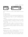
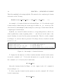
An example of a domain declaration is shown in Figure 2.1. Note that the nested
domain Lines is defined using the atomic-typed domains, x1, y1, x2 and y2. The
2-level nested domain Graph is defined using the atomic-type domain label and the
complex-typed domain Lines.
In jRelix, once a nested domain is declared, a corresponding relation, called a dot
relation (which has a name beginning with a “.” and followed by the name of the
nested domain), is created by the system automatically. Therefore, in the example
from Figure 2.1, relation .Lines is generated. We will provide more details about this
in section 2.1.2.
>domain
>domain
>domain
>domain
x1, y1, x2, y2 intg;
label strg;
Lines (x1, y1, x2, y2);
Graph (label, Lines);
<<
<<
<<
<<
integer type domain >>
string type domain >>
nested domain >>
nested domain with 2-level nesting>>
Figure 2.1: An example of domain declaration
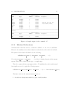
To display the information for all the domains currently declared in the system,
we use the command “sd;”. To show the information for a specific domain, we use
the command “sd ” followed by the domain name.
sd <dom name>;
Given the domains declared in Figure 2.1, the output for the “sd” command is
shown in Figure 2.2.
To delete a specific domain from the system, we use the command “dd” followed
by the domain name.
dd <dom name>;
2.1. DECLARATIONS
15
>sd;
------------------------------- Domain Entry ------------------------------Name
Type
NumRef
IsState
Dom_List
---------------------------------------------------------------------------y2
integer
1
false
y1
integer
1
false
Lines
idlist
1
false
.id, x1, y1, x2, y2,
Graph
idlist
0
false
.id, label, Lines,
label
string
1
false
x2
integer
1
false
x1
integer
1
false
--------------------------------------------------------------------------->sd x1;
------------------------------- Domain Entry ------------------------------Name
Type
NumRef
IsState
Dom_List
---------------------------------------------------------------------------x1
integer
1
false
----------------------------------------------------------------------------
Figure 2.2: Sample output for the command “sd”
2.1.2
Relation Declarations
As mentioned in the last section, a relation is defined on one or more attributes.
Therefore the attributes in a relation must be declared before the relation is declared.
The syntax of the relation declaration is the following:
relation <rel name> ( <dom name1, dom name2, ...> );
Note that <dom name1, dom name2, ...> is a list of existing domains in the current
system. They can be either atomic type or complex type.
The above syntax declares an empty relation. To initialize the relation with actual
data tuples, we need to apply the following syntax:
relation <rel name>(<dom name1, dom name2, ...>) <- <Initialization list>;
The three rules for the initialization list are:
1. A relation is always surrounded by a pair of curly brackets.
16
CHAPTER 2. OVERVIEW OF JRELIX
2. Inside a relation, each tuple is surrounded by a pair of round brackets.
3. Tuples are separated by commas.
Figure 2.3 gives an example of a flat relation declaration. In addition, after any
relation is initialized, in the directory where jRelix is running, a file having the same
name as the relation and containing the data of the relation is created by the jRelix
system. Given the relation Points from Figure 2.3, the content of the file “Points”
is shown in Figure 2.4.
relation Points(x1, y1) <- {
(1363, 3013),
(2942, 3010),
(3426, 1508),
(2148, 583),
(873, 1514)};
Figure 2.3: Declare the flat relation Points
873^F1514^F
1363^F3013^F
2148^F583^F
2942^F3010^F
3426^F1508^F
Figure 2.4: Content of the file Points
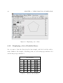
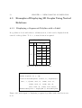
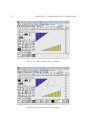
Either syntax could also be followed to declare and initialize a nested relation.
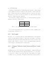
Table 2.1 shows the nested relation Graph. Its declaration and initialization are
shown in Figure 2.5.
Only the very top level relation (e.g. Graph) is initialized during a nested relation
declaration. However, as mentioned in the last section 2.1.1, once a nested domain
is declared, a corresponding invisible relation, which has a name beginning with a “.”
is created. In this example, relation .Lines is created.
2.1. DECLARATIONS
17
Graph
label
group1
group2
Lines
x1
y1
x2
y2
2000
1000
3000
1000
5000
3000
1000
2000
1500
500
10000
3000
2000
2000
1500
3000
Table 2.1: The display form of the nested relation Graph
relation Graph (label, Lines) <("group1", { (2000, 1000, 3000,
(5000, 3000, 1000,
("group2", { (1500, 500, 10000,
(2000, 2000, 1500,
};
{
1000),
2000) }),
3000),
3000) })
Figure 2.5: Declare the nested relation Graph
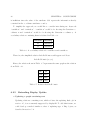
To reveal the data stored in any relation, we use the command “pr”. In Figure 2.6,
the contents of the relation Graph and its underlying dot relation .Lines are printed.
The top level relation, Graph, and its underlying dot relation(s) .Lines, are linked
by surrogate numbers. In the top level relation, the surrogate numbers are stored in
the nested attributes. In the dot relations, the attribute .id contains the surrogate
numbers linking the current dot relation to its corresponding upper level relation.
Note that all dot relations have the attribute .id. In our example, the nested attribute
Lines in the relation Graph has surrogates 1 and 2 stored. In the relation .Lines,
attribute .id has value 1 and 2. Therefore, the first two tuples in the relation .Lines
can be linked to the first tuple of the relation Graph by surrogate 1. The last two
tuples in the relation .Lines can be linked to the last tuple of the relation Graph by
surrogate 2.
Besides the command “pr”, there are two additional commands for performing
operations on declared relations. To remove a specific relation from the system, we
use command “dr”.
18
CHAPTER 2. OVERVIEW OF JRELIX
>pr Graph;
+----------------------+----------------------+
| label
| Lines
|
+----------------------+----------------------+
| group1
| 1
|
| group2
| 2
|
+----------------------+----------------------+
relation Graph has 2 tuples
>pr .Lines;
+----------------------+-------------+-------------+-------------+-------------+
| .id
| x1
| y1
| x2
| y2
|
+----------------------+-------------+-------------+-------------+-------------+
| 1
| 2000
| 1000
| 3000
| 1000
|
| 1
| 5000
| 3000
| 1000
| 2000
|
| 2
| 1500
| 500
| 10000
| 3000
|
| 2
| 2000
| 2000
| 1500
| 3000
|
+----------------------+-------------+-------------+-------------+-------------+
relation .Lines has 4 tuples
Figure 2.6: The nested relation Graph and its underlying dot relation .Lines
dr <rel name>;
To list all the declared relations in the current system, the command “sr;” should be
used. To get the information of a specific relation, we do the following:
sr <rel name>;
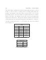
A sample output for the command “sr” is shown in Figure 2.7.
2.2
2.2.1
Relational Algebra
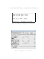
Assignments
The assignment operator is used to create new relations from old ones. There are two
types of assignment in jRelix, replacement assignment and incremental assignment.
The replacement assignment copies the right-hand operand to the left-hand operand.
The syntax for the replacement assignment is the following:
2.2. RELATIONAL ALGEBRA
19
>sr;
------------------------------ Relation Table -----------------------------Name
Type
Arity
NTuples
Sort
Active
---------------------------------------------------------------------------Graph
relation
2
2
2
0
Points
relation
2
5
2
0
--------------------------------------------------------------------------->sr Points;
------------------------------ Relation Entry -----------------------------Name
Type
Arity
NTuples
Sort
Active
---------------------------------------------------------------------------Points
relation
2
5
2
0
----------------------------------------------------------------------------
Figure 2.7: Sample output for the command “sr”
<new relname> <- <expression>;
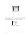
or:
<rel L> [<attr list rel L> <- <attr list rel R>] <rel R>;
The syntax for the incremental assignment is the following:
<new relname> <+ <expression>;
or:
<rel L> [<attr list rel L> <+ <attr list rel R>] <rel R>;
The incremental assignment appends the additional tuples from the right-hand
relation to the left-hand relation. The attributes in left-hand relation must be compatible with those in the right-hand relation. Figure 2.8 gives examples of assignment
operations.
2.2.2
Unary Operations
Unary operations take a single relation as input and generate a new relation as output.
jRelix provides three unary operations, projection, selection and T-selection.
• Projection
20
CHAPTER 2. OVERVIEW OF JRELIX
>domain x1, y1, x2, y2 intg;
>relation Points1(x1, y1) <- {(1000, 2000), (1000, 4000)};
>NewPoints <- Points1;
>pr NewPoints;
+-------------+-------------+
| x1
| y1
|
+-------------+-------------+
| 1000
| 2000
|
| 1000
| 4000
|
+-------------+-------------+
relation NewPoints has 2 tuples
>relation Points2(x1, y1)<-{(5000, 6000)};
>NewPoints <+ Points2;
>pr NewPoints;
+-------------+-------------+
| x1
| y1
|
+-------------+-------------+
| 1000
| 2000
|
| 1000
| 4000
|
| 5000
| 6000
|
+-------------+-------------+
relation NewPoints has 3 tuples
>Points2 [y1, x1 <+ x1, y1] NewPoints;
>pr Points2;
+-------------+-------------+
| x1
| y1
|
+-------------+-------------+
| 2000
| 1000
|
| 4000
| 1000
|
| 5000
| 6000
|
| 6000
| 5000
|
+-------------+-------------+
relation Points2 has 4 tuples
Figure 2.8: Assignment operations
2.2. RELATIONAL ALGEBRA
21
The syntax for the projection operation is the following:
[<dom name1, dom name2, ...>] in <source rel>;
The projection operation extracts a subset of a source relation (source rel)
based on a list of specified attributes (dom name1, dom name2, ...). Duplicate tuples are removed from the result relation. An example of a projection
operation is shown in Figure 2.9.
>pr Points1;
+-------------+-------------+
| x1
| y1
|
+-------------+-------------+
| 1000
| 2000
|
| 1000
| 4000
|
+-------------+-------------+
relation Points1 has 2 tuples
>pr [x1] in Points1;
+-------------+
| x1
|
+-------------+
| 1000
|
+-------------+
expression has 1 tuple
Figure 2.9: Example of a projection operation
• Selection
The syntax for the selection operation is the following:
where <selection condition> in <source rel>;
This operation selects a set of tuples from a source relation (source rel) according to a boolean condition (selection condition). Each tuple in the source
relation is evaluated by the boolean condition. Only those tuples that evaluate
to true will be selected. The resulting relation has the same attributes as the
source relation. An example of the selection operation is shown in Figure 2.10.
22
CHAPTER 2. OVERVIEW OF JRELIX
>pr Points1;
+-------------+-------------+
| x1
| y1
|
+-------------+-------------+
| 1000
| 2000
|
| 1000
| 4000
|
+-------------+-------------+
relation Points1 has 2 tuples
>pr where y1>2005 in Points1;
+-------------+-------------+
| x1
| y1
|
+-------------+-------------+
| 1000
| 4000
|
+-------------+-------------+
expression has 1 tuple
Figure 2.10: Example of a selection operation
• T-selection
The syntax for the T-selection operation is the following:
[<dom name1, dom name2, ...>] where <selection condition> in <source rel>;
T-selection is a combination of projection and selection. The selection is done
first, then the projection. Figure 2.11 gives an example of T-selection operation.
2.2.3
Binary Operations
The binary operations of relational algebra are extensions of the binary operations
on sets [Mer84]. Binary operations take two relations as input and generate a new
relation as output. jRelix provides two categories of binary operations, µ-join and
σ-join. The syntax for join operations is as follows:
<expression> JoinOperator <expression>;
or:
<expression> [<attr list> : JoinOperator :
<attr list>] <expression>;
2.2. RELATIONAL ALGEBRA
23
>pr Points1;
+-------------+-------------+
| x1
| y1
|
+-------------+-------------+
| 1000
| 2000
|
| 1000
| 4000
|
+-------------+-------------+
relation Points1 has 2 tuples
>pr [x1] where y1>2005 in Points1;
+-------------+
| x1
|
+-------------+
| 1000
|
+-------------+
expression has 1 tuple
Figure 2.11: Example of a T-selection operation
In the first syntax, the two operands join on their common attributes. If the two
operands do not have any common attributes, the second syntax should be used to
specify the joining attributes (attr list).
• µ-joins
µ-joins correspond to the binary set operations including union, intersection
and difference. In general, µ-joins consist of three parts, left, center and right.
Given two relations R(X, Y) and S(Y, Z) sharing a common attribute set, Y,
we have:
center = {(x, y, z ) | (x, y) ∈ R and (y, z ) ∈ S }
left = {(x, y, DC) | (x, y) ∈ R and ∀ z (y, z ) 6∈ S }
right = {(DC, y, z ) | (y, z ) ∈ S and ∀ x (x, y) 6∈ R}
Given two relations R(W, X) and S(Y, Z) sharing no common attribute set, we
have:
center = {(w, x, y, z ) | (w, x ) ∈ R and (y, z ) ∈ S and x = y }
left = {(w, x, y, DC) | (w, x ) ∈ R and x = y ⇒ ∀ z (y, z ) 6∈ S }
24
CHAPTER 2. OVERVIEW OF JRELIX
right = {(DC, x, y, z ) | (y, z ) ∈ S and x = y ⇒ ∀ x (w, x ) 6∈ R}
Note that the symbol DC stands for don’t care, a null value defined in jRelix.
The complete list of µ-join operators is shown in Table 2.2. Figure 2.12 gives
an example of a µ-join operation.
Name
Operator
Definition
Intersection join
ijoin
center
Union join
ujoin
left ∪ center ∪ right
Left join
ljoin
left ∪ center
Right join
rjoin
center ∪ right
Left difference join
djoin
left
Right difference join
drjoin
right
Symmetric difference join
sjoin
left ∪ right
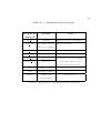
Table 2.2: µ-join operators
• σ-joins
The σ-joins extend the truth-valued comparison operations on sets to relations
by applying them to each set of values of the join attribute for each of the
other values in the two relations [Mer84]. We define the σ-joins using the
following notations. In relation R(W, X) and S(Y, Z), Rw is the set of values
of X associated by R with a given value, w, of W, and Sz is the set of values of
Y associated by S with a given value , z, of Z. If W and X are disjoint sets of
attributes of R, and Y and Z are disjoint sets of attributes of S, the following
definitions shown in Table 2.3 are held. Note that X and Y could be the same
set of attributes, but at the very least they must be compatible attribute sets.
Figure 2.13 gives an example of σ-join operations.
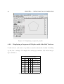
2.2. RELATIONAL ALGEBRA
25
>pr Points1;
+-------------+-------------+
| x1
| y1
|
+-------------+-------------+
| 1000
| 2000
|
| 1000
| 4000
|
+-------------+-------------+
relation Points1 has 2 tuples
>pr Points2;
+-------------+-------------+
| x1
| y1
|
+-------------+-------------+
| 1000
| 2000
|
| 3000
| 1000
|
+-------------+-------------+
relation Points2 has 2 tuples
>pr Points1 djoin Points2;
+-------------+-------------+
| x1
| y1
|
+-------------+-------------+
| 1000
| 4000
|
+-------------+-------------+
expression has 1 tuple
Figure 2.12: Example of a µ-join operation
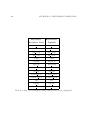
Name
Operator
Definition
Natural join
R icomp S
{(w, z) | Rw ∩ Sz 6= ∅ }
Empty intersection join
R sep S
{(w, z) | Rw ∩ Sz = ∅ }
Superset join
R sup S
{(w, z) | Rw ⊇ Sz }
Proper Superset join
R gtjoin S
{(w, z) | Rw ⊃ Sz }
Equal join
R eqjoin S
{(w, z) | Rw = Sz }
Subset join
R lejoin S
{(w, z) | Rw ⊆ Sz }
Proper subset join
R ltjoin S
{(w, z) | Rw ⊂ Sz }
Non-proper superset join
R !gtjoin S
{(w, z) | Rw 6⊃ Sz }
Non-equal join
R !eqjoin S
{(w, z) | Rw 6= Sz }
Non-subset join
R !lejoin S
{(w, z) | Rw 6⊆ Sz }
Non-proper subset join
R !ltjoin S
{(w, z) |Rw 6⊂ Sz }
Non-superset join
R !gejoin S
{(w, z) | Rw 6⊇ Sz }
Table 2.3: σ-join operators
26
CHAPTER 2. OVERVIEW OF JRELIX
>domain x, y, code intg;
>domain label, colour strg;
>relation Text(x, y, label, colour) <-{(1000, 2000, "text1", "blue"),
(1000, 4000, "text2", "red")};
>relation ColourCode (code, colour) <- {(1, "blue" ), (2, "green"),
(3, "cyan"), (4, "red")};
>pr Text;
+-------------+-------------+----------------------+---------------+
| x
| y
| label
| colour
|
+-------------+-------------+----------------------+---------------+
| 1000
| 2000
| text1
| blue
|
| 1000
| 4000
| text2
| red
|
+-------------+-------------+----------------------+---------------+
relation Text has 2 tuples
>pr ColourCode;
+-------------+----------------------+
| code
| colour
|
+-------------+----------------------+
| 1
| blue
|
| 2
| green
|
| 3
| cyan
|
| 4
| red
|
+-------------+----------------------+
relation ColourCode has 4 tuples
>pr Text icomp ColourCode;
+-------------+-------------+----------------------+-------------+
| x
| y
| label
| code
|
+-------------+-------------+----------------------+-------------+
| 1000
| 2000
| text1
| 1
|
| 1000
| 4000
| text2
| 4
|
+-------------+-------------+----------------------+-------------+
expression has 2 tuples
Figure 2.13: Example of a σ-join operation
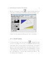
Chapter 3
Overview of Xfig
In this chapter, we give a brief introduction to the Xfig system and the Xfig file format.
We will only focus on the parts of Xfig that are related to the implementation of the
display2D operation.
3.1
Introduction
Xfig is an open source vector graphics editor. It runs on the X Window System on
most UNIX compatible platforms. In Xfig, figures can be drawn using basic objects
such as circles, arcs, polygons, lines, spline curves, text, etc. Images in formats such
as GIF, JPEG, and EPSF (PostScript), can be imported into the graph. The objects
can be created, deleted, moved or modified. Attributes such as colours or line styles
can be selected in various ways. Xfig saves figures in its native text-only Fig format,
but they may be converted into various formats such as PostScript, GIF, JPEG, etc
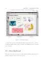
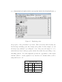
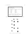
[SS02]. A screen shot of the current Xfig system (Version 3.2.4) [SS02] is shown in
Figure 3.1.
To start Xfig, we use the command “xfig”. To open an existing Xfig file, we use
the following command:
xfig [options] [filename]
The command line options are used to specify the settings of the Xfig window, such
27
28
CHAPTER 3. OVERVIEW OF XFIG
Figure 3.1: Xfig display window
as, window size, the font of the menu, the display background colour, etc. Refer to
the Xfig user manual at http://xfig.org/userman/options.html#options for a detailed
list of options.
3.2
Native Fig Format
The native Fig format is stored in a text file, where the filename ends with “.fig”.
The file contains two parts, a header and objects.
3.2. NATIVE FIG FORMAT
3.2.1
29
Header
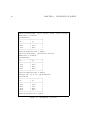
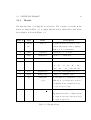
The first nine lines of an Xfig file are its header. The contents of each line in the
header are listed in Table 3.1. A sample Xfig file header, which will be used in the
later chapters, is shown in Figure 3.2
Line #
Type
Name
1
comment
#Fig 3.2
line
Description
contains the name and version of the
current Xfig system. A line beginning
with a ‘#’ is a comment line.
2
string
orientation
“Landscape” or “ Portrait”
3
string
justification
“Center” or “ Flush Left”
4
string
units
5
string
papersize
“Metric” or “ Inches”
“Letter” , “ Legal” , “Ledger” , “Tabloid” ,
“A” , “B” , “ C” , “D” , “E” , “ A4” ,
“A3” , “A2” , “ A1” , “A0” and “B5”
6
float
magnification
export and print magnification, in %
7
string
multiple-page
“Single” or “ Multiple” pages
8
int
transparent
colour
Colour number for transparent colour for
GIF export: -3=background, -2=None,
-1=Default, 0-31 for standard colours
or 32+ for user colours
9
int
resolution coord system
resolution is always 1200 ppi.
Fig units/inches and coordinate system:
1: origin at lower left corner (not used)
2: origin at upper left
Table 3.1: Xfig file header
30
CHAPTER 3. OVERVIEW OF XFIG
#FIG 3.2
Landscape
Center
Metric
Letter
100.00
Single
-2
1200 2
Figure 3.2: A sample Xfig file header
3.2.2
Objects
As defined in the official Xfig documentation [SS02], an Xfig object can be one of
the following seven types.
Type 0 Colour pseudo-object.
Type 1 Ellipse which is a generalization of circle.
Type 2 Polyline which includes polygon and box.
Type 3 Spline (including closed/open approximated/interpolated/xspline spline).
Type 4 Text.
Type 5 Arc.
Type 6 Compound object which is composed of one or more objects.
Type 2, 4 and 6 Xfig objects are relevant to our implementation of the display2D
operation, therefore, we will introduce only these three types.
Type 2 Xfig Object
Type 2 Xfig objects include points, lines, boxes and polylines (open/closed). To
describe a type 2 Xfig object, according to the official Xfig documentation [SS02], we
need two lines of Xfig code. The first line contains the values of all the parameters
from Table 3.2, in order, with each value separated by a blank character. The second
line, beginning with a tab character (‘\t’), gives the coordinates of each point in the
graph, in the order that they are drawn. For example, to display a solid red line, with
a thickness of 2 screen pixels, and with start point (4000, 1500) and end point (3000,
3500), the Xfig code for this line should have the format shown in Figure 3.3.
3.2. NATIVE FIG FORMAT
Type
Parameter
31
Description
Name
Default
Value
int
object code
always 2
2
int
sub type
1: polyline
1
int
line style
enumeration type, line style
0
int
thickness
unit: 1/80 inch or 1 screen pixel
1
int
pen colour
enumeration type, pen colour
0
int
fill colour
enumeration type, fill colour
7
int
depth
enumeration type, layer depth
50
int
pen style
always -1: not used
-1
int
area fill
enumeration type,
-1
fill colour/pattern, -1 = no fill
float
style val
distance between the dots for
0.000
dash line, unit: 1/80 inch.
If solid line, style val = 0.000
int
join style
enumeration type, 0 = Miter join
0
int
cap style
enumeration type, 0 = Butt cap style
0
int
radius
unit: 1/80 inch, radius of arc-boxes
-1
-1 = not used
int
forward arrow
0: off, 1: on
0
int
backward arrow
0: off, 1: on
0
int
npoints
number of points
N/A
Table 3.2: Type 2 Xfig Object Format
2 1 0 2 4 7 50 -1 -1 0.000 0 0 -1 0 0 2
4000 1500 3000 3500
Figure 3.3: Sample Xfig code for a line
32
CHAPTER 3. OVERVIEW OF XFIG
The first number in Figure 3.3 is 2, which is object code that is always 2 for type
2 Xfig objects. It is listed in the first row of Table 3.2. The third number in Figure
3.3 is 0, which corresponds to line style. A value 0 for line style indicates a solid
line. The fourth number, 2, gives the thickness of the line. The fifth number, 4, is
pen colour. A value of 4 for pen colour indicates red. Next we have fill colour which
is 7. A value of 7 for fill colour indicates white. Using the same idea, we can match
the remaining parameters in Table 3.2 to the remaining numbers in the first line in
Figure 3.3. For additional parameter values, refer to Appendix A, Table A.1.
Type 4 Xfig Object
Type 4 Xfig objects are used for text. Only one line of Xfig code is used. Table 3.3
lists the parameters for type 4 Xfig objects. For example, we want to display a text
string “display2D operation” in blue, at coordinates (1975, 2000), at the layer with
depth 49. The Xfig code for this text string is shown in Figure 3.4.
4 0 1 49 -1 0 12 0.000 4 180 1515 1975 2000 display2D operation\001
Figure 3.4: Sample Xfig code for a text string
The first number in Figure 3.4 is 4, which is object code. The third number is 1,
which is text colour. A value of 1 indicates the colour blue . The next number, 49,
gives the depth of the text. The sixth number, 0, gives the font of the text, which
is the default font, Times-Roman. The seventh number, 12, is font size. The eighth
number, 0.000, is angle. Using the same idea, we can match the remaining parameters
in Table 3.3 to the remaining values in Figure 3.4. For additional parameter values,
refer to Appendix A, Table A.1.
Type 6 Xfig Object
Type 6 Xfig objects are used to glue several objects together into one compound
object unit, in a virtual box. The format for the type 6 Xfig object is shown in Table
3.2. NATIVE FIG FORMAT
Type
Parameter
33
Description
Name
Default
Value
int
object
always 4
4
int
sub type
0: Left justified
0
int
text colour
enumeration type, text colour
0
int
depth
enumeration type, layer depth
50
int
pen style
always -1: not used
-1
int
font
enumeration type
0
float
font size
font size in points
12
float
angle
radians, the angle of the text
0.000
int
font flags
bit vector
4
float
height
in fig units, text height
N/A
float
length
in fig units, text length
N/A
int
x, y
coordinate of the origin in fig units
N/A
(the lower left corner of the string)
char
string[ ]
ASCII characters; starts after a blank
N/A
character and ends before the sequence
‘\001’, which is not part of the string.
Table 3.3: Type 4 Xfig Object Format
3.4. The Xfig code for a compound object, that is a combination of the line in Figure
3.3 and the text string in Figure 3.4, is shown in Figure 3.5.
The first number in Figure 3.5 is 6, which is object code. The next four numbers
1935, 1485, 4050 and 3555 give the coordinates of the upper left corner (1935, 1485)
and the lower right corner (4050, 3555) of the box, in which the line and the text
string reside. These box coordinates are calculated by Xfig. The next two lines
represent the line, and are the same as the code appearing in Figure 3.3. The fifth
line is the text string from Figure 3.4. The last number, on its own separate line, is
-6, indicating the end of the compound object.
34
CHAPTER 3. OVERVIEW OF XFIG
Line Number
1
Type
Parameter Name
Description
int
object code
always 6
int
upperleft corner x
Fig units
int
upperleft corner y
Fig units
int
lowerright corner x
Fig units
int
lowerright corner y
Fig units
2 - the 2nd last line
objects
last line
-6
Table 3.4: Type 6 Xfig Object Format
6 1935 1485 4050 3555
2 1 0 2 4 7 50 -1 -1 0.000 0 0 -1 0 0 2
4000 1500 3000 3500
4 0 1 49 -1 0 12 0.0000 4 180 1515 1975 2000 display2D operation\001
-6
Figure 3.5: Sample Xfig code for a compound object
#FIG 3.2
Landscape
Center
Metric
Letter
100.00
Single
-2
1200 2
6 1935 1485 4050 3555
2 1 0 2 4 7 50 -1 -1 0.000 0 0 -1 0 0 2
4000 1500 3000 3500
4 0 1 49 -1 0 12 0.0000 4 180 1515 1975 2000 display2D operation\001
-6
Figure 3.6: A complete Xfig file (including the header from Figure 3.2 and the
object part from Figure 3.5)
Chapter 4
User’s Manual on display2D
In this chapter, we give a tutorial about how to use the display2D operator to
draw a relation. Section 4.1 describes the system requirements for running the
two-dimensional display editor. Sections 4.2 and 4.3 give several detailed examples
showing how to declare a flat relation or a nested relation containing graphical information for displaying text, point, line, triangle, polyline or a combination of these
objects. Section 4.4 explains the syntax of display2D and how to declare a relation
containing vocabulary information. Section 4.5 presents the rules for valid updating
and a series of examples on updating the display.
4.1
Getting Started
The two-dimensional display editor is invoked in jRelix through the display2D operator. The display2D operation displays a relation representing two-dimensional graphs
in a software application called Xfig, which runs on the X Window platform. Therefore before calling the two-dimensional display editor, we must successfully install
Xfig and start the jRelix system. This manual will not elaborate on the installation
process for Xfig, however this information can be found amongst the official Xfig documentation at http://xfig.org/userman/frm installation.html. To start jRelix, go to
the directory where jRelix is installed and type “java JRelix”.
35
36
CHAPTER 4. USER’S MANUAL ON DISPLAY2D
[mimi] [~/JRelix] java JRelix
Starting stand alone JRelix.
+-------------------------------------------+
|
Relix Java version 0.93
|
| Copyright (c) 1997 -- 2005 Aldat Lab
|
|
School of Computer Science
|
|
McGill University
|
+-------------------------------------------+
>
Figure 4.1: Starting jRelix
4.2
Examples of Displaying 2D Graphs Using Flat
Relations
4.2.1
Displaying Text
To display text, a text string and the coordinates of its first letter must be provided.
The text will be shown in a white box with a black border. For example, we want
to print three strings “(5000, 4000)”, “(2000, 4000)” and “(5000, 3000)” at the same
coordinates that appear in each string respectively. We have to declare a relation
containing the strings and then call display2D operator to display the text.
Text
x
y
textstring
5000
4000 (5000, 4000)
2000
4000 (2000, 4000)
5000
3000 (5000, 3000)
Table 4.1: Relation Text
4.2. EXAMPLES OF DISPLAYING 2D GRAPHS USING FLAT RELATIONS 37
domain x intg;
domain y intg;
domain textstring strg;
relation Text(x, y, textstring) <-{
(5000, 4000, "(5000, 4000)"),
(2000, 4000, "(2000, 4000)"),
(5000, 3000, "(5000, 3000)")};
NewText <- display2D ( ) Text;
Figure 4.2: jRelix input for displaying text
After the system has processed the statements from Figure 4.2 as input, an Xfig
window displaying the text strings appears as shown in Figure 4.3. If the user closes
the Xfig window without changing the picture, Text will be assigned to NewText.
Note that a user can customize display properties by defining attributes in a relation, such as: text colour, text font, text font size, line colour, filling colour, etc.
Default values are used where custom properties are not declared. The default colour
is black, the default font is Times-Roman and the default font size is 12.0.
Figure 4.3: Displaying text
38
CHAPTER 4. USER’S MANUAL ON DISPLAY2D
4.2.2
Displaying a Set of Points
To display a set of points, the coordinates of each point must be provided. For
example, if we want to draw three points with coordinates (5000, 4000), (2000, 4000)
and (5000, 3000), the relation containing them is shown in Table 4.2.
Points
x
y
5000
4000
2000
4000
5000
3000
Table 4.2: Relation Points
domain x intg;
domain y intg;
relation Points (x, y) <-{
(5000, 4000),
(2000, 4000),
(5000, 3000)};
NewPoints <- display2D ( ) Points;
Figure 4.4: jRelix input for displaying points
After the system has processed the input from Figure 4.4, an Xfig window displaying three black points appears as shown in Figure 4.5.
4.2.3
Displaying a Set of Labelled Points
To draw the three points from the last example, and with labels containing their
coordinates, we need to add a string type attribute to the relation, which stores
the content for each label. We realize that, after doing this, we end up with a
relation having the exact same form as the relation Text from Table 4.1. In order to
distinguish between these two cases, we require that at least one attribute describing
4.2. EXAMPLES OF DISPLAYING 2D GRAPHS USING FLAT RELATIONS 39
Figure 4.5: Displaying points
the property of the point must be provided. This is necessary when drawing any
labelled shape including point, line, triangle and polyline. In this example, we add
the integer type attribute lc providing the colour of the point, and assign lc to be 0,
which indicates black. Other properties include line width, line style, filling colour,
and filling pattern. Note that display2D provides the opportunity to link certain
attribute names to certain graphical roles, but there are defaults which you’ll be
using until section 4.4.
LabelledPoints
x
y
lc
label
5000
4000
0
(5000, 4000)
2000
4000
0
(2000, 4000)
5000
3000
0
(5000, 3000)
Table 4.3: Relation LabelledPoints
40
CHAPTER 4. USER’S MANUAL ON DISPLAY2D
domain label strg;
domain lc intg;
relation LabelledPoints (x, y, lc, label) <-{
(5000, 4000, 0, "(5000,4000)"),
(2000, 4000, 0, "(2000, 4000)"),
(5000, 3000, 0, "(5000, 3000)")};
NewLabelledPoints <- display2D( ) LabelledPoints;
Figure 4.6: jRelix input for displaying labelled points
Figure 4.7: Displaying labelled points
4.2. EXAMPLES OF DISPLAYING 2D GRAPHS USING FLAT RELATIONS 41
4.2.4
Displaying a Set of Lines
To display a set of lines, the coordinates of the start point and the end point must
be provided.
Lines
x1
y1
x2
y2
1363
3013
2942 3010
2942
3010
3426 1508
3426
1508
2148
583
2148
583
873
1514
873
1514
1363 3013
Table 4.4: Relation Lines
domain x1 intg;
domain y1 intg;
domain x2 intg;
domain y2 intg;
relation Lines(x1, y1, x2, y2) <- {
(1363, 3013, 2942, 3010),
(2942, 3010, 3426, 1508),
(3426, 1508, 2148, 583),
(2148, 583, 873, 1514),
(873,1514, 1363, 3013)};
NewLines <- display2D ( ) Lines;
Figure 4.8: jRelix input for displaying a set of lines
42
CHAPTER 4. USER’S MANUAL ON DISPLAY2D
Figure 4.9: Displaying a set of lines
4.2.5
Displaying a Set of Labelled Lines
Say, we want to draw the lines from the last example, and label each line with a
name. Similar to the example of labelling points, we add a string type attribute label
and an integer type attribute lc.
LabelledLines
x1
y1
1363
3013
2942
x2
y2
lc
label
2942 3010
0
line1
3010
3426 1508
0
line2
3426
1508
2148
583
0
line3
2148
583
873
1514
0
line4
873
1514
1363 3013
0
line5
Table 4.5: Relation LabelledLines
4.2. EXAMPLES OF DISPLAYING 2D GRAPHS USING FLAT RELATIONS 43
relation LabelledLines(x1, y1, x2, y2, lc, label) <-{
(1363, 3013, 2942, 3010, 0,"line1"),
(2942, 3010, 3426, 1508, 0, "line2"),
(3426, 1508, 2148, 583, 0, "line3"),
(2148, 583, 873, 1514, 0, "line4"),
(873,1514,1363,3013, 0, "line5")};
NewLabelledLines <- display2D ( ) LabelledLines;
Figure 4.10: jRelix input for displaying a set of labelled lines
Figure 4.11: Displaying a set of labelled lines
44
4.2.6
CHAPTER 4. USER’S MANUAL ON DISPLAY2D
Displaying a Set of Triangles
To display a set of triangles, the coordinates of the three points of each triangle must
be provided. For example, say we want to draw two triangles. The first triangle
is drawn with a blue border, a yellow filling colour and vertical lines as the filling
pattern. The other triangle is drawn with a yellow border, a blue filling colour and
vertical lines as the filling pattern. Other than the attributes x1, y1, x2, y2, x3, y3
which give the coordinates of the three vertices, we must create three more integer
type attributes: lc, fc and fp. lc stores the border colour. fc stores the filling colour
and fp stores the filling pattern. Note that in Xfig, colours are represented by integers.
A value of 1 indicates blue whereas a value of 6 indicates yellow. The filling pattern
is also associated with integer values. In this case, a value of 50 indicates vertical
lines. Refer to Appendix A, Table A.1 for more information.
Triangle
x1
y1
x2
y2
x3
y3
lc
fc
fp
5000
4000 2000
4000
5000
3000
1
6
50
3000
1000 5000
1000
5000
2500
6
1
50
Table 4.6: Relation Triangle
domain x1, y1, x2, y2, x3, y3, lc, fc, fp intg;
relation Triangle(x1, y1, x2, y2, x3, y3, lc, fc, fp)<-{
(5000, 4000, 2000, 4000, 5000, 3000, 1, 6, 50),
(3000, 1000, 5000, 1000, 5000, 2500, 6, 1, 50)};
NewTriangle <- display2D ( ) Triangle;
Figure 4.12: jRelix input for displaying a set of triangles
4.2. EXAMPLES OF DISPLAYING 2D GRAPHS USING FLAT RELATIONS 45
Figure 4.13: Displaying a set of triangles
4.2.7
Displaying a Set of Labelled Triangles
To draw the triangles from the last example with labels in their centroids, we only need
to add a string type attribute label, since lc, fc and fp are the attributes describing
the properties of a triangle.
LabelledTriangle
x1
y1
x2
y2
x3
5000
4000
2000
4000 5000
3000
1000
5000
1000 5000
y3
lc fc
fp
label
3000
1
6
50
Tri1
2500
6
1
50
Tri2
Table 4.7: Relation LabelledTriangle
46
CHAPTER 4. USER’S MANUAL ON DISPLAY2D
relation LabelledTriangle(x1, y1, x2, y2, x3, y3, lc, fc, fp, label)<- {
(5000, 4000, 2000, 4000, 5000, 3000, 1, 6, 50, "Tri1"),
(3000, 1000, 5000, 1000, 5000, 2500, 6, 1, 50, "Tri2")};
NewLabelledTriangle <- display2D ( ) LabelledTriangle;
Figure 4.14: jRelix input for displaying a set of labelled triangles
Figure 4.15: Displaying a set of labelled triangles
4.2. EXAMPLES OF DISPLAYING 2D GRAPHS USING FLAT RELATIONS 47
4.2.8
Displaying a Sequenced Polyline
To display a sequenced polyline, the coordinates and sequence number of each vertex
must be provided. In section 4.2.4, we had drawn a pentagon from five lines. Now
we will use a relation called Polyline to get the same result.
Polyline
x
y
sq
1363 3013
1
2942 3010
2
3426 1508
3
2148
583
4
873
1514
5
1363 3013
6
Table 4.8: Relation Polyline
Note that in the relation Polyline, the x and y values of the last tuple are the
same as those in the first tuple. (This is a requirement enforced by data structures
in Xfig). It guarantees that the polyline is a closed shape.
If each vertex has a different pen colour or a different filling colour, the first colour
seen will be used and a warning message will be printed in the console.
relation Polyline(x, y, sq) <-{
(1363, 3013, 1),
(2942, 3010, 2),
(3426, 1508, 3),
(2148, 583, 4),
(873, 1514, 5),
(1363, 3013, 6)};
NewPolyline <- display2D ( ) Polyline;
Figure 4.16: jRelix input for displaying a sequenced polyline
48
CHAPTER 4. USER’S MANUAL ON DISPLAY2D
Figure 4.17: Displaying a sequenced polyline
4.2.9
Displaying a Sequenced Polyline with Labelled Vertices
To add a label to each vertex of a polyline, we use the same method as that of labelling
a point, line or triangle. We simply add a string type attribute label and an integer
type attribute lc.
LabelledVertexPolyline
x
y
sq
lc
label
1363
3013
1
0
(1363, 3013)
2942
3010
2
0
(2942, 3010)
3426
1508
3
0
(3426, 1508)
2148
583
4
0
(2148, 583)
873
1514
5
0
(873, 1514)
1363
3013
6
0
(1363, 3013)
Table 4.9: Relation LabelledVertexPolyline
4.2. EXAMPLES OF DISPLAYING 2D GRAPHS USING FLAT RELATIONS 49
relation LabelledVertexPolyline(x, y, sq, lc, label) <-{
(1363, 3013, 1, 0, "(1363, 3013)"),
(2942, 3010, 2, 0, "(2942, 3010)"),
(3426, 1508, 3, 0, "(3426, 1508)"),
(2148, 583, 4, 0, "(2148, 583)"),
(873, 1514, 5, 0, "(873, 1514)"),
(1363, 3013, 6, 0, "(1363, 3013)")};
NewLabelledVertexPolyline <- display2D ( ) LabelledVertexPolyline;
Figure 4.18: jRelix input for displaying a sequenced polyline with labelled vertices
Figure 4.19: Displaying a sequenced polyline with labelled vertices
50
4.3
CHAPTER 4. USER’S MANUAL ON DISPLAY2D
Examples of Displaying 2D Graphs Using Nested
Relations
4.3.1
Displaying a Sequenced Polyline with a Label
If a polyline is closed and it has no self intersection, a label can be displayed in the
centroid of this polyline. To do so, a nested relation is required.
NestedPolyline
label
P1
lc
0
Polyline
x
y
sq
1363
3013
1
2942
3010
2
3426
1508
3
2148
583
4
873
1514
5
1363
3013
6
Table 4.10: Relation NestedPolyline
domain lc intg;
domain Polyline (x, y, sq);
relation NestedPolyline ( label, lc, Polyline)<- {
("P1", 0, {(1363, 3013, 1), (2942, 3010, 2),
(3426, 1508, 3), (2148, 583, 4),
(873, 1514, 5), (1363, 3013, 6)})};
NewNestedPolyline <- display2D ( ) NestedPolyline;
Figure 4.20: jRelix input for displaying a sequenced polyline with a label in its centroid
4.3. EXAMPLES OF DISPLAYING 2D GRAPHS USING NESTED RELATIONS51
Figure 4.21: Displaying a sequenced polyline with a label in its centroid
4.3.2
Displaying Several Polylines or a Combination of Different Shapes
To display several polylines or a combination of different shapes, we have to use a
nested relation. For example, we want to draw the labelled polyline from the previous
section and the labelled triangles from section 4.2.7. We would create a 3-level nested
relation called Graph.
52
CHAPTER 4. USER’S MANUAL ON DISPLAY2D
Graph
NestedPolyline
label
P1
lc
0
LabelledTriangle
Polyline
x
y
sq
1363
3013
1
2942
3010
2
3426
1508
3
2148
583
4
873
1514
5
1363
3013
6
x1
y1
x2
y2
x3
y3
lc
fc
fp
label
5000
4000
2000
4000
5000
3000
1
6
50
Tri1
3000
1000
5000
1000
5000
2500
6
1
50
Tri2
Table 4.11: Nested relation Graph
domain Polyline (x, y, sq);
domain NestedPolyline (label, lc, Polyline);
domain LabelledTriangle (x1, y1, x2, y2, x3, y3, lc, fc, fp, label);
relation Graph (NestedPolyline, LabelledTriangle)<-{
({("P1", 0, {(1363, 3013, 1), (2942, 3010, 2), (3426, 1508, 3),
(2148, 583, 4), (873, 1514, 5), (1363, 3013, 6)})},
{(5000, 4000, 2000, 4000, 5000, 3000, 1, 6, 50, "Tri1"),
(3000, 1000, 5000, 1000, 5000, 2500, 6, 1, 50, "Tri2")})};
NewGraph<-display2D ( ) Graph;
Figure 4.22: jRelix input for displaying a combination of different shapes
4.4. DISPLAYING A GRAPH WITH A VOCABULARY RELATION
53
Figure 4.23: Displaying a combination of different shapes
4.4
Displaying a Graph with a Vocabulary Relation
The formal syntax for the display2D expression is the following:
display2D“(”(V ocabularyExpression)?“)”GraphExpression
|
{z
}
A relational expression
Notice that the VocabularyExpression is optional. In fact, it is a relational expression
which stores the meaning of the attributes in the GraphExpression, which is usually the relational expression that stores the graphical information and needs to be
displayed.
In the previous examples, we left the VocabularyExpression empty. In fact, a
system built-in relation named .vocabulary is used automatically. By printing this
relation shown in Figure 4.24, you will realize that the attributes used in all of the
54
CHAPTER 4. USER’S MANUAL ON DISPLAY2D
previous examples (e.g. x, y, sq, lc, fc, fp, etc) are listed in the relation .vocabulary.
>pr .vocabulary;
+----------------------+----------------------+
| .attribute
| .meaning
|
+----------------------+----------------------+
| x
| cart1
|
| x1
| cart1
|
| x2
| cart1
|
| x3
| cart1
|
| x4
| cart1
|
| y
| cart2
|
| y1
| cart2
|
| y2
| cart2
|
| y3
| cart2
|
| y4
| cart2
|
| sq
| sequence
|
| lc
| line_colour
|
| fc
| fill_colour
|
| tc
| text_colour
|
| fp
| fill_pattern
|
| ls
| line_style
|
| lt
| line_thickness
|
| dl
| dash_length
|
| ft
| font
|
| fs
| font_size
|
| dp
| depth
|
| js
| join_style
|
| cs
| cap_style
|
| fa
| forward_arrow
|
| ba
| backward_arrow
|
+----------------------+----------------------+
relation .vocabulary has 25 tuples
Figure 4.24: Print relation .vocabulary
Note that in the relation .vocabulary, all of the values for the attribute .meaning
are system keywords. For example, “cart1” always means Cartesian coordinate x,
and “cart2” always means Cartesian coordinate y. For more information about the
meaning of other keywords, refer to Appendix A Table A.1.
Now let us look at an example that uses our own defined vocabulary relation. To
display the exact same picture as in section 4.2.1, we begin by defining a relation
Text2, as shown in Table 4.12.
4.4. DISPLAYING A GRAPH WITH A VOCABULARY RELATION
55
Text2
a
b
textstring
5000
4000 (5000, 4000)
2000
4000 (2000, 4000)
5000
3000 (5000, 3000)
Table 4.12: Relation Text2
Comparing this to our example from section 4.2.1, notice that we named the first
two attributes a and b instead of x and y. To let the system know that a actually
means Cartesian coordinate x, and that b actually means Cartesian coordinate y, we
must declare a vocabulary relation which stores such information.
A relation that represents a vocabulary relation must have two attributes. One
attribute is named .attribute with type attribute and the other is named .meaning
with type string. The attribute .meaning is not allowed to have any value other than
those values used by the attribute .meaning in the relation .vocabulary.
TextVocabulary
.attribute
.meaning
a
cart1
b
cart2
Table 4.13: Relation TextVocabulary
Note that the values for the attributes which have meanings “cart1” or “cart2”
can be numeric or string. Now notice that in Table 4.13, we have given meanings to
attributes a and b, but not to attribute textstring. The reason is that any attribute
not shown either in the user defined vocabulary relation or in the relation .vocabulary,
but is shown in the relation that stores graphical information will be treated as a text
string. This text string will be shown in the Xfig window as part of the display.
Finally, to display the relation Texts2, we require both the relations Texts2 and
TextVocabulary.
56
CHAPTER 4. USER’S MANUAL ON DISPLAY2D
Note that in the display2D expression syntax, display2D “(” (Vocabulary-
Expression)? “)” GraphExpression is a relational expression (that has the
same value as GraphExpression only if users do not make changes to the display of
GraphExpression). Because of this, it can be used in assignment (<-), such as in the
input shown in Figure 4.25. In addition to assignment, we can also do all of the
unary operations, including projection, selection and T-selection; or all of the binary
operations, including µ-join and σ-join. For example, in Figure 4.26, we project the
values of attribute textstring from expression display2D (TextVocabulary) Text2.
After the input from Figure 4.26 is processed by the system, an Xfig window appears, showing the same picture as in Figure 4.3. After we close the Xfig window,
the projection result appears on the screen as shown in Figure 4.27.
NewText2 <- display2D (TextVocabulary) Text2;
Figure 4.25: jRelix input for displaying relation Text2 (using Assignment)
pr [textstring] in display2D (TextVocabulary) Text2;
Figure 4.26: jRelix input for displaying relation Text2 (using Projection)
+--------------------+
| textstring
|
+--------------------+
| (5000, 4000)
|
| (2000, 4000)
|
| (5000, 3000)
|
+--------------------+
Figure 4.27: Projection result
4.5
Examples of Updating the Display
Recall that from section 4.2.6, we draw two triangles. We do this first by declaring
a relation named Triangle (shown in Table 4.6). We then input NewTriangle <-
4.5. EXAMPLES OF UPDATING THE DISPLAY
57
display2D ( ) Triangle; into jRelix causing an Xfig window displaying two triangles to appear, as shown in Figure 4.13. Now without doing any modification to
this graph, we close the Xfig window. A new relation NewTriangle as shown in Table
4.14 is created and is assigned to have the same tuples as relation Triangle.
NewTriangle
x1
y1
x2
y2
x3
y3
lc
fc
fp
5000
4000 2000
4000
5000
3000
1
6
50
3000
1000 5000
1000
5000
2500
6
1
50
Table 4.14: Relation NewTriangle
Now we will make updates to the picture. Before we get started, let us understand
some rules for updating.
Rule #1 Updating does not support changing a flat relation to a nested relation. In
another words, introducing a new shape (including point, line, triangle, polyline
and text) into the original graph, or introducing a new polyline into the original
graph which contains a polyline, are not supported by the current system.
Rule #2 Updating must be done without introducing any new attribute into the
relation, when adding, deleting or modifying points, lines, or triangles, or modifying a polyline.
Rule #3 Updating does not support any changes to nested relations or any relations
containing Text.
4.5.1
Valid Updates
1. Flip the top triangle in Figure 4.13 horizontally by using
from the Xfig
toolbar. Then save the figure shown in Figure 4.28.
2. Draw a triangle with a black border, no fill colour and no filling pattern. Then
save the figure shown in Figure 4.29.
58
CHAPTER 4. USER’S MANUAL ON DISPLAY2D
Figure 4.28: After flipping the top triangle
Figure 4.29: After drawing a new triangle
4.5. EXAMPLES OF UPDATING THE DISPLAY
3. Edit the bottom triangle by using
59
to change the filling pattern from
vertical lines to horizontal lines. Then save the figure shown in Figure 4.30.
Figure 4.30: After changing the filling pattern of the bottom triangle
4.5.2
Invalid Updates
4. To increase the width of the border, first click
. Changing the width
from 1 to 4, we get Figure 4.31. Now we go to the Xfig File menu and save the
current figure. An error message window, as shown in Figure 4.32, appears.
The error occurs because the default value for the width is changed from 1 to 4.
Doing this requires a new attribute for the border width/thickness to be added
to the original relation. This violates Rule #2. To fix the problem, we change
the border width back to 1, save the figure, and click “Ok. I fixed it”. The
error message window disappears.
60
CHAPTER 4. USER’S MANUAL ON DISPLAY2D
Figure 4.31: After changing the border width of the bottom triangle
Figure 4.32: Popup error message 1
Figure 4.33: Popup error message 2
4.5. EXAMPLES OF UPDATING THE DISPLAY
61
5. Adding a straight line to the graph, we get Figure 4.34. We are violating
Rule #1, so another error message shown in Figure 4.33 pops up. After fixing
the error and saving the file, we are back again at Figure 4.30. Now we will
exit Xfig. Because of the modification, the relation NewTriangle is no longer
the same as the relation Triangle. Instead the relation NewTriangle, which
represents the new graph shown in Figure 4.30, has a new value showing in
Table 4.15.
Figure 4.34: Adding a line to the graph
NewTriangle
x1
y1
x2
y2
x3
y3
lc
fc
fp
5000
4000 2000
4000
5000
3000
1
6
49
3000
1000 1000
1000
1000
2500
6
1
50
4455
2070 3417
751
2793
2309
0
7
-1
Table 4.15: Relation NewTriangle (after update)
62
CHAPTER 4. USER’S MANUAL ON DISPLAY2D
Here is an example showing a violation of Rule #3. Recall that in section 4.3.2,
we draw two labelled triangles and a labelled polyline from a nested relation named
Graph by calling NewGraph <- display2D ( ) Graph;. Now after adding a rectangular shaped polyline to the graph, and saving the changes, the warning message
shown in Figure 4.36 appears. Note that if the user ignores the error message and
closes the Xfig window, the relation NewGraph will be equal to the unmodified relation Graph.
Figure 4.35: Adding a box to the graph
Figure 4.36: Popup warning message
Chapter 5
Implementation of display2D
In this chapter, we will describe the implementation of the display2D operation.
Section 5.1 gives an overview of the whole implementation, including the overall
architecture of the current jRelix system, the implementation of the display2D syntax,
the display2D syntax tree, the evaluateDisplay2D algorithm and the XfigObj class.
Sections 5.2 and 5.3 describe the detailed implementation of displaying flat and
nested relations. The implementation of updating the display is given in section 5.4.
5.1
5.1.1
Overview
System Architecture
The system used to run display2D contains four parts, the Parser, the Interpreter,
the Execution Engine and the Xfig application. The Parser, the Interpreter and
the Execution Engine are built into the jRelix system. The Xfig application is not
included in jRelix, but is required by the display2D operation to display a relation.
As shown in Figure 5.1, jRelix input from the user is first accepted by the parser,
which parses it and generates a syntax tree. This parser is created by Java Compiler
Compiler (Java CC) [SDV04] , which reads, compiles grammar specifications and
generates a parser. JJTree [SDV04] is a preprocessor for JavaCC. The output of
JJTree is run through JavaCC to create the parser.
63
64
CHAPTER 5. IMPLEMENTATION OF DISPLAY2D
User Input
Parser
Syntax Tree
Interpreter
Xfig
Method Call
Execution Engine
Figure 5.1: System Architecture
The interpreter, implemented as Interprer.java, repeatedly calls the parser, receives
the syntax tree generated by the parser, traverses the syntax tree and decomposes
it into a set of method calls executed by the execution engine. The interpreter also
interacts with the system tables to retrieve and update information about attributes,
relations, views, and computations in the database. For display2D, the interpreter
must generate an Xfig recognizable file and invoke Xfig to display it. If there are any
changes made by the user to the original graph, the interpreter has to analyze the
update and create a new relation presenting the new graph.
In the jRelix system, the execution engine contains the Relation Processor [Hao98],
the Virtual Domain Actualizer [Yua98], the Computation Processor [Bak98], the
Events and Active Database [He97], and the Nested Relation Processor [Hao98].
5.1.2
Building the Display2D Syntax
In section 4.4 we introduced the formal syntax for the display2D expression. The implementation of the display2D syntax is completed with the addition of the following
to the grammar specification file, Parser.jjt.
5.1. OVERVIEW
65
• TOKEN : { < DISP2D : "display2D" > }
We create a token DISP2D using the matched string display2D. The token
DISP2D will be sent to the parser.
• void Display2D () #disp2D : {}
{
<DISP2D> "(" [ Expression() ] ")" Expression()
{ jjtThis.set(OP DISP2D, OP DISP2D); }
}
We define Display2D as a nonterminal. The grammar is <DISP2D> "(" [
Expression() ] ")" Expression() . The root node in the parser tree is
named disp2D.
• void Primary() #void :
{Token t;}
{ Display2D() }
We add the nonterminal Display2D into the specification of Primary(). This
guarantees that <DISP2D> "(" [ Expression() ] ")" Expression() is an
expression.
5.1.3
Examples of the Display2D Syntax Tree
Recall that from section 4.2.1, we draw three text strings by calling NewText <display2D () Text;. The syntax tree for this input is shown in Figure 5.2. In
section 4.4, we draw the same three text strings by calling NewText2 <- display2D
(TextVocabulary) Text2;, where TextVocabulary is a vocabulary relation defined
by the user. The syntax tree is shown in Figure 5.3.
5.1.4
evaluateDisplay2D Algorithm
EvaluateDisplay2D is a function included in the Interpreter.java file. It evaluates the
following relation expression (defined as the display2D syntax in section 4.4):
66
CHAPTER 5. IMPLEMENTATION OF DISPLAY2D
<−
NewText
disp2D
Text
Figure 5.2: Syntax Tree for “NewText <- display2D ( ) Text; ”
<−
NewText2
disp2D
TextVocabulary
Text2
Figure 5.3: Syntax Tree for “NewText2 <- display2D (TextVocabulary) Text2; ”
5.1. OVERVIEW
67
display2D “(” (VocabularyExpression)? “)” GraphExpression
The evaluateDisplay2D function returns a new relation. If the original display is not
updated by the user, the returned relation has the same value as GraphExpression.
Otherwise, the returned relation represents the updated GraphExpression.
To evaluate the display2D expression, the evaluateDisplay2D algorithm first analyzes the syntax tree from display2D. It detects the number of children of node
disp2D. If there is only one child, VocabularyExpression must be empty. Therefore,
only the GraphExpression is loaded. If node disp2D has two children, both VocabularyExpression and GraphExpression are loaded.
After syntax tree analysis, the evaluateDisplay2D algorithm picks an Xfig file
name for the current display. The file name has two parts, the first part is a global
integer which starts at 1, and increases by 1 if the display2D operator is being called
successfully. The other part of the file name is the suffix “.fig”, which indicates an
Xfig file.
In the current directory, the evaluateDisplay2D algorithm creates a file with the
newly picked name, and calls Java I/O facilities to write the Xfig file header, shown
in Figure 3.2, to the current “.fig” file.
The evaluateDisplay2D algorithm is also used to analyze GraphExpression. It
goes through the type of each attribute in GraphExpression. If there is an attribute
with type IDLIST, it indicates that GraphExpression is a nested relation. Then a
global boolean variable nested, with an initial value false, is assigned to be true.
Function dispNestedRel is called to display this nested relation. We will present the
detailed algorithm in section 5.3. If there are no IDLIST type attributes, then
GraphExpression is a flat relation. Function drawRel is called to display this flat
relation. We will explain this in section 5.2.
In addition, the evaluateDisplay2D algorithm uses the Java Runtime.exec() to
invoke Xfig to run the current “.fig” file externally. Also, the algorithm makes a copy
of the current “.fig” file and creates a thread, monitoring whether the user makes any
68
CHAPTER 5. IMPLEMENTATION OF DISPLAY2D
changes to the current display and whether the update is valid. In section 5.4, we
will describe the algorithm for updating the display.
5.1.5
Class XfigObj
Currently, the display2D operation is implemented to display points, lines, triangles,
polylines (open/closed) or text. Therefore, to fulfill the needs of display2D, Xfig
objects with type 2, type 4, and type 6 have been implemented in XfigObj.java.
For display2D, type 2 Xfig objects are used for points, lines, triangles and polylines
(open/closed). In section 4.2.1, we mentioned that any text must appear in a white
box with a black border. This implies that to display text, we need two parts. One
part is a text string and the other is a box with a white filling colour and a black
border colour, which is represented by a type 2 Xfig object. We use type 4 Xfig
objects for the text string, and type 6 Xfig objects to glue the text string and the box
into a compound object.
The file XfigObj.java, which is used to describe an Xfig object, contains the following six parts.
• A group of instances, which are a union of the parameters required by type 2,
4 and 6 Xfig Objects.
• A general constructor XfigObj().
• A constructor XfigObj(int obj type), which can be used to specify the object
type.
• Function findLength(double font size). For a given font size, the function
returns an integer value for the length of a text string in Times-Roman, which
is the default font in Xfig.
• Function outFigFile Objs(). It returns a string containing all the parameters required by type 2 Xfig objects. For display2D, we use this function for
5.2. DISPLAYING 2D GRAPHS USING FLAT RELATIONS
69
points, lines, triangles and polylines. An example of the return value of function
outFigFile Objs() is shown in Figure 3.3.
• Function outFigFile Text(). It returns a string which is the Xfig code for
a compound object containing text strings and a white box with black border. The coordinates of the upper left corner and the lower right corner of the
box are calculated in this function. An example of the return value of function outFigFile Text() is shown in Figure 3.5. Note that in display2D, this
function is only used for text.
5.2
Displaying 2D Graphs Using Flat Relations
In this section, we will use the following example to illustrate how display2D is implemented for displaying a flat relation.
Example: A dummy flat relation named Picture, which stores graphical information needs to be displayed. A dummy flat relation named Vocab will be the
vocabulary relation used for our display operation. To display the relation Picture, we input NewPicture <- display2D(Vocab) Picture;.
5.2.1
Non-Text
In this section, 5.2.1, we assume that the relation Picture does not contain any text
strings. In the next section, 5.2.2, we will introduce text strings to the relation
Picture and show how to deal with them.
As mentioned in section 5.1.4, the evaluateDisplay2D algorithm analyzes the
attributes of the relation Picture and determines that it is a flat relation. Then
function drawRel, which is included in Interpreter.java file is invoked. Before the
relation Picture is displayed in an Xfig window, we need to do the following:
70
CHAPTER 5. IMPLEMENTATION OF DISPLAY2D
Determine the Type of the Graph Represented by the Relation Picture
In the relation Vocab, we go through the values of the attribute .attribute, tuple
by tuple, trying to find matches to the attribute names of the relation Picture.
It there is a match, we get the value of the attribute .meaning from the current
tuple in the relation Vocab. If the value is “cart1”, c1, which is a corresponding
integer variable with an initial value 0, increases by 1. If it is “cart2”, c2, which
is also a corresponding integer variable with an initial value 0, increases by 1.
If it is “sequence”, polyline flag, a global integer variable with a initial value 0,
is assigned to be 1.
After finishing all of the tuples of the relation Vocab, we then compare the
values of c1 and c2.
• If c1 is not equal to c2, throw an exception.
• If c1 = c2 = 2, then the relation Picture is a set of lines.
• If c1 = c2 = 3, then the relation Picture is a set of triangles.
• If c1 = c2 = 1,
* If polyline flag = 1, then the relation Picture represents a polyline.
* If polyline flag = 0, then the relation Picture represents a set of points.
Determine the Number of Objects
From the last step, if a polyline type is detected, it would guarantee that there
is only one polyline from the relation Picture, since it is a flat relation. If
the relation Picture contains a set of points/lines/triangles, the number of
points/lines/triangles is the number of the tuples from the relation Picture.
With the number of objects determined, we declare an array of XfigObj objects.
Extract Information from the Relation Picture
• Non-polyline
5.2. DISPLAYING 2D GRAPHS USING FLAT RELATIONS
71
For each tuple, say tuple i, in the relation Picture, we do the following:
In the relation Vocab, we go through the values of the attribute .attribute,
tuple by tuple, trying to find matches to attribute names of the relation
Picture. It there is a match, we record the column number, v idx, of the
matched attribute in the relation Picture. Then we retrieve the value,
x, from the cell, which is located at row i, column v idx in the relation
Picture.
To reveal the meaning of the value, x, we obtain the value of the attribute
.meaning from the current tuple in the relation Vocab. If the value is
“line colour”, it indicates that the parameter, pen colour, from Table 3.2
has the value x. Please refer to Table A.2 in Appendix A for more cases.
Each time, after we get a new value x and its meaning (cart1, cart2,
line colour, etc), we assign it to the corresponding instance of the XfigObj
object(s) declared earlier. Note that we must keep track of the number of
appearances of “cart1” and “cart2”, because points, lines or triangles have
different pairs of “cart1” and “cart2”.
Note that the values for the attributes which have meanings “cart1” or
“cart2” can be numeric or string. If the values are numerical, the system
will treat the values as the actual coordinates. If the values are strings, the
system will automatically assign positions 1000, 2000, 3000, etc., according
to the sort order of the strings.
• Polyline
To get the graphical information from a relation which is a polyline, we
first determine the total number of vertices, max seq, which equals the total number of tuples in the relation. Then for each integer, starting from
1 to max seq, we find the corresponding tuple, using the same method, described for non-polyline, to get the values for Cartesian coordinate x and
Cartesian coordinate y. Then we store the value in the XfigObj object declared earlier. As mentioned in section 4.2.8, if each vertex has a different
72
CHAPTER 5. IMPLEMENTATION OF DISPLAY2D
pen colour or a different filling colour, the first colour seen will be used
and a warning message will be printed in the console.
Output the XfigObj Objects
First of all, an XfigObj object calls the function outFigFile Objs(), which is
included in the XfigObj.java file, to get a string containing all the parameters
of the object. Then by using Java I/O, we write the return string to the current “.fig” file. Finally, as mentioned in section 5.1.4, the evaluateDisplay2D
algorithm invokes Xfig to run the current “.fig” file externally.
5.2.2
Text
If an attribute of the relation Picture is not shown as a value of the attribute .attribute
in the relation Vocab, the values of this attribute in the relation Picture will be
treated as text strings when displayed in the Xfig window. For now, we call this type
of attribute “text string attribute”. Note that a text string attribute could have any
type, including integer, float, double, short, long and string.
To detect whether text string attributes exist in the relation Picture, we call function isStringin() to check each attribute of the relation Picture. If the current
attribute is in any tuple of the attribute .attribute in the relation Vocab, a true value
is returned. If the opposite occurs, text count, which is an integer variable with an
initial value 0, increases by 1, and as well, we record the current column index number
in an array texts idx.
While checking each attribute of the relation Picture, we also have to be aware
of whether there are any attributes, in the corresponding tuple in the relation Vocab, that have the meaning “line thickness”, “line style”, “line colour” “fill colour”
or “fill pattern”. If there are any such attributes, draw, an integer variable with a
initial value 0, is assigned to be 1. This step is necessary, because to distinguish a
relation representing text from a relation representing text and a shape (including
points/lines/triangles/polyline), we need at least one attribute describing the prop-
5.2. DISPLAYING 2D GRAPHS USING FLAT RELATIONS
73
erty of the shape. We had mentioned this in section 4.2.3.
We could end up with multiple text strings. For example, the relation Picture
could have the form shown in Figure 5.4, where the attributes x and y are the
coordinates and s1, s2 and s3 represent text strings. However, since s1, s2 and s3
share the coordinates (x, y), an overlap of three text strings in a white box with a
black border will be shown.
To avoid overlaps, we must make use of the parameter, depth, from Table 3.2
to make the text appear at different layers in the display. We require that the first
text string attribute in the relation Picture has the depth value 49, and the nth text
string attribute has the depth value 50 −n, where n is less than or equal to 49. i.e.
s1 has depth 49, s2 has depth 48 and s3 has depth 47. Note that larger depth value
indicates that the object is deeper than (under) objects with smaller depth values.
Also, we should move each text string away from each other, since they completely
overlap. If the first text string has coordinates (X, Y), then we assign the nth text
string with coordinates (X+27×(n-1), Y+27×(n-1)). Therefore, if s1 has coordinates
(x, y), then s2 has coordinates (x+27, y+27), and s3 has coordinates (x+54, y+54).
By using the constant 27, which represents 27 Fig units, a very small distance in
Xfig and display independent (the length is the same regardless of the display screen
dimensions), we get the visual effect in Figure 5.5.
Picture (x, y, s1, s2, s3)
Figure 5.4: Multiple text strings in the relation Picture
s1
s2
s3
Figure 5.5: Displaying multiple text
In the flat relation Picture, the number of text strings, is equal to the number
of tuples of the relation Picture times text count. We create an array of XfigObj
objects, text, to store these text strings. We examine each tuple of the relation
74
CHAPTER 5. IMPLEMENTATION OF DISPLAY2D
Picture, by using the same method described for non-text, to get the content of the
text strings, and the values for “text colour”, “font” and “font size”. Then we store
the value in the XfigObj object array text. A text string must have coordinates for
display. According to the type of the graph represented by the relation Picture, the
coordinates for the text string are calculated differently.
Text and Point: Picture (x, y, colour, s1)
In the relation Picture, the attributes x and y are the coordinates. The attribute
colour is the “line colour” and s1 is a text string attribute.
Recall that in Table 3.3, the coordinate location (x, y) for text is the lower
left corner of the text string. Therefore there is an overlap between the point
and the text string. To avoid this, we require that, if the point has coordinates
(X, Y), the corresponding text string must have coordinates (X+180, Y+180),
where the constant 180 represents 180 Fig units and is display independent.
Text and Line: Picture (x1, y1, x2, y2, colour, s1)
In this case, the text string will have the same direction as the slope of the
corresponding line. Also, the text string will be centered at the center of the
line. To do this, we need to find the slope and the coordinates of the middle
point of the corresponding line, and also the length of each text string. Then
we calculate the coordinates for the text string.
Text and Triangle: Picture (x1, y1, x2, y2, x3, y3, colour, s1)
To display a text string with a triangle, we require that the coordinates of the
beginning of a text string are the coordinates of the centroid of the corresponding triangle.
Text and Polyline: Picture (x, y, sq, colour, s1)
Since the relation Picture is a flat relation, we are only able to display text
strings next to each vertex of a polyline. By using the method for locating text
5.3. DISPLAYING 2D GRAPHS USING NESTED RELATIONS
75
strings next to a point, we require that, if a vertex has coordinates (X, Y), the
corresponding text string have coordinates (X+180, Y+180).
In the next section 5.3, we will deal with a text string displayed in the centroid
of a polyline that is closed and has no self intersection.
5.3
Displaying 2D Graphs Using Nested Relations
In this section, we will use the example from section 4.3.2 to illustrate how display2D
is implemented for displaying a nested relation.
Recall that in section 4.3.2, we displayed two labelled triangles along with a
polyline, labelled in its centroid, from the nested relation Graph, as shown in table
4.11. In Figure 5.6, the contents of the relation Graph and its underlying dot relations
.LabelledTriangle, .NestedPolyline and .Polyline are shown. From this, we see that
we can use a tree structure to represent a nested relation. The top level relation is
the root of the tree. Depending on its level in the nested relation, an underlying dot
relation is an intermediate or leaf node of the tree. The tree structure for the nested
relation Graph is shown in Figure 5.7.
As mentioned in section 5.1.4, the evaluateDisplay2D algorithm analyzes the
attributes of the relation Graph and determines that it is a nested relation. Then the
function dispNestedRel which is included in Interpreter.java file is invoked. Before
explaining the algorithm for the function dispNestedRel, we need to also understand
a function named rel Type, which gets called by dispNestedRel.
function rel Type(Relation r)
The function rel Type is used to determine the hierarchy of a node in its corresponding tree structure. The node, which is actually a relation, is passed
to the function which returns an integer value of 1, 2 or 3. A return value 1
indicates that it is the root of the tree. A return value 2 indicates that it is an
intermediate node of the tree. A return value 3 indicates that it is a leaf node
76
CHAPTER 5. IMPLEMENTATION OF DISPLAY2D
Graph
NestedPolyline
LabelledTriangle
1
3
.LabelledTriangle
.id
x1
y1
3
3000
1000
3
5000
4000
x2
y2
x3
y3
lc fc
fp
label
5000 1000
5000
2500
6
1
50
Tri2
2000 4000
5000
3000
1
6
50
Tri1
.Polyline
.NestedPolyline
.id label
lc Polyline
1
0
P1
2
.id
x
y
sq
2
873
1514
5
2
1363
3013
1
2
1363
3013
6
2
2148
583
4
2
2942
3010
2
2
3426
1508
3
Figure 5.6: Nested relation Graph and its underlying dot relations
Graph
.LabelledTriangle
.NestedPolyline
.Polyline
Figure 5.7: A tree structure representation for the nested relation Graph
5.3. DISPLAYING 2D GRAPHS USING NESTED RELATIONS
77
of the tree. To determine the type of Relation r, the function rel Type uses the
following concepts:
Root:
must have no attributes with name “.id”.
Intermediate node:
must have an attribute with name “.id” and at least one attribute, other
than the attribute named “.id”, with type IDLIST.
Leaf node:
must have an attribute with name “.id” and must have no other attributes
with type IDLIST.
Figure 5.8 gives the detailed algorithm for the function dispNestedRel. There are
three parameters passed to the function. String s, is the name of the nested relation,
r, which stores the graphical information and will be displayed. Relation Vocab is the
relation that stores the vocabulary information. Long id is for the surrogate number,
or the values of the attribute .id in the relation r. Note that since the top level (root
node) relation has no attribute named “.id ” and the minimum surrogate number for
a nested relation is 1, we use a value 0 for the long id field. In our example, after the
relation Graph is detected as a nested relation, dispNestedRel(“Graph”, .vocabulary,
0) is called. (.vocabulary is the system built-in vocabulary relation.)
In the dispNestedRel algorithm, we first determine that the relation Graph is a
root node by using the function rel Type. Then we examine its first attribute NestedPolyline, which has a type IDLIST. Therefore, we recursively call the function dispNestedRel(“.NestedPolyline”, .vocabulary, 1), where 1 is the value of the cell located
at row 1, column 1 in the relation Graph, as shown in the Figure 5.6.
Now we use the dispNestedRel algorithm to analyze the relation .NestedPolyline.
First we find out that relation .NestedPolyline is an intermediate node. For each
tuple, the algorithm then does a comparison of the value of the attribute .id in the
relation .NestedPolyline to the current id. In this case, the current id is 1. If they
78
CHAPTER 5. IMPLEMENTATION OF DISPLAY2D
—————————————————————————————————–
dispNestedRel (String s, Relation Vocab, long id)
Find a relation, r, which has the same name as the value of string s.
reltype = rel Type (r);
If reltype == 1
//r is root
For each attribute i of r
If attribute i has type IDLIST
For each tuple j of r
dispNestedRel (“.”+attribute i ’s name, Vocab, data in cell [i ][j ])
If reltype == 2
//r is an intermediate node
For each tuple j of r
If data in cell [0][j ] equal to id
For each attribute i of r
If attibute i has type IDLIST and attribute i’s name is not “.id”
dispNestedRel (“.”+attribute i ’s name, Vocab, data in cell [i ][j ])
If reltype == 3
//r is a leaf node
drawRel (r, Vocab, id)
—————————————————————————————————–
Figure 5.8: Algorithm for the function dispNestedRel
5.3. DISPLAYING 2D GRAPHS USING NESTED RELATIONS
79
are not equal, it indicates that the current tuple does not belong to the current
nested relation tree. If they are equal, we examine the attributes of the relation
.NestedPolyline, until we find that the attribute Polyline has type IDLIST and is
not named “.id”. Then, we recursively call the function dispNestedRel(“.Polyline”,
.vocabulary, 2), where 2 is the value of the cell located at row 1, column 4 in the
relation .NestedPolyline, as shown in the Figure 5.6.
Now we use the dispNestedRel algorithm to analyze the relation .Polyline. After
we detect that it is a leaf node, we simply call drawRel(.Polyline, .vocabulary, 2) for
drawing a flat relation. Note that even though .Polyline is a flat relation, it is still
part of a nested relation tree and therefore, we require the surrogate to be passed to
the function drawRel. In this case, the surrogate is 2. This guarantees that only the
tuples belonging to the current nested relation tree are selected. If a flat relation is
not part of a nested relation tree (i.e. has no attribute .id ), we will pass -1 instead
of the surrogate to the function drawRel.
Following the same idea illustrated above, the function dispNestedRel will traverse
the remaining branches of the tree, calling the function drawRel when leaf nodes are
detected.
The function drawRel will use the exact same method described in section 5.2 to
display the leaf node relation. However, there are four special cases.
1. Text and Polyline
In section 4.3.1, we had shown an example of a text string displayed in the
centroid of a closed polyline having no self intersection. To find the coordinates
of the centroid of such a polyline, we first calculate the area of the polyline from
Formula 1 shown below. Then we use Formulas 2 and 3 to get the centroid
coordinate x and centroid coordinate y. The coordinates of the beginning of
the text string are (xc , yc ).
Formula 1: Area =
Formula 2: xc =
1
2
Pn
1
6×Area
i=1 (xi yi+1
Pn
i=1 (xi
− xi+1 yi )
+ xi+1 )(xi yi+1 − xi+1 yi )
80
CHAPTER 5. IMPLEMENTATION OF DISPLAY2D
Formula 3: yc =
1
6×Area
Pn
i=1 (yi
+ yi+1 )(xi yi+1 − xi+1 yi )
If the polyline has no self intersection and is open, as shown in Figure 5.9, we
just simply connect vertex V1 and V6 by an imaginary line. Therefore, we can
apply Formula 1 to calculate the area, and get the coordinates of the centroid
from Formula 2 and 3.
V6
V1
V5
V2
V4
V3
Figure 5.9: An open polyline
2. Text and Points
Table 5.1 presents a nested relation, NestedPoints, which contains three black
points and a text string “Three Points”. We need to determine the coordinates
of the text string. In this case, we require that for the text string, the x coordinate is the average of the x coordinates of all the corresponding points, and the
y coordinate is the average of the y coordinate of all the corresponding points.
Therefore, the text string “Three Points” has coordinates (3000, 2000).
NestedPoints
label
Three Points
Points
x
y
lc
1000
1000
0
2000
1500
0
6000
3500
0
Table 5.1: Relation NestedPoints
5.3. DISPLAYING 2D GRAPHS USING NESTED RELATIONS
81
3. Text and Lines
Table 5.2 presents a nested relation, NestedLines, which contains three black
lines and a text string “Three Lines”. We need to determine the coordinates of
the text string. In this case, we require that the coordinates of the text string
are the average of the coordinates of the middle points of all the corresponding
lines. For the relation NestedLines, the middle points for the three lines are
(2000, 2000), (3000, 2000) and (4000, 2000). Therefore, by taking the average,
the text string “Three Lines” has coordinates (3000, 2000).
NestedLines
label
Lines
x1
Three Lines
y1
x2
y2
lc
1000
2000 3000
2000
0
2000
3000 4000
1000
0
3000
1000 5000
3000
0
Table 5.2: Relation NestedLines
4. Text and Triangles
Table 5.3 presents a nested relation, NestedTriangles, which contains a text
string “Three Triangles” and three triangles with a black border colour and a
white filling colour. We need to determine the coordinates of the text string.
In this case, we require that the coordinates of the text string are the average
of the coordinates of the centroids of all the corresponding triangles. For the
relation NestedTriangles, the centroid points for the three triangles are (2000,
3000), (3000, 2000) and (1000, 4000). Therefore, by taking the average, the
text string “Three Triangles” has coordinates (2000, 3000).
82
CHAPTER 5. IMPLEMENTATION OF DISPLAY2D
NestedTriangles
label
Triangles
Three Triangles
x1
y1
1000
2000
2000
1000
x2
y2
x3
y3
lc fc
3000 1000
2000
6000
0
7
3000
4000 1000
3000
2000
0
7
1000
1000 3000
1000
8000
0
7
Table 5.3: Relation NestedTriangles
5.4
Updating the Display
The updating algorithm is implemented in detectFileDiffThread.java file. The class
detectFileDiffThread implements the Java Runnable interface and rewrites the method
run() contained in the Runnable interface.
As mentioned in section 5.1.4, the evaluateDisplay2D algorithm creates a copy of
the current “.fig” file. For example, if the current file is named with “1.fig”, then the
copied file is named “ 1.fig”. In the method run(), by comparing the current and the
copied files, we can detect whether there are any updates made by the user.
In Figure 5.10, we give the algorithm for the function run(). Most of the steps
listed in the function run() are self explanatory, however we will pay special attention
to lines 7, 10 and 19 in the algorithm.
• Line 7: How to check if the updates violate the three updating rules
The three updating rules have been introduced in section 4.5. Now after listing
each rule again, we will explain how to check for violations.
Note that according to Rule #3, the relation for the current graph must be a
flat relation. This implies that the Xfig file must only contain a single shape of
either points, lines, triangles or a polyline. All of these shapes are type 2 Xfig
objects, as mentioned in section 5.1.5.
Rule #1 Updating does not support changing a flat relation to a nested relation.
In another words, introducing a new shape (including point, line, triangle,
5.4. UPDATING THE DISPLAY
—————————————————————————————————–
run ()
{
1
while (Xfig display window is not closed by the user)
2
{
3
Compare the current file “ file.fig” and the copied file “ file.fig” by
4
comparing 2 strings that contain the contents of the 2 files
5
if (2 strings are not equal) // there is an update
6
{
7
if (The update does not violate the 3 updating rules in section 4.5)
8
{
9
Call Java Runtime.exec() to run “ cp file.fig file.fig” externally.
10
Create a new relation from the file “ file.fig” .
11
A temporary empty file is created in the current directory.
12
Java I/O outputs the data of the new relation into the file.
13
}
14
if (Violation is detected)
15
{
16
Java Swing is used to create a pop up error message window.
17
}
18
}
19
sleep (3000) // thread is put to sleep for 3 seconds
}
}
—————————————————————————————————–
Figure 5.10: Algorithm for the function run() in detectFileDiffThread.java
83
84
CHAPTER 5. IMPLEMENTATION OF DISPLAY2D
polyline and text) into the original graph, or introducing a new polyline
into the original graph which contains a polyline, are not supported by the
current system.
Polyline
To determine that the original graph is a polyline, we examine the
value of the global integer variable polyline flag, mentioned in section
5.2. If it is 1, it indicates a polyline. Recall that in section 4.2.8, we
had drawn a pentagon from the relation Polyline. The Xfig code for
the pentagon is shown in Figure 5.11.
To determine whether the user adds more objects (points, lines, triangles and polylines) to the original graph, we skip the first nine lines
of the Xfig header and the two lines of code for the pentagon. If we
find that there are additional lines, it indicates there are other objects.
Therefore, these updates would violate Rule #1.
#FIG 3.2
Landscape
Center
Metric
Letter
100.00
Single
-2
1200 2
2 1 0 1 0 7 50 -1 -1 0.000 0 0 -1 0 0 6
1363 3013 2942 3010 3426 1508 2148 583 873 1514 1363 3013
Figure 5.11: Xfig file for a polyline
Non-polyline
If polyline flag is not equal to 1, the current graph is non-polyline.
First, we need to figure out the shape represented by the Xfig file.
The number of points in an Xfig object indicates the shape of the
object. Table 3.2 shows the number of points, npoints, of a type 2
Xfig object in its last parameter listed. If npoints is 1, it represents a
5.4. UPDATING THE DISPLAY
85
point. If npoints is 2, it represents a line. If npoints is 4, it represents
a triangle. (4 is used instead of 3, because a triangle is a closed shape.
This is a requirement enforced by Xfig.) If npoints is greater than 4,
it represents a polyline. In the Xfig code of a type 2 Xfig object, the
value of the last number in the first line represents npoints.
To determine whether there are new shapes introduced to the original
graph, we skip the first nine lines of the Xfig header. Then in the
updated Xfig file, shown in Figure 5.13, we compare the last number
in each line starting with a character ‘2’ (object type code for type 2
Xfig objects, which is always the first character in the first line of a
type 2 Xfig object code), to the last number in the first line starting
with a character ‘2’ in the original Xfig file, shown in Figure 5.12. If
there is a difference, it indicates there are other objects. Therefore,
these updates would violate Rule #1. In our example, the updated
graph represented by the Xfig code in Figure 5.13, violates Rule #1,
since a new shape with a value of 1 for npoints appears.
#FIG 3.2
Landscape
Center
Metric
Letter
100.00
Single
-2
1200 2
2 1 0 1 0 7 50 -1
2000 3000
2 1 0 1 0 7 50 -1
1000 4000
-1 0.000 0 0 -1 0 0 2
2000 1000
-1 0.000 0 0 -1 0 0 2
5000 3000
Figure 5.12: A sample original Xfig file representing non-polylines
Rule #2 Updating must be done without introducing any new attribute into the
relation, when adding, deleting or modifying points, lines, or triangles, or
modifying a polyline.
86
CHAPTER 5. IMPLEMENTATION OF DISPLAY2D
#FIG 3.2
Landscape
Center
Metric
Letter
100.00
Single
-2
1200 2
2 1 0 1 0 7 50 -1 -1 0.000 0 0 -1 0 0 2
2000 3000 2000 1000
2 1 0 1 0 7 50 -1 -1 0.000 0 0 -1 0 0 1
500 2000
Figure 5.13: A sample updated Xfig file representing non-polylines
To determine the existence of additional attributes that violate Rule #2,
we compare the first 15 numbers in the first line of each Xfig object to the
corresponding default values of a type 2 Xfig object, shown in Table 3.2.
An algorithm for this step is given in Figure 5.14.
Rule #3 Updating does not support any changes to nested relations or any
relations containing Text.
To determine that the original graph is from a nested relation, we examine
the value of the global boolean variable nested, mentioned in section 5.1.4.
If it is true, it indicates a nested relation.
To determine if the original graph contains text objects (i.e. non type 2
Xfig objects), we invoke a function called isPolyline. The function isPolyline reads an Xfig file as input, and returns a boolean value that indicates
whether the Xfig file contains objects other than type 2 Xfig objects. The
algorithm for the function isPolyline is simple. We skip the first nine lines
of the Xfig file header. Then we check the first character in each following
line, if it is not equal to ‘2’ (object type code for type 2 Xfig objects), and
it is not equal to ‘\t’, (a tab character is always the first character in the
second line of a type 2 Xfig object code, as mentioned in section 5.1.5),
the function isPolyline returns false.
5.4. UPDATING THE DISPLAY
—————————————————————————————————–
In the original Xfig file:
If all the Xfig objects have default values for all of the 15 parameters
{
In the updated Xfig file:
If there exists one Xfig object having one parameter with a different
value from its corresponding default value.
Then it is a violation to Rule #2.
}
Else, say we find parameter p does not have its corresponding default value.
{
In the updated Xfig file:
If there exists one Xfig object having one parameter, other than
parameter p, with a different value from its corresponding default value.
Then it is a violation to Rule #2.
}
—————————————————————————————————–
Figure 5.14: An algorithm for detecting violations to Rule #2
87
88
CHAPTER 5. IMPLEMENTATION OF DISPLAY2D
After we detect a nested relation or the function isPolyline returns false,
if the user saves any updates, there is a violation to Rule #3.
• Line 10: How to create a relation from an Xfig file
To create a relation from an Xfig file, we need to do the following 4 steps:
1. Determine the number of objects represented by an Xfig file
In Figure 5.15, we show an Xfig file which represents three points. To
determine that there are indeed three objects in the Xfig file, we skip the
first nine lines which are the Xfig file header. Then we count the number
of blocks. A type 2 Xfig object is represented by one block (two lines).
In this example, we detect the three blocks shown below. It indicates that
there are three objects and the new relation should have three tuples.
Block 1:
2 1 0 1 0 7 50 -1 -1 0.000 0 0 -1 0 0 1
2000 4000
Block 2:
2 1 0 1 4 7 50 -1 -1 0.000 0 0 -1 0 0 1
5000 3000
Block 3:
2 1 0 1 0 7 50 -1 -1 0.000 0 0 -1 0 0 1
5000 4000
2. Determine the type of the shape represented by an Xfig file
As mentioned earlier, in an Xfig file, to determine the type of the shape it
represents, we examine the number of points, npoints, in any Xfig object.
In a block, the value of the last number in the first line represents npoints.
In this example, it is 1, which implies that the relation represents points.
Therefore, the relation should have at least two integer attributes, x and y.
5.4. UPDATING THE DISPLAY
89
If a line is detected, we create four integer type attributes, x1, y1, x2, y2.
If a triangle is detected, we create six integer type attributes, x1, y1, x2,
y2, x3, y3. If a polyline is detected, we create three integer type attributes,
x, y, sq.
#FIG 3.2
Landscape
Center
Metric
Letter
100.00
Single
-2 1200
2 1 0 1 0 7 50 -1 -1 0.000 0 0 -1 0 0 1
2000 4000
2 1 0 1 4 7 50 -1 -1 0.000 0 0 -1 0 0 1
5000 3000
2 1 0 1 0 7 50 -1 -1 0.000 0 0 -1 0 0 1
5000 4000
Figure 5.15: An Xfig file representing three points
3. Determine the attributes of the relation
Besides the attributes for the coordinates, the relation may have other
attributes that are used to describe the properties of a shape. To determine
the existence of such attributes, we compare the first 15 numbers in the
first line of each block to the corresponding default values of a type 2 Xfig
object, shown in Table 3.2. If there is a difference, the relation needs an
additional attribute to store it.
For example, in block 2, the fifth number, 4, is not equal to the corresponding default value, 0. Therefore, we must create an integer type attribute to
store the pen colour, which is the fifth parameter shown in Table 3.2. Using the corresponding display2D system keyword for pen colour, we name
this attribute “lc”.
4. Determine the content of each tuple of the relation
Now that the number of tuples and the attributes of the relation are deter-
90
CHAPTER 5. IMPLEMENTATION OF DISPLAY2D
mined, we can fill in the values of our relation tuples. The second line of
each block gives the coordinates of the npoints in order. We simply retrieve
the numbers in the second line and put them in the coordinate attributes
of the corresponding tuple. Next, we obtain the values for the other attributes which store the properties of a shape, if we find non-default values
in the first line of a block. Then we store them in the corresponding tuple.
A relation representing the three points in our example is shown in Table
5.4.
• Line 19: The purpose of putting the thread to sleep
It is not necessary that the first statement in line 3 of the while loop is executed
right after one while loop cycle is done. The reason is that the user needs a
short period of time to manipulate the graph before he/she saves the updated
graph. Three seconds is picked as the inactive time for the thread, because it
is a short period of time. Also it is not a relatively long period for the thread
to sleep, so we will not miss an execution of the while loop if the user saves the
updates while the thread is sleeping.
x
y
lc
2000 4000
0
5000 3000
4
5000 4000
0
Table 5.4: A relation represented by the Xfig file from Figure 5.15
Chapter 6
Conclusions
This chapter summarizes the work accomplished in this thesis and provides suggestions for future research and development.
6.1
Summary
In this thesis, we presented the design and implementation of a two-dimensional
display editor for relations (display2D).
The implementation of the display2D operation has several achievements:
• A new syntax is introduced into the jRelix system. This syntax allows users
to invoke the display2D operator on a declared relation which needs to be displayed.
• The display2D operation provides the jRelix system users with a graphical presentation of the information stored in either flat or nested relations.
• The display2D operation allows users to visually interact with the displayed
data and will generate a new relation from an updated display.
• The display2D operation becomes flexible from the addition of user defined
vocabulary relations, which allow users to provide alternate names for attributes
so that they better describe the graph they represent.
91
92
CHAPTER 6. CONCLUSIONS
By using Xfig as the display tool, the implementation of a graphical user interface
(GUI) for the display2D operation is not necessary. Therefore, to display a relation,
the work is reduced to analyzing a relation and producing its corresponding Xfig file.
As mentioned in chapter 3, Xfig runs on the X Window System, which is not platform
independent. This may limit the use of the display2D operation on other platforms
such as Microsoft Windows environments.
The implementation of display2D provides a flexible and extendable framework. In
chapter 3, we listed the types of graphical objects in Xfig, which include text, points,
straight lines, splines, polylines, polygons, arcs, ellipses, circles, etc. Display2D captures most of these shapes, and with a few modifications we could implement all of
them. In section 4.5, we introduced the three rules for updating the display. Currently, we have not found solutions for all of the updating cases. Therefore, further
research can be focused on this.
6.2
Future Work
6.2.1
Further Xfig Object Implementation
So far we have covered type 2, 4 and 6 Xfig objects, including points, lines, triangles,
open/closed polylines and text. But we could implement the remaining Xfig object
types, type 1, 3, and 5, with the following suggested formats.
Type 1: Ellipse which is a generalization of circle
A general format for the relation representing ellipses and circles can be the
following:
Ellipses (cx, cy, rx, ry)
The attributes cx, cy, rx and ry are integers. (cx, cy) are the coordinates of
the center of the ellipse. rx and ry are the horizontal and vertical radii. For
circles, rx and ry have the same value. We also need to declare the meaning
6.2. FUTURE WORK
93
of the attributes cx, cy, rx and ry in a vocabulary relation, as shown in Table
6.1. Like the keyword “cart1” mentioned in the earlier chapters, “cart1center”,
“cart2center”, “cart1radius” and “cart2radius” will be the system built-in keywords .
.attribute
.meaning
cx
cart1center
cy
cart2center
rx
cart1radius
ry
cart2radius
Table 6.1: A vocabulary relation for ellipses and circles
Type 3: Spline which includes closed/open approximated/interpolated/xspline spline
A general format for the relation representing one spline can be the following:
Spline(x, y, splsq, spltype)
Similar to the polylines from section 4.2.8, the coordinates and sequence number
of each control point in a spline must be provided. (x, y) are the coordinates
of the control point. splsq is the sequence number for the control points. We
need an additional attribute spltype to specify the type of a spline. A list of the
spline types is given in Table 6.2. We also need to declare the meaning of the
attributes splsq and spltype in a vocabulary relation, as shown in Table 6.3.
“spline sequence” and “spline type” will be the system built-in keywords.
Type 5: Arc
A general format for the relation representing arcs can be the following:
Arcs(x1, y1, x2, y2, x3, y3, arctype)
94
CHAPTER 6. CONCLUSIONS
spline type
value
open approximated spline
0
closed approximated spline
1
open interpolated spline
2
closed interpolated spline
3
open x-spline
4
closed x-spline
5
Table 6.2: Spline types
.attribute
.meaning
splsq
spline sequence
spltype
spline type
Table 6.3: A vocabulary relation for splines
(x1, y1 ) and (x3, y3 ) are the coordinates of the start and end points of the arc
respectively. (x2, y2 ) gives the coordinates of a point, other than the start or
end point, on the arc. We also need an additional attribute arctype to specify
the type of the arc. A value of 1 for arctype indicates open ended arcs. A value
of 2 for arctype indicates pie-wedge (closed) arcs. The following vocabulary
relation shown in Table 6.4 needs to be declared. “arc type” will become a
system built-in keyword.
.attribute
.meaning
arctype
arc type
Table 6.4: A vocabulary relation for arcs
6.2.2
Polar Coordinates
The polar coordinates consist of two parts, the radius, r, and the angle, a, and are
defined in terms of Cartesian coordinates by: x = r cos(a), y = r sin(a).
6.2. FUTURE WORK
95
Currently, our implementation of display2D uses the Cartesian coordinate system
to draw graphs from relations. Compared to the Cartesian coordinate system, the
polar coordinate system uses less complicated equations to represent some curves,
such as circle, arc, cardioid, rose curve, etc. Therefore, we could consider introducing
the polar coordinate system into display2D.
We can use the vocabulary relation in Table 6.5 to name the attributes and their
meaning for the polar coordinate system.
.attribute
.meaning
r
polar1
a
polar2
Table 6.5: A vocabulary relation for the polar coordinate system
Now, a relation representing circles or open ended arcs would be simplified to the
following format: CircleArc (r, a).
6.2.3
Text Length
In section 5.1.5, we mentioned that the current implementation of the display2D
operation can approximately calculate, for any font size, the length of a text string
in Times-Roman, which is the default font in Xfig. However, there are 34 more fonts
available in Xfig. Therefore, we need to develop a mechanism which can find the
accurate length of a text string in any font and font size.
6.2.4
A Simpler Method to Label Points with Their Coordinates
Recall that in section 4.2.3, we drew three points with their coordinates labelled next
to them. The relation has the following format: LabelledPoints (x, y, lc, label ). Here,
(x, y) gives the coordinates of the points. The value of the attribute label contains
coordinates (x, y) as a text string. Though the current relation works properly, it
96
CHAPTER 6. CONCLUSIONS
is inefficient since the value of the attribute label repeats the information already
contained in the coordinate attributes x and y.
To simplify the approach, we would like to consider introducing two keywords
“cart1show” and “cart2show”. “cart1show” would be for showing the Cartesian coordinate x and “cart2show” would be for showing the Cartesian coordinate y. A
vocabulary relation containing them is declared in Table 6.6.
.attribute
.meaning
xs
cart1show
ys
cart2show
Table 6.6: A vocabulary relation for cart1show and cart2show
Therefore, the simplified relation LabelledPoints would appear as follows:
LabelledPoints2 (xs, ys)
Hence, the relation shown in Table 6.7 represents the same graph as the relation
from Table 4.3.
xs
ys
5000
4000
2000
4000
5000
3000
Table 6.7: Relation LabelledPoints2
6.2.5
Extending Display Update
• Updating a graph containing text
Updating relations containing text, which violates the updating Rule #3 in
section 4.5, is not currently supported by display2D. To add this feature, we
could develop a method similar to that of updating type 2 Xfig objects, as
described in section 5.4.
6.2. FUTURE WORK
97
Currently, for type 2 Xfig objects, we analyze an Xfig code block, which represents one object.
Block:
2 1 0 1 0 7 50 -1 -1 0.000 0 0 -1 0 0 1
2000 4000
However, for type 4 Xfig objects that represent text, we will need to analyze
the following Xfig code block which contains one text string:
Block:
4 0 1 49 -1 0 12 0.000 4 180 1515 100 100 string\001
• Introducing new attributes into the relation
Any updating that introduces new attributes into the original relation, which
violates the updating Rule #2 in section 4.5, is not supported by the current
implementation. However, there are two possible solutions for this case.
Solution 1: Use DC= don’t care, a null value in jRelix.
As an example, we use Table 6.8, where the relation Points3 contains three
points. While updating the graph which is represented by the relation Points3,
we change the colour of the point with coordinates (100, 500) from its default
colour black to red. Now we are introducing a new attribute “lc”, which is the
system built-in attribute name for point colour. So our new relation could be
the one as shown in part (a) in Figure 6.1. In this case, since the colour of
the other two points remain in black, DC is equivalent to 0, which is the colour
code for black in Xfig.
98
CHAPTER 6. CONCLUSIONS
Points3
x
y
100
500
200
700
400
300
Table 6.8: Relation Points3
UpdatedPoints3
x
y
lc
100
500
4
200
700
400
300
UpdatedPoints3
x
≡
y
lc
100 500
4
DC
200 700
0
DC
400 300
0
(a)
(b)
Figure 6.1: Relation UpdatedPoints3
Solution 2: Use polymorphic relations.
Polymorphism allows the same definitions to be used with different types of
data, resulting in more general and abstract implementations.
By using the polymorphism concept, the updated relation UpdatedPoints3,
shown in Figure 6.2, consists of two relations, which combine polymorphically into one relation. One is a relation containing the point with updated
colour. The other relation contains the original points with the default colour.
UpdatedPoints3
x
y
lc
100
500
4
x
and
y
200 700
400 300
Figure 6.2: Polymorphic relation UpdatedPoints3
6.3. CONCLUSIONS
99
• Updates changing a flat relation to a nested relation
Any updating that changes a flat relation to a nested relation, which violates
the updating Rule #1 in section 4.5, is not supported by the current implementation. For this case, there are several difficulties.
A nested relation contains a root relation and its underlying dot relations. They
are connected by the surrogate number. To create a nested relation based on
an updated flat relation, we would need to trace the system surrogate number,
and group the similar objects in the graph into dot relations.
Moreover, we would have to be concerned with the name of each newly created
dot relation. Recall that in section 2.1.2, we mentioned that the dot relations
are invisible (i.e not shown in the system relation table). However, we have to
pick up a name which is not being used in the current relation table. In addition
the user has to be notified about the name of all the dot relations. This is a
fairly complicated process.
Because of all these difficulties, further research is needed. All the unsolved
cases are open for discussion.
6.3
Conclusions
The display2D operation in jRelix provides an extensive ability for handling interactive information visualization. The display2D operation also provides flexibility with
additional user defined vocabulary relations, which allow users to provide alternate
names for attributes so that they can better describe the graphs they represent. Users
can invoke display2D to visualize relations which contain basic geometric shapes, such
as points, lines, polylines, triangles and text. Moreover, display2D can be used to visualize many arbitrary relations. An example application of such is the visualization
of the matrix form of a Bill of Material (BOM) problem which follows.
To assemble a chair, we need a front part and a back part. The front part contains
a seat, two legs and two screws. The back part has a rest, two legs and two screws.
100
CHAPTER 6. CONCLUSIONS
The relation Chair, containing the assembly and subassembly information, is shown
in Table 6.9. We also declare a vocabulary relation VocabChair, which describes the
meaning of the attributes of the relation Chair, as shown in Table 6.10. Note that
the attribute Quantity of the relation Chair is not defined in the relation VocabChair.
Therefore, the values of the attribute Quantity will be treated as text strings when
displayed in the Xfig window. Although the attributes Assembly and Subassembly
contain string values, the system will automatically assign numerical coordinates to
each tuple as mentioned in section 5.2.1. The matrix form of the relation Chair is
shown in Figure 6.4.
Chair
Quantity Assembly
Subassembly
1
Front
Seat
2
Front
Leg
2
Front
Screw
1
Back
Rest
2
Back
Leg
2
Back
Screw
Table 6.9: Relation Chair
ChairVocab
.attribute
.meaning
Assembly
cart1
Subassembly
cart2
Table 6.10: Relation ChairVocab
6.3. CONCLUSIONS
101
domain Quantity intg;
domain Assembly strg;
domain Subassembly strg;
relation Chair(Quantity, Assembly, Subassembly)<- {
(1,
"Front",
"Seat"),
(2,
"Front",
"Leg"),
(2,
"Front",
"Screw"),
(1,
"Back",
"Rest"),
(2,
"Back",
"Leg"),
(2,
"Back",
"Screw")};
relation ChairVocab(.attribute, .meaning) <- {
("Assembly", "cart1"), ("Subassembly", "cart2")};
DispChair <- display2D (ChairVocab) Chair;
Figure 6.3: jRelix input for displaying the matrix form of the relation Chair
Back
Front
2
2
Leg
Rest
1
Screw
2
2
Seat
1
Figure 6.4: Matrix form of the relation Chair
Appendix A
Keywords in Display2D
This appendix presents the keywords used in the vocabulary relations for Display2D
and their corresponding meanings and values in Xfig.
Table A.1: Keywords in vocabulary relations for display2D
Keyword for
Meaning
Value
display2D
-1= Default = Black, 0= Black, 1= Blue
line colour
Point/border colour
2= Green, 3= Cyan, 4= Red
5= Magenta, 6= Yellow, 7= White
8-11 = four shades of blue (dark to lighter)
12-14 = three shades of green (dark to lighter)
fill colour
Filling colour
15-17 = three shades of cyan (dark to lighter)
18-20 = three shades of red (dark to lighter)
21-23 = three shades of magenta (dark to lighter)
24-26 = three shades of brown (dark to lighter)
text colour
Text colour
27-30 = four shades of pink (dark to lighter)
31 = Gold
Continued on next page.
102
103
Keyword for
Meaning
Value
display2D
fill pattern
Filling pattern
-1 = not filled, 0 = black
1-19 = ”shades” of the colour, darker to lighter
Shade: defined as the colour mixed with black
20 = full saturation of the colour
21-39 = ”tints” of the colour, the colour to white
A tint is defined as the colour mixed with white
40 = white, 41 = 30 degree left diagonal pattern
42 = 30 degree right diagonal pattern
43 = 30 degree crosshatch
44 = 45 degree left diagonal pattern
45 = 45 degree right diagonal pattern
46 = 45 degree crosshatch
47 = horizontal bricks, 48 = vertical bricks
49 = horizontal lines, 50 = vertical lines
51 = crosshatch
52 = horizontal ”shingles” skewed to the right
53 = horizontal ”shingles” skewed to the left
54 = vertical ”shingles” skewed one way
55 = vertical ”shingles”skewed the other way
56 = fish scales, 57 = small fish scales
58 = circles, 59 = hexagons, 60 = octagons
61 = horizontal ”tire treads”
62 = vertical ”tire treads”
line style
Line style
-1 = Default, 0 = Solid, 1 = Dashed
2 = Dotted, 3 = Dash-dotted
4 = Dash-double-dotted
5 = Dash-triple-dotted
line thickness
Line width
Any int between 0 to 1000, inclusive.
Continued on next page.
104
APPENDIX A. KEYWORDS IN DISPLAY2D
Keyword for
Meaning
Value
display2D
depth
layer depth
Any int between 0 to 999, inclusive.
Larger value means object is deeper than
(under) objects with smaller depth
font
Font
-1 = Default font = 0 = Times Roman
1 = Times Italic, 2 = Times Bold
3 = Times Bold Italic, 4 = AvantGarde Book
5 = AvantGarde Book Oblique
6 = AvantGarde Demi
7 = AvantGarde Demi Oblique
8 = Bookman Light, 9 = Bookman Light Italic
10 = Bookman Demi, 11 = Bookman Demi Italic
12 = Courier, 13 = Courier Oblique
14 = Courier Bold, 15 = Courier Bold Oblique
16 = Helvetica, 17 = Helvetica Oblique
18 = Helvetica Bold, 19 = Helvetica Bold Oblique
20 = Helvetica Narrow
21 = Helvetica Narrow Oblique
22 = Helvetica Narrow Bold
23 = Helvetica Narrow Bold Oblique
24 = New Century Schoolbook Roman
25 = New Century Schoolbook Italic
26 = New Century Schoolbook Bold
27 = New Century Schoolbook Bold Italic
28 = Palatino Roman, 29 = Palatino Italic
30 = Palatino Bold, 31 = Palatino Bold Italic
32 = Symbol, 33 = Zapf Chancery Medium Italic
34 = Zapf Dingbats
Continued on next page.
105
Table A.1 – continued from previous page
Keyword for
Meaning
Value
display2D
font size
Font size
dash length
The distance between
Any int between 1 to 500, inclusive.
unit: in 1/80 inches
the dots for dash line
join style
Join style
0 = Miter, 1 = Round, 2 = Bevel
cap style
Cap style
0 = Butt, 1 = Round, 2 = Projecting
forward arrow
Arrow type
0 = Stick-type, 1 = Closed triangle
backward arrow
Arrow type
2 = Closed with ”indented” butt
3 = Closed with ”pointed” butt
cart1
Cartesian coordinate x
-
cart2
Cartesian coordinate y
-
sequence
Polyline vertex
Any integer >= 1
sequence number
Table A.1: Keywords in vocabulary relations for display2D
106
APPENDIX A. KEYWORDS IN DISPLAY2D
Xfig Object
Keyword for
Parameter Name
disply2D
line style
line style
thickness
line thickness
pen colour
line colour
fill colour
fill colour
depth
depth
area fill
fill pattern
style val
dash length
join style
join style
cap style
cap style
forward arrow
forward arrow
backward arrow
backward arrow
font
font
font size
font size
text colour
text colour
Table A.2: Xfig object parameter names and the keywords for display2D
Bibliography
[Ado06]
Adobe. Adobe Premiere Pro. Computer Software, 2006.
[Ahl96]
Christopher Ahlberg. Spotfire: An information exploration environment.
ACM SIGMOD Record, 25(4):25–29, December 1996.
[AWS92]
Christopher Ahlberg, Christopher Williamson, and Ben Shneiderman. Dynamic queries for information exploration: an implementation and evaluation. In Proceedings of the SIGCHI conference on Human factors in
computing systems, 1992.
[Bak98]
Patrick Baker. Design and implementation of database computations in
Java. Master’s thesis, McGill University, Montreal, Canada, 1998.
[BEW95]
Richard Becker, Stephen Eick, and Allan Wilks. Visualizing network data.
IEEE Transactions on Visualization and Computer Graphics, 1(1):16 – 28,
March 1995.
[Bur86]
P.A. Burrough. Principles of geographical information systems for land
resources assessment. Oxford: Clarendon Press, New York, 1986.
[CC96]
Tiziana Catarci and Isabel F. Cruz. Information visualization. ACM
SIGMOD Record, 25(4):14 – 15, December 1996.
[Cha02]
Andy Chang. Implementation of sigma-joins in a nested relational language. Master’s thesis, McGill University, Montreal, Canada, 2002.
107
108
[Che01]
BIBLIOGRAPHY
Yuling Chen. A GIS editor for a database programming language. Master’s
thesis, McGill University, Montreal, Canada, 2001.
[CMS99]
Stuart K. Card, Jock Mackinlay, and Ben Shneiderman. Information
visualization. Using vision to think. Morgan Kaufmann, San Francisco,
CA, 1999.
[Cod70]
E. F. Codd. A relational model of data for large shared data banks.
Communications of the ACM, 13(6):377–387, June 1970.
[CRY96]
Stuart Card, George Robertson, and William York. The WebBook and
the Web Forager: An information workspace for the world-wide web. In
Proceedings of the SIGCHI conference on Human factors in computing
systems: common ground, 1996.
[ER93]
Max Egenhofer and James Richards. Exploratory access to geographic
data based on the map-overlay metaphor. Journal of Visual Languages
and Computing, 4(2):105–125, 1993.
[ESJ92]
Stephen Eick, Joseph Steffen, and Eric Sumner Jr. Seesoft - a tool for visualizing line oriented software statistics. IEEE Transactions on Software
Engineering, 18(11):957 – 968, November 1992.
[Fur81]
George Furnas. The fisheye view: a new look at structured files. Bell
Laboratories technical memorandum, 1981.
[GEC98]
Nahum Gershon, Stephen G. Eick, and Stuart Card. Information visualization. Interactions, 5(2):9 – 15, March/April 1998.
[Ger75]
R. Gerritsen. The relational and network models of data bases: Bridging
the gap. 2nd USA-Japan Computer Conference, 1975.
[Hao98]
Biao Hao. Implementation of the nested relational algebra in Java. Master’s thesis, McGill University, Montreal, Canada, 1998.
BIBLIOGRAPHY
[He97]
109
Hongbo He. Implementation of nested relations in a database programming language. Master’s thesis, McGill University, Montreal, Canada,
1997.
[Ins81]
Alfred Inselberg. N-dimensional graphics. Part I - Lines and Hyperplanes,
1981. in IBM LASC Tech.
[Ins90]
Alfred Inselberg.
Parallel coordinates: a tool for visualizing multi-
dimensional geometry. In Proceedings of the 1st conference on Visualization ’90, pages 361 – 378, 1990.
[JS91]
Brian Johnson and Ben Shneiderman. Tree-Maps: a space-filling approach
to the visualization of hierarchical information structures. In Proceedings
of the 2nd conference on Visualization ’91, pages 284 – 291, 1991.
[Kan01]
Sung Soo Kang. Implementation of functional mapping in a nested domain
algebra. Master’s thesis, McGill University, Montreal, Canada, 2001.
[KPS97]
Harsha Kumar, Catherine Plaisant, and Ben Shneiderman. Browsing hierarchical data with multi-level dynamic queries and pruning. International
Journal of Human-Computer Studies, 41(1):103–124, 1997.
[Mac86]
Jock Mackinlay. Automating the design of graphical presentations of relational information. ACM Transactions on Graphics (TOG), 5(2):110 –
141, April 1986.
[Mac04]
Macromedia. Macromedia Director. Computer Software, 2004.
[Mac05]
Macromedia. Macromedia Flash. Computer Software, 2005.
[MB95]
Tamara Munzner and Paul Burchard. Visualizing the structure of the
World Wide Web in 3D hyperbolic space. In Proceedings of the first
symposium on Virtual reality modeling language, pages 33–38, 1995.
[Mer84]
T. H. Merrett. Relational Information Systems. Reston Publishing Co.,
1984.
110
[Mer99]
BIBLIOGRAPHY
T. H. Merrett.
Basics: About data. relational information systems.
http://www.cs.mcgill.ca/∼cs612/relationTxt.ps, September 1999.
[Mer01]
T. H. Merrett. Attribute metadata for relational OLAP and data mining.
In Proceedings, Eighth Biennial Workshop on Data Bases and Programming Languages, pages 65–76, Roma, Italy, 2001.
[NSP96]
Chris North, Ben Shneiderman, and Catherine Plaisant. User controlled
overviews of an image library: a case study of the visible human. In
Proceedings of the first ACM international conference on Digital libraries,
pages 74–82, Bethesda, Maryland, United States, 1996.
[PMR+ 96] Catherine Plaisant, Brett Milash, Anne Rose, Seth Widoff, and Ben Shneiderman. Lifelines: visualizing personal histories. In Proceedings of the
SIGCHI conference on Human factors in computing systems: common
ground, 1996.
[RC94]
Ramana Rao and Stuart Card. The Table Lens: merging graphical and
symbolic representations in an interactive focus + context visualization for
tabular information. In Proceedings of the SIGCHI conference on Human
factors in computing systems: celebrating interdependence, pages 318 –
322, 1994.
[RM93]
George Robertson and Jock Mackinlay. The document lens. In Proceedings of the 6th annual ACM symposium on User interface software and
technology, pages 101 – 108, Atlanta, Georgia, United States, 1993.
[RMC91]
George Robertson, Jock Mackinlay, and Stuart Card. Cone Trees: animated 3D visualizations of hierarchical information. In Proceedings of the
SIGCHI conference on Human factors in computing systems: Reaching
through technology, pages 189 – 194, 1991.
BIBLIOGRAPHY
[SDV04]
111
Sriram Sankar, Rob Duncan, and Sreenivasa Viswanadha.
Compiler
Compiler
(JavaCC)
-
the
Java
parser
Java
generator.
https://javacc.dev.java.net/, 2004.
[Shn92]
Ben Shneiderman. Tree visualization with tree-maps: 2-D space-filling
approach. ACM Transactions on Graphics (TOG), 11(1):92 – 99, January
1992.
[Shn96]
Ben Shneiderman. The eyes have it: a task by data type taxonomy for
information visualizations. In Proceedings of the 1996 IEEE Symposium
on Visual Languages, pages 336 – 343. IEEE Computer Society, September
1996.
[SM97]
H. Shiozawa and Y. Matsushita. WWW visualization giving meanings
to interactive manipulations.
In Proceedings of the Seventh Interna-
tional Conference on Human-Computer Interaction (HCI International
’97), 1997.
[SS02]
Brian V. Smith and Tom Sato.
Xfig user manual, version 3.2.4.
http://xfig.org/userman/, December 2002.
[Sun00]
Weizhong Sun. Updates and events in a nested relational programming
language. Master’s thesis, McGill University, Montreal, Canada, 2000.
[Wan02]
Zongyan Wang. Implementation of distributed data processing in a database programming language. Master’s thesis, McGill University, Montreal,
Canada, 2002.
[WS92]
Christopher Williamson and Ben Shneiderman.
The dynamic Home-
Finder: evaluating dynamic queries in a real-estate information exploration system. In Proceedings of the 15th annual international ACM SIGIR conference on Research and development in information retrieval,
pages 338 – 346, 1992.
112
[Yua98]
BIBLIOGRAPHY
Zhongxia Yuan. Implementation of the domain algebra in Java. Master’s
thesis, McGill University, Montreal, Canada, 1998.
[Zhe02]
Yi Zheng. Abstract data types and extended domain operations in a
nested relational algebra. Master’s thesis, McGill University, Montreal,
Canada, 2002.

Top types

Top brands

Top types

Top brands

Top types

Top brands

Top types

Top brands

Top types

Top brands

Top types

Top brands

Top types

Top brands

Top types

Top brands

Top types

Top brands

Top types

Top brands

Top types

Top brands

Top types

Top brands

Top types

Top brands

Download - McGill School Of Computer Science