Download User Manual of LocalDiff Version 1.5

User Manual of LocalDiff
Version 1.5
Nicolas Duforet-Frebourg and Michael G.B. Blum
Université Joseph Fourier,
Centre National de la Recherche Scientifique,
Laboratoire TIMC-IMAG, Grenoble, France.
September 2013
1
1
Introduction
LocalDiff provides Bayesian measures of local genetic differentiation to characterize non-stationary patterns of isolation by distance. Non-stationary
patterns of isolation by distance arise when genetic differentiation between
populations (or between individuals) increases at different rates in different
regions of the species’ range. Typical patterns include barriers to gene flows,
secondary contact zone, corridors for gene flow, or gradients of gene flow
across the species’ range.
Local genetic differentiation for a sampled populations is defined as the
average genetic differentiation between the sampled population and fictive
neighboring populations. To avoid defining populations in advance, LocalDiff
can also be applied at the scale of individuals. Inference of local genetic differentiation relies on a matrix of pairwise similarity or dissimilarity between
populations or individuals such as matrices of correlation or of FST between
pairs of populations. Local differentiation estimates depend on internal parameters of the method (correlogram parameters) [2]. A MCMC algorithm is
used to integrate local differentiation estimates over the unknown parameter
values.
2
2.1
Starters
Download
An archive containing the software can be downloaded at the following webpage:
http://membres-timc.imag.fr/Michael.Blum/LocalDiff.html
2.2
Windows OS
If you are using windows (64 bits), you can directly use the software
LocalDiff.exe . The first one is the command line software. You have
to open a terminal first (run, then type cmd). Then go in the directory
containing the executable file LocalDiff.exe, and just type LocalDiff.exe
with the parameters of your choice.
2.3
UNIX OS
Extraction and Compilation The archive of the program is provided
with a Makefile for UNIX OS. Go to the directory ArchiveLocalDiff and
compile the local modified Lapack library ([1]).
MyMachine $> make lapack
Then, compile the program
2
MyMachine $> make
After compilation, if for some reasons, you want to clean the directory
of all executables and binary files (including Lapack objects), just type
MyMachine $> make realclean
If you want to remove all executables and binary files but Lapack objects,
just type
MyMachine $>make clean
After compilation, you can run the program. You can run it without
parameters, and a presentation screen will be displayed. Then the software
is run as other usual software for LINUX.
2.4
MAC OS
The software has been initially developped for UNIX type of operating system. It should be running fine with MAC OS. However for recent MAC OS
versions, you need to install Xcode from App Store to make the command
line make works.
Then start Xcode, go to Xcode->Preferences->Downloads and install
component named Command Line Tools. After that all the relevant tools
will be placed in the /usr/bin folder and you will be able to use basic
command lines.
3
Command line
Here is a complete list of the parameters of the program, and their meaning.
When a parameter can be unspecified, it is explicitly mentioned. Basically
the command line to run the software is the following one:
MyMachine $> ./LocalDiff -c genetic_Measure MatrixFile datatype
-i INPUTFile -p PositionFile -o OUTPUTFile -f fast
-l LabelFile -n number_of_neighbors distance_to_neighbors
-s number_of_posterior_replicates -m doMean -v verbose
-d distance_type
-i INPUTFile The input file is the name, with the path, of the file containing the pairwise matrix of correlation, or any other relevant pairwise measure
you want to estimate locally. The input file can also contain genotype data
when using the -c option.
3
-c genetic_Measure MatrixFile datatype LocalDiff can also handle
files of genotypes such as structure’s input files and then compute genetic
measures of similarity. The first argument genetic\_Measure specifies the
(dis)similarity measure to compute. It can be equal to Cov, Cor or Fst,
which are shortcuts for covariance, correlation of allele frequencies between
populations, and Fst measures as described by Weir and Cockerham [4].
The second argument MatrixFile gives the name of the file containing the
pairwise matrix. The third argument datatype tells what kind of data are
in the file. It can be either HaploSNP (0 and 1), DiploSNP (0, 1 and 2)
or MultiAllelic for microsatellites or others. WARNING: if you use this
option, the -c option should be the first option to specify, see example 3 of
subsection 8.3 for instance.
-p PositionFile The position file gives the coordinates of all sampled populations or individuals. The positions can either be Cartesian coordinates
or the longitude and the latitude of the sampling sites (longitude should be
the first coordinate).
-o OUTPUTFile The output file is the name, and path, of the output
file, which contains the locations and local differentiation values for sampled
sites.
-f 1 Use a fast version of the software, if your matrix data contains thousands of sampled sites. Results are only slightly different. Integration of
local differentiation is performed by integration over the prior instead of the
posterior.
-l LabelFile The label file may not be specified. It contains the name of
the sampled populations or individuals of the data set. Default labels are
"pop1, pop2... popn".
-n number_of_neighbors distance_to_neighbors Here are specified the parameters that define the neighborhoods. The first parameter is
the number of fictive neighboring populations in the vicinity of each sampled
site. The second parameter is the distance between the sampling site and its
neighbors. The unit for the distance corresponds to the Euclidean distance
when using Cartesian coordinates and is in kilometer when using longitude
and latitude. By default, LocalDiff considers 2 neighbors and uses a distance
between neighbors and sampling sites equal to one tenth of the minimum
distance between sampling sites.
4
-s number_of_posterior_replicates Estimates of local differentiation
are averaged over posterior replicates of the parameters of the correlogram
model. By default, the number of posterior replicates is equal to 100.
-m doMean Set this parameter to 1 to have local differentiation averaged
over unsampled sites and over replicates of the posterior distribution. For
details of those values, set this parameter to 0. Default value is 1.
-v verbose This parameter specifies the level of details to output from the
execution. Possible values are 0, 1 or 2. Default value is 1.
-d distance_type The coordinates in the PositionFile can be Euclidean
coordinates, or geographic coordinates consisting of longitudes and latitudes.
The distance_type argument must be chosen according to the coordinate
system. The value can be euclidean, for standard euclidean coordinates,
or greatcircle if positions are geographic coordinates. Default value is
euclidean.
4
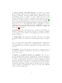
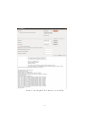
Graphical User Interface
If you are not familiar with command line, you may prefer the GUI program
of the archive. This program is a simple user-friendly interface that runs LocalDiff. All the slots to fulfill correspond to arguments of the command line.
You can see for example figure 4. To run the software correctly, LocalDiff
and the GUI must be in the same directory. To create LocalDiffGUI, you
need to run the script install.sh in the GUI directory.
5
5.1
Files
Input Files
Similarity Matrix Estimates of local differentiation can be computed for
any type of pairwise measures of similarities between populations or individuals, provided that they decrease with geographical distance. Classical
measures include the Pearson correlation, one minus Fst values, identity by
state or by descent measures...
Whatever the choice of statistic, the input file should be the same. Each
line of the input file corresponds to one row of the matrix, and all features
are separated by at least one blank. An example of a 4×4 matrix is provided
below.
5
Figure 1: the Graphical User Interface for LocalDiff
6
1
0.79 0.85 0.82
0.79
1
0.80 0.80
0.85 0.8
1
0.89
0.82 0.9 0.89
1
A matrix of larger dimension, which is used in example 1, is provided in
Examples/Matrix1D.dat.
Genotypes LocalDiff can also compute similarity measures from genotypes, and then use those measures in the algorithm. The file must be a
(nsam × (nbM arkers + 1)) matrix as for the software structure. The first
column corresponds to the population labels, integers from 1 to n. If a LabelFile is used, the labels must be the position of the population label in the
label file e.g an individual with label 1 would be of the first population in the
labelfile, and so on. The order of the individuals does not matter. Missing
values are allowed and must be coded with the value −9.
An example of genotype file is provided below.
3
1
2
1
0 0
1 ...
0 1 −9 ...
1 −9 0 ...
1 1
1 ...
...
A matrix of larger dimension, which is used in example 3, is provided in
Examples/GenoBarrier2D.dat.
Positions All sampled sites (populations or individuals) should be georeferenced. The coordinates can either be Cartesian coordinates or geographic coordinates (longitude followed by latitude). Each line of the file
corresponds to one sampling site with its associates coordinates. If you are
using longitude and latitude, the order matters and longitude must be specified first. Beware, the software checks for number of sites, and number of
individuals/populations in the matrix to be the same. If they are different,
the program stops with the following message:
The Number of populations in the position file does not correspond
to the dimension of the input matrix
An example with 4 sampling sites is provided below
1
1
1
1
1
2
4
7
7
The position file of example is provided in Examples/Position1D.dat.
Labels The label file, is an optional input file. It gives names to individuals/populations of your dataset to be printed in the output files. If no
name is mentioned, default names would be pop1, pop2... To complete the
previous example with 4 sampling sites, an appropriate label file is
M ichael Sean Eric Olivier
5.2
Output File
For the sack of simplicity there is only one output file that is generated after
a run of LocalDiff. Its name is specified with the -o option. If one averages
over replicates and neighbors (-m 1), the file is a n × 4 array. Every line
describes one sampled site. The four columns corresponds to the name of
the population, the two coordinates, and the mean value of local genetic
differentiation.
In the case of a detailed output (-m 0), the output file is an array of
dimensions ((n × nu ) × (nsimu + 4)) where n is the number of sampled population, nu is the number of unsampled neighbors by population, and nsimu
is the number of parameters simulated. Each row corresponds to one unsampled population. The first column is the name of the closest sampled
population. The second column is the index of this neighbor for the sampled
population. Columns three and four are the coordinates of this neighbor.
Then the remaining nsimu columns are the local differentiation values, one
for each value of simulated parameter.
A typical output file with no labels would look like
pop1 1 0.9 1 0.012 ...
pop1 2 1.1 1 0.013 ...
pop2 1 1.9 1 0.014 ...
...
Note: save a logfile To save a journal of the run, redirect the flow in a
log file by typing MyMachine $> ./LocalDiff ... > myLocalDiffRun.log
Note: using -c If you are using the pairwise statistic calculation on genotypic data (FST , correlations, or covariances), you will have a second output
file. This file is the second argument of the -c option and contain the matrix
of pairwise statistics. So you can use LocalDiff as a quick way to compute
statistic on your data.
8
6
6.1
Displaying the results with a Local Genetic Differentiation map
Advocated tools
LocalDiff does not provide any visualization tool for displaying Local Genetic
Differentiation map. Thus the software remains really easy to use on any
computer, without calling graphical libraries. Displaying a Local Genetic
Differentiation map after a run of LocalDiff can be performed with the R
software, and the packages sp and fields.
A possibility is to display a map of LocalDiff values using a grid that
spans the range of the data. This is done by using another layer of Kriging,
in a much more classical way this time. How to display the results with R
is shown afterwards for two different examples.
7
Non-stationarity test
To ascertain the bias in local genetic differentiation measures due to uneven
sampling, we use the following test routine:
Data: sampling scheme
Create a grid of m × n locations with equally distant neighbors dx;
Map the sampling scheme of the data to the grid, by labelling each
closest neighbor in the grid of a location in a data set;
Create a batch of parameters to integrate over parameters such as
migration rates, effective population sizes..;
for all parameters considered do
Simulate a 2-dimensional stepping-stone model with ms on a
regular grid;
Keep only individuals sampled from labelled populations and
apply LocalDiff the same way as for the data set;
Estimate the variation coefficient and the distance correlation of
LocalDiff measures under the null hypothesis of stationarity;
end
At the end of the routine, a batch of realisations of the test statistics is
observed under the hypothesis of stationarity in a 2-dimensionnal stepping
stone model and given a known uneven sampling. Comparing the variation
coefficient obtained in the data to the empirical null distribution, one can
obtain an approximative p-value. Since two test statistics are considered,
Bonferroni correction is used. The test routine is implemented in the archive
of the LocalDiff Software, and can be run using R and ms.
9
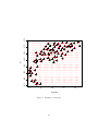
47.5
47.0
46.5
46.0
44.0
44.5
45.0
45.5
lat
6
8
10
longitude
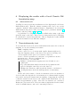
Figure 2: Example of Mapping
10
12
14
8
8.1
Examples
Example 1: 1-dimensional model with a barrier
In the Example directory of the archive LocalDiff.tar.gz we provide files to
run LocalDiff on a first simple example. The data were simulated using
the software ms ([3]). We assume that 30 populations evolved according to a
classical stepping-stone model. Five units of coalescent ago, a barrier to gene
flow arose between populations 15 and 16. Because of the barrier to gene flow,
we expect larger Local Genetic Differentiation measures for populations 15
and 16. The file Matrix1D.dat contains the matrix of pairwise correlations
of allele frequencies between the 30 populations, and the file Position1D.dat
contains the coordinates of those 30 populations.
A way to run LocalDiff here would be:
MyMachine $> ./LocalDiff -i Examples/Matrix1D.dat -p Examples/Position1D.dat
-o Examples/My1DResults -n 2 0.1 -s 200
To provide a LocalDiff map, run R
MyMachine $> R
and in the R command line, type
> source("Rfiles/Display1D.R").
8.2
Example 2: 2-dimensional model with a gradient of migrations
A stepping-stone model was also used for the second example. The species’
range is 2-dimensional species’ range with a grid (10×10) populations. There
is no barrier to gene flow here, but varying effective migration parameter,
which decreases from the south-west to the north-east. We expect Local
Genetic Differentiation to increase from the south-west to the north-east.
The file Matrix2DG.dat contains the matrix of pairwise correlations of allele frequencies between the 100 populations, and the file Position1DG.dat
contains the coordinates of those 100 populations.
The command line for running LocalDiff is
MyMachine $> ./LocalDiff -i Examples/Matrix2DG.dat -p Examples/Position2DG.dat
-o Examples/My2DResults -n 4 0.1 -s 200
To provide a LocalDiff map, run R
MyMachine $> R
and in the R command line, type
> source("Rfiles/Display2D.R").
11
8.3
Example 3: 2-dimensional model with 2 barriers to gene
flows
A stepping-stone model was also used for the second example. The species’
range is 2-dimensional species’ range with a grid (10 × 10) populations. 2
barriers to gene flow are present here, one between x = 5 and x = 6 at
T = 5. The other one between y = 7 and y = 6, x > 5, at T = 3. We
expect Local Genetic Differentiation to reveal those two barriers. The file
GenoBarrier2D.dat contains the matrix of genotypes of individuals from
100 populations, and the file Position1DG.dat contains the coordinates of
those 100 populations.
The command lien for running LocalDiff is
MyMachine $> ./LocalDiff -c Cor Examples/CorrelationMatrix HaploSNP
-i Examples/GenoBarrier2D.dat -p Examples/Position2DG.dat
-o Examples/My2DResults_2 -n 4 0.1 -s 200
To provide a LocalDiff map, run R
MyMachine $> R
and in the R command line, type
> source("Rfiles/Display2D_2.R").
8.4
More detailed plots
Raster file If you want to display the LocalDiff map on a specific region
only, you can use a raster file for that. An example of a raster file for displaying the locations above 1,000 meters is given. Generating a LocalDiff map
with this raster can be performed by sourcing the file DisplayFromascFile.R
in R.
Administrative Area If your species’ range corresponds to an administrative zone, country, county, city... you can use the global administration
areas data base to restrict the fircion map to the region of interest. How
to display the LocalDiff map for the human Swedish sample is shown in
DisplayFromgadmPolygon.R
References
[1] E. Anderson, Z. Bai, C. Bischof, S. Blackford, J. Demmel, J. Dongarra, J. Du Croz, A. Greenbaum, S. Hammarling, A. McKenney, and
D. Sorensen. LAPACK Users’ Guide. Society for Industrial and Applied
Mathematics, Philadelphia, PA, third edition, 1999.
12
[2] Blum M.G.B Duforet-Frebourg N. Non-stationary patterns of isolation
by distance: inferring measures of genetic friction. ArXiv, mois 2012.
[3] R.R. Hudson. Generating samples under a wright–fisher neutral model
of genetic variation. Bioinformatics, 18(2):337–338, 2002.
[4] Bruce S Weir and C Clark Cockerham. Estimating f-statistics for the
analysis of population structure. evolution, pages 1358–1370, 1984.
13